computation of complete synthetic seismograms for … · geophys. j. int. (1997) 130, 1-16...

Geophys. J. Int. (1997) 130, 1-16

Computation of complete synthetic seismograms for laterally heterogeneous models using the Direct Solution Method

Phil R. Cummins,' * Nozomu Takeuchi2 and Robert J. Geller2 ' Research School of Earth Sciences, Australian National University, Canberra ACT 0200, Australia Department of Earth and Planetary Physics, Faculty of Science, Tokyo University, Yayoi 2-1 1-16, Bunkyo-ku. Tokyo 113, Japan

Accepted 1997 January 17. Received 1997 January 17; in original form 1996 October 30

S U M M A R Y We use the Direct Solution Method (DSM) together with the modified operators derived by Geller & Takeuchi (1995) and Takeuchi, Geller & Cummins (1996) to compute complete synthetic seismograms and their partial derivatives for laterally heterogeneous models in spherical coordinates. The methods presented in this paper are well suited to conducting waveform inversion for 3-D Earth structure. No assumptions of weak perturbation are necessary, although such approximations greatly improve computational efficiency when their use is appropriate.

An example calculation is presented in which the toroidal wavefield is calculated for an axisymmetric model for which velocity is dependent on depth and latitude but not longitude. The wavefield calculated using the DSM agrees well with wavefronts calculated by tracing rays. To demonstrate that our algorithm is not limited to weak, aspherical perturbations to a spherically symmetric structure, we consider a model for which the latitude-dependent part of the velocity structure is very strong.

Key words: body waves, lateral heterogeneity, surfaces waves, synthetic seismograms.

1 INTRODUCTION

Several global and regional seismic networks using broad-band, high dynamic range, seismographs (Wielandt & Steim 1986) have now been established; high-quality digital seismograms from these networks are now widely available. Waveforms recorded by such instruments typically contain body waves, surface waves, and near-field effects in the frequency range from a few millihertz to several hertz. To exploit the infor- mation contained in such broad-band digital seismograms fully, waveform inversion (e.g. Tarantola 1984; Geller & Hara 1993) should be performed. Efficient and accurate methods for computing complete broad-band synthetic seismograms and their partial derivatives are thus required.

The purpose of this paper is to present methods for computing complete synthetic seismograms and their partial derivatives for laterally heterogeneous media with spherical coordinates. We compute synthetics using the Direct Solution Method (DSM) (Geller et of. 1990; Geller & Ohminato 1994), which is a method exploiting the Galerkin weak form of the elastodynamic equations. Hara, Tsuboi & Geller (1991, 1993)

*Now at: Japan Marine Science & Technology Center, 2-15 Natsushima-cho,Yokosuka 237, Japan.

used the DSM to compute surface-wave synthetics and their partial derivatives for a laterally heterogeneous earth model in spherical coordinates; they used the eigenfunctions of the degenerate singlets of the laterally homogeneous part of the model as the trial functions.

Cummins et al. (1994a,b) and Takeuchi, Geller & Cummins (1996) used the DSM to compute complete synthetic seismograms (i.e. synthetics including both body waves and surface waves with no far-field approximations) for laterally homogeneous media in spherical coordinates. Because separation of variables can be used for the laterally homogeneous problem, a relatively small system of banded linear equations is solved for each angular order f and azimuthal order m. In contrast, for the laterally heterogeneous problem all angular and azimuthal orders are coupled, so the computational requirements are much greater. Also, approximations such as truncating the coupling between different angular orders must in general be used. These points are covered in detail below.

This paper presents a complete frequency-domain formulation of a DSM algorithm for laterally heterogeneous models in spherical coordinates. The effects of anisotropy, self-gravitation and of the Earth's rotation are not included in this paper, but could be added in a straightforward way if desired. We present explicit results for the case in which the lateral variation of the elastic constants is expanded in terms

0 1997 RAS 1

2 P. R. Cummins, N. Tukeuchi and R. J. Geller

of spherical harmonics. The representation of the lateral heterogeneity in terms of some other parameterization can easily be achieved by replacing the sum over ‘J-squares’ intro- duced in Section 4 by some other form of coupling integral, such as the Legendre transformation method of Lognonne & Romanowicz (1990).

The contents of this paper are as follows. In Section 2, we summarize the key results for the DSM. In Section 3 we give the explicit form of the matrix elements and excitation for the laterally homogeneous case. Section 4 extends these results to the laterally heterogeneous case. Section 5 presents synthetic seismograms for some simple heterogeneous models. Section 6 compares our approach with those of other workers and discusses prospects for future research.

2 DIRECT SOLUTION METHOD

The Direct Solution Method (DSM) solves the Galerkin weak form of the elastic equation of motion to compute synthetic seismograms and their partial derivatives. General discussions of the weak form of PDEs from the standpoint of numerical computation are given by Strang & Fix (1973) and Johnson (1987). A more rigorous treatment is given in portions of several chapters of Dautray & Lions (1988). The DSM itself is presented in detail by Geller & Ohminato (1994); we summarize their results here without repeating the derivations.

2.1 DSM for fluid-solid media

We begin by considering a medium with both fluid and solid regions. Continuity of normal displacement and normal traction, and vanishing of the tangential traction, are required at all fluid-solid boundaries. Geller & Ohminato (1994) show that by adding appropriate surface integrals to the weak form of the equation of motion these continuity conditions become natural continuity conditions which are automatically satisfied by lhe DSM solutions.

The dependent variable in the solid regions is the displacement, which we expand in terms of vector trial functions, where w is the frequency, u, is the i-component of the displacement, @Ip’ is the i-component of the j t h trial function, cp is the expansion coefficient, and x is the spatial coordinate:

U j ( X , w ) = c c+8(w)@y’(X) f l ~ s o l i d

Note that throughout this paper we use @i to denote the components of the vector trial function in the solid portions of the medium, @ to denote the scalar trial functions in the fluid portions, and q5 to denote one of the spherical coordinates

Following Geller & Ohminato (1994), the dependent variable in the fluid regions is Q, which is linearly related to the pressure change, P. We expand Q in terms of scalar trial functions @)(XI:

( r , &4).

where 1 is the elastic modulus in the fluid, cp is the expansion coefficient of the Pth trial function, and ‘,k’ denotes differ- entiation with respect to the k-coordinate. Summation over repeated subscripts is implied when the subscripts refer to

a physical coordinate, but not when the subscript refers to an abstract vector space such as the vector space of trial functions.

The expansion coefficients of the trial functions, cp, become the unknowns in the DSM equation of motion. In general, we omit the arguments x and w in the remainder of the paper. We use a and P as the indices of the trial functions. Each of these indices is actually a pointer to a set of indices that characterize the trial functions. This is discussed in Appendix A of Geller & Ohminato (1994) and below.

One additional complication which was discussed by Geller & Ohminato (1994) should also be noted. If all or part of the outer boundary is a fluid region, we require Q = 0 at the outer boundary to satisfy the free-surface boundary condition. This is an essential boundary condition that must be explicitly satisfied by each of the scalar trial functions used in eq. (2 ) .

For a fluid-solid medium with a free-surface $oundary condition, and a solid region at the outer bounda y, the DSM equation of motion, eq. (46) of Geller & Ohmina / o (1994), is

(W*T-H+UR)C= - g , (3) where R is the matrix operator corresponding to the natural continuity conditions at the fluid-solid boundaries, T is the mass (kinetic energy) matrix, H is the stiffness (potential energy) matrix, and g is the vector of excitation coefficients. Eq. (3) will be singular whenever w is equal to an eigen- frequency. Since the elastic moduli throughout this paper include anelastic attenuation, all of the eigenfrequencies will be complex. Eq. (3) will therefore be non-singular for all real values of a.

The matrix elements and vector elements in eq. (3) are

[ 1, (@f’)*p@ip’ dV (a , 8) E solid

l o otherwise

(4)

(5)

otherwise

(@y))*n:’)@(p) dS CI E solid and fi E fluid

(@(a))*ny)@:P)dS a E fluid and E solid (6)

Rap = I l o otherwise

a E solid

(7) (@~~’)*J ; l (pw) d V a E fluid,

where * denotes complex conjugation, p is the density, CQkf is the elastic tensor in the solid, 1 is the elastic modulus in the fluid, and ny) is the outward unit normal to the solid regions at the fluid-solid boundaries. Anelastic attenuation is included in

Synthetic seismograms for laterally heterogeneous models using the DSM 3

cijkf and I , which are in general complex and frequency- dependent. Note that the subscripts on the left-hand side and the superscripts on the right-hand side of eqs (4) to (7) refer to the abstract vector space of trial functions; the subscripts on the right-hand side of these equations refer to the physical space.

@ f j in the first line of eq. (5 ) denotes the locally Cartesian derivatives. The locally Cartesian derivatives of a vector ur in spherical coordinates are given by:

Similarly, the locally Cartesian gradient of a scalar A (see the second line of eq. 5 ) for spherical coordinates is given by

(9)

2.2 Partial derivatives of synthetics

The Galerkin form of the first-order Born approximation is

(02T - H + OR) 6c = -to2 (ST) - ( ~ H ) ] c , (10)

where the matrices on the right-hand side of eq. (10) correspond to infinitesimal perturbations to the elastic moduli and density. Eq. (10) could be extended to include terms from eq. (6) if the location of a fluid-solid boundary is perturbed, but we do not present explicit results here.

To perform iterative linearized inversion for Earth structure, it is not necessary to solve eq. (10) once for each earthquake and each model parameter. Rather, we formally write the solution of eq. (10) as

6~ = - (O~T-H+OR)-' [ W * ( ~ T ) - ( ~ H ) ] c , (1 1) and then, as discussed by Geller & Hara (1993), incorporate eq. (11) into the expressions for the coefficients of the normal equations for the waveform inversion problem. The end result is that we have to solve eq. (3) once for each source and a similar equation once for each component of the displacement at each receiver. The latter equation gives the 'back- propagated' wavefields, and the partials are then found by evaluating a bilinear form. As discussed below and in Geller & Hara (1993), this can form the basis of a highly efficient waveform inversion algorithm.

3 LATERALLY HOMOGENEOUS MODEL

The results in the previous section are completely general. In this section we present the explicit form of the matrix elements for a laterally homogeneous model. These results have already been presented by Cummins el al. (1994a,b) and Takeuchi etal.

(1996), but we summarize them here as they are required for the discussion of the laterally heterogeneous problem in the next section. We henceforth restrict the discussion to an isotropic medium, for which the elastic tensor in the solid region is

Ctlkl =A&$kl+ P(hik6j1+ d r d j k ) , (12)

where 3, and p follow the standard definitions, and a,, is a Kronecker-6. Note, however, that the methods of this paper can be extended to the anisotropic case in a straightforward fashion if desired.

3.1 Trial functions

The trial functions defined below are also used in the next section for the case of a laterally heterogeneous model. We denote the trial functions in the solid as and a!'), where u-+{k'e'm'p'} and fl-{kemp} are respectively pointers to k and k , the indices for the linear splines, l' and e , the angular orders, m' and m, the azimuthal orders, andp' abd p , the indices for the polarization of the trial functions.

We use three types of vector trial functions, @(kPmp),

p=1,2,3, in the solid regions of the medium. The depth- dependent part of all three types of vector trial functions is given by linear splines, and the horizontal dependence is given by the three fully normalized vector spherical harmonics, as shown below. The first two types of trial function, @(kEm')

and @(ke'n2), have spheroidal polarization, and the third type, @(kBn'3), has toroidal polarization. We first define fully normalized vector spherical harmonics as follows:

where the Ypm are fully normalized surface spherical harmonics and L= d m . The explicit form of the vector trial functions is

The arguments ( r , Q , $ ) will in general be omitted in the remainder of this paper.

The scalar trial functions in the fluid regions are

We denote the trial functions in the fluid as @('I and where a-~{k'elm'} and fl-+{ki?m} are respectively pointers to k and k , the indices for the linear splines, t' and .t the angular orders, and m' and m the azimuthal orders. There are four indices for the solid case, but only three for the fluid case, because we have an additional index, p' or p , for the polarization of the trial functions for the former.

It is implicit in eqs (4) and (5) that a separate set of trial functions is being used for each fluid region and each solid region, and that the coupling between the solid and fluid regions is entirely accounted for by the matrix elements in

0 1997 RAS, GJf 130,l-16

4 P. R. Cummins, N. Tnkeuchi and R. .I. Geller

eq. (6). In the present paper we use one set of trial functions for the inner core, a second for the outer core, and a third for the mantle and crust; each of these regions is allowed to be arbitrarily heterogeneous in the vertical direction. For each set of trial functions we define a separate set of linear splines of the following form to specify the depth dependence of the trial functions:

( r - q - I ) / ( r k - r k - 1 ) r k - 1 < r<rk

&Ad= ( r k + l - r ) / ( r k + i - r k ) r k s r < ~ + l (16) i 0 otherwise.

We thus have one set of splines for the inner core, a second for the outer core, and a third for the mantle and crust. The first line of eq. (16) is ignored for the lowermost layer of each region, and the second line of eq. (16) is ignored for the uppermost layer of each region.

Each of the trial functions must satisfy certain essential continuity conditions: continuity of displacement in the solid regions, and continuity of Q in the fluid regions. The trial functions defined in eqs (13) and (15) satisfy these essential continuity conditions when the splines are defined using eq. (16). Since continuity of traction (in the solid), and continuity of the i-component of the displacement in the i-direction (in the fluid) are natural continuity conditions, the nodes of the spline functions in eq. (16) can in principle be chosen without regard to the location of first-order discontinuities in the elastic constants. However, the greatest accuracy can be achieved by ensuring that each first-order discontinuity is a node for the spline functions (otherwise the traction in the solid or the displacement in the fluid will, in effect, be constrained to be discontinuous).

3.2 Matrix elements

Due to the following selection rules for matrix elements (e.g. Phinney & Burridge 1973; Jones 1985) for a laterally homo-

(a) Spherically Symmetric Case

0-1

geneous, isotropic, medium, only a few of the matrix elements in eqs (4), ( 5 ) , and (6) will be non-zero, and due to degeneracy many of these will be equal. In particular:

(1) All of the matrix elements will be zero unless !=Y and rn = rn'.

(2) All of the matrix elements for coupling between the toroidal (p= 3) and spheroidal (p= 1 or p = 2 ) trial functions are zero.

(3) Because of the degeneracy of the spherically symmetric model, the matrix elements depend only on e, and are independent of rn.

(4) Because, as shown by eq. (16), the kth spline is only non- zero in the interval r k - 1 < r < r k + 1, all of the matrix elements in eqs (4) and (5) will be zero unless Jk-k'ls 1.

As a consequence of the above selection rules, we can decompose eq. (3) into separate systems of linear equafons for each e and rn; we can further divide these systems into separate systems for spheroidal (p = 1 or p = 2) and toroidd (p = 3) displacement (see Fig. la). Although, as noted above, the matrix of coefficients on the left-hand side of eq. (3) depends only on e, the excitation coefficients on the right-hand side of these equations will depend on both l and rn. If the source is a point force on the z-axis, the right-hand side will be non-zero only for (rn( I 1; if the source is a point moment tensor on the z-axis, the right-hand side will be non-zero only for Irnls2.

The integrals over dS can be analytically evaluated to reduce the expressions for the matrix elements in eqs (4), (5), and (6) to expressions which depend only on the depth, r . Because the ath and j t h trial functions have the same angular and azimuthal orders, we omit the angular and azimuthal order numbers in the following discussion. We thus, for example, write the matrix element T.p for a solid as Tppz,kp (rather than Tpcmy,ktmp); i.e., we show only the indices for the spline function and polarization of the two trial functions explicitly. In the following equations we write the derivative with respect to the depth of the kth trial function, d&/dr, as X k .

I

(b) Toroidal Axisymrnetric Case

CMB - r- Surfa

Surface

3

Figure 1. The structure of the DSM matrix. Grey shading indicates the location of non-zero elements; where there is no grey shading, the elements are zero. For simplicity, no fluid layers are included, although the structure is similar for mixed fluidisolid media. (a) Both spheroidal and toroidal matrix elements for the spherically symmetric case. (b) The toroidal matrix elements only, for the azimuthally axisymmetric case.

0 1997 RAS, GJl 130,l-16


We begin by considering the explicit form of eqs (4) and (5 ) for a solid region, i.e. (a, /I) E solid. [In our own work we use the linear splines given by eq. (16), but the following expressions could also be used for other choices of the vertically dependent part of the trial functions.] We begin by defining the following intermediate integrals involving the splines. The upper and lower limits of integration are not shown explicitly, but can be readily determined from the nature of the splines being used:

= drpr2&& , J = dr ixkxk ,

I ; ,~ = drh.&xk ,

Note that xk is differentiated in Iirk while is differentiated in

Using the above intermediate expressions, the matrix I;>k.

elements are

Tkp,,kp = { if ' = ' I

otherwise,

forp=l andp'=2

forp=2andp'=l

(L2 - l)I;,k - I;,k - I;v + I;,k for p=p'= 3

I 0 otherwise.

(19)

Note that some of the subscripts for I 2 and I s in eq. (19) are kk , rather than kk .

The linear spline trial functions defined in eq. (16) can be substituted into the above operators to obtain matrix elements for eq. (3). Finer grids will lead to more accurate solutions. However, by using modified operators whose explicit form is given by Geller & Takeuchi (1995) and Takeuchi et al. (1996) the same accuracy can be achieved using a much coarser grid (and hence much less computation time).

The operators in eqs (18) and (19) are dominated by the terms proportional to L210, L211, L214, LIZ, LI', 13, and 16. We replace the first five of these terms by the modified operators. Other terms (e.g. the second term in the first line of eq. 19) are not replaced by modified operators. Note that the modified operators for I' and 1' are in some cases non-zero for Ik-k'l= 2, but the bandwidth of the matrices does not increase, due to the arrangement of the matrix elements (see Geller & Takeuchi 1995 and Takeuchi et a/. 1996).

We next present similar results for the matrix elements for a fluid region. We first define the following intermediate integrals:

As discussed by Takeuchi et a/. (1996), we use modified operators in place of I , : and I;;.

Using the above intermediate expressions, the matrix elements for a fluid are

Finally, we consider the explicit form of the matrix element at a fluid-solid boundary (see eq. 6) for the a(-+{k'e'm'})th trial function in the fluid region and the /I( -{k!mp})th trial function in the solid. ny' is the component of the outward normal vector to the solid in the (1,0,0) direction, n!j' is the component of the normal vector in the (0, aY/m/ae , ( l / s inB)a~~ /a# ) /L direction, and ny' is the component of the normal vector in the (O,(I/sinf?)aY~ml~#, -aY/,,,/aO)/L direction. Since in this section the medium is laterally homogeneous, the normal vector is always in the vertical direction, and eq. (6) reduces to

where all of the quantities in eq. (23) are evaluated at the depth of the fluid-solid boundary. If there is more than one fluid- solid boundary, the matrix R in eq. (3) is the sum of the terms for each interface from eq. (23). Since the unit normal vector points outward from the solid, n';" = - 1 at the core-mantle boundary (CMB), and ny' = 1 at the inner-core boundary (ICB).

3.3 Excitation

In discussing the excitation it is useful to introduce the com- monly used functions UF(r), VT(r), and W?(r), which give the depth dependence of the spherical harmonic components of the displacement:

~ ( r , 0, $1 = C ~ , " ( r ) s ; ~ ( e , 4) + v,"(r)s;m(e, 4) Im

+ w n ) T e m ( & 4). (24)

In terms of the trial functions used in this paper we can express U,", VT, and Wj" as follows:

0 1997 RAS, GJI 130,1-16

6 P. R. Cummins. N. TukeuchiundR. J. Geller

Even if the modified operators are used, the expansion coefficients still give the value of UpM, V r , and W r at the nodes:

u?(rk)=ck!ml 3

WTo‘k) = cktm3 .

In this section we drop the subscripts e and rn on U , V , and W , as we are considering the laterally homogeneous case. The excitation is obtained from eq. (7). We consider the case of a point moment tensor on the z-axis (r = rs, I$ = 0, &O), in which case the right-hand side of eq. (7) is zero except for IrnlS 2. The excitation vector g can be determined by straightforward application of eq. (7). However, the body-force equivalents for certain moment tensor terms are kinematically equivalent to requiring U(r),V(r), or W ( r ) to be discontinuous at the source depth (e.g. Takeuchi & Saito 1972, p. 290). This is an essential boundary condition that will be violated by a straightforward application of eq. (7), thereby leading to suboptimal convergence (Strang & Fix 1973).

It is preferable to incorporate the displacement discontinuities directly into the definitions of U(r) , V(r) , and W(r) (see Cummins et al. 1994a,b). The discontinuities are given by Takeuchi & Saito (1972, p. 289):

DI = U(r)l$ =bi6mo2Mrr/[r;(A,~f2/*,)lj

02 = V ( Y ) I $ = hl an,+ 1 (T ~ , o + ~ M , $ ) I [ ~ ; P J , (27)

D3= W(r)I$ =blL+i(iMro k M r $ ) / [ r : ~ ( r s ) l ,

where As=A(rs) , ps=/*(r .J , and b1=[(2!+1)/167~]”~. The remaining source terms involve discontinuities in the

radial traction at the source depth, which is a natural boundary condition. Once the essential boundary conditions eqs (27) are incorporated into the definitions of U , V , and W , the remaining, source terms are taken into account via straightforward application of eq. (7) to obtain:

gkl = b ~ 6m02[M@8 i- M44 - Mrr2&/ (As + 2P,JIXk(rs)/rs,

g k ~ = b i 6 ~ d - M o e -Mq$ +Mrr2&/(& +2&)I&(rS)/rr

- bzfi, + z(M46 - Moo k i2Mom)&(r,) 1 r, ,

gk3 =b2fim+2(f ~ M R H f iM64 -2Mo,,+)Xk(rJ/r,,

where b2 =[(2!+ l)(!- l ) ( l + 2 ) / ( 6 4 ~ ) ~ / ~ ] and bl is defined above.

The above formulation is sufficient for sources located at nodes, but it is desirable to be able to compute synthetics for arbitrary source depths. This can be done either by representing the solution in the source layer as the sum of a general solution of the form of eq. (1) and a particular solution, or by using a ‘source box’ formulation. A detailed discussion of the necessary results will be presented in a separate manuscript.

(28)

3.4 Numerical and computational considerations

As discussed above, for the laterally homogeneous case we decompose eq. (3) into separate systems for each angular order e and azimuthal order rn. We then further decompose these systems into one set of linear equations for the toroidal

displacement and one for the spheroidal displacement. The coefficients in the matrix on the left-hand side of each of these systems of linear equations depend only on C and not on rn. Each of the coefficient matrices is banded; the bandwidth (including the diagonal) is 3 for the toroidal and fluid cases, and 7 for the spheroidal case in the solid (see Fig. la).

We use Cholesky decomposition, followed by forward- and back-substitution, to solve the systems of linear equations. The former operation requires O(Nx N t /2) floating-point operations (FLOPS), while the latter requires only O(4NxNb) FLOPS, where Nb is the bandwidth. However, the former operation need be performed only once for each angular order e, while the latter is required once for each right-hand side. This is a crucial point when dealing with a large number of sources and/or partial derivatives, as it means that the increpental computation time required for each additional source or partial derivative is minimized.

4 LATERALLY HETEROGENEOUS MODEL

In this section we derive the explicit form of the matrix elements for a laterally heterogeneous model. We restrict the discussion to an isotropic model, but these results can be extended to the anisotropic case in a straightforward fashion, using the results of Jones (1985, p. 164-166) or Mochizuki (1986). Su, Park & Yu (1996) and Yu & Park (1996) also discuss the inclusion of anisotropy in normal-mode calculations.

For the isotropic case, the elastic moduli A and p, and density p , at any radius r can be expressed as a sum over spherical harmonics:

F f

f = O g = - f

F f

F f

In general F = co, but it is necessary to use a finite F in actual calculations. The expansion coefficients in eq. (29) depend on r , but we omit this dependence below, writing simply L!, $, and p:.

4.1 harmonic indices

For the laterally homogeneous case, the choice of trial functions eq. (13) results in surface integrals for the matrix elements that are easy to calculate: they are zero when C # e or m’#rn, and can be evaluated analytically when C=C and rn‘=m. In contrast, for the case of a laterally heterogeneous model with elastic properties of the form (29), the matrix elements are in general non-zero whenever le‘-ll<F and m‘ = m + g , and zero for all other cases. In this sense we can say that within a bandwidth + F about the diagonal defined by e‘ = e , m‘ = rn, trial functions having spherical harmonic indices t‘, rn’ are coupled to trial functions having indices e , in.

The surface integrals that are non-zero can be analytically expressed in terms of Wigner 3-5 symbols (see, e.g., Edmonds

Trial functions and coupling of spherical

0 1997 RAS, GJI 130, 1-16

Synthetic seismograms for laterally heterogeneous models using the DSM I

~ f e ' z f , k [ p , .] i f p = l '

Ifrk [ i, 0 1 1 i fp=2 ,3

min(F,e' +o Tke'm'p,klmp=

f= Ie' -PI e . f e

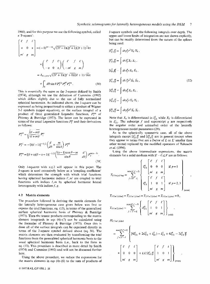
1960), and for this purpose we use the following symbol, called a 'J-square':

>

I;, ; =(-1)(" '-" 'J (2C+ 1)(2f + 1)(2!+ 1)/4.n

This is essentially the same as the J-square defined by Smith (1974), although we use the definition of Cummins (1992) which differs slightly due to the use of fully normalized spherical harmonics. As indicated above, the J-square can be expressed as being proportional to either a product of Wigner 3-5 symbols (upper equation), or the surface integral of a product of three generalized Legendre functions, Py of Phinney & Burridge (1973). The latter can be expressed in terms of the usual Legendre functions PT and their derivatives as follows:

(a-l)cos%-m d sin 8 fy = [(l+ a,(e- c! + 1)]-

Only J-squares with a 1 2 will appear in this paper. The J-square is used extensively below as a 'coupling coefficient' which determines the strength with which trial functions having spherical harmonic indices P, m' are coupled to trial functions with indices !, m by spherical harmonic lateral heterogeneity with indices f, g .

4.2 Matrix elements

The procedure followed in deriving the matrix elements for the laterally heterogeneous case given below was first to express the trial functions, eq. (13), in terms of the generalized surface spherical harmonic basis of Phinney & Burridge (1973). Then the tensor products corresponding to the matrix element integrands in eqs (4)-(7) can be calculated using the formulae of Phinney & Burridge (1973). Once this is done all of the surface integrals can be expressed directly in terms of the J-square symbol defined above (eq. 30). The matrix elements are then evaluated by transforming the trial functions from the generalized spherical harmonic basis to the usual spherical harmonic basis (i.e., back to the form in eq. (13). This procedure is described in more detail by Smith (1974) and Cummins (1992) and will not be discussed further here.

Using the above procedure, we reduce the expressions for the matrix elements in eqs (4)-(6) to the sum of products of

J-square symbols and the following integrals over depth. The upper and lower limits of integration are not shown explicitly, but can be readily determined from the nature of the splines being used:

0 1997 RAS, GJI 130,l-16

Note that Xk is differentiated in while Xk, is differentiated in Z& The subscript f and superscript g are respectively the angular order and azimuthal order of the laterally heterogeneous model parameters (29).

As in the spherically symmetric case, all of the above integrals except [Z:,,$ and [Z&J? are in general (except when they appear in terms that are a factor of L or L smaller than other terms) replaced by the modified operators of Takeuchi et al. (1996).

Using the above intermediate expressions, the matrix elements for a solid medium with lP -i? 2 F are as follows:

I r p f l l

8 P. R. Cummins, N. TakeuchiandR. J. Geller

P f !

0 0 0 1

m' g m

where Q;= J(l' + 2)(P - 1) and Q2 = J(! + 2)(! - 1). The remaining elements can be determined from the following symmetries of the T and H matrices:

Trem,kem2= - Tkrm'2,kem3 ,

Hk'e'm'3,k!m2= -Hk'Y'm'2,ktm3 ,

Hke.mr2,kem1 = H k t n i l , k ~ m 2 ,

Hk'e'm'3,kPmi = -Hkt'm'l,k!m3 3

(34)

For ll'-!l > F, all of the matrix elements are zero. The (even), (odd) subscripts indicate that, in the sum over f , only the terms with l' + ! + f even or odd, respectively, are included. Note that the (even) terms correspond to spheroidal- spheroidal or toroidal-toroidal coupling, while the (odd) terms correspond to spheroidal-toroidal and toroidal-spheroidal coupling.

As can be seen from eqs (4)-(6), the matrices T and H for the elastic case (i.e., cek/ real) are Hermitian, for example Tprm'p',kgmp = T * k ~ , ~ , p ~ ' ~ i ~ , . For the spherically and axially symmetric cases, the coupling coefficients are all real and T and H are real symmetric for the elastic case and complex symmetric for the anelastic (i.e., c ! j k { complex) case, for example Tk,pmy,kPmp = Tkpmp,pTm'p'. However, for the general 3-D, anelastic case the matrices T and H are complex but neither symmetric nor Hermitian. The matrice T and H can be made complex but symmetric by performi d g a transformation of the complex spherical harmonic basis into one which is real, but we will not present explicit results for this here.

We next derive similar results for the matrix elements for a laterally heterogeneous fluid region. We begin by defining the following depth integrals as intermediate quantities:

Using the above intermediate expressions, the matrix elements for a fluid are

The first two integrals in eq. (35) are replaced by modified operators in our calculations.

In the results presented in this paper all of the boundaries are spherically symmetric, and explicit expressions for the elements of the matrix R of eq. (6) for this case are given by eq. (23) of the previous section. If the boundaries were also laterally heterogeneous, this would have to be taken into account in calculating the elements of R, as well as those elements of T and H which involve trial functions defined on the boundary. In general, these matrix elements will involve surface integrals for which there is no exact analytical expression. However, if the topography is small it is possible

0 1997 RAS, GJZ 130, 1-16


to derive analytical expressions for the matrix elements which are accurate to first order in the deviation of the boundary topography from a spherical surface. Again, explicit results will not be presented here.

4.3 Implementation

The ordering of the trial functions is chosen to optimize computational efficiency. Generally speaking, this is achieved by an arrangement which concentrates the non-zero matrix elements as closely as possible to the diagonal (see Appendix A of Geller & Ohminato 1994). In the spherically symmetric case considered above and by Cummins et al. (1994a,b) and Takeuchi et al. (1996), there is no coupling among elements having different angular orders or azimuthal orders, so that elements in a row corresponding to angular order 1 and azimuthal order m and a column corresponding to angular order c' and azimuthal order m' are zero if !#!' or m#m'. Furthermore, the matrix elements for coupling between spheroidal (p = 1,2) and toroidal (p = 3) trial functions are zero. In this case the obvious way to organize the coefficient matrix in eq. (3) is to order the trial functions so that the equation of motion is divided into separate blocks for each angular order, and then to divide these in turn into separate blocks for each azimuthal order. Owing to the degeneracy of the laterally homogeneous problem the matrix elements are independent of azimuthal order, but the excitation coefficients and expansion coefficients depend on both @ and m. The blocks for each given 1 and m are then further separated into spheroidal and toroidal blocks. Within each block the index corresponding to the polarity p varies most rapidly, with the index for the radial grid point k varying less rapidly. Note that the variation over p is trivial for the toroidal case (for which p=3), but non-trivial for the spheroidal case, for which we have trial functions with both p = 1 and p = 2. The result of this ordering is a block diagonal matrix with each block along the diagonal having very narrow bandwidth. As the various blocks are completely decoupled, each block can be decomposed individually (see Fig. la, where the grey areas denote non-zero matrix elements).

In contrast, for the case of laterally heterogeneous structure, all angular and azimuthal orders, and polarities, are in general coupled. There are some special laterally heterogeneous cases where there is partial, but not full, coupling between different angular and azimuthal orders and polarities. We consider a model with axisymmetric (i.e. g=O) lateral heterogeneity. In this case the matrix elements with row and column indices corresponding to different azimuthal orders will be zero, i s . there is no coupling between different azimuthal orders. For this case the DSM matrix A is symmetric, even for the anelastic case. As our goal is to concentrate the non-zero matrix elements close to the diagonal, we use the alternative arrangement of matrix elements shown in Fig. l(b) for this case. In this arrangement the index corresponding to the polarization p varies most rapidly, followed by the index for the angular order !, followed by the index corresponding to the radial grid point k.

In general there will be toroidal-spheroidal coupling even for an axisymmetric (g=O) model, but there is no toroidal- spheroidal coupling for the case m=m'=O. To see this, note that one of the symmetry conditions for the coupling

coefficients is

L-mr -g - m J

When m' = g = m = 0, the above reduces to

(37)

However, for toroidal-spheroidal coupling one of the selection rules is t'+!+f=odd, we therefore obtain from eq. (38) for this case

c ' f e

0 $0. / I

(39)

Thus as long as we restrict ourselves to a source that excites only m=O waves (e.g. a ring-source on the z-axis), there will be no toroidal-spheroidal coupling. Note that this is not a physically realizable source, as it imparts a net torque to the Earth. It is chosen purely to simplify the calculations presented here by allowing us to neglect toroidal-spheroidal coupling.

In the toroidal case the polarization index has only one value (p=3). The coefficient matrix for our problem again has a block structure, but now the dimension of each block is L a x X L a x , where !=O, ..., L,,,. The index corresponding to the radial grid point k now varies least rapidly, so the submatrices corresponding to the CMB are in the upper-left corner, and progress to those corresponding to the Earth's surface in the lower-right corner.

The value of L,,, will be finite, and can be determined using the selection rules, if the value of F , the maximum angular order of the lateral heterogeneity, is finite. On the other hand, for the real Earth F will in general be infinite. In this case the laterally heterogeneous model must be arbitrarily truncated at some maximum value, and truncation of the coefficient matrix in the equation of motion will usually also be necessary. The trade-offs between accuracy and computational requirements involved in such truncation remain an important topic for future study.

Cholesky decomposition proceeds in column-wise fashion from left to right, and for a matrix having the structure illustrated in Fig. l(b) it can be performed blockwise. To illustrate this we consider the simple case in which there are only two radial grid points, at the CMB and the Earth's surface. The Cholesky decomposition of the whole DSM matrix A = w2T - H appears as:

A=UTU,

where U is an upper triangular matrix. Expressed in block form, this becomes

where UOO, U ~ I , and Uol are the upper left, lower right, and off- diagonal submatrices of U, the upper triangular Cholesky decomposition of the DSM matrix A. Performing the

0 1997 RAS, GJI 130,l-16


above matrix multiplications results in the following matrix equations for Uoo, U11, and Uol:

Aoo = u&uoo >

The matrix products on the right-hand side of (42) have the form of Cholesky decompositions, and the way to carry out the block decomposition of the matrix illustrated in Fig. l(b) is clear: the upper-left submatrix is Cholesky decomposed to obtain UOO, then this is back-substituted onto the columns of Aol to obtain Uol, and then the result of subtracting U&Uol from All is Cholesky decomposed to obtain U I I . This procedure can be continued through all of the block submatrices illustrated in Fig. l(b) from the CMB to the surface to obtain the full Cholesky decomposition of A.

This block decomposition procedure has important con- sequences for the computational efficiency of the algorithm. First, the only part of U needed to obtain the Cholesky decomposition of a given submatrix along the diagonal is the off-diagonal submatrix immediately above it, i.e. to obtain U11 in (42) we only require Uol. Thus, as we proceed from upper left to lower right through the DSM matrix A, we do not need to store more than two submatrices of the original or decomposed matrix at one time (Cholesky decomposition can be performed in place, so no additional storage is required). Also, as the decomposition proceeds through the radial grid point corresponding to the source depth, the back-substitution can be performed on the source so that even the submatrix decompositions above the source depth can be discarded after use. If seismograms are required only at the surface, we only need to store two submatrices. If seismograms are required below the surface, we need to store two submatrices for each radial grid point between the surface and the receiver depth. In either case, ihe fact that we only need to access two submatrices at any one time leads to a tremendous reduction in memory requirements.

If the earth model is taken to be laterally homogeneous below some depth, say for the inner and outer core, the submatrices in Fig. l(b) corresponding to these depths are all diagonal. In this case the submatrix decompositions are trivial and can again be performed in place, leading to a great reduction in computation time. Finally, note that when the laterally heterogeneous structure is weak and band-limited (i.e., with lateral heterogeneity only up to some finite maximum angular order), it may be useful to neglect coupling between widely separated angular orders. In this case all of the submatrices in Fig. l(b), as well as the corresponding matrix decompositions, are banded, and standard sparse matrix techniques can be used for their storage and manipulation.

5 EXAMPLE COMPUTATION

The accuracy of the numerical solutions for the laterally homogeneous case was considered by Cummins et al. (1994a) and Takeuchi et al. (1996). Two questions are involved in such testing. The first is to make sure there are no bugs. To verify this the above papers compared the DSM solution for a given angular order to an independent numerical solution computed using the strong form of the equation of motion. They found that if extremely fine meshes were used for both methods the

numerical solutions could be made to agree to seven or more significant digits, thereby confirming the accuracy of both methods as well as the software.

A second question is the accuracy achieved by the DSM calculation for a given mesh size. Geller & Takeuchi (1995) showed that for a homogeneous medium the relative error of synthetics computed using the modified operators was

(43) 3.3

(elements/vertical wavelength)2 ’ relative error zz

If the grid spacing for a laterally homogeneous problem in spherical coordinates is chosen to have a roughly constant number of elements per vertical wavelength, eq. (43) can be used to make rough estimates of the accuracy of the DSM synthetics for a spherically symmetric model.

The above questions are more difficult to &ess for a laterally heterogeneous model. The standard problem most often used to validate methods for computing synthetic seismograms in laterally heterogeneous media is the calculation of Aki & Larner (1970) for plane SH waves incident on a 2-D basin. This problem, however, is in Cartesian geometry and thus cannot be used to test our algorithm for global- scale problems involving long-period (usually>lO s) waves. Standards of comparison for the latter problem are only now being developed (e.g. Igel et al. 1995). In our numerical examples we therefore present comparisons of our synthetics to wavefronts obtained using the ray-tracing method of Sambridge & Kennett (1990). Error estimates remain a topic for future work.

We present a simple numerical example. The model, the source, and therefore the wavefield are all azimuthally axisymmetric, so as discussed above there is no coupling between the toroidal and spheroidal wavefields, or between different azimuthal orders. The model (Fig. 2) consists of an azimuthally symmetric perturbation to the upper-mantle (i.e. above 660 km depth) shear velocity of a spherically symmetric model consisting of the shear-velocity profile of IASP91 (Kennett & Engdahl 1991) and the density and Q profile of PREM (Dziewonski & Anderson 1981). The azimuthally symmetric shear-velocity perturbation has maximum angular order F = 6, and increases smoothly from zero at 0 = 0 to a 110 per cent increase in shear velocity (as measured at the base of the upper mantle) at Q=n/2 , and then decreases smoothly again to zero at B = n. The lateral heterogeneity of the above model is unrealistically strong, for two reasons: (1) so that the differences between the wavefields for the 3-D and the spherically symmetric model would be obvious, and (2) to demonstrate that neither the theory nor the implementation of the DSM for a laterally heterogeneous model is restricted by ‘weak perturbation’ assumptions. The source is an azimuthally symmetric ring source, i.e. an m=O point source in the 4 direction, at a depth of 600 km at 0 = 0.

The wavefields are presented in Fig. 3. Wavefield calculations at the corresponding times are also presented for the spherically symmetric model. The 4 component of displacement is represented as a grey-scale, with white pointing into the plane of the figure and black pointing upwards. The weak bands of alternating dark and light ‘ripple’ are caused by the acausal filtering. The black curves are wavefronts obtained by ray tracing for the same model. The wavefronts obtained using ray tracing are usually advanced somewhat from the centre

1 .

0 1997 RAS, GJI 130, 1--16


Figure 2. The velocity model used in the wavefield calculations shown in Figs 3(a), (c), (e) and (8). This is basically IASP91 with a very strong azimuthally axisymmetric (g=O,f<6) shear-velocity perturbation in the upper mantle ( r > 571 1 km). Superposed are rays traced in the laterally heterogeneous model (solid curves) and the unperturbed IASP91 model (dashed curve), which illustrate the effect the model perturbation has on the ray paths. The end points of all three rays correspond to the time of the snapshots in Figs 3(g)-(h) (T= 1648 s). Note that the figure is rotated 90" so that the north pole (f l=O) is at the left, and the south pole (fl=n) is at the right.

of the white bands, due to the physical dispersion associated with the Q model used to compute the synthetics. The calculations were performed for 128 frequencies from 0.24 to 31.25 mHz, and cosine tapers were applied to the spectra in the ranges 0.0-0.5 mHz and 20-31.25 mHz. Angular orders were summed to a maximum of e = 350. 24 hours on a DEC Alpha 2000 workstation were required to produce the wavefield throughout the entire mantle. Note that the computation time would have been much shorter if only the seismograms at the Earth's surface were required.

At T=400 s the wavefield in Fig. 3(a) has propagated through a region in which the lateral heterogeneity is very weak, so it is virtually identical to that of the laterally homogeneous model (Fig. 3b). Direct S and sS are most prominent. ScS is also visible near the CMB, as are some weak reflections from the upper-mantle discontinuities. At T = 1008 s (Figs 3c and 3d), interaction with the surface and CMB has produced a number of additional phases such as SS and sScS. The effect of the lateral heterogeneity on the S wave in Fig. 3(c) is appreciable, as it has moved much more rapidly through the upper mantle than the S wave in Fig. 3(d). The strong velocity contrast at r = 571 1 km, 0 z 70" in Fig. 3(c) results in a pro- nounced kink in the S wavefront there, as well as a strong underside reflection (S660S in Fig. 3c), where the direct S wave is incident on the 660 km discontinuity from below. The latter phase is not evident in Fig. 3(f), because the velocity contrast at the 660 km discontinuity is very weak and does not vary with 0.

The Y-shaped features in the SS wavefronts in Figs 3(c)-(d) occur where these wavefronts fold back on themselves due to interaction with the positive velocity gradients in the mantle. They occur where the wavefronts touch the caustic surface associated with the corresponding system of rays. A similar

feature develops in the SSS wavefronts in Figs 3(e)-(h). A major difference between the wavefields for the laterally heterogeneous model (Figs 3a, c, e and g) and those for the spherically symmetric model (Figs 3b, d, f and h) is that the caustic surfaces tend to penetrate much more deeply into the mantle for the former.

Figs 3(e)-(f) are snapshots at T = 1296 s. Many more phases are now visible, including sSS, SSS, and sSCSS, which are labelled in the figures. The wavefield for the laterally heterogeneous model (Fig. 3e) differs greatly from the spherically symmetric case (Fig. 3f ) . Phases propagating in the upper mantle near 8 = n / 2 in Fig. 3(e) are far advanced compared to the corresponding phases in Fig. 3(f), and several of the ray- traced wavefronts are broken up after encountering the strong velocity contrast at r = 571 1 km near 0 = n/2. This is especially noticeable for sS and SS, whose up-going rays are post- critically reflected back into the lower mantle near r = 571 1, 0z70°. Note also the sharp kink in the ScSS wavefront near r=4500 km and 0 z n i 4 in Fig. 3(e). This phase travels twice through the upper mantle at a high angle of incidence, so its wavefront is diagnostic of structure there; in this case the kink reflects the transition with increasing 0 from low to high velocity in the laterally heterogeneous model.

At T=1648 s in Fig. 3(g) we see that the wavefield 'truncated' by the shear-modulus perturbation in the upper mantle, compared to that in Fig. 3(h), because there are essentially no geometrical arrivals there except for the small segments of wavefront appearing near the surface at Oz37ti4. Energy which was not able to penetrate the high-velocity 'cap' in the upper mantle near 0=7c/2 continues to bounce around in the lower mantle. Although and SSdiff in Figs 3(g)-(h) are barely visible at this scale, careful inspection shows them to be present in both figures (at the positions indicated) with

0 1997 RAS, GJI 130,l-16

12 P. R. Cummins, N . Takeuchi and R. J. Geller

(a) T=400s Laterally heterogeneous model

Figure 3 . Snapshots of wavefields 400 s after the origin time for (a) the laterally heterogeneous model illustrated in Fig. 2, and (b) the IASP91 model. The annular region represents a slice of the mantle, with the inner boundary of the annulus being the CMB and the outer boundary the earth's surface. The ring source which generated the waves was at r = 5771 km near the lower right boundary of the diagram. Source, model, and wavefield are all azimuthally symmetric (m=O). The dark curves superposed on the wavefield are wavefronts interpolated from the results of tracing rays through the same model as was used in the wavefield calculations (except that the model for the former was elastic whereas the model for the latter included anelastic attenuation and hence physical dispersion). Note that the figures are rotated 90" so that the north pole (0 = 0) is at the left, and the south pole ( 0 = n ) is at the right. (c) and (d) are as (a) and (b), but for T = 1008 s; (e) and (0 are for T = 1296 s; and (g) and (h) are for T = 1648 s.

identical wavefronts. This is expected because these waves have dived deep into the mantle, avoiding the high-velocity 'cap' entirely.

Finally we note that some SS and SSS energy has been trapped in the upper mantle in the laterally heterogeneous case (Fig. 3g). This is also illustrated in Fig. 2, where two rays (solid lines) traced in the laterally heterogeneous model and one (dashed line) in the spherically symmetric model are plotted. The dashed ray bottoms in the lower mantle, bounces off the surface, and then travels down to the lower mantle where it will bottom again at the same depth. In the laterally heterogeneous case, however, the up-going part of this ray is strongly

refracted when it reaches the high-velocity cap. It bounces off the surface at a shallow angle and then bottoms in the upper mantle. The ray with a slightly deeper take-off angle follows the same path but does manage to exit the upper mantle, and is refracted downwards as it enters the lower mantle. The gaps in the ray-traced wavefronts for SS and SSS are thus seen to be shadow zones caused by the velocity decrease at the 660 km discontinuity. The DSM results show this gap as being filled with diffracted energy.

In summary, the toroidal wavefield calculated for a strongly laterally heterogeneous axisymmetric cap superposed on the spherically symmetric IASP91 model behaves as one would

0 1997 RAS, GJI 130, 1-16


(c) T=l008s Laterally heterogeneous model

(d) T=1008s Spherically symmetric model

Figure 3. (Continued.)

expect and the DSM synthetics agree well with the results of ray tracing. As they represent a high-frequency asymptotic solution to the toroidal wave equation, the ray-traced wavefronts provide only an incomplete check on the DSM calculations. A more complete test of the accuracy of the DSM calculations (e.g. Igel et al. 1995) will be the subject of future work.

6 DISCUSSION

It is generally agreed that waveform inversion should be used to determine 3-D earth structure. However, the computation of full waveforms (including all body waves) for 3-D earth models is computationally intensive and research on the development of algorithms and software is continuing. In addition to the methods of this paper, several other efforts should also be noted. Restricting our attention to methods that synthesize complete wavefields (i.e. including all body

and surface waves) for a spherical earth model, we note the following works.

Park (1990), Lognonne & Romanowicz (1990), and Li & Tanimoto (1993), among others, have developed perturbation schemes for synthesizing seismograms in 3-D media using modal summation. Such schemes have been applied to waveform inversion by Li & Romanowicz (1995, 1996), and Clevede & Lognonne (1996). These methods are only applicable to earth models that have weak 3-D perturbations superposed on an otherwise spherically symmetric structure. The method presented in this paper may be used to test such approximations, as can the finite-difference method of Igel & Weber (1995) and the numerical integration approach of Freiderich & Dalkolmo (1995).

It is premature to say which methods will eventually be most widely used in practice. However, we make several observations. First, modal approaches are very useful for surface-wave problems, as only the fundamental and first

0 1997 RAS, GJI 130.1-16


(e) T=1296s Laterally heterogeneous model


few higher branches are sufficient as a basis. However, for body-wave problems it is necessary to sum almost all of the modes to compute synthetics; modal approaches thus seem ill-suited to the body-wave problem. Second, verification of the accuracy of the synthetics is extremely important. We have carefully verified the accuracy of our synthetics as a function of the grid size for the laterally homogeneous problem, but have not yet done this for the 3-D problem. The errors due to truncation of the spherical harmonic basis must also be quantified. Note that it is almost meaningless to compare methods by discussing the relative CPU times unless it is verified that they are for calculations of comparable accuracy. Finally, several papers have presented highly explicit formulations of the partial derivatives of the synthetic seismograms, but such explicit formulations are unnecessary. The inverse problem has been formulated in general by Geller & Hara (1993) and by Tarantola (see Geller & Hara for references and detailed discussion). Eq. (3) must be solved once for each

source location, and its complex conjugate must be solved once for each receiver component to compute the back-propagated wavefields. The partials are then computed by bi-linear forms or cross-correlation, depending on whether the earth structure model is parametrized by spherical harmonics or pixels. The results of Geller & Hara (1993) are applicable regardless of the method used to compute the synthetics and back-propagated synthetics.

ACKNOWLEDGMENTS

We thank Malcolm Sambridge for use of his ray-tracing program, and Brian Kennett for helpful comments. We also thank the Japan Society for the Promotion of Science for the support provided to NT for part of this work. This research was partially supported by a grant from the Japanese Ministry of Education, Science and Culture (No. 08640525) and by the ISM Cooperative Research Program (96-ISM-CRP-A-64).

0 1997 RAS, GJI 130, 1-16



REFERENCES Aki, K. & Lamer, K.L., 1970. Surface motion of a layered medium

having an irregular interface due to incident plane SH waves, J. geophys. R e x , 75,933-954.

ClCvt.de, E. & Lognonne, P., 1996. Frechet derivatives of coupled seismograms with respect to an anelastic rotating earth, Geophys. J. Int., 124,456--482.

Cummins, P.R., 1992. Seismic body waves in a 3-D, slightly aspherical Earth-1: testing the Born approximation, Geophys. J. In?., 109, 391 -4 10.

Cummins, P.R., Geller, R.J., Hatori, T. & Takeuchi, N., 1994a. DSM complete synthetic seismograms: SH, spherically symmetric, case, Geophys. Res. Lett.. 21,533-536.

Cummins, P.R., Geller, R.J. & Takeuchi, N., 1994b. DSM complete synthetic seismograms: P--SV, spherically symmetric, case, Geophys. Res. Lett., 21, 1663-1666.

Dautray, R. & Lions, J.-L., 1988. MathematiccrlAnalysis und Numericul Methods for Science and Technology, 6 vols, Springer-Verlag, Berlin.

Dziewonski, A.M. & Anderson, D.L., 1981. Preliminary reference earth model, Phys. Earth planet. Inter., 25, 297 -356.

Edmonds, A.R., 1960. Angular Momentum in Quantum Mechunics, Princeton University Press, Princeton, NJ.

Friederich, W. & Dalkomo, J., 1995. Complete synthetic seismograms for a spherically symmetric earth by a numerical computation of the Green’s function in the frequency domain, Geophys. J. fn t . , 122, 537-550.

Geller, R.J. & Ham, T., 1993. Two efficient algorithms for iterative linearized inversion of seismic waveform data, Geophys. J. Int., 115, 699-710.

Geller, R.J. & Ohminato, T., 1994. Computation of synthetic seismograms and their partial derivatives for heterogeneous media with arbitrary natural boundary conditions using the Direct Solution Method (DSM), Geophys. J. f n t , 116, 421446.

Geller, R.J. & Takeuchi, N., 1995. A new method for computing highly accurate DSM synthetic seismograms, Geophys. J. Int., 123, 449-410.

Q 1997 RAS, GJf 130, I - 16

16 P. R . Cummins, N . Tukeuclzi and R. J. Geller

Geller, R.J., Hara, T., Tsuboi, S. & Ohminato, T., 1990. A new algorithm for waveform inversion using a laterally heterogeneous starting model, Seismol. Soc. Jpn Fall Meeting, 296 (in Japanese).

Hara, T., Tsuboi, S . k Geller, R.J., 1991. Inversion for laterally heterogeneous earth structure using a laterally heterogeneous starting model: preliminary results, Geophys. J. Znt., 104, 523-540.

Hara, T., Tsuboi, S. & Geller, R.J., 1993. Inversion for laterally heterogeneous earth structure using iterative linearized waveform inversion, Geophys. J. Int.. 115, 667-698.

Igel, H. & Weber, M., 1995. SH-wave propagation in the whole mantle using high-order finite differences, Geophys. Res. Lett., 22, 731-734.

Igel, H., Cummins, P., Korneev, V. & Gritto, R., 1995. The COSY Project: Comparison and validation of global Synthetic seismo- gram techniques, EOS, Trans. Am. geophys. Un., 76, Fall Mtg Suppl., F368.

Johnson, C., 1987. Numerical Solution of Partial Dzfferential Equations by the Finite Element Method, Cambridge University Press, Cambridge.

Jones, M.N., 1985. Spherical Harmonics and Tensors for ClussicalField Theory, Research Studies Press, Letchworth.

Kennett, B.L.N. & Engdahl, E.R., 1991. Travel times for global earthquake location and phase identification, Geophys. J. Int., 105, 429465.

Li, X. & Romanowicz, B., 1995. Comparison of global waveform inversions with and without considering cross-branch modal coupling, Geophys. J. Int.. 121,695-709.

Li, X . & Romanowicz, B., 1996. Global mantle shear-velocity model developed using nonlinear asymptotic coupling theory, J. geophys. Res., 101,22 245-22 272.

Li, X. & Tanimoto, T., 1993. Waveforms of long-period body waves in a slightly aspherical Earth model, Geophys. J. Znt., 112, 92-102.

Lognonne, P. & Romanowicz, B., 1990. Modelling of coupled normal modes of the Earth: the spectral method, Geophys. J. Int., 102,

Mochizuki, E., 1986. The free oscillations of an anisotropic and heterogeneous earth, Geophys. J. R. ustr. Soc., 86, 167-176.

Park, J., 1990. T ie subspace projection method for constructing first- order coupled-mode long-period synthetic seismograms, Geophys. J. Int., 101, 111-124.

Phinney, R.A. & Burridge, R., 1973. Representation of the elastic- gravitational excitation of a spherical earth model by generalized spherical harmonics, Geophys. J. R. astr. Soc, 34,451487.

Sambridge, M.S. & Kennett B.L.N., 1990. Boundary value ray tracing in a heterogeneous medium: a simple and versatile algorithm, Geophys. J. Int., 101, 157-168.

Smith, M.L., 1974. The scalar equations of infinitesimal elastic- gravitational motion for a rotating, slightly elliptical Earth. Geophys. J . R. astr. Soc., 37,491-526.

Strang, G. & Fix, G.J., 1973. An Analysis of the Finite Element Method, Prentice Hall, Englewood Cliffs, NJ.

Su, L., Park, J. & Yu, Y., 1993. Born seismograms usin coupled free oscillations: the effects of strong coupling and anisotropy, Geophys. J. rnt., 115, 849-862.

Takeuchi, H. & Saito, M., 1972. Seismic surface waves, Meth. cornput. Phys., 11,217-295.

Takeuchi, N., Geller, R.J. & Cummins, P.R., 1996. Highly accurate P-SV complete synthetic seismograms using modified DSM operators, Geophys. Rex Lett.. 23, 1175 -1178.

Tarantola, A., 1984. Inversion of seismic reflection data in the acoustic approximation, Geophysics, 49, 1259-1266.

Wielandt, E. & Steim, J.M., 1986. A digital very-broad-band seismo- graph, Ann. Geophys., 4B, 227-232.

Yu, Y., & Park, J., 1993. Upper mantle anisotropy and coupled-mode long-period surface waves, Geophys. J. Int., 114,473-489.

365-395.

9

0 1997 RAS, GJI 130, 1-16

computation of complete synthetic seismograms for … · geophys. j. int. (1997) 130, 1-16...

Documents