Synthetic seismograms for a spherically symmetric,

non-rotating, elastic and isotropic Earth model

Pablo Gregorian

July 25, 2011

Abstract

A synthetic seismogram is a predicted seismogram, based on an assumed Earth model. Syntheticseismograms are a valuable tool for investigating the Earth’s interior, because synthetics can becompared with real data. The misfit between real data and synthetics contains information about theerrors in the Earth model.In this study, the theory of the free oscillations of a spherically symmetric, non-rotating, elastic andisotropic Earth (SNREI) model is discussed, followed by a derivation of an expression for a syntheticseismogram, by using a normal mode summation. A point source approximation is used, in whichforce components as well as (not necessarily symmetric) moment tensor components are included.The main research question is how well the synthetics coincide with the real data.To address this question, a synthetic seismogram is calculated for the 9.0 MW earthquake on 11-03-2011 near the east coast of Honshu, Japan. This synthetic seismogram is compared to real data andthe accuracy of the synthetic seismogram is discussed.It turns out that the synthetics resemble the data, but several mismatches can be identified: theamplitude of the synthetic seismogram is large compared to the real data and the arrival time ofthe surface waves is slightly different. The reason for these mismatches could be the failure of thepoint source approximation for large earthquakes as the 9.0 MW earthquake in Japan and the lateralheterogeneity of the Earth’s lithosphere respectively.

1

Acknowledgements

In the process of writing this thesis and making a code calculating synthetic seismograms, many peoplehelped me on the right track. To start with, Jeannot Trampert gave me many useful papers to readand helped me to get in touch with David Al-Attar in Oxford, who helped me a great deal, especiallywith the basic design of the code and some theoretical issues. I would like to thank my father forreviewing the opening sections of the theory chapter thoroughly. Finally, I would like to thank LeoMaas for reviewing the entire manuscript thoroughly on a very short notice.

I have used many sources while writing the theory chapter of this thesis. My most valuable source werelecture notes written by John Woodhouse [1] on the solution of the equations of motion in sphericalcoordinates. Dog-ears appeared on my copy a week after I obtained them. An other very importantsource was the book ‘Theoretical Global Seismology’ by Dahlen and Tromp, especially for their com-plete historical overview on normal modes, the derivation of basic results in continuum mechanics andfor their extensive appendix filled with handy mathematical identities. For the excitation problem,one paper by Dziewonski and Woodhouse [2] was exceptionally useful. Without all these sources Iwould not have been able to give any review on the theory.

2

Table of Contents

1 Introduction 4

2 Theory 62.1 Notation . . . . . . . . . . . . . . . . . . . . . . . . . . . . . . . . . . . . . . . . . . . . 62.2 SNREI Earth model . . . . . . . . . . . . . . . . . . . . . . . . . . . . . . . . . . . . . 72.3 Free oscillations . . . . . . . . . . . . . . . . . . . . . . . . . . . . . . . . . . . . . . . . 10

2.3.1 Description of motion . . . . . . . . . . . . . . . . . . . . . . . . . . . . . . . . 102.3.2 Area and volume . . . . . . . . . . . . . . . . . . . . . . . . . . . . . . . . . . . 102.3.3 Conservation of mass . . . . . . . . . . . . . . . . . . . . . . . . . . . . . . . . . 112.3.4 Equations of motion . . . . . . . . . . . . . . . . . . . . . . . . . . . . . . . . . 112.3.5 Boundary conditions . . . . . . . . . . . . . . . . . . . . . . . . . . . . . . . . . 142.3.6 Statement of the mathematical problem for free oscillations . . . . . . . . . . . 16

2.4 Solution of the equations of motion for free oscillations . . . . . . . . . . . . . . . . . . 162.4.1 Properties of the operator Li . . . . . . . . . . . . . . . . . . . . . . . . . . . . 162.4.2 Properties of eigenfunctions and eigenvalues . . . . . . . . . . . . . . . . . . . . 202.4.3 Scalar equations in spherical coordinates . . . . . . . . . . . . . . . . . . . . . . 212.4.4 Spherical harmonic expansion of the equations of motion and boundary conditions 222.4.5 Classification of eigenfunctions . . . . . . . . . . . . . . . . . . . . . . . . . . . 262.4.6 Calculation of eigenfunctions . . . . . . . . . . . . . . . . . . . . . . . . . . . . 27

2.5 The excitation problem . . . . . . . . . . . . . . . . . . . . . . . . . . . . . . . . . . . 292.5.1 Seismic source representation . . . . . . . . . . . . . . . . . . . . . . . . . . . . 292.5.2 Synthetic seismograms . . . . . . . . . . . . . . . . . . . . . . . . . . . . . . . . 30

3 Results 34

4 Discussion 35

5 Conclusions 41

3

1 Introduction

The energy released by an earthquake of magnitude 8 is comparable to the energy released by thedetonation of approximately thousand Hiroshima atomic bombs [3]. This energy is converted intofracturing, heat and seismic waves radiating from the earthquake location.

The seismic waves radiating from a source can be seen as a sum of of standing elastic-gravitationalwaves of the whole Earth. Just like a string or a drum, the boundary conditions allow only for distincteigenfrequencies for these oscillations in the solid parts of the Earth.

Seismograms measured routinely all around the world, contain valuable data that can be used toprobe the Earth’s interior. It is essential for any seismological study of the Earth’s interior to be ableto calculate theoretical (also called synthetical) seismograms for a given earthquake. By examiningthe differences between synthetic seismograms and real data, algorithms can be developed to updatethe Earth model to obtain a better correspondence between synthetics and reality.

This study focuses on the calculation of a synthetic seismogram for a spherically symmetric, non-rotating, elastic and isotropic Earth model. To address this question, first the displacement field ofthe free oscillations of the Earth and their eigenfrequencies have to be found. Then a representationof the source must be given and a way has to be found to calculate the relative contributions of eachmode to the seismogram. If all these questions are resolved, a synthetic seismogram will be calcu-lated and compared with a real seismogram. Subsequently, the accuracy of the result will be discussed.

Before we start with the theory of the normal modes of a spherically symmetric Earth, first a shorthistorical introduction in the subject will be given.

The history of the research of the Earth’s normal modes can be divided in two periods: from 1828to 1960 and from 1960 until now. In the first period, observations of the spectrum of normal modefrequencies of the Earth were not available. Hence all studies were purely theoretical. In the secondperiod, it became possible to measure the long-period free oscilations of the Earth. Also, computerscapable of Fourier-transforming long time series just became available. This was the beginning of theobservational period.

The theoretical research in the normal modes of the Earth was initiated by the French mathematicianPoisson. In 1828 he developed a general theory of deformation for solid materials and applied it todetermine the frequencies of the purely radial oscillations of a homogeneous, non-gravitating sphere[4]. Since Poisson was not directly interested in the normal modes of oscillation of the Earth, hedid not calculate a frequency for a sphere with the dimensions and density of the Earth. However,together with his contemporaries Navier and Cauchy he laid the foundations for the modern theoryof linear elasticity.

In 1863, Lord Kelvin was the first person to make a numerical estimate of a vibrational eigenfre-quency of the Earth [5]. For a self-gravitating fluid Earth he found a period of 94 minutes for thismode. He obtained this result by means of a dynamical analysis of a homogeneous, incompressible(κ =∞) fluid (µ = 0) sphere, where κ is the incompressibility and µ is the rigidity [6]. The mode heinvestigated is now designated 0S2. For a solid Earth with the same rigidity as steel, he stated thatthe period would be approximately 69 minutes. This estimate was obtained by calculating the timerequired for a shear wave to cross the entire Earth.

Lamb was the first person to give a complete description of the free oscillations of a non-gravitatingsphere in 1882 [7]. He distinguished two the types of modes: spheroidal and toroidal modes; which hecalled ‘vibrations of the first and second class’. He concluded that the period of the 0S2 mode for asteel sphere the size of the Earth should be 65 minutes in the case κ =∞.

The implementation of gravitation led to a problem that confounded researchers at that time: theclassical theory of elasticity dealt with deformations away from an unstressed and unstrained equi-librium configuration. However, the total stress exerted by gravity was far too great to be related to

4

an infinitesimal strain by Hooke’s law. Lord Rayleigh proposed a solution to this problem in 1906[8]. He decomposed the total stress into a large initial stress, balanced by the self gravitation, and anincremental stress related to the strain by Hooke’s law.

Love [9] used Rayleigh’s idea to derive a system of equations in 1907, but he failed to distinguishbetween the incremental stress at a fixed point in space and the incremental stress experienced bya material particle. He realized his error and derived and solved the correct system of equations in1911 [10]. He found a period almost exactly 60 minutes for the 0S2 mode for a homogeneous, self-gravitating Poisson-solid with the rigidity of steel. Love’s equations were for a homogeneous sphereonly, although the correct equations for radially variable density and elastic parameters are not fun-damentally different from his equations.

The general equations were stated first explicitly by Hoskins in 1920 [11]. Up until this point, thenormal modes of oscillations of the Earth were not related to seismology. Jeans [12] was the first per-son in 1927 to show that the superposition of free oscillations excited by an earthquake source couldrepresent a seismogram, and hence that a theoretical or synthetic seismogram can be constructed byperforming a sum over normal modes.

The laws governing the free oscillations of the Earth can be stated as a variational principle, knownas Hamilton’s principle in the time domain. The first correct variational determination of the eigen-frequencies of a radially variable, realistic, self gravitating Earth model were done independently andsimultaneously by Jobert [13], [14], [15], Pekeris and Jarosch [16] and Takeuchi [17] in the period from1956 to 1961. The period of the 0S2 mode was found to be approximately 52 minutes.

As soon as modern computational techniques came widely available, in 1959, Alterman, Jaroschand Pekeris [18] reformulated the second order differential equations governing the normal mode os-cillations of the Earth into sets of first order differential equations, which were easier to solve withnumerical integration. The Runge-Kutta method was used to calculate the eigenfrequencies and eigen-functions of a couple of modes. They found a period of 53.7 minutes for the 0S2 mode, in very goodagreement with modern determinations.

In 1960 on May 22, the largest earthquake of the 20th century took place. At that moment, technologywas advanced enough to be able to record the frequencies of the long period free oscillations of theEarth. Seismologists from Caltech and UCLA managed to obtain frequencies of many fundamentalmodes of the Earth barely two months later. Pekeris, Alterman and Jarosch [19] showed that theobservations agreed with theoretical calculations for a realistic Earth model in 1961.

In the two decades after these measurements, observations of fundamental modes and their over-tones were made. Gilbert and Dziewonski made a set of 1064 measured eigenfrequencies of the freeoscillations in 1975 [20]. This was approximately 60 percent of all modes with periods longer than 80seconds.

As soon as observations could be done more precisely and routinely, the study of geophysical inverseproblems became more prominent. These studies focused on the determination of the Earth’s internalstructure and the determination of the earthquake source mechanism. The Preliminary ReferenceEarth Model (PREM, see figure 1), developed by Dziewonski and Anderson in 1981 was the culmina-tion of the research to the internal structure of the Earth by using free oscillations [21].

Gilbert [22] and Kostrov [23] introduced the concept of a seismic moment tensor independently in1970, to represent the earthquake source. Gilbert and Dziewonski [20] were able to reconstruct themoment tensor for two events in 1975. Dziewonski, Chou and Woodhouse [24] generalized the moment-tensor analysis allowing a spatial and temporal shift in the location of the point source, since the pointof initiation of the earthquake is not necessarily the point which represents the earthquake best. Thisstudy stood at the beginning of the Harvard centroid-moment tensor project, which now automat-ically determines the source mechanisms of sufficiently strong earthquakes, which happens two orthree times a day. The resulting global source catalogue accumulated from 1977 up to the present is,together with the PREM model, one of the most widely used results of normal mode studies.

5

0 1000 2000 3000 4000 5000 6000Radial coordinate (km)

0

3000

6000

9000

12000

15000D

ensi

ty (k

g/m

3 )

(a) The density as a function of radial coordinate r.

0 1000 2000 3000 4000 5000 6000 7000Radial coordinate (km)

0

300

600

900

1200

1500

Lam

é pa

ram

eter

s λ

and

μ (

GP

a)

(b) Lame’s elasticity parameters λ (blue) and µ (red).

Figure 1: The parameters of the PREM model.

In the mean time, attention was also given to the fact that the Earth is in fact not sphericallysymmetric. Effects of rotation, ellipticity, anisotropy and lateral heterogeneity were studied. Modernseismological studies since 1980 focus not only on the resolution of the three dimensional structure ofthe interior Earth, but also on the geodynamical and compositional causes of heterogeneity.

In recent history, the research focus is mainly on the non-spherically symmetric properties of theEarth. This is less relevant for the study presented here, which is about the spherically symmetricEarth. In the next chapter, an expression for a synthetic seismogram on a simple Earth model willbe derived from first principles.

2 Theory

The main goal of this chapter is to derive an expression for a theoretical seismogram at any point ona spherically symmetric, elastic, non-rotating and isotropic Earth model due to a point source term,such as an earthquake, which generates mechanical waves small compared to the dimensions of theEarth.

The approach I will use, is to find the normal modes of vibration of the Earth model. Subsequently,the theoretical seismogram can be found by performing a normal mode sum. The coefficients of theindividual modes in the sum depend on their excitation by the point source.

Hence the outline of this chapter will be as follows: first the conventions and notation will be statedand the characteristics of the Earth model will be specified. Then the equations governing the Earth’sfree oscillations will be derived from first principles and a (necessarily) numerical way to obtain thesolutions to these equations for the Earth model will be discussed. Finally a mathematical descriptionof a point source and an expression of the theoretical seismogram will be derived.

2.1 Notation

Before a discussion of the theory of standing waves on the Earth is given, some notation will beintroduced here.

Any vector, denoted by ~v or its components vi will be represented by an array. Any second, third orfourth order tensor will be represented by a matrix of the form Tij , Tijk and Tijkl respectively.

To denote a position, a vector ~r or ri is used, which points to the position from the origin. TheEarth has a certain equilibrium state or initial state at t = 0, in which there is no relative motionbetween the particles constituting the Earth. Every material particle in the Earth is labeled uniquely

6

by its position ~x0 in the equilibrium state. As soon as this equilibrium state is disturbed (for exampleby an earthquake), deformation takes place and the material particles initially at ~x0 move to a newposition which is given by ~r

(~x0, t

)= ~x0 + ~s

(~x0, t

), where ~s

(~x0, t

)is the displacement of a material

particle initially at ~x0.

Now a very important notational convention will be introduced: if a certain property ζ is evalu-ated for a material particle initially in ~x0 at a certain time t, it will be denoted by ζ

(~x0, t

). Thus

ζ(~x0, t

)is the state of the property ζ for particle ~x0 at time t. If the property is evaluated not for a

material particle but for an arbitrary position ~r in space, it will be denoted by ζ (~r, t). For example,~s(~x0, t

)is the total displacement experienced by a material particle at time t, with respect to its

initial position ~x0. The displacement field (not necessarily of a particle) at a certain position ~r in theEarth model is given by ~s (~r, t).

A superscript zero will be used to denote that a certain model parameter (scalar, vector or ten-sor) is evaluated in equilibrium, as a function of initial position ~x0. For example, the density scalarfield at point ~x0 in the Earth in equilibrium is denoted by ρ0

(~x0, 0

)or simply ρ0.

If the equilibrium state is disturbed, the model parameter fields are perturbed. The delta-notationwill be used for a perturbation. For example, if the scalar field of the density is perturbed fromthe equilibrium state, we get that the density field in the perturbed state is the density field in theequilibrium state plus a perturbation δρ: ρ (~r, t) = ρ (~r, 0) + δρ (~r, t). Note that this is a perturbationat an arbitrary point in space, not necessarily at a material particle. One can also have a pertur-bation at a material particle: ρ

(~x0, t

)= ρ0 +δρ

(~x0, t

). Both perturbations will have a different value.

The gradient operator will be denoted by ∂µ, or sometimes ~∇. The gradient is always taken withrespect to the corresponding spatial coordinates. Hence, ∂µϕ

0 is a gradient with respect to ~x0, and∂µϕ(~r, t) is a gradient with respect to ~r. The Einstein summation convention will be used throughout,unless stated otherwise. For example, the divergence of a vector field ~v is given by ∂µvµ. The traceof a second order tensor Tij is given by Tkk. For the Laplacian operator ∂µ∂µ, the shorthand ∇2 willbe used.

The difference D between the value of a function ϕ (~r) just above and below a surface S will bedenoted by [ϕ (~r)]

+− = D on S. If a function is continuous on S, D will be zero. It will also occur that

[ϕ (~r)]+− on S is integrated over a surface S. This will be denoted by

∫S

[ϕ (~r)]+− dS.

Fourier transformation in time for a function g (t) is defined as:

F (g) (ω) =1

2π

∫ ∞−∞

e−iωtg (t) dt (1)

where F (g) (ω) is the Fourier transform of g (t). The Fourier transformed function F (g) (ω) will bedenoted by g.

2.2 SNREI Earth model

The Earth model considered here is a mechanical representation of the Earth. It gives the shape,symmetries, mechanical properties, constitutive equations, initial conditions and boundary conditionsof the Earth. The real Earth has a complex geometry and its mechanical properties, such as thedensity, have a complicated dependence on location. However, an Earth model closely resembling thereal Earth can be obtained if a few assumptions are made.

For example, the shape of the Earth is approximately spherical, therefore the shape of the Earthis taken as a sphere in most models, which allows the usage of the spherical harmonics as a basisfor the solutions. The radial variation of all properties of the Earth is much larger than the lateralvariation, which is the main reason that most Earth models are spherically symmetric. In reality,non-hydrostatic initial stress exists, but because the hydrostatic stress arising due to the overburdenof material at a point in the Earth predominates the initial stress, in most models the initial stress issimply taken to be hydrostatic.

7

We are now about to introduce an Earth model which satisfies the following conditions:

(i) The Earth model is spherically symmetric and non-rotating in its equilibrium state.

(ii) The material particles of the Earth form a continuum.

(iii) The material particles behave linearly and isotropically, which means that the relationship be-tween applied stress on the material particle and deformation is linear and directionally inde-pendent: the material does not have a preferential direction of deformation.

(iv) The initial stress is a hydrostatic pressure p0 due to the force of gravity. Atmospheric pressureis neglected, hence the outer surface of the Earth model is stress free.

(v) In its initial state, the Earth model is in equilibrium under self-gravitation alone. The gravita-tional influence of other astronomical bodies, such as the sun and moon, is hence neglected.

An Earth model satisfying these conditions is called a SNREI (spherical, non-rotating, elastic, isotropic)Earth model. Obviously, the real Earth does not satisfy these conditions, but since the deviation ofthe real Earth from these conditions is not very large, the standing waves of the real Earth do notdiffer greatly from the standing waves of the SNREI model.

Now let us interpret the model conditions mathematically.

(i) The first condition implies that all model parameters in the initial state are dependent on theradial coordinate r only. However, the spherical symmetry does not exclude radial discontinuitiesfor model parameters. If the Earth is non-rotating, it is in an inertial frame of reference, hencethere are no fictitious forces present, such as the Coriolis force.

(ii) The second condition allows the introduction of tensor fields to describe the mechanical be-haviour of the Earth model, such as the deformation tensor, the stress tensor and strain tensor.I will only give the definitions here, a more thorough discussion can be found in [25].

The deformation tensor relates the current and initial positions of particles. Two particlesinitially located at ~x0 and ~x0 + d~x0 move to ~r

(~x0, t

)and ~r

(~x0, t

)+ d~r at time t. The relative

current and initial position vectors d~r and d~x0 are related by:

dri = ∂jri(~x0, t)dx0

j (2)

where ∂jri(~x0, t) = Fij(~x

0, t) or simply Fij is the deformation tensor, or in mathematical termsthe Jacobian matrix of the transformation from initial coordinates to current coordinates.

The second order stress tensor is a measure of the average force per unit area of a surfacewithin a continuum. It has six independent components, because the tensor is symmetric. Thestrain tensor describes deformation: it gives the relative displacement of material particles in inany direction in a continuum. This tensor is symmetric as well. In the equilibrium configuration,there is an equilibrium stress distribution T 0

ij . The equilibrium situation is taken as a referencefor the strain tensor, hence the strain tensor is zero in equilibrium. The strain tensor for smalldeformations is defined as:

eij(~x0, t) =

1

2

(∂jsi(~x

0, t) + ∂isj(~x0, t)

)(3)

As soon as the equilibrium is disturbed, the stress at a material particle changes from an initialstress T 0

ij to a new stress Tij(~x0, t

). This change is called the incremental stress, and is given

by the incremental stress tensor δTij(~x0, t

). This is the total change in stress experienced by

the material particle during deformation. Compared to the equilibrium state, there is relativemotion between material particles, hence the strain tensor becomes non-zero as well.

8

(iii) The third condition implies that there is a linear relationship between the incremental stress ten-sor and strain tensor at a material particle, this means that there is a fourth order tensor, calledthe elasticity tensor cijkl relating incremental stress to strain: δTij

(~x0, t

)= cijkl

(~x0, t

)ekl(~x0, t

).

Since the relationship between applied stress on the material particle and deformation is direc-tionally independent, cijkl

(~x0, t

)should be the same tensor in each orthogonal basis you choose

at the material particle. It turns out that the most general tensor satisfying this property iscijkl = λδijδkl + µδikδjl + νδilδjk, where cijkl, λ, µ, and ν are scalar functions of ~x0 and t. [26]Because the strain tensor is symmetric, we can interchange indices k and l, giving the possibilityto redefine the elasticity tensor as cijkl = λδijδkl + 2µδikδjl. Hence we can give the followingrelation between stress increment and strain:

δTij(~x0, t

)= λ

(~x0, t

)ekk(~x0, t

)δij + 2µ

(~x0, t

)eij(~x0, t

)(4)

where λ and µ are called Lame parameters and ekk is the trace of the strain tensor, which is therelative volume change during deformation. This relation is the continuum analogue of Hooke’sLaw for a spring, which gives a linear dependence between extension and load of a spring. Notethat the position ~x0 in this equation is the position of a material particle.

(iv) The fourth condition gives a diagonal initial stress tensor:

T 0ij = −p0δij (5)

where δij is the Kronecker delta. The minus sign arises because compression (a pressure opposedto the radial unit vector) is defined to be negative.

(v) The fifth condition implies that the difference in force induced by pressure between the top andthe bottom of a thin spherical shell centered around the origin must equal the gravity force onthis shell, since the sum of all forces is zero in equilibrium:

−∂ip0 = ρ0∂iϕ0 (6)

where ρ0 is the density and ϕ0 is the gravitational potential, which satisfies Poisson’s equation:

∇2ϕ0 = 4πGρ0 (7)

where G = 6.673 · 10−11 m3 kg−1 s−2 is the gravitational constant. Equations (6) and (7)are subject to the boundary conditions that ϕ0, ∂rϕ

0 and p0 are continuous, even if ρ0 isdiscontinuous. Hence:[

ϕ0]+− = 0,

[∂rϕ

0]+− = 0,

[p0]+− = 0 for every surface. (8)

The continuity of ∂rϕ0 follows from integrating equation (7) over the volume of a thin disc and

applying Gauss’s theorem on the left hand side of the equation.

Further, p0 = 0 at the outer surface of the Earth and ϕ0 and g0 vanish as r approaches in-finity. Under these conditions, we can find ϕ0, g0 and p0 in terms of ρ0 by integration. Henceϕ0, g0 and p0 are no independent model parameters. They can be calculated once the densitydistribution is known.

Hence the total number of independent model parameter functions is three: the density ρ0 and theLame parameters λ and µ. Often, µ is called the shear modulus, since it governs the relation betweenshear stress and shear strain.

Since the Earth has internal boundaries or interfaces, such as the boundary between the core andthe mantle, the value of the parameters λ, µ and ρ0 can be discontinuous across these boundaries. Wetherefore divide the model into a set of regions {V1, V2, ..., Vn} together with Vn+1, which is the spacenot occupied by the model. The boundaries Σi between the regions are spherical surfaces. There arethree kinds of boundaries:

9

(i) The outer surface of the Earth, which we will call the free surface Σn.

(ii) Welded boundaries Σss, these are boundaries between two solid regions.

(iii) Fluid-solid boundaries Σfs, these are boundaries between a fluid and a solid region.

The union of all surfaces will be called Σ, the whole of space not occupied by Σ will be called thevolume V . In fluid regions, the shear modulus µ vanishes, because a fluid does not support shear stress.

There is one major problem with the model introduced so far. It will remain in equilibrium for-ever if no force acts upon it. We will now see what happens if the equilibrium situation is disturbed.

2.3 Free oscillations

The equations of motion of a system describe the motion of a system as a function of time. If theequilibrium situation of the Earth model is disturbed by a displacement field ~s, particles change theirposition accordingly. The goal of this section is to derive linear differential equations for non-drivenoscillations of the Earth, for displacements which are small compared to the size of the Earth, whichis the case for the displacement caused by earthquakes. Non-driven oscillations of an object are calledfree oscillations.

Because the oscillations are relatively small, all terms containing second order perturbations canbe neglected. Hence terms containing products of perturbations, a product of a perturbation and thedisplacement field ~s, or terms that are of second order in ~s can be ignored.

2.3.1 Description of motion

When analyzing the deformation of solids such as the Earth, it is necessary to describe the evolutionof the position and the physical properties (such as the velocity or the density) of the particles. Thereare two ways of doing this: one could label all particles uniquely with their equilibrium position ~x0

and follow their position in time, while determining the properties at the material location. This istypically the approach in rigid body mechanics and in seismology, since a seismometer is attached tothe particles in motion and measures the properties (such as the displacement) at a material parti-cle. This is the so called Lagrangian description of motion. This corresponds to the notation of anyarbitrary parameter ζ as a function of initial position and time: ζ(~x0, t). Lagrangian perturbationsδζ(~x0, t) are changes at the material particle. We need this description because many properties ofthe system are inherently Lagrangian. For example the relationship between stress and strain is mostnaturally given in the Lagrangian description: the strain caused to a material particle is related tothe incremental stress at the same material particle. In fact, we already have used the notation forthis description for the incremental stress at a material particle, which was denoted by δTij

(~x0, t

).

In normal mode theory, the Lagrangian description leads to a problem: gravity depends on the den-sity distribution, and it is not straightforward to give a Lagrangian description of Poisson’s equation,since in the deformed state the density in this equation is not a function of the position of a materialparticle. There is another approach which leads to a straightforward treatment of the density, whichis the so called Eulerian approach. Then the particles are not followed individually, but the propertiesof the particles will be given as a field which is a function of position ~r, not necessarily the position of amaterial particle. The density then simply becomes a function of space and time, and we do not haveto bother with the density at a material particle anymore. This corresponds to the notation of anyarbitrary parameter ζ as a function of fixed position and time: ζ(~r, t). Hence Eulerian perturbationsδζ(~r, t) are changes at a certain position, not necessarily the particle position. Thus, Eulerian andLagrangian perturbations are not equal in general.

2.3.2 Area and volume

To obtain equations of motion it turns out that expressions are needed relating volume and surfaceelements in the deformed and initial state. A volume element in the initial state dV 0 will be rotatedand deformed into a new volume element dV because particles move according to a mapping from~x0 to ~x0 + s(~x0, t). The ratio between the deformed and undeformed volume element is given by the

10

Jacobian determinant J of this mapping. Hence dV = JdV 0.

Now we consider an infinitesimal surface area element in the initial configuration: n0dΣ0; and inthe deformed state: ndΣ = n(~x0, t)dΣ(~x0, t). The relationship between these surface elements can beobtained by considering the surface of a deformed and undeformed parallellogram, since any arbitrarysurface can be built up from infinitesimally small parallellograms. Take an undeformed parallel-logram with sides d~x0 and δ~x0 which deforms into a parallellogram with sides d~r = d~r(d~x0, t) andδ~r = δ~r(δ~x0, t). Then we have:

n0dΣ0 = d~x0 × δ~x0 (9)

ndΣ = d~r × δ~r (10)

Writing the cross products with the Levi-Civita symbol we obtain:

n0i dΣ0 = εijkdx

0jδx

0k (11)

nidΣ = εijkdrjδrk (12)

where dx0k, δx0

k, drk and δrk are the Cartesian components of the vectors. By using the inverse defor-mation tensor the initial parallellogram sides d~x0 and δ~x0 can be related to the current parallellogramsides d~r and δ~r.

dx0j = F−1

jmdrm (13)

δx0k = F−1

kn δrn (14)

Upon substituting these expressions into the expression of the undeformed surface element, we obtain:

n0i dΣ0 = εijkF

−1jmF

−1kn drmδrn (15)

Both sides of this equation are multiplied with F−1il and the identity J = detF = 1

6εijkεlmnFilFjmFknis used, together with the identity εijkεijk = 6. Then one obtains:

F−1il n

0i dΣ0 = J−1εlmndrmδrn = J−1nldΣ (16)

and hence the relationship between deformed and undeformed surface area elements is:

njdΣ = JdΣ0n0iF−1ij (17)

2.3.3 Conservation of mass

Suppose we take an arbitrary volume in the initial configuration of the model and follow this volumein time. Then the total mass within this volume is conserved, since there is no flux of material in orout this volume. Hence:∫

V

ρ(~x0, t)dV =

∫V 0

ρ0dV 0 (18)

But the integral on the left can also be transformed into an integral in the initial coordinate system:∫V

ρ(~x0, t)dV =

∫V 0

ρ(~x0, t)JdV 0 (19)

Hence ρ0 = Jρ(~x0, t) is the mathematical formulation of the conservation of mass in the Lagrangiandescription of motion.

2.3.4 Equations of motion

The main goal of this section is to obtain linear differential equations determining the time evolutionof the free oscillations of the SNREI model. Linearization is possible, because the displacements aresmall compared to the size of the Earth. A linear differential equation for the displacement ~s of theform

Li (~s) = ρ0(~x0, t

) ∂2si(~x0, t

)∂t2

(20)

11

will be derived, where Li (~s) is a linear operator acting on ~s(~x0, t

), depending only on known model

parameters. The right hand side of the equation is the net force density on a material particle.

To get the equation of motion, we take an arbitrary volume V with boundary Σ in a continuumat time t and apply Newton’s second law on it. The result we will obtain is known as Cauchy’sequation of motion for a continuum.

Two types of forces act on the volume: forces acting on all particles in the volume V and forcesacting on the boundary Σ of the volume. These forces are called body forces and surface forces re-spectively. In the case of the Earth, gravity acts as a body force. The gravitational acceleration gican be given as the derivative of a potential field: gi = −∂iϕ

(~x0, t

). All surface forces on a surface

with normal n are given by the traction vector ~τ , which is related to the normal n through the stresstensor: τi = Tijnj .

Hence in this case Newton’s second law gives:

∂

∂t

∫V

ρ(~x0, t)vi(~x0, t)dV =

∫Σ

Tij(~x0, t)nj(~x

0, t)dΣ−∫V

ρ(~x0, t)∂iϕ(~x0, t)dV (21)

where ~v is the particle velocity.

To proceed and obtain the equations of motions, the idea is to transform the volume and surfaceintegrals in the expression above to the initial coordinate system ~x0 and to approximate the terms forsmall displacements. By using the expressions derived in the section 2.3.2 on area and volume, oneobtains:

∂

∂t

∫V 0

ρ(~x0, t)Jvk(~x0, t)dV 0 =

∫Σ0

Tij(~x0, t)Jn0

k(~x0, t)F−1kj dΣ0 −

∫V 0

ρ(~x0, t)J∂iϕ(~x0, t)dV 0

Now conservation of mass can be used:

∂

∂t

∫V 0

ρ0vk(~x0, t)dV 0 =

∫Σ0

Tij(~x0, t)Jn0

k(~x0, t)F−1kj dΣ0 −

∫V 0

ρ0∂iϕ(~x0, t)dV 0 (22)

Now the definition of the first Piola-Kirchhoff stress tensor can be recognized. The definition of thistensor is given on page 35 of [27]. The first Piola-Kirchhoff stress tensor gives the force in the deformedstate per unit area in the equilibrium state. The Piola-Kirchhoff stress will be denoted by T ij and it’sdefinition is T ij = JTikF

−1kj . Hence, using Gauss’s theorem for the first term on the right hand side

of equation (22), this equation can be rewritten as:

∂

∂t

∫V 0

ρ0vi(~x0, t)dV 0 =

∫V 0

∂jT ij(~x0, t)dV 0 −

∫V 0

ρ0∂iϕ(~x0, t)dV 0 (23)

The differential operator on the left can be flipped with the integral operator, since there is no timedependence in the integration bounds, because they are given in the initial coordinate system. Becausethis equation holds for any arbitrary initial volume V 0, we might as well drop the integral signs andwe obtain:

ρ0 ∂2si(~x

0, t)

∂t2= ∂jT ij(~x

0, t)− ρ0∂iϕ(~x0, t) (24)

Now this equation is approximated for small displacements by discarding all second order pertur-bation terms. Hence the first Piola-Kirchhoff stress tensor and gravitational potential have to beapproximated to first order. Starting with the Piola-Kirchhoff stress tensor, notice that because~r(~x0, t

)= ~x0 +~s

(~x0, t

)the deformation tensor has the form Fij = δij +∂jsi(~x

0, t) and its inverse can

be approximated to first order in ~s with F−1ij = δij − ∂jsi(~x0, t). The relative volume change J is, to

first order in ~s, equal to 1 + ∂isi(~x0, t). Hence the first Piola-Kirchhoff stress tensor approximated to

first order becomes:

T ij(~x0, t) = Tij(~x

0, t)(1 + ∂ksk(~x0, t)

)− Tik∂jsk(~x0, t) (25)

The gradient of the gravitational potential at a material particle in the deformed state can be ap-proximated by expressing it in terms of the gradient of the potential in the initial state ∂iϕ

0 plus the

12

total change experienced by the material particle during deformation δ∂iϕ(~x0, t

). The latter term

consists of two parts: a change due to movement through the initial potential gradient field and alocal perturbation due to the change in density distribution caused by the deformation. Hence:

∂iϕ(~x0, t

)= ∂iϕ

0 + δ∂iϕ(~x0, t

)(26)

= ∂iϕ0 + sj(~x

0, t)∂j∂iϕ0 + δ∂iϕ(~r, t) (27)

where the first term gives the initial field at t = 0, the second term gives the change due to themovement through the initial field by using a linear Taylor approximation. The last term givesthe change in the field at time t at the current position of the particle ~r = ~r(~x0, t), relative tothe value of the field in the initial situation at the same spatial coordinate. Hence δ∂iϕ(~r, t) is anEulerian perturbation (see the beginning of section 2.3.1 on page 10). Hence we obtain the followingapproximation for the potential gradient field:

∂iϕ(~x0, t

)= ∂iϕ

0 + sj(~x0, t)∂j∂iϕ

0 + ∂iδϕ(~r, t) (28)

Finally, the Cauchy stress tensor can be rewritten as the sum of the initial stress and incrementalstress at the material particle:

Tij(~x0, t

)= −p0δij + δTij

(~x0, t

)(29)

Hence the first Piola-Kirchhoff stress tensor can be rewritten as

T ij = −p0δij + δT ij(~x0, t

)(30)

where

δT ij(~x0, t

)= p0∂isj

(~x0, t

)− p0∂ksk(~x0, t)δij + δTij

(~x0, t

)(31)

is the incremental first Piola-Kirchhoff stress tensor. If we apply all these approximations in thegeneral equation of motion, we obtain:

ρ0 ∂2si∂t2

= −∂jp0δij + ∂jδT ij − ρ0(∂iϕ

0 + sj∂j∂iϕ0 + ∂iδϕ(~r, t)

)(32)

Note that the dependence (~x0, t) is omitted from now on to make the equations more readable. Allquantities without a superscript zero or other explicitly given dependence, are dependent of (~x0, t).Because of the equilibrium equation (6), the first and third term of the right hand side of the equationvanish, and one obtains:

ρ0 ∂2si∂t2

= ∂jδT ij − ρ0(sj∂j∂iϕ

0 + ∂iδϕ(~r, t))

(33)

This differential equation contains the divergence of the incremental first Piola-Kirchhoff stress. Inorder to find its relationship to the displacement, the divergence term is calculated explicitly:

∂jδT ij = ∂jδTij + ∂jp0∂isj + p0∂i (∂jsj)− ∂ip0 (∂ksk)− p0∂i (∂ksk)

= ∂jδTij − ρ0∂jϕ0∂isj + ρ0∂iϕ

0 (∂ksk)

= ∂jδTij − ρ0∂i(sj∂jϕ

0)

+ ρ0sj∂i∂jϕ0 + ρ0∂iϕ

0 (∂ksk) (34)

where we have used the equilibrium equation (6). If we plug this into the differential equation (33),we get:

ρ0 ∂2si∂t2

= ∂jδTij − ρ0∂i(sj∂jϕ

0)

+ ρ0∂iϕ0 (∂ksk)− ρ0∂iδϕ(~r, t) (35)

This equation contains the Lagrangian incremental stress tensor, which is related to ~s through thestrain tensor. To have an explicit dependence on ~s, it will be convenient to write:

δTij = γijkl∂ksl (36)

where γijkl = µ (δikδjl + δilδjk) + λδijδkl.

Hence we obtain:

ρ0 ∂2si∂t2

= ∂jγijkl∂ksl − ρ0∂i(sj∂jϕ

0)

+ ρ0∂iϕ0 (∂ksk)− ρ0∂iδϕ(~r, t) (37)

13

Now three differential equations have been obtained for four unknown functions: the three componentsof the displacement and the gravitational potential perturbation. Hence one more equation is needed.The density perturbation δρ (~r, t) can be expressed in terms of ~s. Consider a volume V , fixed in space.The increase in mass within V is equal to the influx of mass through the surface ∂V enclosing V :∫

V

ρ (~r, t) dV =

∫V

ρ0(~r, 0)dV −∫∂V

(ρ0(~r, 0) + δρ (~r, t)

)sk (~r, t)nk (~r, t) dS (38)

where nk is a unit normal vector on the surface element dS. If we consider this equation in first order,the product between δρ and sk can be neglected, and by using the divergence theorem (and droppingthe volume integral since the equation is valid for an arbitrary volume) we find:

δρ (~r, t) = −∂j(ρ0 (~r, 0) sj (~r, t)

)(39)

The potential field of gravity ϕ0 is governed by Poisson’s equation. Let us see how this equation isaffected by the disturbance ~s. The incremental Poisson’s equation is satisfied by δϕ:

∇2δϕ(~r, t) = 4πGδρ(~r, t) = −4πG∂j(ρ0 (~r, 0) sj(~r, t)

)(40)

In this equation, sj(~r, t) can be replaced by sj(~x0, t) = sj , since their difference is of second order in ~s.

The density ρ0 (~r, 0) can also be replaced by ρ0(~x0, 0

)= ρ0 since this replacement only has a second

order effect on the equation. Hence:

∇2δϕ(~r, t) = 4πGδρ(~r, t) = −4πG∂j(ρ0sj

)(41)

Now we are in the situation to be able to write down a system of differential equations for ~s andδϕ(~r, t), in terms of the known initial model parameters ρ0, λ and µ:

ρ0∂2t si = ρ0

[(∂ksk) ∂iϕ

0 − ∂iδϕ(~r, t)− ∂i(sk∂kϕ

0)]

+ ∂j (γijkl∂ksl)

∇2δϕ(~r, t) = −4πG∂j(ρ0sj

) }(42)

For theoretical purposes, it would be nice if we could write the system of equations (42) as a singlelinear differential equation for ~s. This is possible if we see that δφ can be solved uniquely through thesecond equation in (42), with appropriate boundary conditions (49) which will be derived in the nextsection. Further, the differential equation for δφ is linear in ~s, hence we can write:

δφ = δΦ (~s) (43)

where δΦ is a linear operator on ~s.

Now we can define a linear operator Li acting on a displacement field ~s which helps us to summarizethe system of differential equations (42):

Li (~s) = ρ0[(∂ksk) ∂iφ

0 − ∂iδΦ (~s)− ∂i(sk∂kφ

0)]

+ ∂j (γijkl∂ksl) (44)

This operator depends on known model parameters only. The system of differential equations cannow be reduced to the desired form given in the beginning of this section, namely as a single linearvector differential equation:

Li (~s) = ρ0∂2t si (45)

2.3.5 Boundary conditions

As we discussed, the Earth model is composed of layers with possible discontinuities in density andelastic parameters on the boundaries. To solve the differential equations derived in the previous sec-tion, we need conditions for ~s and δϕ on the boundaries.

Firstly, the potential perturbation δϕ is continuous. But if there is a density jump on a bound-ary, the slope of δϕ changes at the boundary, thus ∂iδϕ is not necessarily continuous on a boundary.We therefore seek a quantity related to ∂iδϕ, which is continuous. The incremental Poisson equation,which is the second of our system of equations (42), can be rewritten as:

∂i(∂iδϕ− 4πGρ0si

)= 0 (46)

14

since the Laplacian operator ∇2 is the same as ∂i∂i. Remember that we derived the continuity ofg0 by integrating the Poisson equation over a thin spherical shell in section 2.2 on page 9. We willnow use a similar argument. If we integrate equation (46) over the volume of a thin disc containinga piece of the interface between two regions in the model and apply Gauss’s theorem, we find that(∂iδϕ− 4πGρ0si

)ni must be the same on either side of the deformed interface, where ni = ni(~x

0, t)is the unit normal vector on the deformed interface. This is our second constraint on δϕ.

In this constraint, the unit normal to the deformed interface is ni, which is slightly changed withrespect to the unit normal n0

i in the equilibrium state. The influence of the deflection of the unitnormal vector on the constraint is an effect of second order in ~s, since the constraint in the unde-formed state only consists of terms of first order. Therefore, we can replace the unit normal in thedeformed state with the unit normal in the undeformed state. Hence from now on, the unit normalin the deformed state is equal to the unit normal in the undeformed state.

At this point it is convenient to use a spherical polar coordinate system (r, θ, φ) where r is the radius,θ is the colatitude and φ is the longitude. Hence any vector is denoted by vi or ~v and any tensor isdenoted by Tij in the following way:

~v = r vr + θ vθ + φ vφ = vi = (vr, vθ, vφ) (47)

Tij =

Trr Trθ TrφTθr Tθθ TθφTφr Tφθ Tφφ

(48)

Hence the indices i, j can be r, θ or φ.In spherical polar coordinates, the unit normal on the interface is simply r. Summarizing:

[δϕ]+− = 0,

[∂rδϕ− 4πGρ0sr

]+− = 0 on Σ (49)

Because φ and φ0 vanish at infinity, δϕ must vanish at infinity as well.

The boundary conditions on ~s are different for different kinds of interfaces. On the free surface,the force per unit area, also called the traction, is zero. Hence:

δTijnj = γijkl∂kslnj = 0 on Σn (50)

At fluid-solid boundaries, the traction is continuous. Continuity of traction is a fundamental resultin continuum mechanics. [25] The traction is also normal to the boundary since on the fluid side, noshear stress is allowed.

Because of the continuity of traction, shear stress is zero on the solid side of the boundary as well.

The displacement normal to the boundary is also continuous, since the neighbouring regions do notseparate or interpenetrate during deformation. If we again use that the deflection of the unit normaldue to the displacement has no first order influence on the conditions, we get:

[δTir]+− = 0, [sr]

+− = 0 on Σfs (51)

Note that there can be a discontinuity of displacement perpendicular to the boundary, since the fluidcan flow freely across the boundary and the particles are not attached to each other. This is not thecase if we consider a solid-solid boundary.

At solid-solid boundaries, the traction and displacement are continuous, hence:

[δTir]+− = 0, [si]

+− = 0 on Σss (52)

Now we have a set of differential equations with the needed boundary conditions to determine thedisplacement ~s due to a given force field ~f .

15

2.3.6 Statement of the mathematical problem for free oscillations

We define a set of vector fields S which consists of all vector fields ~s satisfying the boundary conditionsdiscussed in the previous section:

[sr]+− = 0 on Σfs (53)

[si]+− = 0 on Σss (54)

Now we can state the problem of determining the displacement field of Earth normal modes as follows:

Find the displacement field ~s(~x0, t

)∈ S, for each fixed t, which satisfies:

Li (~s) = ρ0∂2t si (55)

[γijkl∂ksl]+− = 0 on all boundaries (56)

Note that the free surface condition is included in these equations by defining γijkl = 0 outside theEarth model. The fluid-solid boundary condition of no shear stress is included by setting µ = 0 in thefluid.

2.4 Solution of the equations of motion for free oscillations

The mathematical problem stated in the previous section is a differential equation. Fourier analysiscan be used to transform this differential equation into algebraic equations. By Fourier transforming(55) the following algebraic equations are obtained:

Li(~s)

+ ρ0ω2si = 0 (57)

where the tilde denotes Fourier transformation. The standard way of solving these kind of problemsis to find the eigenvalues and eigenfunctions of the operator Li.

~L (~sk) + ρ0ω2k~sk = 0 (58)

where ~sk = ~sk(~x0, ωk

)is an eigenfunction of ~L, ω2

k is the corresponding eigenvalue and k is an indexlabeling the eigenfunctions.

A solution of the mathematical problem for the displacement (55) is given by ~s = eiωkt~sk.

To solve the eigenvalue equation, first some properties of the operator Li will be derived, whichwill lead to the conclusion that Li is a self-adjoint operator on the space of all possible displacementfields obeying the boundary conditions. Then the mathematical problem for the displacement (55)will be written as a set of scalar equations in spherical coordinates, expanded into spherical harmonics.This will yield a set of scalar differential equations dependent on the radius r only. Finally, methodsof solution of these radial equations will be discussed.

2.4.1 Properties of the operator LiThe main goal of this chapter is to prove certain useful facts about the operator Li, which will leadto a proof in the following chapter that the operator L is self adjoint, if S is endowed with a suitableinner product. The derivation of the properties Li satisfies is slightly simplified if the operator Li iswritten in terms of the first Piola-Kirchhoff stress tensor δT ij . The simplification of the derivation isbecause the operator Li takes a more concise form if we use this definition. Note that δT ij is not asymmetric tensor.

The first Piola-Kirchhoff stress tensor can be written as:

δT ij = dijkl∂lsk (59)

where dijkl = γijkl + p0 (δilδkj − δijδkl). Note that this gives the symmetry dijkl = dklij , a fact weneed later on.

16

Therefore the operator Li can be written as:

Li (~s) = ∂j (dijkl∂lsk)− ρ0(∂iδΦ (~s) + sj∂j∂iϕ

0)

(60)

Now three results will be proven, which will lead to the proof that Li is self-adjoint.

2.4.1.1 Result 1 For any two displacement fields ~s and ~s′ with associated gravitational potentialsδϕ = δΦ (~s) and δϕ′ = δΦ (~s′)

s′iLi (~s) = ∂j

[s′iδT ij + δϕ′

(1

4πG∂jδϕ+ ρ0sj

)]−[δT ij∂js

′i + ρ0s′i∂iδϕ+ ρ0si∂iδϕ

′ + ρ0sis′j∂i∂jϕ

0 +1

4πG∂iδϕ∂iδϕ

′]

(61)

ProofFrom (60):

s′iLi (~s) = s′i∂jδT ij − ρ0s′i∂iδϕ− ρ0s′isj∂i∂jδϕ0

−ρ0si∂iδϕ′ + ρ0si∂iδϕ

′ (62)

where the same term is first subtracted and then added on the last line. The first term on the righthand side of (62) is:

s′i∂jδT ij = ∂j(s′iδT ij

)− δT ij∂js′i (63)

and the last term is:

ρ0si∂iδϕ′ = ∂i

(ρ0siδϕ

′)− δϕ′∂i (ρ0si)

= ∂i(ρ0siδϕ

′)+ δϕ′δρ

= ∂i(ρ0siδϕ

′)+ δϕ′1

4πG∇2δϕ

= ∂i

(ρ0siδϕ

′ +1

4πGδϕ′∂iδϕ

)− 1

4πG∂iδϕ

′∂iδϕ (64)

Using (63) and (64) in (62) gives (61) and this completes the proof of Result 1.

2.4.1.2 Result 2 For any two displacement fields ~s and ~s′ with associated gravitational potentialsδϕ = δΦ (~s) and δϕ′ = δΦ (~s′)

s′iLi (~s)−siLi (~s′) = ∂j

[s′iδT ij − siδT

′ij + δϕ′

(1

4πG∂jδϕ+ ρ0sj

)− δϕ

(1

4πG∂jδϕ

′ + ρ0s′j

)](65)

where δT ij = dijkl∂lsk and δT′ij = dijkl∂ls

′k.

ProofThe term δT ij∂js

′i occurring in the second bracket of Result 1 is given by δT ij∂js

′i = dijkl∂lsk∂js

′i.

Because of the symmetry property of dijkl we have:

dijkl∂lsk∂js′i = dklij∂lsk∂js

′i = dijkl∂ls

′k∂jsi (66)

hence this term is unaffected if ~s and ~s′ are swapped. The rest of the terms in the second bracket ofResult 1 are also unchanged by this operation, which gives us Result 2.

17

2.4.1.3 Result 3 For any two vector fields ~s and ~s′∫V

s′i · Li (~s) dV +

∫Σ

[s′iδTir]+− dΣ =

∫V

si · Li (~s′) dV +

∫Σ

[siδT′ir]

+− dΣ (67)

where V and Σ are the same volume and surface we defined in section 2.2.

ProofTo obtain this result, we have to integrate Result 2 over all of V and apply Gauss’s theorem to obtainsurface integrals over Σ. To make the proof easy to follow, first two lemmas will be proved. The firstlemma is a more general form of Gauss’s theorem. Since we have a discontinuous displacement field,we need a form of Gauss’s theorem which is also valid for discontinuous fields.

Lemma 1, alternate form of Gauss’s theoremFor any vector field ~u (~r) we have∫

V

∂jujdV = −∫

Σ

[ur]+− dΣ (68)

where nj is the unit normal vector on Σ and the discontinuity [ur]+− is u+

r − u−r , where thepositive contribution is from the displacement furthest from the origin. Recall that the unionof all surfaces of discontinuity is called Σ.

Proof. For any vector field ~u (~r) we have∫V

∂jujdV =

n+1∑k=1

∫Vk

∂jujdV (69)

and if we apply Gauss’s theorem on each spherical shell Vk we obtain∫V

∂jujdV =

n+1∑k=1

∫Sk

ujn(k)j dV (70)

where Sk is the boundary surface of Vk and n(k)j is the outward normal on Sk. The surface

Sk consists of the inner spherical boundary Σk−1 and the outer spherical boundary Σk. Theoutward normal on Σk−1 is −r and on Σk it is r. Note that in the right hand side of equation(70) the limit of uj on the boundary has to be taken approaching from the inside of the volumeVk. Therefore we obtain:∫

V

∂jujdV = −n∑k=1

∫Σk

[ur]+− dS (71)

where [uj ]+− denotes the discontinuity in uj across Σk, the positive contribution arising from

the side of Σk farthest from the origin. Thus we obtain∫V

∂jujdV = −∫

Σ

[ur]+− dΣ (72)

which proves Lemma 1.

18

Lemma 2, Tangential derivativeThe tangential derivative operator ~∇t is defined as

~∇t = ~∇− r(r · ~∇

)= ∂i − r∂r (73)

=1

r

(θ∂

∂θ+ csc θφ

∂

∂φ

)(74)

thus for any quantity η, ~∇tη is simply the projection of the gradient onto a spherical surfacewith normal ~r. The lemma which will be proven is:

For any vector field ~u, defined and differentiable on the spherical surface Σ∫Σ

(~∇t · ~u

)dΣ =

∫Σ

2urrdΣ (75)

Proof. From the definition of ~∇t (74) we have

~∇t · ~u = ~∇ · ~u− ∂rur (76)

since ∂r r = 0. If we now use the standard expression for the divergence of a vector field inspherical polar coordinates and integrate over a spherical surface, we obtain∫

Σ

(~∇t · ~u

)dΣ =

∫Σ

2urrdΣ +

∫ 2π

0

∫ π

0

r2 sin θ

(∂θ (sin θuθ)

r sin θ+

∂φuφr sin θ

)dθdφ (77)

The last integral can be integrated directly and gives zero, which proves Lemma 2.

Now we can proceed with the proof of result 3. If we integrate result 2 over the volume V and useLemma 1, we get∫

V

[s′iLi (~s)− siLi (~s′)] dV

= −∫

Σ

[s′iδT ir − siδT

′ir + δϕ′

(1

4πG∂rδϕ+ ρ0sr

)− δϕ

(1

4πG∂rδϕ

′ + ρ0s′r

)]+

−dΣ (78)

The last two terms in this integral are zero because of the boundary conditions (49) for δϕ, since theproduct of two continuous functions is continuous as well. Hence if we use δT ij = δTij + p0∂isj −p0δij (∂ksk) and its equivalent for δT

′ij , we obtain∫

V

[s′iLi (~s)− siLi (~s′)] dV

= −∫

Σ

[s′i(δTir + p0∂isr − p0δir (∂ksk)

)− si

(δT ′ir + p0∂is

′r − p0δir (∂ks

′k))]+− dΣ

= −∫

Σ

[s′iδTir − siδT ′ir]+− dΣ−

∫Σ

[s′ip

0∂isr − s′rp0 (∂ksk)− sip0∂is′r + srp

0 (∂ks′k)]+− dΣ(79)

To prove Result 3 we have to show that the last surface integral on the right is zero. To do this, werewrite first two terms of the last integral in terms of the surface integral definition (74).∫

Σ

[s′ip

0∂isr − s′rp0 (∂ksk)]+− dΣ

=

∫Σ

[s′ip

0∇tisr + s′rp0∂rsr − s′rp0 (∇ksk)− s′rp0 (∂rsr)

]+− dΣ

=

∫Σ

[s′ip

0∇tisr − s′rp0 (∇ksk)]+− dΣ (80)

19

Using the result above and the corresponding result with ~s and ~s′ interchanged, the last integral ofequation (79) becomes∫

Σ

[s′ip

0∂isr − s′rp0 (∂ksk)]+− dΣ =

∫Σ

[s′ip

0∇tisr − s′rp0 (∇ksk)− s′ip0∇tisr + s′rp0 (∇ksk)

]+− dΣ

=

∫Σ

∇ti[s′ip

0sr − sip0s′r]+− dΣ (81)

where we used the product rule for the gradient in the last step, together with the fact that the initialpressure gradient has only a radial component, which makes the tangential derivative zero. If we nowuse Lemma 2, we get∫

Σ

[s′ip

0∂isr − s′rp0 (∂ksk)]+− dΣ =

∫Σ

2

r

[s′rp

0sr − srp0s′r]+− dΣ = 0 (82)

which completes the proof.

2.4.2 Properties of eigenfunctions and eigenvalues

Previously, the vector space S was defined, containing all the vector fields ~s satisfying the boundaryconditions governing the continuity of displacement. Now a subspace J of S is defined, containingthe vector fields which also obey the traction conditions, namely:

[γijkl∂ksl]+− = 0 on all boundaries (83)

Hence a displacement field ~s ∈ J simply satisfies all the boundary conditions appropriate for adisplacement field. Suppose we take two displacement fields ~s and ~s ′, both in J . Then result 3,equation (67), becomes:∫

V

s′i · Li (~s) dV =

∫V

si · Li (~s ′) dV (84)

Thus L is a self adjoint operator on J . Now we will prove two important properties of self-adjointoperators, namely that its eigenvalues are real and its eigenfunctions orthogonal.

Take two eigenfunctions ~sk and ~sk′ with eigenvalues ω2k and ω2

k′ :

L (~sk) = −ρ0ω2k~sk (85)

L (~sk′) = −ρ0ω2k′~sk′ (86)

Taking the complex conjugate of (86) one finds:

L (~s ∗k′) = −ρ0ω2 ∗k′ ~s

∗k′ (87)

since L is a real operator. Because the eigenfunctions satisfy all boundary conditions, we can use theself-adjointness of L:∫

V

~s ∗k′ · ~L (~sk) dV =

∫V

~sk · ~L (~s ∗k′) dV (88)

Hence one obtains:(ω2k − ω2 ∗

k′) ∫

V

ρ0~s ∗k′ · ~skdV = 0 (89)

If the eigenfunctions are identical, ω2k = ω2 ∗

k′ and hence the eigenvalues ω2k are all real. If the eigenvalues

ω2k and ω2 ∗

k′ are different, the eigenfunctions have to be orthogonal in the sense that∫V

ρ0~s ∗k′ · ~skdV = 0 (90)

20

2.4.3 Scalar equations in spherical coordinates

If the differential equations (57) and the incremental Poisson equation for the Fourier transformedgravity field are given in the spherical coordinate system, three equations are obtained. The tildearising from the Fourier transformation has been omitted in this section for clarity:

−ρ0ω2sr = −ρ0 ∂δϕ

∂r+ ρ0∆

∂ϕ0

∂r− ρ0 ∂

∂r

(sr∂ϕ0

∂r

)+ tr (91)

−ρ0ω2sθ =1

r

(−ρ0 ∂δϕ

∂θ− ρ0 ∂

∂θ

(sr∂ϕ0

∂r

))+ tθ (92)

−ρ0ω2sφ =1

r sin θ

(−ρ0 ∂δϕ

∂φ− ρ0 ∂

∂φ

(sr∂ϕ0

∂r

))+ tφ (93)

0 =

(r∂

∂r+ ~∇t

)·(r∂δϕ

∂r+ ~∇tδϕ+ 4πGρ0~s

)(94)

where ti = ∂jTij is the divergence of the stress tensor, Tij = 2µeij +λ∆δij is the relationship betweenstress and strain, ∆ = ∇ · ~s is the dilation and eij = 1

2 (∂isj + ∂jsi) is the strain tensor. I used thealternative version of the Poisson equation, given in equation (46).

To reduce these equations completely into spherical coordinates, the quantities defined above (straintensor, dilation and divergence of the stress tensor) have to be given explicitly in terms of sr, sθ andsφ. To avoid needless lengthy calculations, I will just state the results here. A derivation can befound in appendix A of [27], equation A.139 for the strain tensor, A.140 for the dilation and A.144for the divergence of the stress tensor. When deriving the expressions, the most important fact to beconsidered is that the direction of the unit vectors depends on their position, hence their derivative isgenerally nonzero.

The strain tensor has the components:

err =∂sr∂r

(95)

eθθ =1

r

∂sθ∂θ

+srr

(96)

eφφ =1

r sin θ

∂sφ∂φ

+srr

+sθ cot θ

r(97)

erθ =1

2

(∂sθ∂r

+1

r

∂sr∂θ− sθ

r

)(98)

erφ =1

2

(sφ∂r

+1

r sin θ

∂sr∂φ− sφ

r

)(99)

eθφ =1

2

(1

r

∂sφ∂θ

+1

r sin θ

∂sθ∂φ− sφ cot θ

r

)(100)

The dilation is the trace of the strain tensor, hence:

∆ =1

r2

∂(r2sr

)∂r

+1

r sin θ

(∂ (sin θsθ)

∂θ+∂sφ∂φ

)(101)

The divergence of the stress tensor is:

tr =∂Trr∂r

+1

r sin θ

∂Tφr∂φ

+1

r

(∂Tθr∂θ

+ 2Trr − Tθθ − Tφφ + Tθr cot θ

)(102)

tθ =∂Trθ∂r

+1

r sin θ

∂Tφθ∂φ

+1

r

(∂Tθθ∂θ

+ (Tθθ − Tφφ) cot θ + 3Trθ

)(103)

tφ =∂Trφ∂r

+1

r sin θ

∂Tφφ∂φ

+1

r

(∂Tθφ∂θ

+ 3Trφ + 2Tθφ cot θ

)(104)

21

For Poisson’s equation, the brackets have to be worked out. This gives:

0 =

(r∂

∂r+ ~∇t

)·(r∂δϕ

∂r+ ~∇tδϕ+ 4πGρ0~s

)(105)

=∂

∂r

(∂δϕ

∂r+ 4πGρ0sr

)+(~∇t · r

) ∂δϕ∂r

+ ~∇t ·(4πGρ0~s

)+∇2

t δφ (106)

=∂

∂r

(∂δϕ

∂r+ 4πGρ0sr

)+

2

r

∂δϕ

∂r+ 4πGρ0

(∇ · ~s− ∂sr

∂r

)+∇2

t δϕ (107)

Using these expressions together with the relation between stress and strain, the equations of motionin spherical coordinates are obtained:

−ρ0ω2sr = ρ0

(∆∂ϕ0

∂r− ∂δϕ

∂r− ∂r

(∂ϕ0

∂rsr

))+ ∂r (λ∆ + 2µerr)

+2µ

r

(eθr∂θ

+ 2err − eθθ − eφφ + cot θeθr

)+

2µ

r sin θ

∂eφr∂φ

(108)

−ρ0ω2sθ = −ρ0

r

∂δϕ

∂θ+

1

r

∂

∂θ

(−srρ0 ∂ϕ

0

∂r+ 2µeθθ + λ∆

)+∂ (2µerθ)

∂r

+2µ

r((eθθ − eφφ) cot θ + 3erθ) +

2µ

r sin θ

∂eφθ∂φ

(109)

−ρ0ω2sφ = − ρ0

r sin θ

∂δϕ

∂φ+

1

r sin θ

∂

∂φ

(−srρ0 ∂ϕ

0

∂r+ 2µeφφ + λ∆

)+∂ (2µerφ)

∂r

+2µ

r

(∂eθφ∂θ

+ 3erφ + 2eθφ cot θ

)(110)

0 =∂

∂r

(∂δϕ

∂r+ 4πGρ0sr

)+

2

r

∂δϕ

∂r+ 4πGρ0

(∇ · ~s− ∂sr

∂r

)+∇2

t δϕ (111)

where the relations between the dilation and the strain tensor and the displacement field are given inexpressions (95-101).

2.4.4 Spherical harmonic expansion of the equations of motion and boundary conditions

The differential equations for the Fourier transform of ~s that have been derived, prove to be solved inan efficient way if the solution is expanded in spherical harmonics. Spherical harmonics are the angularpart of the solution to Laplace’s equation in spherical coordinates. In the following two paragraphsthe differential equations and their boundary conditions will be expanded in spherical harmonics.This will result in a set of differential equations and boundary conditions for the spherical harmonicexpansion coefficients.

2.4.4.1 Spherical harmonic representation of the equations of motion

Now that we have obtained the equations of motion in spherical coordinates, the displacement ~s shallbe expanded into vector spherical harmonics ~Pml (θ, φ), ~Bml (θ, φ), ~Cml (θ, φ), defined by:

~Pml (θ, φ) = rY ml (θ, φ) (112)

~Bml (θ, φ) = ~∇t1Y ml (θ, φ) (113)

~Cml (θ, φ) = −r × ~∇t1Y ml (θ, φ) (114)

where ~∇t1 is the tangential derivative operator on the unit sphere (r = 1) and Y ml (θ, φ) is a scalarspherical harmonic, defined by:

Y ml (θ, φ) = (−)m

√(2l + 1)(l −m)!

4π(l +m)!Pml (cos θ)eimφ (115)

22

The Fourier transform of the displacement field can be expanded into vector spherical harmonics [28]as

~s =

∞∑l=0

l∑m=−l

Uml (r)~Pml (θ, φ) + V ml (r) ~Bml (θ, φ) +Wml (r)~Cml (θ, φ) (116)

Or, alternatively

~s = Ur + ~∇t1V − (r × ~∇t1)W (117)

where

U =

∞∑l=0

l∑m=−l

Uml (r)Y ml (θ, φ) (118)

V =

∞∑l=0

l∑m=−l

V ml (r)Y ml (θ, φ) (119)

W =

∞∑l=0

l∑m=−l

Wml (r)Y ml (θ, φ) (120)

Working out equation (117) in spherical coordinates:

sr = U (121)

sθ =∂V

∂θ+ csc θ

∂W

∂φ(122)

sφ = csc θ∂V

∂φ− ∂W

∂θ(123)

By substituting these vector spherical harmonic expansions into the differential equations, ordinarydifferential equations for U , V and W can be found. First the Fourier transform of the strain tensorand dilation in terms of U , V and W have to be determined.

err =∂U

∂r(124)

eθθ =1

r

(∂2V

∂θ2− cot θ csc θ

∂W

∂φ+ csc θ

∂2W

∂φ∂θ+ U

)(125)

eφφ =1

r

(csc2 θ

∂2V

∂φ2− csc θ

∂2W

∂φ∂θ+ U + cot θ

∂V

∂θ+ cot θ csc θ

∂W

∂φ

)(126)

erθ =1

2

(∂2V

∂θ∂r+ csc θ

∂2W

∂φ∂r+

1

r

(∂U

∂θ− ∂V

∂θ− csc θ

∂W

∂φ

))(127)

erφ =1

2

(csc θ

∂2V

∂φ∂r− ∂2W

∂θ∂r+

1

r

(csc θ

∂U

∂φ− csc θ

∂V

∂φ+∂W

∂θ

))(128)

eθφ =1

2r

(2 csc θ

∂2W

∂φ∂θ− 2 cot θ csc θ

∂V

∂φ− ∂2W

∂θ2+ csc2 θ

∂2W

∂φ2+ cot θ

∂W

∂θ

)(129)

The dilation is the trace of the strain tensor and becomes:

∆ =∂U

∂r+

1

r

(∇2t1V + 2U

)(130)

where ∇2t1 = ∂2

∂θ2 +cot θ ∂∂θ +csc2 θ ∂2

∂φ2 is the surface Laplacian on the unit sphere: ∇2t1 =

[~∇t · ~∇t

]r=1

.

The Fourier transform of the perturbation in the gravitational potential δϕ will be expanded inordinary spherical harmonics:

δϕ =∑l

∑m

δϕml Yml (θ, φ) (131)

23

Substituting the spherical harmonic representations into the equations of motion, after simplifyingalgebraically, the following equations are obtained:

− ρ0ω2U = ρ0

(∆∂ϕ0

∂r− ∂δϕ

∂r− ∂

∂r

(∂ϕ0

∂rU

))+

∂

∂r

(λ∆ + 2µ

∂U

∂r

)+µ

r2

(r∇2

t1

∂V

∂r+∇2

t (U − 3V ) + 4r∂U

∂r− 4U

)(132)

~∇t1

{ρ0

(ω2V − δϕ

r− ∂ϕ0

∂r

U

r

)+λ∆

r+

∂

∂r

(µ

(∂V

∂r+U − Vr

))+µ

r2

(2∇2

t1V + 5U − V + 3r∂V

∂r

)}− r × ~∇t1

{ρ0ω2W +

∂

∂r

(µ

(∂W

∂r− W

r

))+µ

r2

(∇2t1W + 3r

∂W

∂r−W

)}= 0 (133)

∂

∂r

(∂δϕ

∂r+ 4πGρ0U

)= −2

r

∂δϕ

∂r− 4πGρ0

r

(2U +∇2

t1V)−∇2t1δϕ

r2δϕ (134)

Since ∇2t1Y

ml (θ, φ) = −l(l + 1)Y ml (θ, φ) equations (132) and (134) are sums over spherical harmonics

and equation (133) is a sum over vector spherical harmonics of the form (116), with Uml (r), V ml (r) andWml (r) as coefficients. Because of the uniqueness of the (vector) spherical harmonic representations,

equations (132), (133) and (134) are valid for the coefficients as well. In other words: if a (vector)spherical harmonic expansion of a (vector) field is zero, it must be the zero (vector) field.

Hence now equations for each coefficient can be obtained. For clarity the coefficients will be de-noted by U = Uml (r), V = V ml (r), W = Wm

l (r) and δϕ = δϕml . Now, using Poisson’s equation forϕ0 in spherical coordinates and using the fact that ∇2

t1Yml (θ, φ) = −l(l + 1)Y ml (θ, φ), we obtain the

system of equations for the spherical harmonic coefficients.

∂

∂r

(λ∆ + 2µ

∂U

∂r

)= ρ0

(4πGρ0 − 2

r

∂ϕ0

∂r− ω2

)U + ρ0

(∂ϕ0

∂r

∂U

∂r+∂δϕ

∂r− ∆

∂ϕ

∂r

)+

µ

r2

(4U − 4r

∂U

∂r+ l(l + 1)

(U − 3V + r

∂V

∂r

))(135)

∂

∂r

(µ

(∂V

∂r+U − Vr

))= −ρ0ω2V +

ρ0

r

(∂δϕ

∂r+ U

∂ϕ0

∂r

)− λ∆

r

+µ

r2

(V − 5U − 3r

∂V

∂r+ 2l(l + 1)V

)(136)

∂

∂r

(µ

(∂W

∂r− W

r

))= −ρ0ω2W +

µ

r2

(W − 3r

∂W

∂r+ l(l + 1)W

)(137)

∂

∂r

(∂δϕ

∂r+ 4πGρ0U

)= −2

r

∂δϕ

∂r− 4πGρ0

r(2U − l(l + 1)V ) +

l(l + 1)

r2δϕ (138)

2.4.4.2 Spherical harmonic representation of the boundary conditions

The boundary conditions valid for solutions of the differential equations are continuous traction on allinterfaces, continuous displacement on all solid-solid boundaries and continuous radial displacementon all fluid-solid boundaries. Traction is zero at the free surface, and there is no shear stress at afluid-solid boundary. Furthermore, on all interfaces, the boundary conditions for the perturbation ofthe gravitational field are:

[δφ]+− = 0,

[∂rδφ− 4πGρ0sr

]+− = 0 (139)

The Fourier transform of the traction vector field ~τr on a surface with normal r can also be expandedinto vector spherical harmonics. First, using the stress-strain relationship and the spherical harmonic

24

representation of the strain tensor given in equations (124-129) we obtain:

~τr = Trr r + Trθ θ + Trφφ (140)

=

(λ∆ + 2µ

∂U

∂r

)r + µ

(~∇t1

(∂V

∂r+U − Vr

)− r × ~∇t1

(∂W

∂r− W

r

))(141)

Using the stress-strain relationship and the spherical harmonic representation of the strain tensorgiven in equations (124-129) we obtain:

~τr =

∞∑l=0

l∑m=−l

Pml (r)~Pml (θ, φ) + Sml (r) ~Bml (θ, φ) + Tml (r)~Cml (θ, φ) (142)

where P = Pml (r), S = Sml (r) and T = Tml (r) are related to U = Uml , V = V ml and W = Wml by:

P = λ∆ + 2µ∂U

∂r(143)

S = µ

(∂V

∂r+U − Vr

)(144)

T = µ

(∂W

∂r− W

r

)(145)

Since the traction is continuous throughout the model, P , S and T must be continuous across allsurfaces of discontinuity and be zero on the free surface.

The boundary conditions for the gravitational potential perturbation also hold for each sphericalharmonic component seperately. Since δϕ = δϕml vanishes at r =∞ and satisfies Laplace’s equationoutside the Earth-model, it takes the form

δϕ = Ar−l−1 (146)

outside the model, where A is a constant. Thus

∂δϕ

∂r+ (l + 1)

δϕ

r= 0 (147)

outside the model. Thus we can define

δψ =∂δϕ

∂r+ (l + 1)

δϕ

r+ 4πGρ0U (148)

and by virtue of the boundary conditions on δϕ and equation (147) δψ is continuous and zero at thefree surface.

To summarize, all boundary conditions in terms of spherical harmonics will be given now. Theseconditions hold for each mode (n, l,m) separately. At the free surface:

P = S = T = δψ = 0 (149)

At a solid-solid boundary:

[P ]+− = 0, [S]

+− = 0, [T ]

+− = 0, [δψ]

+− = 0, [U ]

+− = 0, [V ]

+− = 0, [W ]

+− = 0, [δϕ]

+− = 0 (150)

At a fluid-solid boundary:

S = T = 0 and [P ]+− = 0, [δψ]

+− = 0, [U ]

+− = 0, [δϕ]

+− = 0 (151)

25

2.4.5 Classification of eigenfunctions

Three important observations can be made regarding the system of ordinary differential equations thathave been derived for the spherical harmonic coefficients or mode shapes U , V , W and δϕ. Firstlyevery spherical harmonic coefficient belonging to (l,m) is completely decoupled from every other.Hence it is a fundamental property of a SNREI Earth that no mode coupling takes place. Further,the differential equations are independent of m.

Finally, the equations for (U, V ) are completely decoupled from the equations for W . Hence there aretwo types of modes, one governed by U and V and the other determined by W . If W = 0 a modeis called spheroidal or poloidal, if U = V = δϕ = 0 then a mode is called toroidal. Spheroidal andtoroidal modes are the normal mode equivalent of Rayleigh waves and Love waves respectively.

The eigenvalues ω2 of the differential equations (135-138) are the squared angular frequencies ofthe oscillations subject to the boundary conditions (149-151). For some fixed l the eigenfrequencieswill be denoted by nωl, where n ∈ N0 labels the eigenfrequencies for fixed l in increasing order. Thefundamental mode is designated by n = 0, overtones have n > 0. For each pair (n, l) there are 2l + 1vector eigenfuncties n~s

ml , where m goes in integer steps from −l to l. Tho specify an eigenfunction,

(n, l,m) has to be specified, known as the radial, angular and azimuthal order respectively.

For fixed (n, l) the 2l+1 eigenfunctions form a multiplet and the eigenvalue is (2l+1)-fold degenerate.

To get an overview of the displacement patterns of the modes, a very good source are animationsof the modes, which can be found on the internet page of the nanomaterials department of the Labo-ratoire Interdisciplinaire Carnot de Bourgogne ??.

2.4.5.1 Toroidal modes

Toroidal oscillations are characterized by motion perpendicular to straight lines through the center ofthe Earth. Hence they exhibit no radial motion. There is no volume change, because ∇·~s = 0. Hencethe density distribution is not perturbed and there are no gravitational effects. There are no toroidalmodes of angular order l = 0. The modes of angular order l = 1 and m = −1, 0, 1 represent rigidbody rotations about the x, z and y axes respectively. The displacement vector of an eigenfunctionwith arbitrary l and m is given by:

n~sml = −nWl(r)

(r × ~∇t1

)Y ml (θ, φ) (152)

or explicitly, in terms of the sr, sθ and sφ components of the eigenfunction:

sr = 0 (153)

sθ = nWl(r) csc θ∂Y ml (θ, φ)

∂φ(154)

sφ = −nWl(r)∂Y ml (θ, φ)

∂θ(155)

2.4.5.2 Spheroidal modes

In general, spheroidal modes exhibit both radial and tangential motion. If the angular order l = 0 themotion is purely radial. Spheroidal modes can be characterized by the fact that ~∇× ~s has no radialcomponent. The modes angular order l = 1 and m = −1, 0, 1 represent rigid body translations alongthe x, z and y axes respectively. The displacement vector of an eigenfunction with arbitrary l and mis given by:

n~sml =n Ul(r)rY

ml (θ, φ) +n Vl(r)~∇t1Y ml (θ, φ) (156)

26

or explicitly, in terms of the sr, sθ and sφ components of the eigenfunction:

sr = nUl(r)Yml (θ, φ) (157)

sθ = nVl(r)∂Y ml (θ, φ)

∂θ(158)

sφ = nVl(r) csc θ∂Y ml (θ, φ)

∂φ(159)

2.4.6 Calculation of eigenfunctions

The initial value problem for the mode shapes U , V , W and δϕ is now completely specified. Weshall now briefly discuss how this initial value problem can be solved. The differential equations areof second order. It is most convenient to replace this second order problem with an equivalent cou-pled first order inital value problem, since there are many numerical techniques for solving coupledfirst order differential equations, for example Runge-Kutta methods or the propagator matrix method.

Since all differential equations are of second order, there are two linearly independent solutions foreach mode shape. However, it appears that one of these solutions is singular at the Earth’s origin andhence does not obey the boundary conditions.

The outline of this section will be to derive the coupled first order initial value problems for themode shapes and to give a ‘walk-through’ of the numerical solution process.

For toroidal modes, equations (145) and (137) are used to derive the coupled first order initial valueproblem:

∂W

∂r= r−1W + µ−1T (160)

∂T

∂r=

(µr−2(l − 1)(l + 2)− ρ0ω2

)W − 3r−1T (161)

In the fluid outer core of the Earth toroidal modes do not exist. Hence the inner core and the mantlehave independent toroidal oscillations. Since there is no known way of exciting or observing innercore modes, these are commonly left out of the set of normal modes of the Earth. Hence by nTl onlythe toroidal modes of the mantle are labeled. The stress T = 0 at the inner core boundary and at thefree surface, T and W must be continuous across the mantle.

Equations (160) and (161) may be written as a single matrix-vector equation as:

d

dr

[WT

]=

[r−1 µ−1

µr−2(l − 1)(l + 2)− ρ0ω2 −3r−1

] [WT

](162)

At the core-mantle interface the vector

[WT

]is proportional to the vector

[10

]since the stress

is zero at this boundary. Because the eigenfunction is defined up to a normalization factor, we canchoose this normalization to be one at the core-mantle boundary. Thus the solution can be obtained

by choosing some trial value for ω and set

[WT

]=

[10

]at the core-mantle interface. Then equation

(162) can be integrated up to the surface. Generally, T will be non-zero there, so ω is varied anda root-finding algorithm is used until a value of ω is found for which T = 0. This value of ω is aneigenvalue and the corresponding W (r) is the scalar eigenfunction. In this way all eigenfunctions

nWl(r) can be found, for each fixed l.

27

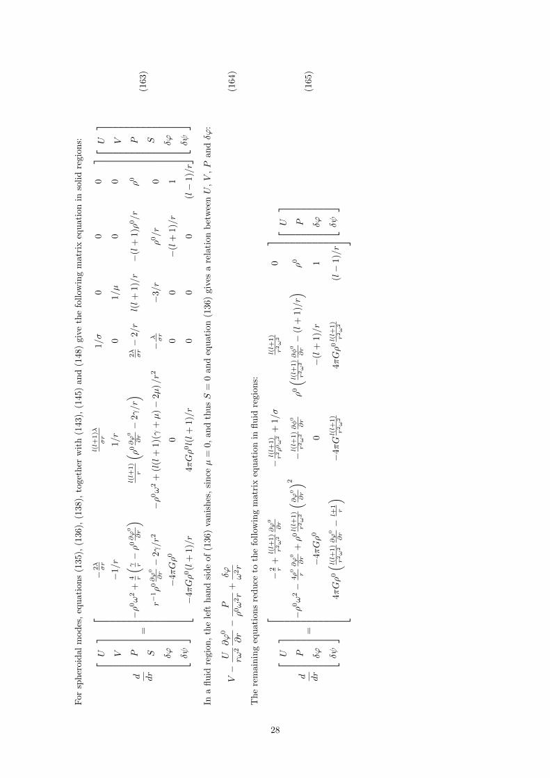
For

sph

eroi

dal

mod

es,

equ

atio

ns

(135

),(1

36),

(138

),to

geth

erw

ith

(143),

(145)

an

d(1

48)

giv

eth

efo

llow

ing

matr

ixeq

uati

on

inso

lid

regio

ns:

d dr

U V P S δϕ δψ

=

−2λσr

l(l+

1)λ

σr

1/σ

00

0

−1/r

1/r

01/µ

00

−ρ

0ω

2+

4 r

( γ r−ρ

0∂ϕ

0

∂r

)l(l+

1)

r

( ρ0∂ϕ

0

∂r−

2γ/r)

2λσr−

2/r

l(l+

1)/r−

(l+

1)ρ

0/r

ρ0

r−1ρ

0∂ϕ

0

∂r−

2γ/r

2−ρ

0ω

2+

(l(l

+1)(γ

+µ

)−

2µ

)/r2

−λ σr

−3/r

ρ0/r

0

−4πGρ

00

00

−(l

+1)/r

1

−4πGρ

0(l

+1)/r

4πGρ

0l(l+

1)/r

00

0(l−

1)/r U V P S δϕ δψ

(1

63)

Ina

flu

idre

gion

,th

ele

fth

and

sid

eof

(136

)va

nis

hes

,si

nceµ

=0,

an

dth

usS

=0

an

deq

uati

on

(136)

giv

esa

rela

tion

bet

wee

nU

,V

,P

an

dδϕ

:

V−

U rω2

∂ϕ

0

∂r−

P

ρ0ω

2r

+δϕ ω2r

(164)

Th

ere

mai

nin

geq

uat

ion

sre

du

ceto

the

foll

owin

gm

atri

xeq

uati

on

infl

uid

regio

ns:

d dr

U P δϕ δψ

=

−2 r

+l(l+

1)

r2ω

2∂ϕ

0

∂r

−l(l+

1)

r2ρ0ω

2+

1/σ

l(l+

1)

r2ω

20

−ρ

0ω

2−

4ρ0

r∂ϕ

0

∂r

+ρ

0l(l+

1)

r2ω

2

( ∂ϕ0 ∂r

) 2−l(l+

1)

r2ω

2∂φ0

∂r

ρ0( l(l+

1)

r2ω

2∂φ0

∂r−

(l+

1)/r)

ρ0

−4πGρ

00

−(l

+1)/r

1

4πGρ

0( l(l+

1)

r2ω

2∂ϕ

0

∂r−

l+1r

)−

4πGl(l+

1)

r2ω

24πGρ

0l(l+

1)

r2ω

2(l−

1)/r U P δϕ δψ

(1

65)

28

To find the eigenfrequencies and eigenfunctions for spheroidal equations is more involved than fortoroidal modes. There are three independent solution vectors of equation (163) that are regular atthe origin. These can be found by examining the exact solutions of equation (163) for a homogeneousEarth, which can be found in chapter 8 of [27].

Using each of these three vectors as an initial value, equation (163) can be integrated to the inner-outer core boundary. Since V is not linearly independent from U , P and δϕ there, only two linearcombinations of these three vectors will satisfy the boundary condition S = 0 at this boundary, say(U1 P1 δϕ1 δψ1

)and

(U2 P2 δϕ2 δψ2

).

These two linear combinations are used as initial value for the solution of equation (165) in theouter core and integrated up to the mantle, leading to two vectors

(U3 0 P3 0 δϕ3 δψ3

)and(

U4 0 P4 0 δϕ4 δψ4

)at the mantle bottom. A linearly independent third starting condition

can be given by(

0 1 0 0 0 0), since in the mantle, V is linearly independent. The third

starting condition allows tangential slip at the core-mantle boundary.

Integrating equation (163) three times through the mantle up to the free surface, three linearly inde-pendent solutions at the surface are now obtained, say

(U5 V5 P5 S5 δϕ5 δψ5

),(

U6 V6 P6 S6 δϕ6 δψ6

)and

(U7 V7 P7 S7 δϕ7 δψ7

). A linear combination of these

vectors obeying the free traction condition at the surface gives the solution for the mode shapes. Hence:

det

P5 P6 P7

S5 S6 S7

ψ5 ψ6 ψ7

= 0 (166)

In general, this will not hold, hence, as with the toroidal modes, this process must be repeatedfor different ω using a root finding algorithm. The solution value of ω is an eigenfrequency and thecorresponding linear combinations of the solution vectors in the various regions yield the correspondingeigenfunctions U , V and δϕ, using equation (164) in the fluid core.

2.5 The excitation problem

2.5.1 Seismic source representation

Earthquakes and other driving forces of the oscillations of the Earth are all characterized by a perma-nent deformation of the Earth at the region where the driving force acts. This means that the linearelastic relationship between stress and strain fails locally and transiently. This idea was introducedby Backus and Mulcahy in 1976. [29]

The failure of the consitutive equations can be represented by a tensor quantity Γij = Γij(~x0, t).

This tensor is called the ‘stress glut’ and is the difference between the model stress given by theconstitutive equation and the real stress in the source region. Both stresses are symmetric hence thestress glut Γij is symmetric as well.

The stress glut vanishes outside the source area, is zero at times before the earthquake and is constantat times after the source has ceased to act. This means that the stress glut rate Γij is zero outsidethe region and time interval of the source.

These considerations lead to a change in the source region of equation (55) to:

ρ0

[∂2si∂t2

+ ∂i(δϕ(~r, t) + sk∂kϕ

0)− (∂ksk)∂iϕ

0

]= ∂j (γijkl∂ksl − Γij) (167)

where we have used the definition (44) of the operator Li. This means Γij is symmetric and

ρ0 ∂2si∂t2− Li (~s) = −∂j (Γij) (168)

Hence the source term can be represented by −∂jΓij . For a point source in space and time the stressglut rate is simply a delta function in space and time:

Γij = Mijδ(~x0 − ~xS)δ(t) (169)

29

where Mij is the moment tensor and ~xS is the source point and the source acts at time t = 0. Notethat since Γij is symmetric, Mij is symmetric as well. Hence 9 independent parameters are needed todescribe a source which is caused by failure of the constitutive equations, six for the moment tensorand three for the location. This means that the source term representation −∂jΓij becomes:

−∂jΓij = −Mij∂jδ(~x0 − ~xS)H(t) (170)

where H(t) is the Heaviside step function.

Failure of the constitutive equation is a process which takes place within the earth, hence no ex-ternal forces play a role. If external forces are taken into account, Γij is not necessarily symmetricanymore, since there are additional, external force terms making up the difference between real stressand model stress. An example of an external force causing an earthquake is a meteorite striking theEarth. For theoretical purposes, the seismogram due to an external force is important, because itallows the calculation of Green’s functions which are of fundamental interest for many seismologicalproblems. Hence a more general source representation, taking into account external point forces is:

−∂jΓij = (fi −Mij∂j)δ(~x0 − ~xS)H(t) (171)

where Mij is not necessarily symmetric. Equation (168) now becomes:

ρ0 ∂2si∂t2− Li (~s) = qiδ(~x

0 − ~xS)H(t) (172)

where qi = qi(~x0, t) = (fi −Mij∂j).

The extra force terms represent a net force acting on the Earth, a non-symmetric moment tensorrepresents an external torque, as can be seen on page 149-150 in [27]. Now 15 parameters are neededto specify this source term, three for the location, three force components and nine moment tensorcomponents. This is the most general point source exerting a net force and torque on the Earth. Weregard the forces and torques applied on the Earth small enough to be able to neglect the effects ofrotation caused by the source. In the next section the synthetic seismogram for this point source willbe calculated.

2.5.2 Synthetic seismograms

The main goal of this chapter is to derive an expression for a synthetic seismogram of the form:

~s(~x0, t

)=∑k

1− eαkt cos(ωkt)

ω2k

∑m

Ekm~smk

(~x0)

(173)

where k is an index incorporating n and l, αk is a parameter governing the attenuation of a modek and Ekm are excitation coefficients of a mode (k,m), dependent on the source parameters. Asdefined earlier, ωk is the angular eigenfrequency of mode k and ~smk is an eigenfunction correspondingto eigenfrequency ωk.

As we have seen in chapter 2.5.1 on the source the seismic displacement ~s at the material particle ~x0

at time t is governed by:

ρ0 ∂2si∂t2− Li (~s) = qiδ(~x

0 − ~xS)H(t) (174)

satisfying boundary conditions (56). In this equation, ρ0 is the unperturbed density distribution, theterms on the right hand size represent a seismic source and L is a linear, self adjoint operator definedin equation (60) having real eigenvalues and orthogonal eigenfunctions in the sense:∫

V 0

ρ0~s ∗k′ · ~skdV 0 = δkk′ (175)

One could object that not all eigenfunctions necessarily have to be orthogonal, since for each l thereare 2l+ 1 degenerate eigenfunctions. Luckily, the eigenfunctions are expanded into (vector) sphericalharmonics, which are orthogonal in the sense:∫ 2π

0

∫ π

0

Y ml (θ, φ)Y m′

l′ (θ, φ) sin θ dθdφ = δll′δmm′ (176)

30

This means that equation (175) certainly holds for all eigenfunctions.

Now a solution of equation (174) is sought in terms of an eigenfunction expansion:

~s(~x0, t) =∑k,m

amk (t)~smk(~x0)

(177)

This is possible because the eigenfunctions of Li form a complete set of basis functions for the dis-placement. We will not prove this fact here, but it stems from the completeness of the vector sphericalharmonic expansion. Substituting (177) in differential equation (174) we find:∑

k,m

ρ0

(∂2amk∂t2

+ ω2amk

)~smk (~x0) = ~qδ(~x0 − ~xS)H(t) (178)

Taking the inner product with ~s ∗k and integrating over V 0, making use of the orthonormality (175)we get:

∂2amk∂t2

+ ω2kamk = Fmk (179)

where

Fmk = Fmk (t) =

∫V 0

(~s ∗mk · ~qδ(~x0 − ~xS)H(t)

)dV 0 (180)

Equation (179) is a differential equation which can be solved by standard methods, for example Laplacetransformation. Its solution is:

amk (t) =1

ωk

∫ t

−∞sin (ωk(t− t′))Fmk (t′)dt′ (181)

assuming that Fmk (t) = amk (t) = 0 for sufficiently small t. Integrating by parts yields:

amk (t) =1

ω2k

∫ t

−∞(1− cos (ωk(t− t′)) Fmk (t′) dt′ (182)

This form is more convenient since Fmk (t) = 0 if the source is inactive. Thus, after the force has ceasedto act:

amk (t) =1

ω2k

∫ ∞−∞

hk(t− t′)Fmk (t′) dt′ (183)

where hk(t) = 1 − cos (ωk(t− t′)). Because attenuation takes place for each mode seperately, theseresults have to be modified to take this effect into account. It appears [22] that it is necessary toreplace hk(t) by:

hk(t) = 1− e−αkt cos(ωkt) (184)

where αk is a decay constant characteristic of mode k. When αk, the eigenfunctions sk and theircorresponding eigenfrequencies ωk are known and the source parameters are known, equation (177)and (183) completely specify the seismogram.

Now let us work out equation (180):

Fmk =

∫V 0

(~s ∗mk · ~qδ(~x0 − ~xS)H(t)

)dV 0

= ~s ∗mk (~xS) · ~qH(t) (185)

Hence Fmk is:

Fmk = ~s ∗mk (~xS) · ~q δ(t) (186)

If this result is used in equation (183) amk (t) becomes:

amk (t) =hk(t)

ω2k

~q · ~s ∗mk (~xS) (187)

31

Using this result in the normal mode expansion (177) we obtain the following expression for theseismogram:

~s(~x0, t) =∑k,m

hk(t)

ω2k

~q · ~s ∗mk (~xS)~smk(~x0)

(188)

Note that this is essentially equation (173) from the beginning of this chapter, where ~q · ~s ∗mk (~x0s) are

the excitation coefficients Ekm. Hence if the excitation coefficients are obtained explicitly in sphericalpolar coordinates we will have an explicit formula to calculate seismograms. The remainder of thischapter is exactly about this subject.

Let us start working out the excitation coefficients. In this derivation ~s ∗ = ~s ∗mk (~xS) to avoid un-clear expressions. For the expression Mij∂js

∗i we need the expression for the gradient of a vector field

in spherical polar coordinates. A straight forward calculation of the gradient of a vector field can befound in [27] appendix A, equation (A.138).

Ekm = ~q · ~s ∗ (189)

= frs∗r + fθs

∗θ + fφs

∗φ

−Mrr∂s ∗r∂r− Mrθ

r

(∂s ∗r∂θ− s ∗θ

)− Mrφ

r

(csc θ

∂s ∗r∂φ− s ∗φ

)−Mθr

∂s ∗θ∂r− Mθθ

r

(∂s ∗θ∂θ

+ s ∗r

)− Mθφ

r

(csc θ

∂s ∗θ∂φ− s ∗φ cot θ

)−Mφr

∂s ∗φ∂r− Mφθ

r

∂s ∗φ∂θ− Mφφ

r

(cot θ

∂s ∗φ∂φ

+ s ∗r + s ∗θ cot θ

)(190)

The next step is to express the eigenfunction ~s ∗mk (~xS) in terms of the eigenfunctions U , V and Wand spherical harmonics, all evaluated at the source. We can combine the results for spheroidal andtoroidal modes if we add for ~s ∗mk equations (153)-(155) with equations (157)-(159) and obtain:

sr(~x) = nUl(r)Yml (θ, φ) (191)

sθ(~x) = nVl(r)∂Y ml (θ, φ)

∂θ+nWl(r) csc θ

∂Y ml (θ, φ)

∂φ(192)

sφ(~x) = nVl(r) csc θ∂Y ml (θ, φ)

∂φ−nWl(r)

∂Y ml (θ, φ)

∂θ(193)

where if the excitation coefficients are to be evaluated for a toroidal mode, U and V have to be put tozero. For a spheroidal mode W = 0. Substituting this expression for ~s ∗mk (~xS) into the expression forthe excitation coefficients and writing U = nUl(rS), V = nVl(rS), W = nWl(rS), Y = Y ml (θS , φS),

Y ′ =[∂Y∂θ

](θ,φ)=(θS ,φS)

, using the fact that ∂Y ∗

∂φ = −imY ∗ and the fact that Y satisfies Legendre’s

equation Y ′′ = − cot θY ′ −(l(l + 1)−m2 csc2 θ

)Y to eliminate Y ′′ and denoting a partial derivative

of U , V , W with respect to r with an overhead dot we obtain:

Ekm = frUY∗ + fθ (V Y ′∗ − im csc θWY ∗)− fφ (im csc θV Y ∗ +WY ′∗)

−MrrUY∗ − Mrθ

r((U − V )Y ′∗ + im csc θWY ∗)

− Mrφ

r(im csc θ (V − U)Y ∗ +WY ′∗)− Mθr

(V Y ′∗ − im csc θWY ∗

)− Mθθ

r

(V(m2 csc2 θ − l(l + 1)

)Y ∗ − V cot θY ′∗ + im csc θW (cot θY ∗ − Y ′∗) + UY ∗

)− Mθφ

r

(−im csc θV Y ′∗ −m2 csc2WY ∗ + im cot θ csc θV Y ∗ + cot θWY ′∗

)+ Mφr

(im csc θV Y ∗ + WY ′∗

)− Mφθ

r

(im cot θ csc θV Y ∗ − im csc θV Y ′∗ +W

(cot θY ′∗ +

(l(l + 1)−m2 csc2 θ

)Y ∗))

− Mφφ

r

(cot θ

(−m2 csc θV Y ∗ + imWY ′∗ + V Y ′∗ − im csc θWY ∗

)+ UY ∗

)(194)

32

Rearranging terms, we obtain:

Ekm = Y ∗(frU −MrrU + l(l + 1)

Mθθ

rV − Mθθ +Mφφ

rU − Mφθ

rl(l + 1)W

)+(cot θY ′∗ −m2 csc2 θY ∗

)(Mθθ

rV − Mθφ +Mφθ

rW

)+ cot θ

(m2 csc θY ∗ − Y ′∗

)Mφφ

rV

+ Y ′∗(fθV − fφW −

Mrθ

r(U − V )− Mrφ

rW −MθrV +MφrW

)− im csc θY ∗

(fθW + fφV +

Mrθ

rW +

Mrφ

r(V − U)−MθrW −MφrV

)− im csc θ (cot θY ∗ − Y ′∗)

(Mθθ

rW +

Mθφ +Mφθ

rV

)− im cot θ (Y ′∗ − csc θY ∗)

Mφφ

rW (195)

The idea is now to put the source in the north pole (θS = 0). This will simplify the expression forEkm greatly. Since we have a non-rotating Earth, where the poles are on the axis of rotation, this isnot a problem. To do this, we take the limit of the expression above as the source point approachesthe pole along the meridian φ = 0. It is important to define a meridian along which we approach thepole, because the unit vector φ will tend to different limits allong different meridians. This all stemsfrom the fact that the unit vectors θ and φ are not well defined at the pole.

Now we take the limits of the terms depending on the angular coordinates, for φS = 0. This meansthat the unit vectors (r, θ, φ) and the source direction (in the components of the force vector fi andmoment tensor Mij), point in the directions (up, south, east):

limθS→0

Y ∗ =

ν if m = 00 if m = ±10 if m = ±2

(196)

limθS→0

(cot θY ′∗ −m2 csc2 θY ∗

)=

−νζ2/2 if m = 00 if m = ±1

−νζ√ζ2 − 2/4 if m = ±2

(197)

limθS→0

cot θ(m2 csc θY ∗ − Y ′∗

)=

νζ2/2 if m = 00 if m = ±1

νζ√ζ2 − 2/4 if m = ±2

(198)

limθS→0

Y ′∗ =

0 if m = 0∓νζ/2 if m = ±10 if m = ±2

(199)

limθS→0

−im csc θY ∗ =

0 if m = 0iνζ/2 if m = ±10 if m = ±2

(200)

limθS→0

−im csc θ (cot θY ∗ − Y ′∗) =

0 if m = 00 if m = ±1

±iνζ√ζ2 − 2/4 if m = ±2

(201)

limθS→0

−im cot θ (Y ′∗ − csc θY ∗) =

0 if m = 00 if m = ±1

∓iνζ√ζ2 − 2/4 if m = ±2

(202)

In these expressions, ν =√

2l+14π and ζ2 = l(l + 1). For |m| > 2 all limits tend to zero, hence if the

limits are put into the expression for the spherical harmonic coefficients, we obtain after reworking

33

some terms:

Ekm =

ν(frUk −MrrUk +

((V ζ2 − 2U)/2rS

)(Mθθ +Mφφ)

+(Wζ2/2rS

)(Mθφ −Mφθ)

)if m = 0

νζ2

((V ∓ iW )(∓fθ + ifφ) + (V ∓ iW )(±Mθr − iMφr)

+ (U − V ± iW )(±Mrθ − iMrφ)/rS

)if m = ±1

νζ√ζ2−2

4rS(V ∓ iW )(Mφφ −Mθθ ± iMθφ ± iMφθ) if m = ±2

(203)

In this expression, the θ-direction corresponds to the south, the φ-direction is east, because we choseφ = 0 as our approaching meridian.

Of course, for practical reasons, it is not really useful to have an expression for a seismogram withthe source at the North pole, since you want to be able to produce a seismogram with an arbitrarysource location. The easiest way to solve this problem is to define a new spherical polar coordinatesystem, the epicentral coordinate system, with the source location as the north pole. The colatitudethen becomes the angular epicentral distance between the source and receiver, the longitude is theazimuth to the receiver, measured in counterclockwise sense from due south at the source. Moreabout the epicentral coordinate system can be found in [27], Chapter 10.1. I will now state the resultsexpressing the epicentral distance Θ and azimuth Φ in terms of the source location (rS , θS , φS) andreceiver location (r, θ, φ) in ordinary spherical polar coordinates.

cos Θ = sin θS sin θ cos(φS − φ) + cos θS cos θcos Φ = csc Θ (cos θS sin θ cos(φ− φS)− sin θS cos θ)sin Φ = csc Θ sin θ sin(φ− φS)

(204)

The seismograms sΘ and sΦ produced with this coordinate system are in the longitudinal and trans-verse direction respectively. If we want to calculate seismograms in the northern and eastern directionwe just have to apply a rotation to the results:

sN = −sΘ cos ξ − sΦ sin ξ (205)

sE = −sΘ sin ξ + sΦ cos ξ (206)

where subscripts N and E refer to the components in the directions North and East and where ξ isthe conventional azimuth of the source from the receiver:

cos ξ = csc Θ (cos θS sin θ − sin θS cos θ cos(φ− φS))sin ξ = csc Θ sin θS sin(φS − φ)

(207)

Now all ingredients for the calculation of a synthetic seismogram on a SNREI earth have been assem-bled. In the Results chapter the computational procedure is discussed and one example calculationis presented and will be compared to real data and other synthetic seismograms in the Discussionsection.

3 Results

In this chapter, a description of the numerical procedure used to calculate synthetic seismograms isgiven, together with the resulting synthetic seismograms and real data acquired from the seismographat Fort Hoofddijk, Utrecht to be able to make a comparison between the theory and reality.

To do this, one particular event is analyzed, the 9.0 MW earthquake on 11-03-2011 near the eastcoast of Honshu, Japan has been chosen. This event, which had a very destructive impact on Japan,caused maximum displacements in the Netherlands of approximately 1 centimeter.

Many moment tensor inversions have been performed for this earthquake, I use the USGS Centroid

34

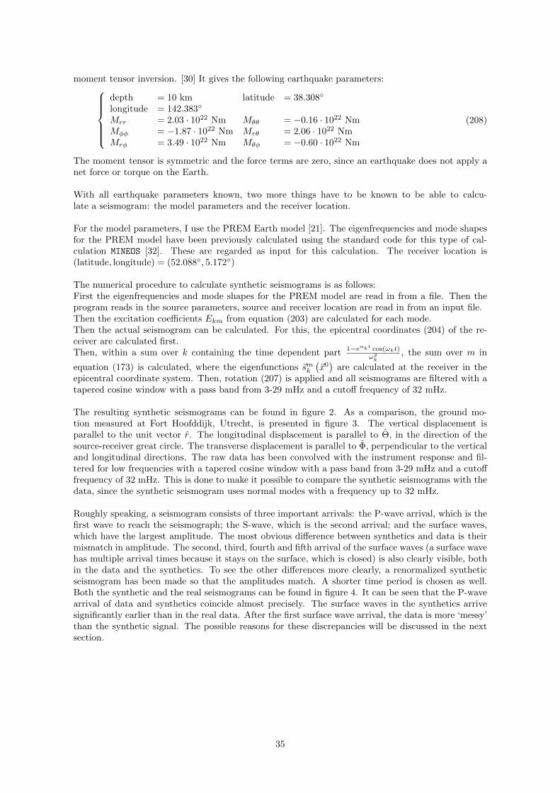
moment tensor inversion. [30] It gives the following earthquake parameters:depth = 10 km latitude = 38.308◦

longitude = 142.383◦

Mrr = 2.03 · 1022 Nm Mθθ = −0.16 · 1022 NmMφφ = −1.87 · 1022 Nm Mrθ = 2.06 · 1022 NmMrφ = 3.49 · 1022 Nm Mθφ = −0.60 · 1022 Nm

(208)

The moment tensor is symmetric and the force terms are zero, since an earthquake does not apply anet force or torque on the Earth.

With all earthquake parameters known, two more things have to be known to be able to calcu-late a seismogram: the model parameters and the receiver location.

For the model parameters, I use the PREM Earth model [21]. The eigenfrequencies and mode shapesfor the PREM model have been previously calculated using the standard code for this type of cal-culation MINEOS [32]. These are regarded as input for this calculation. The receiver location is(latitude, longitude) = (52.088◦, 5.172◦)

The numerical procedure to calculate synthetic seismograms is as follows:First the eigenfrequencies and mode shapes for the PREM model are read in from a file. Then theprogram reads in the source parameters, source and receiver location are read in from an input file.Then the excitation coefficients Ekm from equation (203) are calculated for each mode.Then the actual seismogram can be calculated. For this, the epicentral coordinates (204) of the re-ceiver are calculated first.Then, within a sum over k containing the time dependent part 1−eαkt cos(ωkt)

ω2k

, the sum over m in

equation (173) is calculated, where the eigenfunctions ~smk(~x0)

are calculated at the receiver in theepicentral coordinate system. Then, rotation (207) is applied and all seismograms are filtered with atapered cosine window with a pass band from 3-29 mHz and a cutoff frequency of 32 mHz.

The resulting synthetic seismograms can be found in figure 2. As a comparison, the ground mo-tion measured at Fort Hoofddijk, Utrecht, is presented in figure 3. The vertical displacement isparallel to the unit vector r. The longitudinal displacement is parallel to Θ, in the direction of thesource-receiver great circle. The transverse displacement is parallel to Φ, perpendicular to the verticaland longitudinal directions. The raw data has been convolved with the instrument response and fil-tered for low frequencies with a tapered cosine window with a pass band from 3-29 mHz and a cutofffrequency of 32 mHz. This is done to make it possible to compare the synthetic seismograms with thedata, since the synthetic seismogram uses normal modes with a frequency up to 32 mHz.

Roughly speaking, a seismogram consists of three important arrivals: the P-wave arrival, which is thefirst wave to reach the seismograph; the S-wave, which is the second arrival; and the surface waves,which have the largest amplitude. The most obvious difference between synthetics and data is theirmismatch in amplitude. The second, third, fourth and fifth arrival of the surface waves (a surface wavehas multiple arrival times because it stays on the surface, which is closed) is also clearly visible, bothin the data and the synthetics. To see the other differences more clearly, a renormalized syntheticseismogram has been made so that the amplitudes match. A shorter time period is chosen as well.Both the synthetic and the real seismograms can be found in figure 4. It can be seen that the P-wavearrival of data and synthetics coincide almost precisely. The surface waves in the synthetics arrivesignificantly earlier than in the real data. After the first surface wave arrival, the data is more ‘messy’than the synthetic signal. The possible reasons for these discrepancies will be discussed in the nextsection.

35

0 5000 10000 15000 20000 25000 30000Time (s)

-0.1

-0.05

0

0.05

0.1

Ver

tical

dis

plac

emen

t (m

)

(a) Vertical displacement

0 5000 10000 15000 20000 25000 30000Time (s)

-0.08

-0.06

-0.04

-0.02

0

0.02

0.04

0.06

0.08

Long

itudi

nal d

ispl

acem

ent (

m)

(b) Longitudinal displacement

0 5000 10000 15000 20000 25000 30000Time (s)

-0.05

0

0.05

Tra

nsve

rse

disp

lace

men

t (m

)

(c) Transverse displacement

Figure 2: Synthetic displacement at Fort Hoofddijk, Utrecht in meters. The time at the origin is thetime of the event.

36

0 5000 10000 15000 20000 25000 30000Time (s)

-0.02

-0.01

0

0.01

0.02

Ver

tical

dis

plac

emen

t (m

)

(a) Vertical displacement

0 5000 10000 15000 20000 25000 30000Time (s)

-0.01

0

0.01

Long

itudi

nal d

ispl

acem

ent (

m)

(b) Longitudinal displacement

0 5000 10000 15000 20000 25000 30000Time (s)

-0.02

-0.01

0

0.01

0.02

Tra

nsve

rse

disp

lace

men

t (m

)

(c) Transverse displacement

Figure 3: Displacement at Fort Hoofddijk, Utrecht in meters. The time at the origin is the time ofthe event.

37

0 1000 2000 3000Time (s)

-0.02

-0.01

0

0.01

0.02

Ver

tical

dis

plac

emen

t (m

)

(a) Vertical displacement

0 1000 2000 3000Time (s)

-0.02

-0.01

0

0.01

0.02

Long

itudi

nal d

ispl

acem

ent (

m)

(b) Longitudinal displacement

0 1000 2000 3000Time (s)

-0.02

-0.01

0

0.01

0.02

Tra

nsve

rse

disp

lace

men

t (m

)

(c) Transverse displacement

Figure 4: Displacement at Fort Hoofddijk, Utrecht in meters. The time at the origin is the time ofthe event.

38

4 Discussion

The outline of this section is as follows. First a very short description of this study will be given,followed with a discussion of the results. Then the importance of synthetic seismograms will be dis-cussed, and directions of further research will be given.

The main goal of this study is to give an introduction into the theory of normal mode seismologyfrom first principles. For this, the free oscillations of a spherically symmetric, non-rotating, elasticand isotropic earth are obtained. The excitation problem is also discussed and an expression for atheoretical seismogram for a point source is derived. As an application, this expression is used togenerate a synthetic seismogram for the 9.0 MW earthquake on 11-03-2011 near the east coast ofHonshu, Japan. This synthetic seismogram is compared with real data.

The main difference between synthetics and data is their amplitude. The amplitude of the syn-thetics is approximately 6 times bigger than the amplitude of the data. The wave form is much betterin agreement, the P-wave arrival at 1300 seconds is however better in agreement than the surfacewave arrival, for which the arrival time in the theoretical seismogram is earlier, at 2400 seconds. Thereal data show an arrival time of the surface waves at approximately 2550 seconds. The theoreticalseismogram is also less noisy after the surface wave arrival.

The difference in amplitude is something you would not expect, since the moment tensor compo-nents are determined with an inversion technique using similar expressions for the seismogram as theone used in this study. It might have something to do with the specific earthquake chosen. Becausethe event was very big, it might be that the point source approximation is not valid anymore. Now allenergy emerges from one point, it might very well be that the amplitude of the synthetic seismogramwould be lower if the earthquake energy was spread over a larger source area by taking for examplemore point sources in the earthquake region replacing the single point source used in this study.

It is quite certain that the mismatch in amplitude is not a numerical issue, since another programexists (apsyn) [33], doing the same calculation, giving the same amplitude. This can be seen in figure5. The reason the signal obtained from apsyn is more noisy and has a bigger amplitude is that thesignal obtained from this study has been filtered more. But most importantly, the amplitudes are inthe same order of magnitude.

A possible explanation for the difference in P-wave arrival match with the surface wave match is theSNREI model: it is not laterally heterogeneous. Since the surface waves are trapped on the Earth’ssurface, which is not homogeneous at all, differences with the mean homogeneous earth occur quickly.The surface waves arriving in the Netherlands from Japan mostly travel through continental litho-sphere, in which the surface wave speed is lower than in oceanic lithosphere, because of the lowerdensity of the continental lithosphere. The P-waves travel through the deeper mantle, which is lessheterogeneous than the crust and therefore the arrival times match better.

A reason for other differences between the real data and the synthetics is the fact that after theJapan earthquake many strong aftershocks took place, which were significantly lower in magnitude,but which could be the explanation for the noise in the data, which lacks in the synthetic seismogram.

The importance of synthetic seismograms for seismology is its application in the solution of inverseproblems. By comparing synthetic seismograms with real data, the misfit between the two originatesfrom deviations of the model and source parameters from the real Earth situation. The misfit canbe defined in several ways. One could define the misfit in the frequency domain for the eigenfre-quencies of the Earth. Another common way of defining misfit is to take the difference between thesynthetic seismogram and the real data, square it and integrate it over the entire seismogram. Of-ten, certain portions of the seismogram are taken. For example, one can take the mismatch of theP-wave arrival times, S-wave arrival times, amplitude or surface waves. As soon as the misfit is de-fined, the challenge is to find an inverse operation which can be performed on the misfit to obtain themodel which minimalizes the misfit. An example of the solution of such a problem can be found in [34].

39

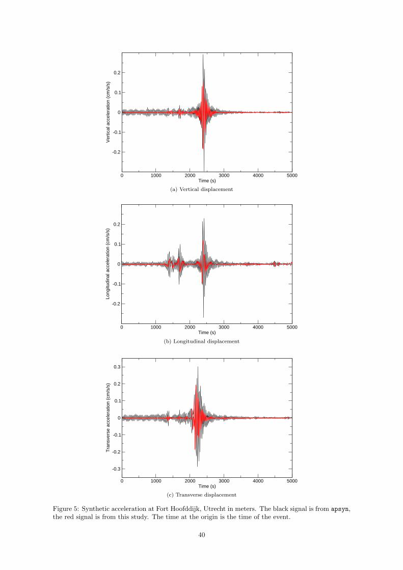
0 1000 2000 3000 4000 5000Time (s)

-0.2

-0.1

0

0.1

0.2

Ver

tical

acc

eler

atio

n (c

m/s

/s)

(a) Vertical displacement

0 1000 2000 3000 4000 5000Time (s)

-0.2

-0.1

0

0.1

0.2

Long

itudi

nal a

ccel

erat

ion

(cm

/s/s

)

(b) Longitudinal displacement

0 1000 2000 3000 4000 5000Time (s)

-0.3

-0.2

-0.1

0

0.1

0.2

0.3

Tra

nsve

rse

acce

lera

tion

(cm

/s/s

)

(c) Transverse displacement

Figure 5: Synthetic acceleration at Fort Hoofddijk, Utrecht in meters. The black signal is from apsyn,the red signal is from this study. The time at the origin is the time of the event.

40

The main direction of further research is the application of normal mode synthetic seismograms ininverse problems, to obtain a more detailed picture of the Earth’s interior. Because nowadays moreadvanced codes exist for calculating synthetic seismograms, this relatively simple way of calculatingsynthetics for a SNREI Earth can be used as a starting point in the development of an inverse method,since calculations can be done quickly. A more specific research direction is to find out why such a bigamplitude difference between data and synthetics exists in this particular study. The same comparisonhas to be made for a smaller and less powerful source to see whether the cause is indeed the failure ofthe point source approximation.

Regarding the calculation of synthetic seismograms, of course it is possible to do better than theresult presented in this study. Important effects that are neglected such as the rotation and ellipticityof the Earth, which causes splitting in de 2l+ 1 modes corresponding to each set of modes (n, l). Lat-eral heterogeneity and non hydrostatic initial stress will also change the results, as well as anisotropy.There are codes currently available taking this into account, but a discussion of the theory behindthese codes was not the aim of this study.

5 Conclusions

The conclusions of this study can be split in two categories: conclusions regarding the theory of thenormal modes of oscillation of the Earth and the theoretical expression of a seismogram and conclu-sions about the application of the expression of a seismogram on the 9.0 MW earthquake on 11-03-2011near the east coast of Honshu, Japan.

To find the normal modes of oscillation of the Earth, the normal modes of a spherically symmetric, non-rotating, elastic and isotropic Earth model (SNREI) are discussed. A linear differential equation forfree oscillations with small displacements ~s is derived which has the form Li (~s) = ρ0

(~x0, t

)∂2t si(~x0, t

),

where Li is a linear, self adjoint operator acting on the displacement field ~s, depending only on knownmodel parameters. The equilibrium density distribution is given by ρ0, ∂2

t denotes the second partialderivative with respect to time.

This equation is solved in spherical coordinates, with a vector spherical harmonic expansion of thedisplacement, under boundary conditions of continuous traction on all interfaces of the model andzero traction on the surface. Displacement is continuous everywhere, except at fluid-solid boundarieswhere displacement tangential to the boundary can be discontinuous.

The differential equations allow two types of normal modes: toroidal oscillations in which the motionis perpendicular to straight lines through the center of the Earth. The other type of oscillations arecalled spheroical oscillations in which both radial and tangential motion exists. All separate modesare completely decoupled from each other.

If all normal modes of the Earth have been determined, any seismogram can be obtained by per-forming a normal mode sum in which the coefficient for each mode is determined by the seismicsource. The seismic source can be represented by a force fi and a moment tensor Mij in the case ofa point source. For an earthquake, fi = 0 and Mij is symmetric. The expression for a seismogram is:

~s(~x0, t

)=∑k

1− eαkt cos(ωkt)

ω2k

∑m

Ekm~smk

(~x0)

(209)

where ~s(~x0, t) is the displacement as a function of the position of a particle initially at ~x0 at time t.Indices k and m are numbers identifying separate modes, αk is a constant determining the decay of amode (k,m). The eigenfrequency of mode (k,m) is given by ωk. The excitation coefficient for a mode(k,m) is given by Ekm and is determined by the source. The displacement of a normal mode (k,m)is given by ~smk .

The synthetic seismogram calculated for the earthquake in Japan has generally the same waveformas the real data. There are however some remarkable differences. The amplitude of the theoreticalseismogram is approximately 6 times bigger than the amplitude of the data. The arrival time of the

41

surface waves is earlier in the theoretical seismogram, but the P-wave arrival times coincide.

Possible explanations for these differences are the scale of the event and the heterogeneity of thelithosphere. Because the Japan earthquake was an event which did not occur at a point, but in alarger region, the point source approximation might not be valid. This is why the equivalent pointsource might produce such large amplitudes, because all the energy is released at one instant and atone point. The path between Japan and the Netherlands consists mostly of continental lithosphere.In continental lithosphere, the surface wavespeed is relatively slow, which explains the late arrivaltime of the real surface wave signal relative to the synthetics. Because P-waves travel through themantle, which is less heterogeneous than the crust, the P-wave arrival time misfit is small.

The normal modes of the Earth can be used to tackle inverse problems regarding the structure ofthe Earth or the description of an earthquake source. Programs are available to calculate more pre-cise synthetic seismograms which take into account more Earth model features, such as rotation,ellipticity and lateral heterogeneity, but these are impractical if a new inverse technique is developedbecause of the long calculation time. Synthetic seismograms calculated with the expressions in thisstudy have as main advantage that a relatively accurate synthetic seismogram can be generated in acouple of seconds. Besides, the theory presented in this study is a good introduction in normal modeseismology and prepares for the next step in the theory: the breaking of the spherical symmetry ofthe Earth.

References

[1] J. H. Woodhouse, Lecture notes, obtained from Jeannot Trampert

[2] A. M. Dziewonski and J. H. Woodhouse, Studies of the seismic source using normal-mode theory.In Kanamori, H. and Boschi, E., editors, Earthquakes: observation, theory, and interpretation:notes from the International School of Physics “Enrico Fermi” (1982: Varenna, Italy), pages45-137. North-Holland Publ. Co., Amsterdam., 1983.

[3] USGS, FAQs at http://earthquake.usgs.gov

[4] S. D. Poisson, 1829 Memoire sur l’equilibre et le mouvement des corps elastiques, Mem. Acad.Roy. Sci. Inst. France, 8, 357-570.

[5] W. Thomson, 1863 On the rigidity of the Earth, Phil. Trans. Roy. Soc. Lond., 153, 573-582.

[6] W. Thomson, 1863 Dynamical problems regarding elastic spheroidal shells and spheroids of in-compressible liquid, Phil. Trans. Roy. Soc. Lond., 153, 583-616.

[7] H. Lamb, 1882, On the vibrations of an elastic sphere, Proc. Lond. Math. Soc., 13, 189-212.

[8] J. W. S. Rayleigh, 1906, On the dilatational stability of the Earth, Proc. Roy. Soc. Lond., Ser.A, 77,486-499.

[9] A. E. H. Love, 1907, The gravitational stability of the Earth, Phil. Trans. Roy. Soc. Lond., Ser.A, 207, 171-241.

[10] A. E. H. Love, 1911, Some Problems of Geodynamics, Cambridge University Press, Cambridge.Reprinted in 1967 by Dover Publications, New York.

[11] L. M. Hoskins, 1920, The strain of a gravitating sphere of variable density and elasticity, Trans.Am. Math. Soc., 21, 1-43.

[12] J. H. Jeans, 1927, The propagation of earthquake waves, Proc. Roy. Soc. Lond., Ser. A, 102,554-574.

[13] N. Jobert, 1956, Evaluation de la periode d’oscillation d’une sphere heterogene, par applicationdu principe de Rayleigh, Comptes Rendus Acad. Sci. Paris, 243, 1230-1232.

[14] N. Jobert, 1957, Sur la periode propre des oscillations spheroıdales de la Terre, Comptes RendusAcad. Sci. Paris, 244, 921-922.

42

[15] N. Jobert, 1961, Calcul approche de la periode des oscillations spheroıdales de la Terre, Geophys.J. Roy. Astron. Soc., 4, 242-258.

[16] C. L. Pekeris and H. Jarosch, 1958, The free oscillations of the Earth. In Benioff, H., Ewing, M.,Howel, Jr., B.F. & Press, F., editors, Contributions in Geophysics in Honor of Beno Gutenberg,pages 171-192, Pergamon, New York.

[17] H. Takeuchi, 1959, Torsional oscillations of the Earth and some related problems, Geophys. J.Roy. Astron. Soc., 2, 89-100.

[18] Z. Alterman, H. Jarosch and C. L. Pekeris, 1959, Oscillations of the Earth, Proc. Roy. Soc. Lond.,Ser. A, 252, 80-95.

[19] C. L. Pekeris, Z. Alterman and H. Jarosch, 1961, Comparison of theoretical with observed valuesof the periods of the free oscillations of the Earth, Proc. Nat. Acad. Sci. USA, 47, 91-98.

[20] F. Gilbert and A. M. Dziewonski, 1975, An application of normal mode theory to the retrieval ofstructural parameters and source mechanisms from seismic spectra, Phil. Trans. Roy. Soc. Lond.,Ser. A, 278, 187-269.

[21] A. M. Dziewonski and D. L. Anderson, 1981, Preliminary reference Earth model, Phys. EarthPlanet. Int., 25, 297-356.

[22] F. Gilbert, 1970, Excitation of the normal modes of the Earth by earthquake sources, Geophys.J. Roy. Astron. Soc., 22, 223-226.

[23] B. V. Kostrov, 1970, The theory of the focus for tectonic earthquakes, Izv. Bull. Akad. Sci. USSR,Phys. Solid Earth, 4, 84-101.

[24] A. M. Dziewonski, T.-A. Chou and J. H. Woodhouse, 1981, Determination of earthquake sourceparameters from waveform data for studies of global and regional seismicity, J. Geophys. Res.,86, 2825-2852.

[25] K. Aki and P. G. Richards, 2002, Quantitative Seismology, Chapter 2.1, University Science Books,California, Second Edition.

[26] W. S. Slaughter, 2002, The linearized theory of elasticity, page 51, Birkhauser Boston.

[27] F. A. Dahlen and J. Tromp, 1998, Theoretical Global Seismology, Princeton University Press,Princeton, New Jersey.

[28] P. M. Morse and H. Feshbach, 1953, Methods of Theoretical Physics, pp 1898-1901, McGraw-Hill.

[29] G. E. Backus and M. Mulcahy, 1976, Moment tensors and other phenomenological descriptionsof seismic sources, Geophys. J. Roy. Astron. Soc., 46, 341-361 and Geophys. J. Roy. Astron. Soc.,47, 301-329.

[30] The earthquake data can be obtained at:http://earthquake.usgs.gov/earthquakes/eqinthenews/2011/usc0001xgp/

[31] The animations can be obtained at:http://icb.u-bourgogne.fr/nano/MANAPI/saviot/terre/index.en.html

[32] The program can be obtained at the following internet address:http://www.geodynamics.org/cig/software/mineos/

[33] A computer program made by John Woodhouse in the seventies. Obtained from Jeannot Trampertat the University of Utrecht.

[34] J. Tromp, C. Tape and Q. Liu, 2005, Seismic Tomography, Adjoint Methods, Time Reversal, andBanana-Doughnut Kernels, Geophysical Journal International, Vol. 160, Issue 1, 195-216.

43