arX

iv:q

uant

-ph/

0608

206v

4 2

8 A

pr 2

008

Santa Fe Institute Working Paper 06-09-031arxiv.org/quant-ph/0608206

Computation in Finitary Stochastic and Quantum Processes

Karoline Wiesner1, 2, ∗ and James P. Crutchfield1, 2, †

1Complexity Sciences Center and Physics Department,University of California Davis, One Shields Avenue, Davis, CA 95616

2Santa Fe Institute, 1399 Hyde Park Road, Santa Fe, NM 87501(Dated: November 16, 2017)

We introduce stochastic and quantum finite-state transducers as computation-theoretic modelsof classical stochastic and quantum finitary processes. Formal process languages, representing thedistribution over a process’s behaviors, are recognized and generated by suitable specializations. Wecharacterize and compare deterministic and nondeterministic versions, summarizing their relativecomputational power in a hierarchy of finitary process languages. Quantum finite-state transducersand generators are a first step toward a computation-theoretic analysis of individual, repeatedlymeasured quantum dynamical systems. They are explored via several physical systems, includingan iterated beam splitter, an atom in a magnetic field, and atoms in an ion trap—a special case ofwhich implements the Deutsch quantum algorithm. We show that these systems’ behaviors, and sotheir information processing capacity, depends sensitively on the measurement protocol.Keywords: stochastic process, information source, transducer, quantum machine, formal language,quantum computation

PACS numbers: 05.45.-a 03.67.Lx 03.67.-a 02.50.-r 89.70.+c

Contents

I. Introduction 1A. Finite Quantum Computing 2B. Dynamics, Information, and Measurement 2C. Technical Setting 2D. Overview 3

II. Finitary Stochastic Processes 3

III. Stochastic Transducers 4A. Definition 5B. Graphical Representation 5C. Word Probabilities 5

IV. Stochastic Recognizers and Generators 6A. Stochastic Recognizers 6B. Stochastic Generators 8C. Properties 9

V. Finitary Quantum Processes 10A. Quantum States 10B. Quantum Measurement 11

VI. Quantum Transducers 11A. Definition 11B. Measurement 12C. Evolution and Word Distributions 12D. Properties 12

VII. Quantum Recognizers and Generators 13A. Quantum Recognizers 13

∗Electronic address: k.wiesner@bristol.ac.uk†Electronic address: chaos@cse.ucdavis.edu

B. Alternatives 14C. Quantum Generators 14

D. Properties 15

E. Finitary Process Hierarchy 16

VIII. Quantum Generators and Finitary

Processes: Examples 17A. Two-State Quantum Processes 17

1. Iterated Beam Splitter 17B. Three-State Quantum Processes 19

1. Golden Mean Quantum Machine 19

2. Quantum Even Process 19C. Four-State Quantum Process 20

1. Quantum Transducer for Trapped Ions 202. Deutsch Algorithm as a Special Case 22

IX. Concluding Remarks 23

Acknowledgments 24

References 24

I. INTRODUCTION

Automata theory is the study of abstract computingdevices, or machines, and the class of functions they canperform on their inputs. In the 1940’s and 1950’s, simplekinds of machines, so-called finite-state automata, wereintroduced to model brain function [1, 2]. They turnedout to be extremely useful for a variety of other pur-poses, such as studying the lower limits of computationalpower and synthesizing logic controllers and communi-cation networks. In the late 1950’s, the linguist NoamChomsky developed a classification of formal languages

2

in terms of the grammars and automata required to rec-ognize them [3]. On the lowest level of Chomsky’s hi-erarchy, for example, whether or not a given sentenceobeys the grammatical rules of a language is answeredby a finite-state automaton.Our understanding of the nature of computing has

changed substantially in the intervening half century. Inrecent years the study of computation with elementarycomponents that obey quantum mechanical laws has de-veloped into a highly active research area.

A. Finite Quantum Computing

The physical laws underlying quantum computationare a mixed blessing. On the one hand, a growing bodyof theoretical results suggests that a computational de-vice whose components are directly governed by quantumphysics may be considerably more powerful than its clas-sical counterpart. Undoubtedly, the most celebrated ofthese results is Shor’s factoring algorithm from 1994 [4].Other results include Grover’s quantum search algorithmfrom 1996 [5]. On the other hand, the results employpowerful computational architectures, such as quantumTuring machines [6], that are decidedly more powerfulthan finite-state machines and that must maintain highdegrees of internal coherence and environmental isolationduring operation. For a review of theoretical and experi-mental studies of quantum computation see, for example,Refs. [7, 8].However, to date, implementation efforts have fallen

substantially short of the theoretical promise. So far ex-perimental tests of quantum computation are on small-scale systems—in fact, very small. Currently, the largestcoherent system of information storage supports only 7quantum bits or qubits [9]. Thus, the study of finite-statequantum automata is motivated by very practical con-cerns. They reflect the capabilities of currently feasiblequantum computers. As was also true in the first days ofdigital computers, though, the study of finite machines isalso a starting point, here for developing a computationalhierarchy for quantum dynamical systems.

B. Dynamics, Information, and Measurement

A common goal in the practice of quantum theory is topredict the expectation of outcomes from an ensemble ofisolated measurements. There is a key difference, though,between this and what one needs to understand quan-tum processes. For quantum processes, such as found inmolecular dynamics, one must analyze behavior ; predict-ing an observable’s mean value is insufficient.Quantum mechanics can be extended, of course, to ad-

dress behavior. This has been done in rather generalframeworks (e.g., Ref. [10]), as well as in special cases,such as quantum Markov chains [11]. However, ques-tions about a quantum system’s information processing

capacity remain unanswered. For example, how much ofa quantum system’s history is stored in its state? Howis that information processed to produce future behav-ior? More pointedly, even if a system is designed to havea desired information processing capacity, the questionalways remains whether or not that capacity is actuallyused during operation.An intriguing, but seemingly unrelated area of research

in quantum behavior is quantum chaos—the productionof information through the exponential amplification ofperturbations [12]. Since any quantum system is de-scribed by the Schrodinger equation, which is linear,chaotic behavior cannot arise. However, quantum sys-tems that exhibit chaotic behavior in the classical limitcan show signatures of chaos in semi-classical regimes.Thus, analyzing the relationship between classical andquantum dynamical systems plays an important role inunderstanding the origins of quantum information pro-duction.For quantum systems, in contrast with their classi-

cal counterparts, including measurement interactions isessential to any complete description. Unfortunately,this is largely missing from current dynamical theories.Nonetheless, simulation studies show that measurementinteractions lead to genuinely chaotic behavior in quan-tum dynamical systems, even far from the semi-classicallimit [13]. Observation must be the basis for modelinga quantum process—either in describing its behavior orquantifying its computational capacity.

C. Technical Setting

Here we introduce finite computation-theoretic quan-tum models that, when analyzed with tools from quan-tum mechanics and stochastic processes, simultaneouslyembody dynamics, measurement, and information pro-cessing. Studies of quantum chaos are, in effect, exten-sions of the theory of nonlinear (classical) dynamics. Dy-namical systems are often analyzed by transforming theminto finite-state automata using the methods of symbolicdynamics [14]. The quantum automata in the followingmodel dynamical behavior and include measurement in-teractions and so provide a kind of symbolic dynamics forquantum systems [15]. The result is a line of inquiry com-plementary to both quantum computation and quantumdynamical systems.One goal is to develop a representation of quantum

processes that allows one to analyze their intrinsic com-putation. Intrinsic computation in a dynamical systemis an inherent property of the behavior the system gen-erates [16]. One asks three basic questions of the system:First, how much historical information is stored in thecurrent state? Second, in what architecture is that in-formation stored? Finally, how is the stored informationtransformed to produce future behavior? This approachhas been used to analyze intrinsic computation in clas-sical dynamical systems, statistical mechanical systems,

3

and stochastic processes [17, 18, 19, 20].We view the present contribution as a direct extension

of this prior work and, also, as complementary to thecurrent design and theoretical-engineering approach toquantum computation. Specifically, we focus on the dy-namics of quantum processes, rather than on methods toconstruct devices that implement a desired function. Weexpress the intrinsic information processing using variouskinds of finite-memory devices. We emphasize the effectsof measurement on a quantum system’s behavior and so,in this way, provide a somewhat different view of quan-tum dynamical systems for which, typically, observationis ignored. An information-theoretic analysis using theresulting framework can be found in Refs. [15, 21].Most directly, we are interested, as natural scientists

are, in behavior—how a system state develops over time.In the computation-theoretic setting this translates intoa need to model generators. In contrast, the conven-tional setting for analyzing the computational power ofautomata centers around detecting membership of wordsin a language. As a consequence, the overwhelming frac-tion of existing results on automata concerns devices thatrecognize an input string—and on problems that can berecast as such. Automata that spontaneously generateoutputs are much less often encountered, if at all, inthe theory of computation. Nonetheless, generators arenecessary if one wants to model physical processes usingdynamical systems. In particular, as we hope to show,quantum generators are a key tool for detecting informa-tion processing capabilities inherent in natural processes.

D. Overview

Due to the range of topics, in the following we give aselective, but self-contained treatment. We review whatis needed from automata, formal languages, and quan-tum theory, though familiarity with those areas is helpful.Citations to reference texts are given at the appropriatepoints.Our approach will make most sense, especially to those

unfamiliar with the theory of formal languages, if we de-vote some time to reviewing basic automata theory andits original goals. This also allows us to establish, in agraded fashion, the necessary notation for the full devel-opment, clearly identifying which properties are quantummechanical and which, in contrast, are essentially classi-cal (and probabilistic). In addition, this illustrates oneof the principle benefits of discrete computation theory:i.e., the classification of devices that implement differ-ent kinds of information processing. Those for whomautomata and formal languages are well known, though,should appreciate by the end of the review the physicaland dynamical motivations, since these will be expressedwithin the existing frameworks of discrete computationand stochastic processes.To lay the foundations for a computational perspective

on quantum dynamical systems the most basic notion we

introduce is the class of finite-state automata called quan-tum finite-state transducers. To get to these, in the nextsections we introduce the concept of process languages,building on formal language theory. We then presentstochastic finite-state transducers and their subclasses—stochastic recognizers and generators—as classical rep-resentations of process languages. The relationship be-tween automata and languages is discussed in each caseand we provide an overview (and introduce notation) thatanticipates their quantum analogs. We then introducequantum finite-state transducers and their subclasses—quantum recognizers and generators—and discuss theirvarious properties. Finally, we illustrate the main ideasby analyzing specific examples of quantum dynamicalsystems that they can model.

II. FINITARY STOCHASTIC PROCESSES

Consider the temporal evolution of the state of somenatural system. The evolution is monitored by a series ofmeasurements—numbers registered in some way, perhapscontinuously, perhaps discretely. Each such measurementcan be taken as a random variable. The distributionover sequences of these random variables is what we referto as a stochastic process. An important question forunderstanding the structure of natural systems is whatkinds of stochastic processes there are.The class of finitary stochastic processes was intro-

duced to identify those that require only a finite amountof internal resources to generate their behavior. Thisproperty is important in several settings. In symbolicdynamical systems, for example, it was shown that thesofic subshifts have a form of infinite correlation in theirtemporal behaviors despite being finitely specified [22].The information-theoretic characterization of stochasticprocesses [23, 24, 25], as another example, defines fini-tary processes as those with a bounded value of mutualinformation between past and future behaviors. Here,we remain close to these original definitions, giving ex-plicit structural models, both classical and quantum, forfinitary processes.In this, we use formal language theory. Our use of for-

mal language theory differs from most, though, in how itanalyzes the connection between a language and the sys-tems that can generate it. In brief, we observe a systemthrough a finite-resolution measuring instrument, repre-senting each output with a symbol σ from discrete al-phabet Σ. The temporal behavior of a system, then, isa string or a word consisting of a succession of measure-ment symbols. The collection of all (and only) thosewords is the language that captures the possible, tempo-ral behaviors of the system.

Definition. A formal language L is a set of wordsw = σ0σ1σ2 . . . each of which consists of a finite seriesof symbols σt ∈ Σ from a discrete alphabet Σ.

In the following λ denotes the empty word. Σ∗ denotes

4

the set of all possible words, including λ, of any lengthformed using symbols in Σ. We denote a word of lengthL by σL = σ0σ1 . . . σL−1, with σt ∈ Σ. The set of allwords of length L is ΣL.Since a formal language, as we use the term, is a set

of observed words generated by a process, then each sub-word σtσt+1 . . . σu−1σu, t ≤ u, t, u = 0, 1, . . . , L − 1, ofa word σL has also been observed and is considered partof the language. This leads to the following definition.

Definition. A language L is subword closed if, for eachw ∈ L, all of w’s subwords sub(w) are also members ofL: sub(w) ⊆ L.

Finally, we imagine that a system can run for an arbi-trarily long time and so the language describing its be-haviors has words of arbitrary length. In this way, asubword-closed formal language—as a set of arbitrarilylong series of measurement outcomes—represents the al-lowed (and, implicitly, disallowed) behaviors of a system.Beyond a formal language listing which words (or be-

haviors) occur and which do not, we are also interestedin the probability of their occurrence. Let Pr(w) denotethe probability of word w, then we have the following.

Definition. A stochastic language S is a formal lan-guage with a word distribution Pr(w) that is normalizedat each length L:

∑

{w∈ΣL}

Pr(w) = 1 , L = 1, 2, 3, . . . (1)

with 0 ≤ Pr(w) ≤ 1 .

Definition. The joint probability of symbol σ followingword w is written Pr(wσ).

Definition. The conditional probability Pr(σ|w) ofsymbol σ given the preceding observation of word w is

Pr(σ|w) = Pr(wσ)/Pr(w) , (2)

when Pr(w) > 0; otherwise, Pr(σ|w) = 0.

For purposes of comparison between various computa-tional models, it is helpful to refer directly to the set ofwords in a stochastic language S. This is the support ofa stochastic language:

supp (S) = {w ∈ S : Pr(w) > 0} . (3)

These lead us, finally, to define the main object ofstudy.

Definition. A process language P is a stochastic lan-guage that is subword closed and it obeys the consistencycondition Pr(σL) ≥ Pr(σLσ).

A process language represents all of a system’s possiblebehaviors, w ∈ supp (P), and their probabilities Pr(w)of occurrence. In its completeness it could be taken as amodel of the system, but at best it is a rather prosaic and

unwieldy representation. Indeed, a model of a process isusually intended to be a more compact description thana literal listing of observations. In the best of circum-stances a model’s components capture some aspect of asystem’s structure and organization. Here we will be evenmore specific, the models that we will focus on not onlyhave to describe a process language, but they will alsoconsist of two structural components: states and transi-tions between them. (One should contrast the seemingobviousness of the latter with the fact that there are alter-native computational models, such as grammars, whichdo not use the concept of state.)

To illustrate process languages we give an examplein Fig. 1, which shows a language—from the GoldenMean Process—and its word distribution at differentword lengths. In this process language Σ = {0, 1} andword 00 and all words containing it have zero probability.Moreover, if a 1 is seen, then the next σ ∈ Σ occurs withfair probability.

Figure 1 plots the base-2 logarithm of the word prob-abilities versus the binary string σL, represented as the

base-2 real number 0.σL =∑L−1

t=0 σt2−t−1 ∈ [0, 1]. At

length L = 1 (upper leftmost plot) both words 0 and 1are allowed but have different probabilities. At L = 2 thefirst disallowed string 00 occurs. As L grows an increas-ing number of words are forbidden—those containing theshorter forbidden word 00. As L→ ∞ the set of allowedwords forms a self-similar, uncountable, closed, and dis-connected (Cantor) set in the interval [0, 1] [14]. Notethat the language is subword closed. The process’s namecomes from the fact that the logarithm of the number ofallowed words grows exponentially with L at a rate givenby the logarithm of the golden mean φ = 1

2(1 +

√5).

III. STOCHASTIC TRANSDUCERS

The process languages developed above require a newkind of finite-state machine to represent them. And so,our immediate goal is to construct a consistent formalismfor machines that can recognize, generate, and transformprocess languages. We refer to the most general onesas stochastic transducers. We will then specialize thesetransducers into recognizers and generators.

A few comments on various kinds of stochastic trans-ducer introduced by others will help to motivate ourapproach, which has the distinct goal of representingprocess languages. Paz defines stochastic sequential ma-chines that are, in effect, transducers [26]. Rabin definesprobabilistic automata that are stochastic sequential ma-chines with no output [27]. Neither, though, considersprocess languages or the “generation” of any languagefor that matter. Vidal et al define stochastic transduc-ers, though based on a different definition of stochasticlanguage [28]. As a result, their stochastic transducerscannot represent process languages.

5

FIG. 1: Example of a process language: In the Golden MeanProcess, with alphabet Σ = {0, 1}, word 00 and all words con-taining it have zero probability. All other words have nonzeroprobability. The logarithm base 2 of the word probabilitiesis plotted versus the binary string σL, represented as base-2real number “0.σL”. To allow word probabilities to be com-pared at different lengths, the distribution is normalized on[0, 1]—that is, the probabilities are calculated as densities.

A. Definition

Our definition of a stochastic transducer parallels Paz’sstochastic sequential machines.

Definition. A stochastic finite-state transducer (ST) isa tuple {S,X, Y, {T (y|x)}} where

1. S is a finite set of states, including a start state s0.

2. X and Y are finite alphabets of input and outputsymbols, respectively.

3. {T (y|x) : x ∈ X, y ∈ Y } is a set of square sub-stochastic matrices of dim |S|, one for each output-input pair y|x. The matrix entry Tij(y|x) is theconditional probability, when in state i and readingin symbol x, of going to state j and emitting symboly.

Generally, a stochastic transducer (ST) operates byreading in symbols that, along with the current state,determine the next state(s) and output symbol(s). Ateach step a symbol x ∈ X is read from the inputword. The transducer stochastically chooses a transitionTij(y|x) > 0, emits symbol y ∈ Y , and updates its statefrom i to j. An ST thus maps an input word to one ormore output words. Unless otherwise explicitly stated,in our models there is no delay between reading an inputsymbol and producing the associated output symbols.STs are our most general model of finitary (and non-

quantum) computation. They are structured so that spe-cialization leads to a graded family of models of increas-ing sophistication.

B. Graphical Representation

The set {T (y|x)} can be represented as a directedgraph G(T ) with the nodes corresponding to states—the matrix row and column indices. An edge connectsnodes i and j and corresponds to an element Tij > 0that gives the nonzero transition probability from state ito state j. Edges are labeled x|p|y with the input symbolx ∈ X , output symbol y ∈ Y , and transition probabil-ity p = Tij(y|x). Since an ST associates outputs withtransitions, in fact, what we have defined is a Mealy ST,which differs from the alternative Moore ST in which anoutput is associated with a state [26].

Definition. A path is a series of edges visited sequen-tially when making state-to-state transitions with Tij > 0.

Definition. A directed graph G is connected if there isat least one path between every pair of states.

Definition. A directed graph G is strongly connected iffor every pair of states, i and j, there is at least one pathfrom i to j and at least one from j to i.

The states in the graph of an ST can be classified asfollows, refining the definitions given by Paz [26, p. 85].

Definition. A state j is a consequent of state i if thereis a path beginning at i and ending at j.

Definition. A state is called transient if it has a con-sequent of which it is not itself a consequent.

Definition. A state is called recurrent if it has at leastone consequent of which it is itself a consequent.

Note that transient and recurrent states can be over-lapping sets. We therefore make the following distinc-tions.

Definition. A state is called asymptotically recurrentif it is recurrent, but not transient.

Definition. A state is called transient recurrent if it istransient and recurrent.

Generally speaking, an ST starts in a set of transientstates and ultimately transits to one or another of theasymptotically recurrent subsets. That is, there can bemore than one set of asymptotically recurrent states. Un-less stated otherwise, though, in the following we willconsider STs that have only a single set of asymptoti-cally recurrent states.

C. Word Probabilities

Before discussing the process languages associatedwith an ST we must introduce the matrix notation re-quired for analysis. To facilitate comparing classicalstochastic models and their quantum analogs, we adaptDirac’s bra-ket notation: Row vectors 〈·| are called bravectors; and column vectors |·〉, ket vectors.

6

Notation. Let |η〉 = (1, 1, . . . , 1, 1)T denote a columnvector with |S| components that are all 1s.

Notation. Let 〈π| = (π0, π1, . . . , π|S|−1) be a row vectorwhose components, 0 ≤ πi ≤ 1, give the probability ofbeing in state i. The vector is normalized in probability:∑|S|−1

i=0 πi = 1. The initial state distribution, with all ofthe probability concentrated in the start state, is denoted〈π0| = (1, 0, . . . , 0).

For a series of L input symbols the action of the cor-responding ST is a product of transition matrices:

T (yL|xL) = T (y0|x0)T (y1|x1) · · ·T (yL−1|xL−1) ,

whose elements Tij(yL|xL) give the probability of making

a transition from state i to j and generating output yL

when reading input xL.Starting in state distribution 〈π0|, the state distribu-

tion after reading in word xL and emitting word yL is

〈π(yL|xL)| = 〈π0|T (yL|xL) . (4)

This can then be used to compute the probability of read-ing out word yL conditioned on reading in word xL:

Pr(yL|xL) = 〈π(yL|xL)|η〉 . (5)

IV. STOCHASTIC RECOGNIZERS AND

GENERATORS

We are ready now to specialize this general architec-ture into classes of recognizing and generating devices. Ineach case we address those aspects that justify our callingthem models; viz., we can calculate various properties ofthe process languages that they represent directly fromthe machine states and transitions, such as the word dis-tribution and statistical properties that derive from it.Generally speaking, a recognizer reads in a word and

has two possible outputs for each symbol being read in:accept or reject. This differs from the common model [29]of reading in a word of finite length and only at the enddeciding to accept or reject. This aspect of our model isa consequence of reading in process languages which aresubword closed.In either the recognition or generation case, we will

discuss only models for arbitrarily long, but finite-timeobservations. This circumvents several technical issuesthat arise with recognizing and generating infinite-lengthstrings, which is the subject of ω-language theory ofBuchi automata [30].Part of the burden of the following sections is to intro-

duce a number of specializations of stochastic machines.Although it is rarely good practice to use terminologybefore it is defined, in the present setting it will be help-ful when tracking the various machine types to explainour naming and abbreviation conventions now.In the most general case—in particular, when the text

says nothing else—we will discuss, as we have just done,

machines. These are input-output devices or transduc-ers and we will denote this in any abbreviation with acapital T. These will be specialized to recognizers, abbre-viated R, and generators, denoted G. Within these basicmachine types, there will be various alternative imple-mentations. We will discuss stochastic (S) and quantum(Q) versions. Within these classes we will also distinguishthe additional property determinism, denoted D.As noted above, the entire development concerns ma-

chines with a finite set of states. And so, we will almostalways drop the adjectives “finite-state” and “finitary”,unless we wish to emphasize these aspects in particular.

A. Stochastic Recognizers

Stochastic devices that recognize inputs have been var-iously defined since the first days of automata theory. Ra-bin’s probabilistic automata [27], for example, associate astochastic matrix to each input symbol so that for a givenstate and input symbol the machine stochastically tran-sitions to a successor state. Accepting an input stringxL with cut point λ is defined operationally by repeat-edly reading in the same string and determining that theacceptance probability was above threshold: p(xL) > λ.Accepting or rejecting with isolated cut point λ is definedfor some δ > 0 with |p(xL)− λ| ≤ δ, respectively.Here we introduce a stochastic recognizer that applies

a variable form of cut-point recognition to process lan-guages with the net effect of representing the word dis-tribution within a uniform tolerance.One difference between the alternative forms of accep-

tance is the normalization over equal-length strings forstochastic language recognition. Thus, Rabin’s proba-bilistic automata do not recognize stochastic languages,but merely assign a number between 0 and 1 to eachword being read in. The same is true for Paz’s stochasticsequential machines.

Definition. A stochastic finite-state recognizer (SR) isa stochastic transducer with |Y | = 1 and T (y|x) = T (x).

One can think of the output symbol as accept. If nosymbol is output the recognizer has halted and rejectedthe input.An SR’s state-to-state transition matrix:

T =∑

x∈X

T (x) , (6)

is a stochastic matrix.

Definition. An SR accepts a process language P withthreshold δ, if and only if for all w ∈ P

|Pr(w) − 〈π0|T (w)|η〉 | ≤ δ (7)

and for all w /∈ P, 〈π0|T (w)|η〉 = 0.

The first criterion for accepting a process language isthat all words in the language lead the machine through

7

a series of transitions with positive probability and thatwords not in the language are assigned zero probability.That is, it accepts the support of the language. Thesecond criterion is that the probability of accepting aword in the language is equal to the word’s probabilitywithin a threshold δ. Thus, an SR not only tests formembership in a formal language, it also recognizes afunction: the probability distribution of the language.For example, if δ = 0 the SR accepts exactly a processlanguage’s word distribution. If δ > 0 it accepts the prob-ability distribution with some fuzziness, still rejecting allof the language’s probability-0 words. As mentioned be-fore, recognition happens at each time step. This meansthat in practice the experimenter runs an ensemble ofSRs on the same input. The frequency of acceptance canthen be compared to the probability of the input stringcomputed from the T (x).

Definition. The stationary state distribution 〈πs|,which gives the asymptotic state visitation probabilities,is determined by the left eigenvector of T (x):

〈πs| = 〈πs|T (x) , (8)

normalized in probability:∑|S|−1

i=0 πsi = 1.

For a series x0x1 · · ·xL−1 of input symbols the actionof the corresponding SR upon acceptance is a product oftransition matrices:

T (xL) = T (x0)T (x1) · · ·T (xL−1) ,

whose elements Tij(xL) give the probability of making a

transition from state i to j and generating output acceptwhen reading input xL. If the SR starts in state distribu-tion 〈π0|, the state distribution 〈π(xL)| after acceptingword xL is

〈π(xL)| = 〈π0|T (xL) . (9)

In this case, the probability of accepting xL is

Pr(xL) = 〈π0|T (xL)|η〉 . (10)

We have the following special class of SRs.

Definition. A stochastic deterministic finite-state rec-ognizer (SDR) is a stochastic finite-state recognizerwhose substochastic transition matrices T (x) have atmost one nonzero element per row.

A word accepted by an SDR is associated with oneand only one path. This allows us to give an efficient ex-pression for the word distribution of the language exactly(δ = 0) recognized by an SDR:

Pr(xL) = Ts0s1(x0)Ts1s2(x1) · · ·TsL−1sL(xL−1) , (11)

where s1s2 . . . sL is the unique series of states along thepath selected by xL.

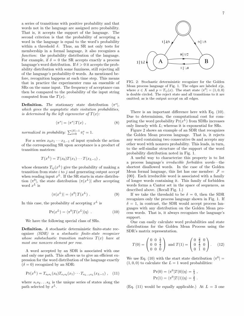
FIG. 2: Stochastic deterministic recognizer for the GoldenMean process language of Fig. 1. The edges are labeled x|p,where x ∈ X and p = Tij(x). The start state 〈π0| = (1, 0, 0)is double circled. The reject state and all transitions to it areomitted; as is the output accept on all edges.

There is an important difference here with Eq. (10).Due to determinism, the computational cost for com-puting the word probability Pr(xL) from SDRs increasesonly linearly with L; whereas it is exponential for SRs.Figure 2 shows an example of an SDR that recognizes

the Golden Mean process language. That is, it rejectsany word containing two consecutive 0s and accepts anyother word with nonzero probability. This leads, in turn,to the self-similar structure of the support of the wordprobability distribution noted in Fig. 1.A useful way to characterize this property is to list

a process language’s irreducible forbidden words—theshortest disallowed words. In the case of the GoldenMean formal language, this list has one member: F ={00}. Each irreducible word is associated with a familyof longer words containing it. This family of forbiddenwords forms a Cantor set in the space of sequences, asdescribed above. (Recall Fig. 1.)If we take the threshold to be δ = 0, then the SDR

recognizes only the process language shown in Fig. 1. Ifδ = 1, in contrast, the SDR would accept process lan-guages with any distribution on the Golden Mean pro-cess words. That is, it always recognizes the language’ssupport.One can easily calculate word probabilities and state

distributions for the Golden Mean Process using theSDR’s matrix representation.

T (0) =

0 0 13

0 0 12

0 0 0

and T (1) =

0 23

00 1

20

0 1 0

. (12)

We use Eq. (10) with the start state distribution 〈π0| =(1, 0, 0) to calculate the L = 1 word probabilities:

Pr(0) = 〈π0|T (0)|η〉 = 13,

Pr(1) = 〈π0|T (1)|η〉 = 23.

(Eq. (11) would be equally applicable.) At L = 3 one

8

finds for x3 = 011:

Pr(011) = 〈π0|T (011)|η〉 = 〈π0|T (0)T (1)T (1)|η〉 = 16.

In fact, all L = 3 words have the same probability, exceptfor x3 = 101, which has a higher probability, Pr(101) =13, and x3 ∈ {000, 001, 100}, for which Pr(x3) = 0. (Cf.

the L = 3 word distribution in Fig. 1.)The conditional probability of a 1 following a 0, say, is

calculated in a similarly straightforward manner:

Pr(1|0) = Pr(01)

Pr(0)=

〈π0|T (0)T (1)|η〉〈π0|T (0)|η〉 = 1 .

Whereas, the probability Pr(0|0) of a 0 following a 0 iszero, as expected.

B. Stochastic Generators

As noted in the introduction, finite-state machines gen-erating strings of symbols can serve as useful models forstructure in dynamical systems. They have been usedas computational models of classical dynamical systemsfor some time; see Refs. [14, 17, 19, 31, 32, 33, 34], forexample.As we also noted, automata that only generate outputs

are less often encountered in formal language theory [29]than automata operating as recognizers. One reason isthat redefining a conventional recognizer to be a devicethat generates output words is incomplete. A mechanismfor choosing which of multiple transitions to take whenleaving a state needs to be specified. And this leads nat-urally to probabilistic transition mechanisms, as one wayof completing a definition. We will develop finite-stategenerators by paralleling the development of SRs.

Definition. A stochastic finite-state generator (SG) isa stochastic transducer with |X | = 1.

The input symbol can be considered a clock signal thatdrives the machine from state to state. The transitionmatrices can be simplified to T (y) = T (y|x). An SG’sstate-to-state transition probabilities are given by thestochastic state-to-state transition matrix :

T =∑

y∈Y

T (y) . (13)

Word probabilities are calculated as with SRs, save thatone exchanges input symbols x with output symbols y:

Pr(yL) = 〈π0|T (yL)|η〉 . (14)

We define the following special class of SGs.

Definition. A stochastic deterministic finite-state gen-erator (SDG) is a stochastic finite-state generator inwhich each matrix T (y) has at most one nonzero entryper row.

As with SDRs, given the generator’s state and an out-put symbol, the next state is uniquely determined. Sim-ilarly, it is less costly to compute word probabilities:

Pr(yL) = Ts0s1(y0)Ts1s2(y1) · · ·TsL−1sL(yL−1) . (15)

Given an initial state distribution, a sum is taken overstates, weighted by their probability. Even so, the com-putation increases only linearly with L. In the followingwe concentrate on SDGs.As an example, consider the generator for the Golden

Mean process language. Its matrix representation isthe same as for the Golden Mean recognizer given inEqs. (12). Its graphical representation is the same asin Fig. 2, except that the edge labels x|p there shouldbe given as p|y. (We return to the relationship betweenrecognizers and equivalent generators shortly.) It turnsout this is the smallest generator, but the proof of thiswill be presented elsewhere.One can easily calculate word probabilities and state

distributions for the Golden Mean Process using theSDG’s matrices. Let us consider a method, different fromthat used above for SRs, that computes probabilities us-ing the asymptotically recurrent states only. This is doneusing the stationary state distribution and the transi-tion matrices restricted to the asymptotically recurrentstates. The method is useful whenever the start stateis not known, but the asymptotic behavior of the ma-chine is. The transition matrices for the SDG, followingEqs. (12), become:

T (0) =

(

0 12

0 0

)

and T (1) =

(

12

01 0

)

. (16)

The stationary state distribution 〈πs| is the left eigen-vector of the state-to-state transition matrix T , Eq. (13):〈πs| = 〈2

3, 13|.

Assuming that the initial state is not known, but theprocess has been running for a long time, we use Eq. (14)with 〈πs| to calculate the L = 1 word probabilities:

Pr(0) = 〈πs|T (0)|η〉 = 13,

Pr(1) = 〈πs|T (1)|η〉 = 23.

At L = 3 one finds for y3 = 011:

Pr(011) = 〈πs|T (011)|η〉 = 〈πs|T (0)T (1)T (1)|η〉 = 16.

All L = 3 words have the same probability, except fory3 = 101, which has a higher probability, Pr(101) = 1

3,

and y3 ∈ {000, 001, 100}, for which Pr(y3) = 0. (Cf. theL = 3 distribution in Fig. 1.)These are the same results found for the Golden Mean

Process recognizer. There, however, we used a differentinitial distribution. The general reason why these twocalculations lead to the same result is not obvious, butan explanation would take us too far afield.As a second example of an SDG consider the Even Pro-

cess whose language consists of blocks of even numbers of

9

FIG. 3: A deterministic generator of the Even Process: Blocksof an even number of 1s are separated by 0s. Only the asymp-totically recurrent states are shown. Edges are labeled p | y,where y ∈ Y and p = Tij(y). The numbers in parenthesesgive a state’s asymptotic probability.

1s bounded by 0s. The substochastic transition matricesfor its recurrent states are

T (0) =

(

12

00 0

)

and T (1) =

(

0 12

1 0

)

. (17)

The corresponding graph is shown in Fig. 3. Noticethat the state-to-state transition matrix T is the same asthe previous model of the Golden Mean Process. How-ever, the Even Process is substantially different; andits SDG representation lets us see how. The set ofirreducible forbidden words is countably infinite [22]:F = {012k+10 : k = 0, 1, 2, . . .}. Recall that theGolden Mean Process had only a single irreducible for-bidden word {00}. One consequence is that the words inthe Even Process have a kind of infinite correlation: the“evenness” of the length of 1-blocks is respected over ar-bitrarily long words. This makes the Even Process effec-tively non-finite: As long as a sequence of 1s is produced,memory of the initial state distribution persists. Anotherdifference is that the support of the word distribution hasa countable infinity of distinct Cantor sets—one for eachirreducible forbidden word. Thus, the Even Process fallsinto the broader class of finitary processes.

C. Properties

We can now describe the similarities and differencesbetween stochastic and other kinds of recognizers andbetween the various classes of generators. Let S(M) de-note the stochastic language recognized or generated byautomaton M. Let P(C) denote the set of stochasticlanguages generated or recognized by machines in classC.The relationships between the languages associated

with the various machine types follow rather directlyfrom their definitions. We swap input and output alpha-bets and reinterpret the same transition matrices, eitheras specifying x|p or p|y as required. All, that is, exceptfor the last two results, which may be unexpected.

Proposition 1. For every SR, supp S(SR) is a regularlanguage.

Proof. The graph of an SR, removing the probabilities,defines a finite-state recognizer and accepts, by definition,

a regular language [29]. This regular language is the sup-port of S(SR) by construction.

Proposition 2. For every SR, S(SR) is a process lan-guage.

Proof. The first property to establish is that the set ofwords recognized by an SR is subword closed: if Pr(xL) >0, then all w ∈ sub(xL) have Pr(w) > 0. This is guar-anteed by definition, since the first input symbol not en-countering an allowed transition leads to rejection of thewhole input, see the SR definition.The second property to establish is that the word dis-

tribution Pr(xL) is normalized at each L. This followsfrom T in Eq. 6 being stochastic.

Proposition 3. SGs and SRs generate and recognize,respectively, the same set of languages: P(SG) = P(SR).

Proof. Consider SG’s transition matrices T (y) and forma new set T (x) in which X = Y . The T (x) define an SRthat recognizes S(SG).It follows that P(SG) ⊆ P(SR).Now consider SR’s transition matrices T (x) and form

a new set T (y) in which Y = X. The T (y) define an SGthat generates S(SR).It follows that P(SG) = P(SR).

Corollary 1. For every SG, supp S(SG) is a regularlanguage.

Corollary 2. For every SG, S(SG) is a process lan-guage.

Corollary 3. SDGs and SDRs generate and recognize,respectively, the same set of languages: P(SDG) =P(SDR).

These equivalences are intuitive and expected. Theydo not, however, hint at the following, which turn on theinterplay between nondeterminism and stochasticity.

Proposition 4. There exists an SG such that P(SG) isnot recognized by any SDR.

Proof. We establish this by example. Consider the non-deterministic generator in Fig. 4, the Simple Nondeter-ministic Source (SNS). To show that there is no possibleconstruction of an SDR we argue as follows. If a 0 ap-pears, then the generator is in state A. Imagine this isthen followed by a block 1k. At each k the generator isin either state A or B. The probability of seeing a 0 nextis ambiguous (either 0 or 1/2) and depends on the exacthistory of internal states visited. Deterministic recogni-tion requires that a recognizer be in a state in which theprobability of the next symbol is uniquely given. Whilereading in 1s the recognizer would need a new state foreach 1 connecting to the same state (state A) on a 0.Since this is true for all k, there is no finite-state SDRthat recognizes the SNS’s process language.

10

FIG. 4: A nondeterministic generator that produces a pro-cess language not recognized by any (finite-state) SDR. Onlyasymptotically recurrent states are shown. Edges are labeledp | y, where y ∈ {0, 1} and p = Tij(y).

Ref. [16] gives an SDR for this process that is minimal,but has a countably infinite number of states. Note thatsupp P(SNS) is the support of the Golden Mean processlanguage.

Corollary 4. There exists an SR such that P(SR) isnot generated by any SDG.

These propositions say, in essence, that deterministicmachines generate or recognize only a subset of the fini-tary process languages. In particular, Props. 3, 4, andCor. 3 imply proper containment: P(SDR) ⊂ P(SG)and P(SDG) ⊂ P(SR). This is in sharp contrast withthe standard result in formal language theory: determin-istic and nondeterministic automata recognize the sameclass of languages—the regular languages [29].This ends our development of classical machines and

their specializations. We move on to their quantumanalogs, following a strategy that is familiar by now.

V. FINITARY QUANTUM PROCESSES

As with stochastic processes, the evolution of a quan-tum system is monitored by a series of measurementoutcomes—numbers registered in some way. Each out-come can be taken to be the realization of a randomvariable. The distribution over sequences of these ran-dom variables is what we call a quantum process. Wewill consider the finitary version of quantum processes inthe same sense as used for the classical stochastic pro-cesses: The internal resources used during the evolutionare finitely specified.

A. Quantum States

Quantum mechanics is sometimes viewed as a general-ization of classical probability theory with noncommut-ing probabilities. It is helpful, therefore, to compare clas-sical stochastic automata and quantum automata and, inparticular, to contrast the corresponding notions of state.The goal is to appreciate what is novel in quantum au-tomata. The reader should have a working knowledge ofquantum mechanics at the level of, say, Ref. [35].In the classical (stochastic) setting an automaton has

internal states S and also a distribution 〈π| over them.

The distribution itself can be taken to be a “state”,but of what? One interpretation comes from consider-ing how an observer monitors a series of outputs froma stochastic generator and predicts, with each observedsymbol, the internal state s ∈ S the automaton is in.This prediction is a distribution 〈π| over the internalstates—one that represents the observer’s best guess ofthe automaton’s current internal state. In this sensethe distribution is the state of the best predictor. If〈π| = (0, . . . , 0, πi = 1, 0, . . . , 0), then the observer knowsexactly what internal state, si ∈ S, the automaton is in.For these special cases one can identify state distributionsand internal states.

Similarly, there are several kinds of state that onemight define for a quantum automaton. Each quantumautomaton will consist of internal states and we will takethe state of the automaton to be a superposition overthem. The central difference with classical (stochastic)automata is that the superposition over internal statesis not a probability distribution. In particular, inter-nal states have complex amplitudes and, therefore, theypotentially interfere. This, in turn, affects the processlanguage associated with the quantum automaton.

In contrast with quantum automata, the state of aquantum dynamical system depends on the choice of abasis that spans its state space. The state is completelyspecified by the system’s state vector, a unit vector repre-sented as a sum of basis states that span the state space.However, if one chooses a basis consisting of the eigen-states of an observable and associates them with internalstates of quantum automaton, there is a simple corre-spondence between a state vector of a quantum dynam-ical system (a superposition of basis states) and a stateof a quantum automaton (a superposition over internalstates). Thus, we will use the terms internal states (ofan automaton) and basis states (of a quantum dynam-ical system’s state space) interchangeably. By similarreasoning, the state vector (of a quantum dynamical sys-tem) and state (of a quantum automaton) will be usedinterchangeably.

In the vocabulary of quantum mechanics, at any mo-ment in time a given quantum automaton is in a purestate—another label for a superposition over internalstates. An observer’s best guess as to the automaton’scurrent pure state is a probability distribution over statevectors—the so-called mixed state.

It is helpful to imagine a collection of individual quan-tum automata, each in a (pure) state, that is specified bya distribution of weights. One can also imagine a singlequantum automaton being in different pure states at dif-ferent moments in time. The time-averaged state then isalso a mixed state. It is the latter picture that we adopthere.

The fact that a quantum pure state can be a super-position of basis states is regarded as the extra structureof quantum mechanics that classical mechanics does nothave. We respect this distinction by building a hierarchyof quantum states that goes from basis states to superpo-

11

sitions of basis states to mixtures of superpositions. Theanalogous classical-machine hierarchy goes only from in-ternal states to distributions over internal states.

B. Quantum Measurement

We now turn to the measurement process, a crucial andalso distinctive component in the evolution of a quantumdynamical system, and draw parallels with quantum au-tomata. In setting up an experiment, one makes choicesof how and when to measure the state of a quantum sys-tem. These choices typically affect what one observes,and in ways that differ radically from classical dynami-cal systems.

Measurement is the experimental means of character-izing a system in the sense that the observed symbolsdetermine the process language and any subsequent pre-diction of the system’s behavior. The measurement of aquantum mechanical system is described by a Hermitianoperator that projects the current state onto one (or sev-eral) of the operator’s eigenstates. After a measurement,the system is, with certainty, in the associated (subset of)eigenstate(s). Such an operator is also called an observ-able and the eigenvalues corresponding to the eigenstatesare the observed measurement outcomes.

To model this situation with a quantum automaton,we identify the states of the automaton with the eigen-states of a particular observable. A measurement is de-fined through an operator that projects the automaton’scurrent state vector onto one (or a subset) of its internal(basis) states. The “observed” measurement outcome isemitted as a symbol labeling the transition(s) which enterthat internal state (or that subset of states).

VI. QUANTUM TRANSDUCERS

The study of quantum finite-state automata has pro-duced a veritable zoo of alternative models for languagerecognition. (These are reviewed below in Section VIIB.)Since we are interested in recognition, generation, andtransduction of process languages, we start out defininga generalized quantum-finite state transducer and thenspecialize. We develop a series of quantum finite-state au-tomaton models that are useful for recognition and gener-ation and, ultimately, for modeling intrinsic computationin finitary quantum processes. It is worth recalling thatthese quantum finite-state machines form the lowest levelof a hierarchy of quantum computational models. Thus,they are less powerful than quantum Turing machines.Nevertheless, as we will see, they exhibit a diversity ofinteresting behaviors. And, in any case, they representcurrently feasible quantum computers.

A. Definition

We define a quantum transducer that corresponds tothe standard quantum mechanical description of a phys-ical experiment.

Definition. A quantum transducer (QT) is a tuple{Q, 〈ψ| ∈ H, X, Y,T(Y |X)} where

1. Q = {qi : i = 0, . . . , n − 1} is a set of n internalstates.

2. The state vector 〈ψ| lies in an n-dimensionalHilbert space H; its initial value is the start state〈ψ0|.

3. X and Y are finite alphabets for input and outputsymbols, respectively.

4. T(Y |X) is a set of n × n transition matrices{T (y|x) = U(x)P (y), x ∈ X, y ∈ Y } that are prod-ucts of

(a) a unitary matrix U(x): U †(x) = U−1(x) (†denotes complex transpose); and

(b) a projection operator P (y).

At each time step a quantum transducer (QT ) reads asymbol x ∈ X from the input, outputs a symbol y ∈ Y ,and updates its state vector 〈ψ| via T (y|x).

The preceding discussion of state leads to the followingcorrespondence between a QT’s internal states and statevectors.

Definition. One associates an internal state qi ∈ Q withthe eigenstate 〈φi| of an observable such that:

1. For each qi ∈ Q there is a basis vector 〈φi| =(0, . . . , 1, . . . , 0) with a 1 in the ith component.

2. The set {〈φi| : i = 0, 1, . . . , n− 1} spans the Hilbertspace H.

Definition. A state vector 〈ψ| ∈ H is a unit vector. Itcan be expanded in terms of basis states 〈φi|:

〈ψ| =n−1∑

i=0

〈φi| ci , (18)

with ci ∈ C and∑n−1

i=0 c∗i ci = 1.

Identifying internal states qi and basis states 〈φi| con-nects the machine view of a quantum dynamical systemwith that familiar from standard developments of quan-tum mechanics. A QT state is given by its current statevector 〈ψ|. At each time step a symbol x is read in, whichselects a unitary operator U(x). The operator is appliedto the state vector and the result is measured via P (y).The output, an eigenvalue of the observable, is symbol y.We describe a QT’s operation via the evolution of a

bra (row) vector. We make this notational choice, which

12

is unconventional in quantum mechanics, for two rea-sons that facilitate comparing classical and quantum au-tomata. First, the state distribution of a classical finite-state machine is given conventionally by a row vector.And second, the graphical meaning of a transition fromstate i to j is reflected in the transition matrix entriesTij , only if one uses row vectors and left multiplicationwith T . This is also convention for stochastic processes.

B. Measurement

The projection operators are familiar from quantummechanics and can be defined in terms of the internal(basis) states as follows.

Definition. A projection operator P (y) is the linear op-erator

P (y) = |φi〉 〈φi| , (19)

where φi is the eigenvector of the observable with eigen-value y. In the case of degeneracy P (y) sums over acomplete set {i} of mutually orthogonal eigenstates:

P (y) =∑

{i}|φi〉 〈φi| . (20)

Each P is Hermitian (P † = P ) and idempotent (P 2 =P ).

P ≡ {P (y) : y ∈ Y ∪ {λ}} is the set of projectionoperators with

∑

y∈Y P (y) = 1, where 1 is the identitymatrix. λ is the null symbol and a placeholder for “nomeasurement”. We take P (λ) = 1 and do not include itin the calculation of word probabilities, for example. “Nomeasurement” differs from a non-selective measurementwhere a projection takes place, but the outcome is not de-tected. The decision whether to perform a measurementor not is considered an input to the QT.In the eigenbasis of a particular observable the cor-

responding matrices only have 0 and 1 entries. In thefollowing we assume such a basis. In addition, we con-sider only projective measurements which apply to closedquantum systems. (Open systems will be considered else-where.)In quantum mechanics, one distinguishes between

degenerate and non-degenerate measurement operators[36]. A non-degenerate measurement operator projectsonto one-dimensional subspaces of H. That is, the eigen-vectors of the operator all have distinct eigenvalues. Incontrast, the operators associated with a degenerate mea-surement have degenerate eigenvalues. Such an operatorprojects onto higher-dimensional subspaces of H. Aftersuch a measurement the QT is potentially in a super-position of states

∑

i ci 〈φi|, where i sums over the de-generate set of mutually orthogonal eigenstates. Just asdegeneracy leads to interesting consequences in quantumphysics, we will see in the examples to follow that degen-erate eigenvalues lead to interesting quantum languages.

QTs model a general experiment on a quantum dy-namical system. As such they should be contrasted withthe sequential machines and transducers of Refs. [37] and[38], respectively, that map the current quantum stateonto an output. This mapping, however, is not associ-ated with a measurement interaction and lacks physicalinterpretation.

C. Evolution and Word Distributions

We can now describe a QT’s operation as it scans itsinput. Starting in state 〈ψ0| it reads in a symbol x ∈ Xfrom an input word and updates its state by applying theunitary matrix U(x). Then the state vector is projectedwith P (y) and renormalized. Finally, symbol y ∈ Y isemitted. That is, the state vector after a single time-stepof a QT is given by:

〈ψ(y|x)| = 〈ψ0|T (y|x)√

〈ψ0|T (y|x)T †(y|x)|ψ0〉

=〈ψ0|U(x)P (y)

√

〈ψ0|U(x)P (y)U †(x)|ψ0〉. (21)

In the following we drop the renormalization factor in thedenominator to enhance readability. It will be mentionedexplicitly when a state is not to be normalized.When a QT reads in a length-L word xL ∈ XL and

outputs a length-L word yL ∈ Y L, the transition matrixbecomes

T (yL|xL) = U(x0)P (y0) · · ·U(xL−1)P (yL−1) (22)

and the updated state vector is

〈ψ(yL|xL)| = 〈ψ0|T (yL|xL) . (23)

Starting the QT in 〈ψ0| the conditional probabilityPr(y|x) of the output symbol y given the input symbolx is calculated from the state vector in Eq. (21), beforerenormalization:

Pr(y|x) = 〈ψ(y|x)|ψ(y|x)〉 . (24)

The probability Pr(yL|xL) of output sequence yL condi-tioned on input sequence xL is calculated similarly usingEq. (23):

Pr(yL|xL) = 〈ψ(yL|xL)|ψ(yL|xL)〉 . (25)

D. Properties

We draw out several properties of QTs on our way tounderstanding their behavior and limitations.

Proposition 5. A QT’s output alphabet size is bounded:|Y | ≤ dim(H).

13

Proof. This follows from the QT definition since out-put symbols are directly associated with eigenvalues. Thenumber of eigenvalues is bounded by the dimension of theHilbert space.

Many properties of QTs are related to a subclass ofSTs, those with doubly stochastic transition matrices.Given this, it is useful to recall the relationship betweenunitary and doubly stochastic matrices.

Definition. Given a unitary matrix U , matrix M withMij = |Uij |2 is called a unistochastic matrix.

A unistochastic matrix is doubly stochastic, whichfollows from the properties of unitary matrices. Com-pared to a stochastic transducer, a QT’s structure isconstrained through unitarity and this is reflected in itsarchitecture. A path exists between node i and node jwhen Mij > 0. An equivalent description of a quantumtransducer is given by its graphical representation.Recalling the types of graph state defined in Sec. III B,

we find that only a subset occur in QTs. Specifically, aQT has no transient states.

Proposition 6. Every node i of G(QT), if connected toa set of nodes j 6= i, is a member of a strongly connectedset.

Proof. Given that one path exists from (say) i to j, wemust show that the reverse one exists, going from j toi. According to the definition of a path it is sufficientto show this for the unistochastic matrix Mij = |Uij |2.A doubly stochastic matrix can always be expressed as alinear combination of permutation matrices. Thus, anyvector (0, 0, . . . , 1, . . . ) with only one 1 entry can be per-muted into any other vector with only one 1 entry. Thisis equivalent to saying that, if there is a path from nodei to j there is a path from j to i.

The graph properties of a unitary matrix mentionedhere should be compared with those discussed by Sev-erini [39] and others. The graph of a finite-state machinespecified by a unitary matrix is a directed graph, or di-graph. A digraph vertex is a source (sink) if it has noingoing (no outgoing) arcs. A digraph vertex is isolatedif it is not joined to another. Ref. [39] characterizes thesemachines by assuming their digraphs have no isolatednodes, no sinks, and no sources. Given the precedingproposition the nonexistence of sinks or sources followssimply from assuming no isolated nodes.One concludes that QT graphs are a limited subset of

digraphs, namely the strongly connected ones. Further-more, there is a constraint on incoming edges to a node.

Proposition 7. All incoming transitions to an internalstate are labeled with the same output symbol.

Proof. Incoming transitions to internal state qi are la-beled with output symbol y if 〈φi| has eigenvalue y. Everyeigenstate has a unique eigenvalue, and so the incomingtransitions to any particular state qi are labeled with thesame output symbol representing one eigenvalue.

Proposition 8. A QT’s transition matrices T (y|x)uniquely determine the unitary matrices U(x) and theprojection operators P (y).

Proof. Summing the T (y|x) over all y for each x yieldsthe unitary matrices U(x):

∑

y∈Y

T (y|x) =∑

y∈Y

U(x)P (y) = U(x) . (26)

The P (y) are obtained, from any of the U(x), throughthe inverse of U−1(x) = U †(x):

P (y) = U †(x)T (y|x) . (27)

Definition. A QT is reversible if the automaton definedby the transpose of each U(x) and P (y) is also a QT.

Proposition 9. QTs are reversible.

Proof. The transpose of a unitary matrix is unitary.The transpose of a projection operator is the operator it-self.

Graphically, the reversed QT is obtained by simplyswitching the direction of the edges. This produces atransducer with the transition amplitudes Tji, formerlyTij . The original input and output symbols, whichlabeled ingoing edges to state qi, remain unchanged.Therefore, in general, the languages generated by a QTand its reverse are not the same. By way of contrast,this simple operation applied to an ST does not, in gen-eral, yield another ST. A simple way to summarize theseproperties is that a QT forms a group, an ST forms asemi-group.

VII. QUANTUM RECOGNIZERS AND

GENERATORS

The quantum transducer is our most general construct,describing a quantum dynamical process in terms of in-puts and outputs. We will now specialize quantum trans-ducers into recognizers and generators. We do this byparalleling the strategy adopted for developing classes ofstochastic transducers. For each machine class we firstgive a general definition and then specialize, for example,yielding deterministic variants. We establish a number ofproperties for each type and then compare their descrip-tive powers in terms of the process languages each classcan recognize or generate. The results are collected to-gether in a computational hierarchy of finitary stochasticand quantum processes.

A. Quantum Recognizers

Quantum finite-state machines are almost exclusivelydiscussed as recognizing devices. Following our develop-ment of a consistent set of quantum finite-state trans-ducers, we can now introduce quantum finite-state rec-ognizers as restrictions of QTs and compare these with

14

alternative models of quantum recognizers. Since we areinterested in the recognition of process languages our def-inition of quantum recognizers differs from those intro-duced elsewhere; see Sec. VII B below. The main differ-ence is the recognition of a process language includingits word distribution. The restrictions that will be im-posed on a QT to achieve this are similar to those of thestochastic recognizer.

Definition. A quantum finite-state recognizer (QR) is aquantum transducer with |Y | = 1 and T (y|x) = UP (x) ≡T (x).

One can think of the output symbol y as accept. Thecondition for accepting a symbol is, then,

Pr(x) = 〈ψ0|T (x)T †(x)|ψ0〉 . (28)

If no symbol is output the recognizer has halted andrejected the input. Operationally, recognition works asit does in the classical setting. An experimenter runs anensemble of QRs on the same input. The frequency ofacceptance can then be compared to the probability ofthe input string computed using the T (x).

Definition. A QR accepts a process language P withword-probability threshold δ, if and only if for all w ∈ P

∣

∣Pr(w)−〈ψ0|T (w)T †(w)|ψ0〉∣

∣ ≤ δ (29)

and for all w /∈ P, 〈ψ0|T (w)T †(w)|ψ0〉 = 0.

Acceptance or rejection happens at each time step.We also have deterministic versions of QRs.

Definition. A quantum deterministic finite-state recog-nizer (QDR) is a quantum recognizer with transition ma-trices T (x) that have at most one nonzero element perrow.

B. Alternatives

Quantum finite automata were introduced by severalauthors in different ways, and they recognize differentclasses of languages. To our knowledge the first men-tion of quantum automata was made by Albert in 1983[40]. Albert’s results have been subsequently criticizedby Peres as being based on an inadequate notion of mea-surement [41].Kondacs and Watrous introduced 1-way and 2-way

quantum finite-state automata [42]. The 1-way automataread symbols once and from left to right (say) in the inputword. Their 2-way automata scan the input word manytimes moving either left to right or right to left. The au-tomata allow for measurements at every time step, check-ing for acceptance, rejection, or continuation. They showthat a 2-way QFA can recognize all regular languages andsome nonregular languages. 1-way QFA are less power-ful: They can only recognize a subset of the regular lan-guages. A more powerful generalization of a 1-way QFA

is a 1-way QFA that allows mixed states, introduced byAharonov et al [43]. They also allow for nonunitary evo-lution. Introducing the concept of mixed states simplyadds classical probabilities to quantum probabilities andis inherent in our model of QTs.The distinctions between these results and the QRs in-

troduced here largely follow from the difference betweenregular languages and process languages. Thus, the re-sult in Ref. [42] that no 1-way quantum automaton canrecognize the language (0+1)∗0, does not apply to QTs.It clearly is a regular language, but not a process lan-guage. Also, the result by Bertoni and Carpentieri thatquantum automata can recognize nonregular languages,does not apply here [44]. They find that a quantum au-tomaton that is measured only after the whole input hasbeen read in can recognize a nonregular language. A QR,however, applies measurement operators for every sym-bol that is being read in.Moore and one of the authors introduced 1-way quan-

tum automata (without using the term “1-way”) [45]. Itis less powerful than the 1-way automata of Kondacs andWatrous, since it allows only for a single measurement af-ter the input has been read in. They also introduced ageneralized quantum finite-state automaton whose tran-sition matrices need not be unitary, in which case allregular languages are recognized. A type of quantumtransducer mentioned earlier, a quantum sequential ma-chine was introduced by Gudder [37]. The link, however,between machine output and quantum physical measure-ment is missing. Freivalds and Winter introduced quan-tum transducers [38] that at each step perform a mea-surement to determine acceptance, rejection, or contin-uation of the computation. In addition, they map thecurrent quantum state onto an output. Here too, themapping is not associated with a measurement interac-tion and lacks physical interpretation.These alternative models for quantum automata ap-

pear to be the most widely discussed. There are others,however, and so the above list is by no means complete.Our motivation to add yet another model of quantumfinite-state transducer and recognizer to this list is theinability of the alternatives to recognize or process lan-guages that represent quantum dynamical systems sub-ject to repeated measurement.

C. Quantum Generators

We now introduce quantum finite-state generators asrestrictions of QTs and as a complement to recogniz-ers. They serve as a representation for the behavior ofautonomous quantum dynamical systems. In contrastto quantum finite-state recognizers, quantum finite-stategenerators appear to not have been discussed before. Aquantum generator is a QT with only one input. As inthe classical case, one can think of the input as a clocksignal that drives the machine through its transitions.

15

Definition. A quantum finite-state generator (QG) is aquantum transducer with |X | = 1.

At each step it makes a transition from one state toanother and emits a symbol. As in the classical casethere are nondeterministic (just implicitly defined) anddeterministic QGs.

Definition. A quantum deterministic finite-state gener-ator (QDG) is a quantum generator in which each matrixT (y) has at most one nonzero entry per row.

Interestingly, there is a mapping from a given QDG toa classical automaton.

Definition. Given a QDG M = {U, P (y)}, the equiv-alent (classical) SDG M′ = {T (y)} has unistochas-tic state-to-state transition matrix T with componentsTij = [Uij ]

2.

We leave the technical interpretation of “equivalent”to Thm. 2 below.As mentioned earlier, in quantum mechanics one dis-

tinguishes between degenerate and non-degenerate mea-surements. Having introduced the different types ofquantum generators, we can now make a connection todegenerate measurements.

Definition. A quantum complete finite-state genera-tor (QCG) is a quantum generator observed via non-degenerate measurements.

In order to average over observations, we must extendthe formalism of quantum automata to describe distri-butions over state vectors. Recalling the notions of statediscussed in Section VA, this means we need to describemixed states and their evolution.Let a system be described by a state vector 〈ψi| at time

t. If we do not know the exact form of 〈ψi| but only aset of possible 〈ψi| , i = 0, ..., k−1, then we give the bestguess as to the system’s state in terms of a statistical mix-ture of the 〈ψi|. This statistical mixture is representedby a density operator ρ with weights pi assigned to the〈ψi|:

ρ =

k−1∑

i=0

pi |ψi〉 〈ψi| . (30)

The main difference from common usage of “mixed state”is that we compare the same state over time; whereas,typically different systems are compared at a single time.Nevertheless, in both cases, the density matrix formalismapplies.

D. Properties

With this notation in hand, we can now establish anumber of properties of quantum machines.

Definition. A QG’s stationary state ρs is the mixedstate that is invariant under unitary evolution and mea-surement:

ρs =∑

y∈Y

P (y)U †ρsUP (y) . (31)

ρs is the mixed state which the quantum machine is inon average, since we are describing a single system that isalways in a pure state. The stationary state is thereforethe best guess of an observer ignorant of the machine’sstate.

Theorem 1. A QG’s stationary state is the maximallymixed state:

ρs = n−1

n−1∑

i=0

|φi〉 〈φi| = 1/n . (32)

Proof. Since the 〈φi| are basis states, ρs is a diagonalmatrix equal to the identity multiplied by a factor. Re-call that the stationary distribution of a Markov chainwith doubly stochastic transition matrix is always uni-form [46]. And so, we have to establish that ρs is aninvariant distribution:

ρs =∑

y∈Y

P (y)U †ρsUP (y) (33)

= n−1∑

y∈Y

P (y)U †UP (y) (34)

= n−1∑

y∈Y

P (y) = 1/n . (35)

Now we can calculate the asymptotic symbol probabil-ities, using the density matrix formalism for computingprobabilities of measurement outcomes [47], and ρs.

Proposition 10. A QG’s symbol distribution dependsonly on the dimensions of the projection operators andthe Hilbert space.

Proof. Denote the trace operator by tr, then we have

Pr(y) = tr(

T †(y)ρsT (y))

= n−1tr(

T †(y)1T (y))

= n−1tr(

P †(y)U †UP (y))

= n−1tr(

P †(y)1P (y))

= n−1tr (P (y))

= n−1dim P (y) . (36)

Although the single-symbol distribution is determinedby the dimension of the subspaces onto which the P (y)project, distributions of words yL with L > 1 are notsimilarly restricted. The asymptotic word probabilitiesPr(yL) are:

Pr(yL) = tr(

T †(yL)ρsT (yL))

. (37)

No further simplification is possible for the general case.Analogous results follow for QRs, except that the cal-

culations are suitably modified to use T (x).

16

E. Finitary Process Hierarchy

To better appreciate what these machines are capa-ble of we amortize the effort in developing the preced-ing results to describe the similarities and differences be-tween quantum recognizers and generators, as well asbetween stochastic and quantum automata. We collectthe results, give a summary and some interpretation, andpresent a road map (Fig. 5) that lays out the computa-tional hierarchy of finitary quantum processes. As above,S(M) denotes the stochastic language associated withmachine or machine typeM and P(C), the set of stochas-tic languages generated or recognized by all machines inclass C.

Proposition 11. QCGs are deterministic.

Proof. Since all projection operators have dimensionone, all transition matrices have at most one nonzeroelement per row. This is the condition for being a QDG.

Non-degenerate measurements always define a QDG.There are degenerate measurements, however, that alsocan lead to QDGs, as we will show shortly. One concludesthat P(QCG) ⊂ P(QDG).We now show that for any QDG there is an SDG gener-

ating the same stochastic language. Thereby we establishobservational equivalence between the different classes ofmachine.

Theorem 2. Every S(QDG) is generated by some SDG:P(QDG) ⊆ P(SDG).

Proof. We show that the SDG generating S(QDG) is theequivalent SDG, as defined in Sec. VIIC, and that theQDG M and its equivalent SDG M′ generate the sameword distribution and so the same stochastic language.The word probabilities PrM(yL) for M are calculated

using Eq. (37) and the QDG’s transition matrices TM′ :

PrM(yL) = tr(

T †M(yL)ρsTM(yL)

)

= n−1tr(T †T )

= n−1∑

i

[T †T ]ii

= n−1∑

i

∑

j

T †ijTji

= n−1∑

ij

T 2ij .

The word probabilities PrM ′(yL) for M ′ are calculatedusing Eq. (14) and the SDG’s transition matrices TM:

PrM′(yL) = 〈π0|TM′(yL)|η〉

=

n−1∑

i=0

π0i

∑

j

(TM′(yL))ij

= n−1

n−1∑

i,j=0

(TM′(yL))ij . (38)

Since (TM(yL))2ij = (TM′(yL))ij , from the definition ofan equivalent SDG, the claim follows.

More than one QDG can be observationally equivalentto a given SDG. The reason for this to occur is that thequantum mechanical phases of the transition amplitudescancel in the transformation from a QDG.We can now easily characterize languages produced by

QDGs.

Corollary 5. For every QDG, supp S(QDG) is a reg-ular language.

Proof. This follows directly from Thm. 2 and Cor. 1.

Corollary 6. For every QDG, S(QDG) is a process lan-guage.

Proof. This follows directly from Thm. 2 and Cor. 2.

With this we can begin to compare the descriptivepower of the different machine types.

Proposition 12. QGs and QRs are equivalent: Theyrecognize and generate the same set of stochastic lan-guages, respectively: P(QG) = P(QR).

Proof. Consider QG’s transition matrices T (y) =UP (y) and form a new set T (x) = UP (x) in whichP (x) = P (y), associating the QR’s input X with theQG’s output Y . The T (x) define a QR that recognizesS(QG). It follows that P(QG) ⊆ P(QR).Now consider QR’s transition matrices T (x) = UP (x)

and form a new set T (y) in which P (y) = P (x), asso-ciating inputs and outputs as above. The T (y) define aQG that generates S(QR).It follows that P(QG) = P(QR).

Corollary 7. QDGs and QDRs are equivalent: Theyrecognize and generate the same set of stochastic lan-guages, respectively: P(QDG) = P(QDR).

Proof. Prop. 12’s proof goes through if one restricts todeterministic machines.

Corollary 8. For every QDR, supp S(QDR) is a reg-ular language.

Proof. This follows directly from Cor. 1 and Cor. 7.

Corollary 9. For every QDR, S(QDR) is a process lan-guage.

Proof. This follows directly from Cor. 6 and Cor. 7.

Proposition 13. There exists an SDG such thatP(SDG) is not generated by any QDG.

Proof. The process language generated by the SDG given

by T (0) =(

1√2

)

and T (1) =(

1− 1√2

)

(a biased

coin) cannot be generated by any QDG. According toProp. 10 Pr(y) = n−1dimP (y), which is a rational num-ber, whereas Pr(y) for the above biased coin is irrational.

17

FIG. 5: Finitary process language hierarchy: Each circle rep-resents the set of process languages recognized or generatedby the inscribed machine class. Increasing height indicatesproper containment; machine classes at the same height arenot directly comparable. The hierarchy summarizes the the-orems, propositions, and corollaries in Secs. IVC and VIIE.

Corollary 10. P(QDG) ⊂ P(SDG).

Proof. From Thm. 2 and Prop. 13.

Corollary 11. P(QDR) ⊂ P(SDR):

Proof. From Cor. 3, Cor. 7, Thm. 2, and Prop. 13.

At this point it is instructive to graphically summarizethe relations between recognizer and generator classes.Figure 5 shows a machine hierarchy in terms of sets oflanguages recognized or generated. The class of QCGs isat the lowest level. This is contained in the class of QDGsand QDRs. The languages they generate or recognizeare properly included in the set of languages generatedor recognized by classical deterministic machines—SDGsand SDRs. These, in turn, are included in the set oflanguages recognized or generated by classical nondeter-ministic machines, SGs and SRs, as well as QRs andQGs.

The preceding results serve to indicate how portionsof the finitary process hierarchy are organized. However,there is still more to understand. For example, the reg-ularity of the support of finitary process languages, thehierarchy’s dependence on acceptance threshold δ, andthe comparability of stochastic and quantum nondeter-ministic machines await further investigation.

VIII. QUANTUM GENERATORS AND

FINITARY PROCESSES: EXAMPLES

To appreciate what can be done with quantum ma-chines, we will illustrate various features of QTs by mod-eling several prototype quantum dynamical systems. Westart out with deterministic QGs, building one to modela physical system, and end on an example that illustratesa nondeterministic QT.

A. Two-State Quantum Processes

According to Prop. 10 the symbol distribution gener-ated by a QG only depends on the dimension of the pro-jection operator and the dimension of the Hilbert space.What are the consequences for two-state QGs? First ofall, according to Cor. 5 the maximum alphabet size is 2.The corresponding projection operators can either havedimension 2 (for a single-letter alphabet) or dimension1 for a binary alphabet. The only symbol probabilitiespossible are Pr(y) = 1 for the single-letter alphabet andPr(y) = 1/2 for a binary alphabet. So one can set asidethe single-letter alphabet case as too simple.We also see that a binary-alphabet two-state QDG can

produce only a highly restricted set of process languages.It is illustrative to look at the possible equivalent SDGs.Their state-to-state transition matrices are given by

T =

(

p 1− p1− p p

)

, (39)

with p ∈ {0, 1/2, 1}.For p = 1/2, for example, this is the fair coin process.

It becomes immediately clear that the Golden Mean andthe Even processes, which are modeled by two-state clas-sical automata, cannot be represented with a two-stateQDG. (The three-state models are given below.)

1. Iterated Beam Splitter

Let’s consider a physical two-state process and build aquantum generator for it.The iterated beam splitter is an example that, despite

its simplicity, makes a close connection with real experi-ment. Figure 6 shows the experimental apparatus. Pho-tons are sent through a beam splitter (thick dashed line),producing two possible paths. The paths are redirectedby mirrors (thick horizontal solid lines) and recombinedat a second beam-splitter. From this point on the sameapparatus is repeated indefinitely to the right. After thesecond beam-splitter there is a third and a fourth andso on. Single-photon quantum nondemolition detectorsare located along the paths, between every pair of beam-splitters. One measures if the photon travels in the upperpath and the other determines if the photon follows thelower path.This is a quantum dynamical system: a photon passing

repeatedly through various beam splitters. It has a two-dimensional state space with two eigenstates—“above”and “below”. Its behavior is given by the evolution of astate vector 〈ψ|. The overall process can be representedin terms of a unitary operation for the beam splitter andprojection operators for the detectors. The unitary op-erator for the beam splitter is the Hadamard matrix UH :

UH =1√2

(

1 11 −1

)

. (40)

18

FIG. 6: Experimental set-ups for the iterated beam splitter:Solid lines are mirrors; beam splitters, horizontal dashed lines.Photon nondemolition detectors, marked as D, are placed be-tween every pair of beam splitters. Under measurement pro-tocol I all detectors are in operation; under protocol II onlythe solid-line detectors are activated. The apparatus is re-peated indefinitely to the right.

The measurement operators have the following matrixrepresentation in the experiment’s eigenbasis:

P (0) =

(

1 00 0

)

and P (1) =

(

0 00 1

)

, (41)

where the measurement symbol 0 stands for “above” andsymbol 1 stands for “below”.Before we turn to constructing a quantum finite-state

generator to model this experiment we can understandintuitively the sequence of outcomes that results fromrunning the experiment for long times. If entering thebeam splitter from above, the detectors record the pho-ton in the upper or lower path with equal probability.Once the photon is measured, though, it is in that de-tector’s path with probability 1. And so it enters thebeam splitter again via only one of the two possiblepaths. Thus, the second measurement outcome will havethe same uncertainty as the first: the detectors report“above” or “below” with equal probability. The resultingsequence of outcomes after many beam splitter passagesis simply a random sequence. Call this measurement pro-tocol I.Now consider altering the experiment slightly by re-

moving the detectors after every other beam splitter. Inthis configuration, call it protocol II, the photon entersthe first beam splitter, does not pass a detector and in-terferes with itself at the next beam splitter. That inter-ference, as we will confirm shortly, leads to destructiveinterference of one path after the beam splitter. The pho-ton is thus in the same path after the second beam split-ter as it was before the first beam splitter. A detectorplaced after the second beam splitter therefore reportswith probability 1 that the photon is in the upper path,if the photon was initially in the upper path. If it wasinitially in the lower path, then the detector reports thatit is in the upper path with probability 0. The resultingsequence of upper-path detections is a very predictablesequence, compared to the random sequence from proto-col I.We now construct a QG for the iterated-beam splitter

using the matrices of Eqs. (40)-(41) and the stationarystate of Eq. (32). The output alphabet consists of twosymbols denoting detection “above” or “below”: Y ={0, 1}. The set of states consists of the two eigenstatesof the system “above” and “below”: Q = {A,B}. Thetransition matrices are:

T (0) = UHP (0) =1√2

(

1 01 0

)

, (42a)

T (1) = UHP (1) =1√2

(

0 10 −1

)

. (42b)

The resulting QG turns out to be deterministic, as can beseen from its graphical representation, shown in Fig. 7.The word distribution for the process languages gen-

erated by protocols I and II are obtained from Eq. (37).Word probabilities for protocol I (measurement at eachtime step) are, to give some examples:

Pr(0) = n−1dim(P (0)) =1

2, (43a)

Pr(1) = n−1dim(P (1)) =1

2, (43b)

Pr(00) = tr(

T †(0)T †(0)ρsT (0)T (0))

=1

4, (43c)

Pr(01) = Pr(10) = Pr(11) =1

4. (43d)

Continuing the calculation for longer words shows thatthe word distribution is uniform at all lengths Pr(yL) =2−L.For protocol II (measurement every other time step)

we find:

Pr(0) = tr(

T †(λ0)ρsT (λ0))

=1

2, (44a)

Pr(1) = tr(

T †(λ1)ρsT (λ1))

=1

2, (44b)

Pr(00) = tr(

T †(λ0λ0)ρsT (λ0λ0))

=1

2, (44c)

Pr(11) = tr(

T †(λ1λ1)ρsT (λ1λ1))

=1

2, (44d)

Pr(10) = Pr(01) = 0 . (44e)

If we explicitly denote the output at the unmeasured timestep as λ, the sequence 11 turns into λ1λ1, as do theother sequences in protocol II. As one can see, the wordprobabilities calculated from the QDG agree with ourearlier intuitive conclusions.Comparing the iterated beam splitter QDG to its clas-

sically equivalent SDG reveals several crucial differencesin performance. Following the recipe from Sec. VII E, onhow to build an SDG from a QDG, gives the classicalgenerator shown in Fig. 8(a). Its transition matrices are:

T (0) =1

2

(

1 01 0

)

and T (1) =1

2

(

0 10 1

)

. (45)

The symbol sequence generated by this SDG for proto-col I is the uniform distribution for all lengths, as can be

19

FIG. 7: Quantum finite-state machine for the iterated beamsplitter: The resulting symbol sequences are statistically iden-tical to the sequences obtained with the measurement proto-cols I and II shown in Fig. 6. When no measurement is made,transitions along all edges occur.

FIG. 8: Classical deterministic generators for the iteratedbeam splitter: (a) Protocol I and (b) protocol II, p = 2. (Cf.Fig. 6.)

easily verified using Eq. (14) or, since it is deterministic,Eq. (15). This is equivalent to the language generatedby the QDG under protocol I. However, the probabilitydistribution of the sequences for the generator under pro-tocol II, ignoring every second output symbol, is still theuniform distribution for all lengths L. This could not bemore different from the language generated by the QDGunder protocol II.The reason is that the classical machine is unable to

capture the interference effects present in experimentalprotocol II. A second SDG has to be constructed from theQDG’s transition matrices for set-up II. This is done bycarrying out the matrix product first and then formingits equivalent SDG. The result is shown Fig. 8(b). Itstransition matrices are:

T (0) =1

2

(

1 00 0

)

and T (1) =1

2

(

0 00 1

)

. (46)

The two classical SDGs are clearly (and necessarily)different. Thus, a single QG can model a quantumsystem’s dynamics for different measurement protocols.Whereas an SG only captures the behavior of each indi-vidual experimental set-up. This simple example servesto illustrate the utility of QGs over SGs in modeling thebehavior of quantum dynamical systems.

B. Three-State Quantum Processes

1. Golden Mean Quantum Machine

Recall the classical Golden Mean generator ofSec. IVB. A QDG, which generates the same processlanguage, is shown in Fig. 9. Consider a spin-1 particlesubject to a magnetic field that rotates its spin. Thestate evolution can be described by the unitary matrix

U =

1√2

1√2

0

0 0 −1− 1√

2

1√2

0

, (47)

which is a rotation in R3 around the y-axis by angle π4

followed by a rotation around the x-axis by π2.

Using a suitable representation of the spin operators

Ji [48, p.199], such as: Jx =(

0 0 00 0 i0 −i 0

)

, Jy =(

0 0 i0 0 0−i 0 0

)

,

and Jz =(

0 i 0−i 0 00 0 0

)

, the relation Pi = 1 − J2i defines a

one-to-one correspondence between the projector Pi andthe square of the spin component along the i-axis. Thismeasurement poses the yes-no question, Is the squareof the spin component along the i-axis zero? Con-sider measuring J2

y . Then U , the projection operatorP (0) = |100〉 〈100|+|001〉 〈001| for y-component zero, andthat for nonzero y-component P (1) = |010〉 〈010|, definea quantum generator whose outputs are a sequence of thespin’s y-component.The transition matrices T (y) are then

T (0) = UP (0) =

0 1√2

0

0 0 00 1√

20

, (48a)

T (1) = UP (1) =

1√2

0 0

0 0 −1− 1√

20 0

. (48b)

To illustrate that this QDG produces the Golden Meanword distribution we show how to calculate several of theword probabilities using Thm. 10 and Eq. (37):

Pr(0) = n−1dim(P (0)) =1

3, (49a)

Pr(1) = n−1dim(P (1)) =2

3,

Pr(011) = tr(

T †(011)ρsT (011))

=1

6. (49b)

2. Quantum Even Process

The next example is a quantum representation of theEven Process. Consider the same spin-1 particle. Thistime the J2

x component is chosen as observable. ThenU and P (0) = |100〉 〈100| and P (1) = |011〉 〈011| definea quantum finite-state generator. The QDG is shown in

20

FIG. 9: Quantum generator for the Golden Mean Process.

FIG. 10: Quantum generator for the Even Process.

Fig. 10. The word distributions for lengths up to L = 9are shown in Fig. 11.Note that the unitary evolution for the Golden Mean

Process and the Even Process are the same, just as thestate-to-state transition matrices were the same for theirclassical versions. The partitioning into subspaces in-duced by the projection operators leads to the (substan-tial) differences in the word distributions; cf. Figs. 1versus 11.The dependence on subspace partitioning indicates

a way to count the number of QGs for each unitaryevolution U . For 3-dimensional Hilbert spaces this israther straightforward. For each unitary matrix andwith a binary alphabet we have three choices for par-titioning subspaces of the Hilbert space: one subspaceis two-dimensional and the others one-dimensional. Thisyields three QGs that are distinct up to symbol exchange(0 ↔ 1). For the unitary matrix that generates theGolden Mean and the Even Process (Eq. (47)) the thirdQG turns out to be nondeterministic. But no phase in-

FIG. 11: Process language of the Even QDG.

terference is possible and it generates the Golden Meanprocess language. The potential non-Markovian (sofic)nature of these quantum processes has been discussed inRef. [15].This very limited number of possible QGs for any given

unitary matrix is yet another indication of the limitationsof QGs. Classical SGs do not have the same structuralrestrictions, since they are not bound by orthogonal par-titioning into subspaces, for example. The saving gracefor QGs is that they have complex transition amplitudesand so can compute with phase, as long as they are notobserved. This is reflected in the distinct languages gen-erated by one QG under different measurement protocols[49].

C. Four-State Quantum Process

We are now in a position to explore the full capabilitiesof QTs, turning from generators to transducers. Thefollowing example illustrates quantum machines by usingthe tools required to investigate information processingof quantum dynamical systems.

1. Quantum Transducer for Trapped Ions

Consider an atom exposed to short wavelengthradiation—the core of numerous experiments that inves-tigate electronic structure and dynamics. The usual pro-cedure is a one-time experiment, exposing the atom toradiation and monitoring changes in structure throughelectron or photon detectors. As a particular set-up wechoose ion-trap experiments found in low-temperaturephysics and quantum computation implementations, asdescribed in Ref. [7]. For our present purposes it will besufficient to review the general physical setting.

21

FIG. 12: Schematic view of two vibrationally-coupled trappedions undergoing electronic excitation. Only the two electroniclevels of interest are drawn.

Imagine a pair of ions kept in a trap by laser fields andstatic electromagnetic fields. Only two of the electroniclevels of each ion are of interest: the ground state and anexcited state. Call these level 0 and level 1, respectively.A third auxiliary level is required for laser cooling andother operations, which we leave aside here since it hasno significance for the description of the process. The twoions are coupled to each other through phonon exchange,as shown schematically in Fig. 12.

By choosing suitable wavelengths several distinct op-erators can be implemented. One of them is a Hadamardoperator that produces a superposition of electronicstates |0〉 and |1〉. Another is a phase operator that yieldsan entangled state of the two ions. The respective laserpulses, so-called Rabi pulses, induce an electronic exci-tation and a vibrational excitation. The result is vibra-tional coupling of the four levels. All other operationsare combinations of these two; see Ref. [7]. The opera-tors are named Ua, Ub, and Uc; matrix representationsare given below. As is already familiar from the iteratedbeam splitter, the operators are activated repeatedly oneafter the other in a closed loop and as such constitute aquantum dynamical system.

To model the quantum dynamical system the state vec-tor and operator matrices need to be specified. The fourbasis states spanning the Hilbert space are given by:

〈φA| = 〈1000| , 〈φB | = 〈0100| , 〈φC | = 〈0010| ,〈φD| = 〈0001| .

φA corresponds to both ions in electronic state |0〉. φBcorresponds to ion 1 in state |0〉 and ion 2 in state |1〉,and so on. The three unitary operations in matrix form

are:

Ua = H ⊗H =1

2

1 1 1 11 −1 1 −11 1 −1 −11 −1 −1 1

, (50a)

Ub =

1 0 0 00 1 0 00 0 −1 00 0 0 −1

, (50b)

Uc = H ⊗ I =1√2

1 0 1 00 1 0 11 0 −1 00 1 0 −1

. (50c)

The projection operators are chosen to measure theelectronic state of ion 1 only and have the matrix form:

P (0) =

1 0 0 00 1 0 00 0 0 00 0 0 0

and P (1) =

0 0 0 00 0 0 00 0 1 00 0 0 1

. (51)

The QT is now easily assembled. The set of states andthe input and output alphabets are, respectively: Q ={A,B,C,D}, X = {a, b, c}, and Y = {0, 1}. This QT’sgraph is shown in Fig. 13.To illustrate its operation we consider two measure-

ment protocols. For each we use input sequence (abc)+.

• Measurement protocol I: Measure ion 1 after eachunitary operation. The resulting state vector evo-lution is:

〈ψt+1| = 〈ψt|UaP (y) , (52a)

〈ψt+2| = 〈ψt+1|UbP (y) , (52b)

〈ψt+3| = 〈ψt+2|UcP (y) . (52c)

• Measurement protocol II: Measure ion 1 only afterthree unitary operations. This leads to evolutionaccording to

〈ψt+3| = 〈ψt|UaUbUcP (y) . (53)

The probability distributions of the observed sequencesare shown in Figs. 14 and 15. The two distributions differsubstantially. On the one hand, protocol II simply yieldsthe process language of alternating 0s and 1s. ProtocolI, on the other hand, yields a much larger set of allowedwords. In particular, it is striking that supp P II is for-bidden behavior under protocol I. The words 0101 and1010 are forbidden under protocol I, whereas they are theonly allowed words of length L = 4 under protocol II.Not only does this example illustrate that a simple

change in measurement protocol leads to a substantialchange in the observed dynamics. It is also not cleara priori when a more complicated behavior is to be ex-pected. That is, more frequent measurement yields more

22

FIG. 13: Quantum transducer for a trapped-ion system exposed to radiation of various wavelengths. The input alphabetX = {a, b, c} and output alphabet Y = {0, 1} represent unitary operations and electronic states, respectively.

FIG. 14: Process language generated by the trapped-ionquantum dynamical system of Fig. 12 for protocol I (mea-surements performed at each time step).

complicated behavior. Without quantifying how complexthat complicated behavior is, it turns out that it is notalways the longer period of coherent, unperturbed uni-tary evolution that yields more complex processes. Thiswill have consequences for feasible implementations ofquantum computational algorithms. For a quantitativediscussion of the languages generated by quantum pro-cesses see Ref. [21].

2. Deutsch Algorithm as a Special Case

It turns out that the trapped-ion experiment imple-ments a quantum algorithm first introduced by Deutsch

FIG. 15: The generated process languages of the trapped-iondynamical system from Fig. 12 for measurements performedevery three time steps.

[6]. The algorithm provided an explicit example of howa quantum machine could be superior to a classical one.Consider a binary-valued function f : {1, 2, . . . , 2N} →

{0, 1}. Let U be the device that computes the functionf . If we successively apply f to 1, 2, . . . , 2N , we get astring x2N of length 2N . The problem then is to find atrue statement about x2N by testing the following twoproperties:

A: f is not constant: Not only 0s or only 1s in x2N .

B: f is not balanced: Not as many 0s as 1s in x2N .

If statement A is false, we can be certain that statementB is true and vice versa. Note that both statements can

23

FIG. 16: Deutsch algorithm to classify balanced and constantfunctions (N = 2) depicted as a quantum circuit.

be true in which case the algorithm does not reveal any-thing about f . Deutsch and Josza [50] showed that aquantum computer can determine the true statement, ei-ther A or B, after only two invocations of the operationU , whereas a classical computer requires N + 1 calls inthe worst case. Taking into account the computationalsteps for establishing the start state and reading out theresult, a quantum computer can evaluate the function fin constant time, whereas a classical computer needs atime linear in N .

To compare the algorithm with the trapped-ion dy-namical system, and to keep issues simple but still infor-mative, we use the basic version (N = 2) of the Deutschalgorithm of Ref. [47, p. 32]. (Recall that in our nota-tion 〈ψ| is the state vector, not |ψ〉, as is common else-where.) Figure 16 shows the algorithm as a quantumcircuit. Each qubit represents one ion and occupies onehorizontal line. The applied unitary transformations areshown as boxes. The overall procedure is summarized inTable I. The unitary operations H and Uf in Fig. 16 arethe same as H and Ub in the trapped-ion experiment.The unitary operator is that for a balanced function.

The implementation of the Deutsch algorithm is equiv-alent to the trapped-ion system under measurement pro-tocol II, with Ub chosen accordingly. Measuring ion 1 af-ter three time steps delivers the desired answer as output(0=A or 1=B). Thus, the Deutsch algorithm correspondsto the trapped-ion system running for three time steps.

The Deutsch algorithm task is solved with a consid-erable speed-up compared to a classical implementation.Our approach is an extension of this that focuses on whattype of computation is carried out intrinsically by the sys-tem under continuous external driving and observation.The answer is found in the language diagrams in Figs. 14and 15. Comparing these two different views of quan-tum information manipulation—designed quantum com-puting versus quantum intrinsic computation—suggeststhat the analysis of NMR experiments with single atomsor molecules in terms of quantum finite-state machineswill be a straightforward extensions of the preceding anal-ysis of the Deutsch algorithm.

1. Two qubits put in states 〈ψ0| = 〈0100|〈0| and 〈1|, respectively.

2. Hadamard transform applied 〈ψ1| = 〈ψ0| (H ⊗H)to both qubits.

3. Operation Uf implementing 〈ψ2| = (−1)f(x) 〈ψ1| (I ⊗ I)the function f(x) is applied.

4. Hadamard transform applied 〈ψ3| = 〈ψ2| (H ⊗ I)to the first qubit.

5. First qubit is measured. 〈ψ3|P (0)

TABLE I: Deutsch algorithm to determine if f(x) is balancedor constant. H and I are the Hadamard and identity matrices,respectively. ⊗ denotes the tensor product.

IX. CONCLUDING REMARKS

We developed a line of inquiry complementary to bothquantum computation and quantum dynamical systemsby investigating intrinsic computation in quantum pro-cesses. Laying the foundations for a computational per-spective on quantum dynamical systems, we introducedquantum finite-state transducers. Residing at the lowestlevel of a quantum computational hierarchy, it is the mostgeneral representation of a finitary quantum process. Itallows for a quantitative description of intrinsic compu-tation in quantum processes—in terms of the number ofinternal states and allowed transitions and the processlanguage it generates. As far as we are aware, this hasnot been developed before in the quantum setting.We laid out the mathematical foundations of these

models and developed a hierarchy of classical (stochas-tic) and quantum machines in terms of the set of processlanguages they recognize or generate. In many cases itturned out that quantum devices were less powerful thantheir classical analogs. We saw that the limitations ofquantum finite-state machines originate in the unitarityof the transition matrices. This suggested that QTs, be-ing reversible, are less powerful than nonreversible classi-cal automata, since the reversibility constrains the tran-sition matrices.However, one must be careful to not over-interpret this

state of affairs. It has been known for some time thatany universal computation can be implemented in a re-versible device [51]. Typically, this requires substantiallymore resources, largely to store outcomes of intermedi-ate steps. In short, reversibility does not, in general,imply less power for classical computers. At the endof the day, computational resources are variables thattrade-off against each other. The 2-state QDG examplesof the Beam Splitter process illustrated such a trade-off.Although the QDG needs more states than the equiva-lent SDG to generate the same process language, differ-ent measurement protocols yielded a new set of processlanguages—an aspect that makes QDGs more powerfulthan SDGs [49].These results were then applied to physical systems

that could be analyzed in terms of the process languagesthey generate. One example, that of two trapped ions

24

exhibited a process language with rich structure. This,and the fact that the system implements a quantum algo-rithm, opens up a way to an information-theoretic analy-sis of quantum processes. One can begin to analyze quan-tum algorithms in terms of their information processingpower and do so independent of particular physical im-plementations.In particular, we have used quantum machines to de-

fine a measure of intrinsic computation for quantumdynamical systems [15, 21]. The basic questions oneasks about a dynamical system’s intrinsic computation—amount of historical information stored, storage archi-tecture, and transformations of stored information—cannow be posed for quantum systems.Furthermore, we are developing an extension of quan-

tum machines that supports more general types of mea-surement. The resulting quantum transducers are ex-pected to have greater power than the current versions,possibly even greater than stochastic transducers. Gen-

erally, we hope that ways to integrate quantum compu-tation and quantum dynamics will receive further atten-tion.

Acknowledgments

The authors thank C. Ellison, D. Feldman, J. Good-win, J. Mahoney, I. Rumanov, M. Sanchez-Montanes,and C. Strelioff for helpful discussions. This work wassupported at the Santa Fe Institute and UCD under theNetworks Dynamics Program funded by the Intel Corpo-ration and under the Computation, Dynamics and Infer-ence Program. Direct support was provided by DARPAAgreement F30602-00-2-0583. KW’s visit to SFI was par-tially supported by an SFI Steinmetz Fellowship. KW’spostdoctoral fellowship was provided by the Wenner-Gren Foundations, Stockholm, Sweden.

[1] W. McCulloch and W. Pitts. A logical calculus of ideasimmanent in nervous activity. Bulletin of MathematicalBiophysics, 5:115–133, 1943.

[2] M. A. Arbib, editor. The Handbook of Brain Theory andNeural Networks. MIT Press, 2002.

[3] N. Chomsky. Three models for the description of lan-guage. IRE Trans. Info. Th., 2:113, 1956.

[4] P. Shor. Polynomial-time algorithms for prime factoriza-tion and discrete logarithms on a quantum computer. InProceedings of the 35th Annual Symposium on Founda-tions of Computer Science, page 124, 1994.

[5] L. K. Grover. A fast quantum mechanical algorithm fordatabase search. In 28th Annual ACM Symposium on theTheory of Computation, page 212, 1996.

[6] D. Deutsch. Quantum theory, the Church-Turing prin-ciple and the universal quantum computer. Proc. Roy.Soc. London A, 400:97, 1985.

[7] A Galindo and M. A. Martın-Delgado. Information andcomputation: Classical and quantum aspects. Rev. Mod.Phys., 74:347–423, 2002.

[8] P. Zoller et al. Quantum information processing and com-munication. Eur. Phys. J. D, 36:203–228, 2005.

[9] E. Knill, R. Laflamme, R. Martinez, and C.-H. Tseng. Analgorithmic benchmark for quantum information process-ing. Nature, 404:368–370, 2000.

[10] R. Alicki and M. Fannes. Quantum Dynamical Systems.Oxford University Press, 2001.

[11] B. Kummerer. Quantum Markov processes. In LectureNotes in Physics, pages 139–198. Springer, 2002.

[12] M. C. Gutzwiller. Chaos in Classical and Quantum Me-chanics. Springer Verlag, 1990.

[13] S. Habib, K. Jacobs, and K. Shizume. Emergence ofchaos in quantum systems far from the classical limit.Phys. Rev. Lett., 96:010403–06, 2006.

[14] D. Lind and B. Marcus. An Introduction to Symbolic Dy-namics and Coding. Cambridge University Press, 1995.

[15] K. Wiesner and J. P. Crutchfield. Computation insofic quantum dynamical systems. In S.G. Akl, C. S.Calude, M. J. Dinneen, G. Rozenberg, and H. T. Ware-

ham, editors, Unconventional Computation, Proceedingsof the Sixth International Conference UC’07, (Kingston,Canada, 13-17 August 2007), volume 4618 of Lect. NotesComp. Sci., Berlin, 2007. Springer.

[16] J. P. Crutchfield. The calculi of emergence: Compu-tation, dynamics, and induction. Physica D, 75:11–54,1994.

[17] J. P. Crutchfield and K. Young. Inferring statistical com-plexity. Phys. Rev. Let., 63:105–108, 1989.

[18] J. P. Crutchfield and K. Young. Computation at theonset of chaos. Entropy, Complexity and the Physics ofInformation, SFI Studies in the Sciences of Complexity,VIII:223–269, 1990.

[19] J. P. Crutchfield and J. E. Hanson. Turbulent patternbasis for cellular automata. Physica D, 69:279–301, 1993.

[20] J. P. Crutchfield and D. P. Feldman. Statistical complex-ity of simple 1d spin systems. Phys. Rev. E, 55:1239–1243, 1997.

[21] J. P. Crutchfield and K. Wiesner. Intrinsic quantum com-putation. Physics Letters A, 372:375–380, 2007.

[22] B. Weiss. Subshifts of finite type and sofic systems.Monatsh. Math., 77:462, 1973.

[23] W. Bialek, I. Nemenman, and N. Tishby. Predictability,complexity, and learning. Neural Comp., 13:2409–2463,2001.

[24] P. Vitanyi. Meaningful information. Lect. Notes Comp.Sci., 2518:53–62, 2002.

[25] J. P. Crutchfield and D. P. Feldman. Regularities un-seen, randomness observed: Levels of entropy conver-gence. Chaos, 13:25 – 54, 2003.

[26] A. Paz. Introduction to Probabilistic Automata. NewYork Academic Press, 1971.

[27] M. O. Rabin. Probabilistic automata. Information andControl, 6:230–245, 1963.

[28] E. Vidal, F. Thollard, C. de la Higuera, F. Casacuberta,and R. C. Carrasco. Probabilistic finite-state machines–Part I. IEEE Trans. Patt. Anal. Mach. Intel., 27:1013–1025, 2005.

[29] J. E. Hopcroft, R. Motwani, and J. D. Ullman. Introduc-

25

tion to Automata Theory, Languages, and Computation.Addison-Wesley, 2001.

[30] W. Thomas. Automata on infinite objects. In VanLeeuwen, editor, Handbook of Theoretical Computer Sci-ence, pages 133–164. Elsevier, Amsterdam, 1990.

[31] P. Grassberger. Toward a quantitative theory of self-generated complexity. Intl. J. Theo. Phys., 25:907, 1986.

[32] A. Fraser. Chaotic data and model building. In H. At-manspacher and H. Scheingraber, editors, InformationDynamics, volume Series B: Physics Vol. 256 of NATOASI Series, page 125, New York, 1991. Plenum.

[33] D. Auerbach and I. Procaccia. Grammatical complexityof strange sets. Phys. Rev. A, 41:6602–6614, 1990.

[34] W. Yi and H.Xie. Grammatical complexity of unimodalmaps with eventually periodic kneading sequences. Non-linearity, 7:1419–1436, 1994.

[35] R. Shankar. Principles of Quantum Mechanics. PlenumPress, New York, 1994.

[36] C. Cohen-Tannoudji, B. Diu, and F. Laloe. QuantumMechanics. John Wiley & Sons, Singapore, 2005.

[37] S. Gudder. Quantum automata: An overview. Inter-national Journal of Theoretical Physics, 38:2261–2272,1999.

[38] R. Freivalds and A. Winter. Quantum finite state trans-ducers. Lect. Notes Comp. Sci., 2234:233–242, 2001.

[39] S. Severini. On the digraph of a unitary matrix. SIAMJ. Matrix Anal. Appl., 25:295–300, 2003.

[40] D. Z. Albert. On quantum-mechanical automata. PhysicsLetters A, 98:249–251, 1983.

[41] A. Peres. On quantum-mechanical automata. Physics

Letters A, 101:249–250, 1984.[42] A. Kondacs and J. Watrous. On the power of quantum

finite state automata. In 38th IEEE Conference on Foun-dations of Computer Science, pages 66–75, 1997.

[43] D. Aharonov, A. Kitaev, and N. Nisan. Quantum cir-cuits with mixed states. Symp. Th. Comp. (STOC 1998),pages 20–30, 1998.

[44] A. Bertoni and M. Carpentieri. Analogies and differ-ences between quantum and stochastic automata. Theor.Comp. Sci., 262:69–81, 2001.

[45] C. Moore and J. P. Crutchfield. Quantum automata andquantum grammars. Theor. Comp. Sci., 237:275–306,2000.

[46] T. Cover and J. Thomas. Elements of Information The-ory. Wiley-Interscience, 1991.

[47] M. A. Nielsen and I. L. Chuang. Quantum computationand quantum information. Cambridge University Press,2000.

[48] A. Peres. Quantum Theory: Concepts and Methods.Kluwer Academic Publishers, 1993.

[49] K. Wiesner and J. P. Crutchfield. Language diversityof measured quantum processes. Intl. J. UnconventionalComputing, 4(1):99–112, 2008.

[50] D. Deutsch and R. Josza. Rapid solution of problemsby quantum computation. Proc. Roy. Soc. London A,439:553–558, 1992.

[51] C. H. Bennett. Logical reversibility of computation. IBMJ. Res. Dev., 17(6):525–532, 1973.