compressive parameter estimation: the good, the …yuejiec/papers/ssp2014_tutorial.pdf · h. l. van...
TRANSCRIPT
Compressive Parameter Estimation: TheGood, The Bad, and The Ugly
Yuejie Chio and Ali PezeshkicoECE and BMI, The Ohio State University
cECE and Mathematics, Colorado State University
Statistical Signal Processing Workshop 2014Gold Coast, Australia
Jun. 29, 2014
Acknowledgements
Yuxin Chen Pooria Pakrooh Wenbing Dang
Louis Scharf Robert Calderbank Edwin Chong
Supported by NSF under grants CCF-1018472 and CCF-1017431

Parameter Estimation or Image Inversion
I Image: Observable image y ∼ p(y;θ), whose distribution isparameterized by unknown parameters θ.
I Inversion: Estimate θ, given a set of samples of y.I Source location estimation in MRI and EEGI DOA estimation in sensor array processingI Frequency and amplitude estimation in spectrum analysisI Range, Doppler, and azimuth estimation in radar/sonar
Parameter Estimation or Image Inversion
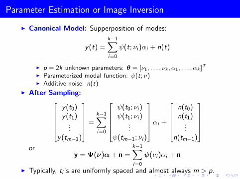
I Canonical Model: Supperposition of modes:
y(t) =k−1∑
i=0
ψ(t; νi )αi + n(t)
I p = 2k unknown parameters: θ = [ν1, . . . , νk , α1, . . . , αk ]T
I Parameterized modal function: ψ(t; ν)I Additive noise: n(t)
I After Sampling:
y(t0)y(t1)
...y(tm−1)
=
k−1∑
i=0
ψ(t0; νi )ψ(t1; νi )
...ψ(tm−1; νi )
αi +
n(t0)n(t1)
...n(tm−1)
ory = Ψ(ν)α+ n =
k−1∑
i=0
ψ(νi )αi + n
I Typically, ti ’s are uniformly spaced and almost always m > p.

Parameter Estimation or Image Inversion
I Canonical Model:
y = Ψ(ν)α+ n =k−1∑
i=0
ψ(νi )αi + n
I DOA estimation and spectrum analysis:
ψ(ν) = [e jt0ν , e jt1ν , . . . , e jtm−1ν ]T
where ν is the DOA (electrical angle) of a radiating point source.I Radar and sonar:
ψ(ν) = [w(t0 − τ)e jωt0 ,w(t1 − τ)e jωt1 , . . . ,w(tm−1 − τ)e jωtm−1 ]T
where w(t) is the transmit waveform and ν = (τ, ω) are delay andDoppler coordinates of a point scatterer.
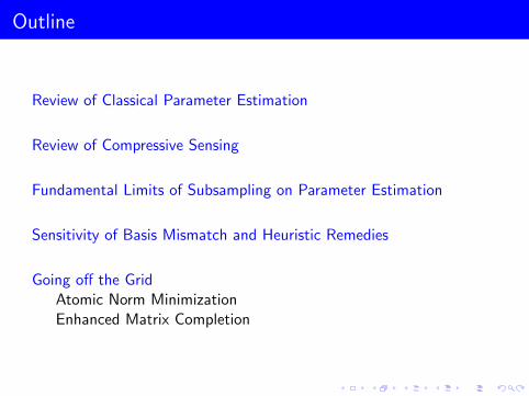
Outline
Review of Classical Parameter Estimation
Review of Compressive Sensing
Fundamental Limits of Subsampling on Parameter Estimation
Sensitivity of Basis Mismatch and Heuristic Remedies
Going off the GridAtomic Norm MinimizationEnhanced Matrix Completion
Outline
Review of Classical Parameter Estimation
Review of Compressive Sensing
Fundamental Limits of Subsampling on Parameter Estimation
Sensitivity of Basis Mismatch and Heuristic Remedies
Going off the GridAtomic Norm MinimizationEnhanced Matrix Completion

Classical Parameter Estimation or Image Inversion
I Matched filtering
I Sequence of rank-one subspaces, or 1D test images, is matched tothe measured image by filtering, correlating, or phasing.
I Test images are generated by scanning a prototype image (e.g., awaveform or a steering vector) through frequency, wavenumber,doppler, and/or delay at some desired resolution ∆ν.
P(`) = ‖ψ(`∆ν)Hy‖22
A. Pezeshki: Multi-rank MVDR Beamforming ISS Seminar, Princeton University, Feb. 1, 2007
Beamforming
A simple beamformer: Conventional (or Bartlett) beamformer
Sequence of plane-waves
Properties of the Bartlett beamformer:
Very simple Low resolution and high sidelobesGood interference suppression at some angles
Estimates the signal power
Matched Filtering
Bearing Response Cross-AmbiguityI Peak locations are taken as estimates of νi and peak values are
taken as estimates of source powers |αi |2.I Resolution: Rayleigh Limit (RL), inversely proportional to the
number of measurements

Classical Parameter Estimation or Image Inversion
I Matched filtering (Cont.)
I Extends to subspace matching for those cases in which the modelfor the image is comprised of several dominant modes.
I Extends to whitened matched filter, or minimum varianceunbiased (MVUB) filter, or generalized sidelobe canceller.
H. L. Van Trees, “Detection, Estimation, and Modulation Theory: Part I”,
D. J. Thomson, “Spectrum estimation and harmonic analysis,” Proc. IEEE, vol. 70, pp. 10551096, Sep. 1982.
T.-C.Lui and B. D. Van Veen, “Multiple window based minimum variance spectrum estimation formultidimensional random fields,” IEEE Trans. Signal Process., vol. 40, no. 3, pp. 578–589, Mar. 1992.
L. L. Scharf and B. Friedlander, “Matched subspace detectors,” IEEE Trans. Signal Process., vol. 42, no. 8, pp.21462157, Aug. 1994.
A. Pezeshki, B. D. Van Veen, L. L. Scharf, H. Cox, and M. Lundberg, “Eigenvalue beamforming using amulti-rank MVDR beamformer and subspace selection,” IEEE Trans. Signal Processing, vol. 56, no. 5, pp.1954–1967, May 2008.
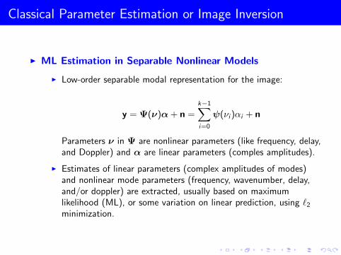
Classical Parameter Estimation or Image Inversion
I ML Estimation in Separable Nonlinear Models
I Low-order separable modal representation for the image:
y = Ψ(ν)α+ n =k−1∑
i=0
ψ(νi )αi + n
Parameters ν in Ψ are nonlinear parameters (like frequency, delay,and Doppler) and α are linear parameters (comples amplitudes).
I Estimates of linear parameters (complex amplitudes of modes)and nonlinear mode parameters (frequency, wavenumber, delay,and/or doppler) are extracted, usually based on maximumlikelihood (ML), or some variation on linear prediction, using `2
minimization.

Classical Parameter Estimation or Image Inversion
I Estimation of Complex Exponential ModesI Physical model:
y(t) =k−1∑
i=0
νti αi + n(t); ψ(t; νi ) = νti
where νi = edi+jωi is a complex exponential mode, with dampingdi and frequency ωi .
I Uniformly sampled measurement model:
y = Ψ(ν)α
Ψ(ν) =
ν00 ν0
1 · · · ν0k−1
ν10 ν1
1 · · · ν1k−1
ν20 ν2
1 · · · ν2k−1
......
. . ....
νm−10 νm−1
1 · · · νm−1k−1
.
Here, without loss of generality, we have taken the samples att = `t0, for ` = 0, 1, . . . ,m − 1, with t0 = 1.

Classical Parameter Estimation or Image Inversion
I ML Estimation of Complex Exponential Modes
minν,α‖y −Ψ(ν)α‖2
2
αML = Ψ(ν)†y
νML = argmin yHPA(ν)y; AHΨ = 0
Prony’s method (1795), modified leastsquares, linear prediction, and IterativeQuadratic Maximum Likelihood(IQML) are used to solve exact ML orits modifications. Rank-reduction isused to combat noise.
D. W. Tufts and R. Kumaresan, “Singular value decomposition and improved frequency estimation using linearprediction,” IEEE Trans. Acoust., Speech, Signal Process., vol. 30, no. 4, pp. 671675, Aug. 1982.
D. W. Tufts and R. Kumaresan, “Estimation of frequencies of mul- tiple sinusoids: Making linear predictionperform like maximum likelihood,” Proc. IEEE., vol. 70, pp. 975989, 1982.
L. L. Scharf “Statistical Signal Processing,” Prentice Hall, 1991.
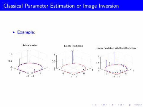
Classical Parameter Estimation or Image Inversion
I Example:
!1
0
1
!1
0
10
0.5
1
Actual modes
!1
0
1
!1
0
10
0.5
1
Conventional FFT
!1
0
1
!1
0
10
0.5
1
Compressed sensing
!1
0
1
!1
0
10
0.5
1
Linear Prediction
!1
0
1
!1
0
10
0.5
1
Actual modes
!1
0
1
!1
0
10
0.5
1
Conventional FFT
!1
0
1
!1
0
10
0.5
1
Compressed sensing
!1
0
1
!1
0
10
0.5
1
Linear Prediction
−10
1
−10
10
0.5
1
Actual modes
−10
1
−10
10
0.5
1
Conventional FFT
−10
1
−10
10
0.5
1
Compressed sensing
−10
1
−10
10
0.5
1
Linear Prediction with Rank Reduction
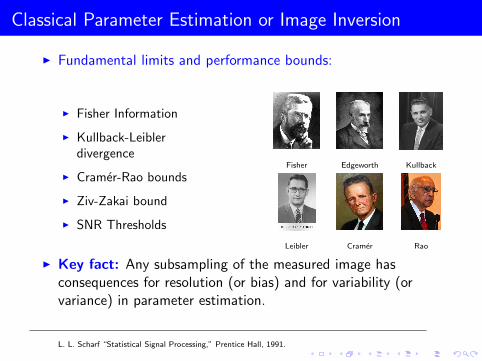
Classical Parameter Estimation or Image Inversion
I Fundamental limits and performance bounds:
I Fisher Information
I Kullback-Leiblerdivergence
I Cramer-Rao bounds
I Ziv-Zakai bound
I SNR Thresholds
Fisher Edgeworth Kullback
Leibler Cramer Rao
I Key fact: Any subsampling of the measured image hasconsequences for resolution (or bias) and for variability (orvariance) in parameter estimation.
L. L. Scharf “Statistical Signal Processing,” Prentice Hall, 1991.
Outline
Review of Classical Parameter Estimation
Review of Compressive Sensing
Fundamental Limits of Subsampling on Parameter Estimation
Sensitivity of Basis Mismatch and Heuristic Remedies
Going off the GridAtomic Norm MinimizationEnhanced Matrix Completion
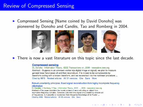
Review of Compressed Sensing
I Compressed Sensing [Name coined by David Donoho] waspioneered by Donoho and Candes, Tao and Romberg in 2004.
I There is now a vast literature on this topic since the last decade.
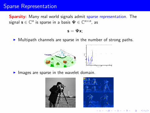
Sparse Representation
Sparsity: Many real world signals admit sparse representation. Thesignal s ∈ Cn is sparse in a basis Ψ ∈ Cn×n, as
s = Ψx;
I Multipath channels are sparse in the number of strong paths.
I Images are sparse in the wavelet domain.

Compression on the Fly
Compressed Sensing aims to characterize attributes of a signalwith a small number of measurements.
I Incoherence Sampling: the linear measurement y ∈ Cm isobtained via an incoherent matrix Φ ∈ Cm×n, as
y = Φs + n,
where m n. — subsampling.
I The goal is thus to recover x from y.

Uniqueness of Sparse Recovery
I Let A = ΦΨ ∈ Cm×n. We seek the sparsest signal satisfying theobservation:
(P0:) minx‖x‖0 subject to y = Ax.
where ‖ · ‖0 counts the number of nonzero entries.
I Spark: Let Spark(A) be the size of the smallest linearlydependent subset of columns of A.
Theorem (Uniqueness, Donoho and Elad 2002)
A representation y = Ax is necessarily the sparsest possible if‖x‖0 < Spark(A)/2.
Proof: If x and x′ satisfy Ax = Ax′, ‖x′‖0 ≤ ‖x‖0, thenA(x− x′) = 0 for ‖x− x′‖0 < Spark(A) implies x = x′.
D. Donoho and M. Elad, “Optimally sparse representation in general (nonorthogonal) dictionaries via `1minimization,” PNAS 100.5 (2003): 2197-2202.
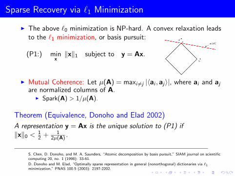
Sparse Recovery via `1 Minimization
I The above `0 minimization is NP-hard. A convex relaxation leadsto the `1 minimization, or basis pursuit:
I Mutual Coherence: Let µ(A) = maxi 6=j |〈ai , aj〉|, where ai and aj
are normalized columns of A.I Spark(A) > 1/µ(A).
Theorem (Equivalence, Donoho and Elad 2002)
A representation y = Ax is the unique solution to (P1) if‖x‖0 <
12 + 1
2µ(A) .
S. Chen, D. Donoho, and M. A. Saunders, “Atomic decomposition by basis pursuit,” SIAM journal on scientificcomputing 20, no. 1 (1998): 33-61.
D. Donoho and M. Elad, “Optimally sparse representation in general (nonorthogonal) dictionaries via `1minimization,” PNAS 100.5 (2003): 2197-2202.
(P1:) minx‖x‖1 subject to y = Ax.

Stable Sparse Recovery via Convex Relaxation
I When ‖n‖2 ≤ ε, we incorporate this into the basis pursuit:
(P1:) x∗ = arg minx‖x‖1 s.t. ‖y − Ax‖2 ≤ ε
I Restricted Isometry Property: If A satisfies the restrictedisometry property (RIP) with δ2k , then for any two k-sparsevectors x1 and x2:
1− δ2k ≤‖A(x1 − x2)‖2
2
‖x1 − x2‖22
≤ 1 + δ2k .
E. J. Candes, J. Romberg, and T. Tao, “Robust uncertainty principles: Exact signal reconstruction from highlyincomplete frequency information,” Information Theory, IEEE Transactions on 52.2 (2006): 489-509.Picture Credit: Mostafa Mohsenvand.
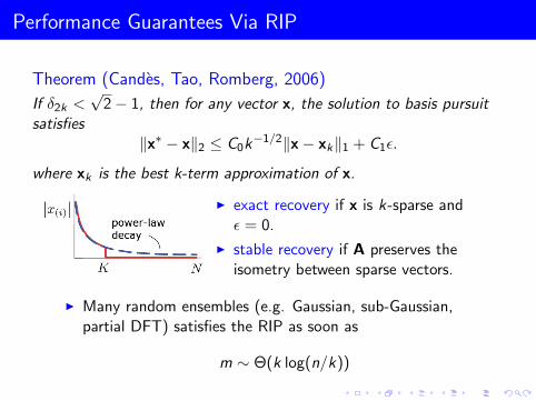
Performance Guarantees Via RIP
Theorem (Candes, Tao, Romberg, 2006)
If δ2k <√
2− 1, then for any vector x, the solution to basis pursuitsatisfies
‖x∗ − x‖2 ≤ C0k−1/2‖x− xk‖1 + C1ε.
where xk is the best k-term approximation of x.
I exact recovery if x is k-sparse andε = 0.
I stable recovery if A preserves theisometry between sparse vectors.
I Many random ensembles (e.g. Gaussian, sub-Gaussian,partial DFT) satisfies the RIP as soon as
m ∼ Θ(k log(n/k))
Extensions
I Recovery algorithms: Orthogonal Matching Pursuit (OMP),CoSaMP, Subspace Pursuit, Iterative Hard Thresholding,Bayesian inference, approximate message passing, etc...
I Refined signal models: tree sparsity, group sparsity, multiplemeasurements, etc...
I Measurement schemes: deterministic sensing matrices,structured random matrices, adaptive measurements, etc...

References
I The CS repository hosted by the DSP group at Rice University:http://dsp.rice.edu/cs
I The Nuite Blanche blog, maintained by Igor Carron, has awell-maintained list:https://sites.google.com/site/igorcarron2/cs
I Check the Nuite Blanche blog for recent updates:http://nuit-blanche.blogspot.com/

Outline
Review of Classical Parameter Estimation
Review of Compressive Sensing
Fundamental Limits of Subsampling on Parameter Estimation
Sensitivity of Basis Mismatch and Heuristic Remedies
Going off the GridAtomic Norm MinimizationEnhanced Matrix Completion
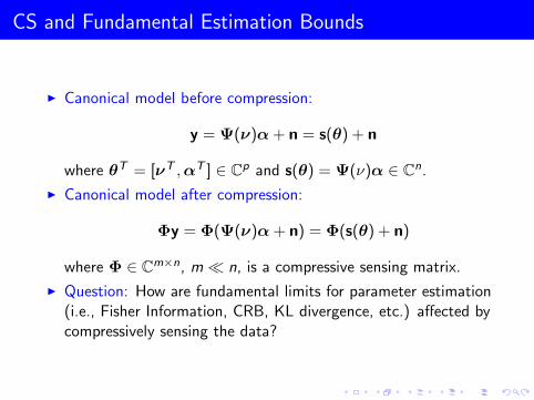
CS and Fundamental Estimation Bounds
I Canonical model before compression:
y = Ψ(ν)α+ n = s(θ) + n
where θT = [νT ,αT ] ∈ Cp and s(θ) = Ψ(ν)α ∈ Cn.
I Canonical model after compression:
Φy = Φ(Ψ(ν)α+ n) = Φ(s(θ) + n)
where Φ ∈ Cm×n, m n, is a compressive sensing matrix.
I Question: How are fundamental limits for parameter estimation(i.e., Fisher Information, CRB, KL divergence, etc.) affected bycompressively sensing the data?
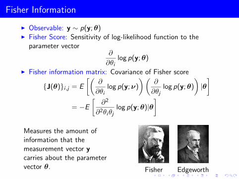
Fisher Information
I Observable: y ∼ p(y;θ)I Fisher Score: Sensitivity of log-likelihood function to the
parameter vector∂
∂θilog p(y;θ)
I Fisher information matrix: Covariance of Fisher score
J(θ)i ,j = E
[(∂
∂θilog p(y;ν)
)(∂
∂θjlog p(y;θ)
)|θ]
= −E
[∂2
∂2θiθjlog p(y;θ)|θ
]
Measures the amount ofinformation that themeasurement vector ycarries about the parametervector θ. Fisher Edgeworth

Cramer-Rao Lower Bound (CRB)
I Cramer-Rao lower bound: Lower bounds the error covariance ofany unbiased estimatior T (y) of the parameter vector θ frommeasurement y.
tr[covθ(T (y))] ≥ tr[J−1(θ)]
Cramer Rao
I The ith diagonal element of J−1(θ) lower bounds the MSE ofany unbiased estimator Ti (y) of the ith parameter θi from y.
I Volume of error concentration ellipse:
det[covθ(T (y))] ≥ det[J−1(θ)]
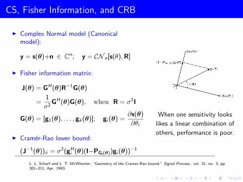
CS, Fisher Information, and CRB
I Complex Normal model (Canonicalmodel):
y = s(θ)+n ∈ Cn; y = CN n[s(θ),R]
I Fisher information matrix:
J(θ) = GH(θ)R−1G(θ)
=1
σ2GH(θ)G(θ), when R = σ2I
G(θ) = [g1(θ), . . . , gk(θ)]; gi (θ) =∂s(θ)
∂θi
I Cramer-Rao lower bound:
(J−1(θ))ii = σ2(gHi (θ)(I−PGi(θ))gi (θ))−1
When one sensitivity looks
likes a linear combination of
others, performance is poor.
L. L. Scharf and L. T. McWhorter, “Geometry of the Cramer-Rao bound,” Signal Process., vol. 31, no. 3, pp.301–311, Apr. 1993.

CS, Fisher Information, and CRB
I Compressive measurement(canonical model):
z = Φy = Φ[s(θ) + n] ∈ Cm;
I Fisher information matrix:
J(θ) =1
σ2GH(θ)PΦH G(ν) = GH(θ)G(θ)
G(θ) = [g1(θ), . . . , gk(θ)]; gi (θ) = PΦH
∂s(θ)
∂θi
I Cramer-Rao lower bound:
(J−1(θ))ii = σ2(gHi (θ)(I−PGi(θ))gi (θ))−1
Compressive measurement
reduces the distance between
subspaces: loss of information.
L. L. Scharf and L. T. McWhorter, “Geometry of the Cramer-Rao bound,” Signal Process., vol. 31, no. 3, pp.301–311, Apr. 1993.

CS, Fisher Information, and CRB
I Question: What is the impact of compressive sampling on theFisher information matrix and the Cramer-Rao bound (CRB) forestimating parameters?

CS, Fisher Information, and CRB
Theorem (Pakrooh, Pezeshki, Scharf, Chi ’13)
(a) For any compression matrix, we have
(J−1(θ))ii ≤ (J−1(θ))ii ≤ 1/λmin(GT (θ)PΦT G(θ))
(b) For a random compression matrix, we have
(J−1(θ))ii ≤λmax(J−1(θ))
C (1− ε)
with probability at least 1− δ − δ′.
Remarks:I (J−1)ii is the CRB in estimating the ith parameter θi .I CRB always gets worse after compressive sampling.I Theorem gives a confidence interval and a confidence level for
the increase in CRB after random compression.

CS, Fisher Information, and CRB
I δ satisfies
Pr(∀q ∈ 〈G(θ)〉 : (1− ε)‖q‖2
2 ≤ ‖Φq‖22 ≤ (1 + ε)‖q‖2
2
)≥ 1− δ.
I 1− δ′ is the probability that λmin((ΦΦT )−1) is larger than C .
I If entries of Φm×n are i.i.d. N (0, 1/m), then
I δ ≤ d(2√
p/ε′)pee−m(ε2/4−ε3/6), where
(3ε′
1− ε′ )2 + 2(
3ε′
1− ε′ ) = ε.
I δ′ is determined from the distribution of the largest eigenvalue ofa Wishart matrix, and the value of C , from a hypergeometricfunction.
P. Pakrooh, L. L. Scharf, A. Pezeshki and Y. Chi, “Analysis of Fisher information and the Cramer-Rao boundfor nonlinear parameter estimation after compressed sensing”, in Proc. 2013 IEEE Int. Conf. on Acoust.,Speech and Signal Process. (ICASSP), Vancouver May 26-31, 2013.

CRB after Compression
Example: Estimating the DOA of a point source at boresight θ1 = 0in the presence of a point interferer at electrical angle θ2.
I The LHS figure shows the after compassion CRB (red) for estimatingθ1 = 0 as θ2 is varied inside the (−2π/n, 2π/n] interval. Gaussiancompression is done from dimension n = 8192 to m = 3000.
I Bounds on the after compression CRB are shown in blue and black.The upper bounds in black hold with probability at least 1− δ − δ′,where δ′ = 0.05. An upper bound for δ versus the dimension of thecompression matrix is plotted on the RHS.
Kullback-Leibler (KL) Divergence
KL divergence: A non-symmetric measure of the difference betweentwo probability distributions
D(p(y;θ)||p(y;θ′)) =
∫
y
p(y;θ) logp(y;θ)
p(y;θ′)dy
Kullback Leilber
S. Kullback and R. A. Leibler, “On Information and Sufficiency,” Annals of Mathematical Statistics, vol. 22, no.1, pp. 79–86, 1951.
CS and KL Divergence
KL divergence between CN (s(θ),R) and CN (s(θ′),R):
D(θ,θ′) =1
2[(s(θ)− s(θ′))HR−1(s(θ)− s(θ′))].
I After compression with Φ:
D(θ,θ′) =1
2[(s(θ)− s(θ′))HΦH(ΦRΦH)−1Φ(s(θ)− s(θ′))].
I With white noise R = σ2I:
D(θ,θ′) =1
2σ2[(s(θ)− s(θ′))HPΦH (s(θ)− s(θ′))].
Theorem (Pakrooh, Pezeshki, Scharf, and Chi (ICASSP’13))
C (1− ε)D(θ,θ′) ≤ D(θ,θ′) ≤ D(θ,θ′)with probability at least 1− δ − δ′, where δ, δ′.
References on CS, Fisher Infromation, and CRB
I L. L. Scharf, E. K. P. Chong, A. Pezeshki, and J. R. Luo, “Compressivesensing and sparse inversion in signal processing: Cautionary notes,” inProc. 7th Workshop on Defence Applications of Signal Processing(DASP), Coolum, Queensland, Australia, Jul. 10-14, 2011.
I L. L. Scharf, E. K. P. Chong, A. Pezeshki, and J. R. Luo, “Sensitivityconsiderations in compressed sensing,” in Conf. Rec. 45th AnnualAsilomar Conf. Signals, Systs., Computs., Pacific Grove, CA,, Nov.2011, pp. 744–748.
I P. Pakrooh, L. L. Scharf, A. Pezeshki and Y. Chi, “Analysis of Fisherinformation and the Cramer-Rao bound for nonlinear parameterestimation after compressed sensing”, in Proc. 2013 IEEE Int. Conf.on Acoust., Speech and Signal Process. (ICASSP), Vancouver May26-31, 2013.
Work by Others
I Nielsen, Christensen, and Jensen (ICASSP’12): Bounds on meanvalue of Fisher Information after random compression.
I Ramasamy, Venkateswaran, and Madhow (Asilomar’12): Boundson Fisher information after compression in a different noisymodel.
I Babadi, Kalouptsidis, and Tarokh (TSP 2009): Existence of anestimator (“Joint Typicality Estimator”) that asymptoticallyachieves the CRB in linear parameter estimation with randomGaussian compression matrices.
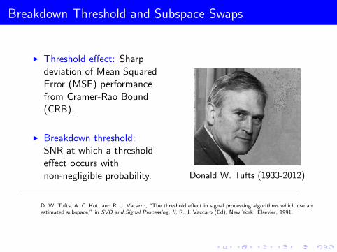
Breakdown Threshold and Subspace Swaps
I Threshold effect: Sharpdeviation of Mean SquaredError (MSE) performancefrom Cramer-Rao Bound(CRB).
I Breakdown threshold:SNR at which a thresholdeffect occurs withnon-negligible probability. Donald W. Tufts (1933-2012)
D. W. Tufts, A. C. Kot, and R. J. Vacarro, “The threshold effect in signal processing algorithms which use anestimated subspace,” in SVD and Signal Processing, II, R. J. Vaccaro (Ed), New York: Elsevier, 1991.
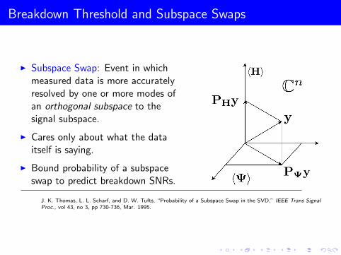
Breakdown Threshold and Subspace Swaps
I Subspace Swap: Event in whichmeasured data is more accuratelyresolved by one or more modes ofan orthogonal subspace to thesignal subspace.
I Cares only about what the dataitself is saying.
I Bound probability of a subspaceswap to predict breakdown SNRs.
J. K. Thomas, L. L. Scharf, and D. W. Tufts, “Probability of a Subspace Swap in the SVD,” IEEE Trans SignalProc., vol 43, no 3, pp 730-736, Mar. 1995.

Signal Model: Mean Case
I Before compression:
y : CN n[Ψα, σ2I]; Ψ ∈ Cn×k
I After compression with compressive sensing matrixΦcs ∈ Cm×n,m < n:
ycs : CNm[ΦcsΨα, σ2ΦcsΦ
Hcs ]
or equivalently (with some abuse of notation):
ycs : CNm[ΦΨα, σ2I], Φ = (ΦcsΦHcs)−1/2Φcs

Subspace Swap Events
I Subspace Swap Event E : One or more modes of the orthogonalsubspace 〈H〉 resolves more energy than one or more modes ofthe noise-free signal subspace 〈Ψ〉.

Subspace Swap Events
I Subevent F : Average energy resolved in the orthogonal subspace〈H〉 = 〈Ψ〉⊥ is greater than the average energy resolved in thenoise-free signal subspace 〈Ψ〉.
mini|ψH
i y|2 ≤1
kyHPΨy <
1
n − kyHPHy≤ max
i|hH
i y|2
I Subevent G : Energy resolved in the apriori minimum mode ψmin
of the noise-free signal subspace 〈Ψ〉 is smaller than the averageenergy resolved in the orthogonal subspace 〈H〉.
|ψHminy|2 < 1
n − kyHPHy≤ max
i|hH
i y|2.
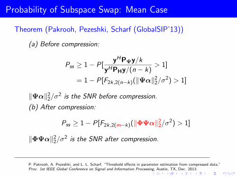
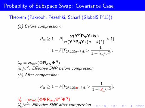
Probability of Subspace Swap: Mean Case
Theorem (Pakrooh, Pezeshki, Scharf (GlobalSIP’13))
(a) Before compression:
Pss ≥ 1− P[yHPΨy/k
yHPHy/(n − k)> 1]
= 1− P[F2k,2(n−k)(‖Ψα‖22/σ
2) > 1]
‖Ψα‖22/σ
2 is the SNR before compression.
(b) After compression:
Pss ≥ 1− P[F2k,2(m−k)(‖ΦΨα‖22/σ
2) > 1]
‖ΦΨα‖22/σ
2 is the SNR after compression.
P. Pakrooh, A. Pezeshki, and L. L. Scharf, “Threshold effects in parameter estimation from compressed data,”Proc. 1st IEEE Global Conference on Signal and Information Processing, Austin, TX, Dec. 2013.

Sensor Array Processing–Mean Case
−30 −25 −20 −15 −10 −5 0 5 100
0.1
0.2
0.3
0.4
0.5
0.6
0.7
SNR (dB)
Pss
AC
BC
−30 −25 −20 −15 −10 −5 0 5 10−70
−60
−50
−40
−30
−20
−10
0
SNR (dB)
MS
E (
dB
)
ML: AC
Approx: AC
ML: BC
Approx: BC
CRB: AC
CRB: BC
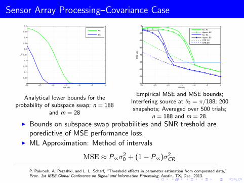
Analytical lower bounds for theprobability of subspace swap. Array size:n = 188 elements; Compressed array
m = 28 elements.
Empirical MSE (average over 200 trials)and MSE bounds for estimating θ1 = 0;Interfering source at θ2 = π/188; Arraysize: n = 188 elements; Compressed
array m = 28 elements.
I Bounds on subspace swap probabilities and SNR treshold areporedictive of MSE performance loss.
I ML Approximation: Method of intervals
MSE ≈ Pssσ20 + (1− Pss)σ2
CR
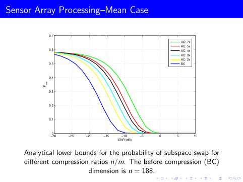
Sensor Array Processing–Mean Case
−30 −25 −20 −15 −10 −5 0 5 100
0.1
0.2
0.3
0.4
0.5
0.6
0.7
SNR (dB)
Pss
AC: 7x
AC: 5x
AC: 4x
AC: 3x
AC: 2x
BC
Analytical lower bounds for the probability of subspace swap fordifferent compression ratios n/m. The before compression (BC)
dimension is n = 188.

Signal Model: Covariance Case
I Before compression:
y : CN n[0,ΨRααΨH + σ2I]; Ψ ∈ Cn×k
I After compression with compressive sensing matrixΦcs ∈ Cm×n,m < n:
ycs : CNm[0,ΦcsΨRααΨHΦH
cs + σ2ΦcsΦHcs ]
or equivalently (with some abuse of notation):
ycs : CNm[0,ΦΨRααΦΨH + σ2I], Φ = (ΦcsΦHcs)−1/2Φcs .
I Assume data consists of L iid realizations of y arranged asY = [y1, y2, · · · , yL].
Probablity of Subspace Swap: Covariance Case
Theorem (Pakrooh, Pezeshki, Scharf (GlobalSIP’13))
(a) Before compression:
Pss ≥ 1− P[tr(YHPΨY/kL)
tr(YHPHY/(n − k)L)> 1]
= 1− P[F2kL,2(n−k)L >1
1 + λk/σ2].
λk = evmin(ΨRααΨH)
λk/σ2: Effective SNR before compression
(b) After compression:
Pss ≥ 1− P[F2kL,2(m−k)L >1
1 + λ′k/σ2
].
λ′k = evmin(ΦΨRααΨHΦH)
λ′k/σ2: Effective SNR after compression
Sensor Array Processing–Covariance Case
−30 −25 −20 −15 −10 −5 00
0.05
0.1
0.15
0.2
0.25
0.3
0.35
0.4
0.45
0.5
SNR (dB)
Pss
AC
BC
−30 −25 −20 −15 −10 −5 0−80
−70
−60
−50
−40
−30
−20
−10
0
SNR(dB)
MS
E (
dB
)
ML: AC
Approx: AC
ML: BC
Approx: BC
CRB: AC
CRB: BC
Analytical lower bounds for theprobability of subspace swap; n = 188
and m = 28
Empirical MSE and MSE bounds;Interfering source at θ2 = π/188; 200snapshots; Averaged over 500 trials;
n = 188 and m = 28.I Bounds on subspace swap probabilities and SNR treshold are
poredictive of MSE performance loss.I ML Approximation: Method of intervals
MSE ≈ Pssσ20 + (1− Pss)σ2
CR
P. Pakrooh, A. Pezeshki, and L. L. Scharf, “Threshold effects in parameter estimation from compressed data,”Proc. 1st IEEE Global Conference on Signal and Information Processing, Austin, TX, Dec. 2013.
References on Breakdown Thresholds
I P. Pakrooh, A. Pezeshki, and L. L. Scharf, “Threshold effects inparameter estimation from compressed data,” Proc. 1st IEEE GlobalConference on Signal and Information Processing, Austin, TX, Dec.2013.
I D. Tufts, A. Kot, and R. Vaccaro, The threshold effect in signalprocessing algorithms which use an estimated subspace, SVD andSignal Processing II: Algorithms, Analysis and Applications, New York:Elsevier, 1991, pp. 301320.
I J. K. Thomas, L. L. Scharf, and D. W. Tufts, The probability of asubspace swap in the SVD, IEEE Transactions on Signal Processing,vol. 43, no. 3, pp. 730736, Mar. 1995.
I B. A. Johnson, Y. I. Abramovich, and X. Mestre, MUSIC, G-MUSIC,and maximum-likelihood performance breakdown, IEEE Transactionson Signal Processing, vol. 56, no. 8, pp. 3944-3958, Aug. 2008.

Intermediate Recap: Fundamental Limits
I Compression (even with Gaussian or similar random matrices)has performance consequences.
I The CR bound increases and the onset of threshold SNRincreases. These increases may be quantified to determine wherecompressive sampling is viable.

Outline
Review of Classical Parameter Estimation
Review of Compressive Sensing
Fundamental Limits of Subsampling on Parameter Estimation
Sensitivity of Basis Mismatch and Heuristic Remedies
Going off the GridAtomic Norm MinimizationEnhanced Matrix Completion

Basis Mismatch: NonLin. Overdet. vs. Lin. Underdet.
I Convert the nonlinear problem into a linear system viadiscretization of the parameter space at desired resolution:
s(θ) =k−1∑
i=0
ψ(νi )αi
= Ψphα
Over-determined &nonlinear
s ≈ [ψ(ω1), · · · ,ψ(ωn)]
x1
...xn
= Ψcsx
Under-determined linear &sparse
I The set of candidate νi ∈ Ω is quantized to Ω = ω1, · · · , ωn,n > m; Ψph unknown and Ψcs assumed known.

Basis Mismatch: A Tale of Two Models
Mathematical (CS) model:
s = Ψcsx
The basis Ψcs is assumed,typically a gridded imagingmatrix (e.g., n point DFTmatrix or identity matrix), andx is presumed to be k-sparse.
Physical (true) model:
s = Ψphα
The basis Ψph is unknown, andis determined by a point spreadfunction, a Green’s function, oran impulse response, and α isk-sparse and unknown.
Key transformation:
x = Ψmisα = Ψ−1cs Ψphα
x is sparse in the unknownΨmis basis, not in the identitybasis.

Basis Mismatch: From Sparse to Incompressible
DFT Grid Mismatch:
Ψmis = Ψ−1cs Ψph =
L(∆θ0 − 0) L(∆θ1 − 2π(n−1)n
) · · · L(∆θn−1 − 2πn
)
L(∆θ0 − 2πn
) L(∆θ1 − 0) · · · L(∆θn−1 − 2π·2n
)
.
.
.
.
.
.. . .
.
.
.
L(∆θ0 − 2π(n−1)n
) L(∆θ1 − 2π(n−2)n
) · · · L(∆θn−1 − 0)
where L(θ) is the Dirichlet kernel:
L(θ) =1
n
n−1∑
`=0
e j`θ =1
ne j θ(n−1)
2sin(θn/2)
sin(θ/2).
−10 −5 0 5 10−0.4
−0.2
0
0.2
0.4
0.6
0.8
1
θ/(2π/N)
sin(N
θ/2)
Nsin(θ/2)
Slow decay of theDirichlet kernel meansthat the presumablysparse vectorx = Ψmisα is in factincompressible.

Basis Mismatch: Fundamental Question
Question: What is the consequence of assuming that x is k-sparse inI, when in fact it is only k-sparse in an unknown basis Ψmis , which isdetermined by the mismatch between Ψcs and Ψph?
. . . . . .
Basis Mismatch
Two models:
s = !0x = !1!
Key transformation:
x = !! = !!10 !1!
x is sparse in the unknown ! basis, not in the identity basis.
Physical Model CS InverterCS Sampler
y = !s
min !x!1
s.t. y = !"csxs = "ph"
() June 25, 2014 1 / 1
Sensitivity to Basis Mismatch
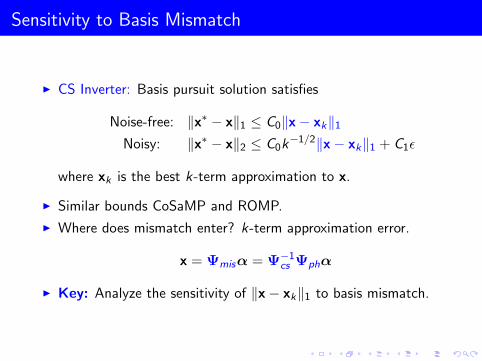
I CS Inverter: Basis pursuit solution satisfies
Noise-free: ‖x∗ − x‖1 ≤ C0‖x− xk‖1
Noisy: ‖x∗ − x‖2 ≤ C0k−1/2‖x− xk‖1 + C1ε
where xk is the best k-term approximation to x.
I Similar bounds CoSaMP and ROMP.
I Where does mismatch enter? k-term approximation error.
x = Ψmisα = Ψ−1cs Ψphα
I Key: Analyze the sensitivity of ‖x− xk‖1 to basis mismatch.
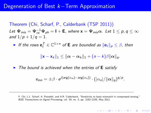
Degeneration of Best k−Term Approximation
Theorem (Chi, Scharf, P., Calderbank (TSP 2011))
Let Ψmis = Ψ−1cs Ψph = I + E, where x = Ψmisα. Let 1 ≤ p, q ≤ ∞
and 1/p + 1/q = 1.
I If the rows eT` ∈ C1×n of E are bounded as ‖e`‖p ≤ β, then
‖x− xk‖1 ≤ ‖α−αk‖1 + (n − k)β‖α‖q.
I The bound is achieved when the entries of E satisfy
emn = ±β · e j(arg(αm)−arg(αn)) · (|αn|/‖α‖q)q/p.
Y. Chi, L.L. Scharf, A. Pezeshki, and A.R. Calderbank, “Sensitivity to basis mismatch in compressed sensing,”IEEE Transactions on Signal Processing, vol. 59, no. 5, pp. 2182–2195, May 2011.
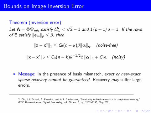
Bounds on Image Inversion Error
Theorem (inversion error)
Let A = ΦΨmis satisfy δA2k <
√2− 1 and 1/p + 1/q = 1. If the rows
of E satisfy ‖em‖p ≤ β, then
‖x− x∗‖1 ≤ C0(n − k)β‖α‖q. (noise-free)
‖x− x∗‖2 ≤ C0(n − k)k−1/2β‖α‖q + C1ε. (noisy)
I Message: In the presence of basis mismatch, exact or near-exactsparse recovery cannot be guaranteed. Recovery may suffer largeerrors.
Y. Chi, L.L. Scharf, A. Pezeshki, and A.R. Calderbank, “Sensitivity to basis mismatch in compressed sensing,”IEEE Transactions on Signal Processing, vol. 59, no. 5, pp. 2182–2195, May 2011.
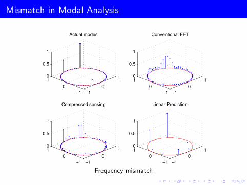
Mismatch in Modal Analysis
−1
0
1
−1
0
10
0.5
1
Actual modes
−1
0
1
−1
0
10
0.5
1
Conventional FFT
−1
0
1
−1
0
10
0.5
1
Compressed sensing
−1
0
1
−1
0
10
0.5
1
Linear Prediction
Frequency mismatch

Mismatch in Modal Analysis
−1
0
1
−1
0
10
0.5
1
Actual modes
−1
0
1
−1
0
10
0.5
1
Conventional FFT
−1
0
1
−1
0
10
0.5
1
Compressed sensing
−1
0
1
−1
0
10
0.5
1
Linear Prediction
Damping mismatch

Mismatch in Modal Analysis
−1
0
1
−1
0
10
0.5
1
Actual modes
−1
0
1
−1
0
10
0.5
1
Conventional FFT
−1
0
1
−1
0
10
0.5
1
Compressed sensing
−1
0
1
−1
0
10
0.5
1
Linear Prediction with Rank Reduction
Frequency mismatch–noisy measurements

Mismatch in Modal Analysis
But what if we make the grid finer and finer?I Over-resolution experiment:
I m = 25 samples
I Equal amplitude complex tones at f1 = 0.5 Hz and f2 = 0.52 Hz(half the Rayleigh limit apart), mismatched to mathematical basis.
I Mathematical model is s = Ψcsx, where Ψcs is the m × n, withn = mL, “DFT” frame that is over-resolved to ∆f = 1/mL.
Ψcs =1√m
1 1 · · · 1
1 e j 2πmL · · · e j 2π(mL−1)
mL
......
. . ....
1 e j 2π(m−1)mL · · · e j 2π(m−1)(mL−1)
mL
.
I What we will see:I MSE of inversion is noise-defeated, noise-limited, quantization
limited, or null-space limited—depending on SNR.
L. L. Scharf, E. K. P. Chong, A. Pezeshki, and J. R. Luo, “Sensitivity considerations in compressed sensing,” inConf. Rec. Asilomar’11, Pacific Grove, CA,, Nov. 2011, pp. 744–748.
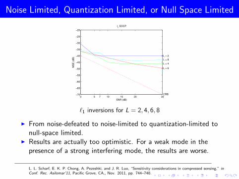
Noise Limited, Quantization Limited, or Null Space Limited
0 5 7 10 15 20 30−70
−65
−60
−55
−50
−45
−40
−35
−30
−25
−20
CRB
l1 SOCP
SNR (dB)
MS
E (
dB
) L = 2
L = 4
L = 6
L = 8
`1 inversions for L = 2, 4, 6, 8
I From noise-defeated to noise-limited to quantization-limited tonull-space limited.
I Results are actually too optimistic. For a weak mode in thepresence of a strong interfering mode, the results are worse.
L. L. Scharf, E. K. P. Chong, A. Pezeshki, and J. R. Luo, “Sensitivity considerations in compressed sensing,” inConf. Rec. Asilomar’11, Pacific Grove, CA,, Nov. 2011, pp. 744–748.
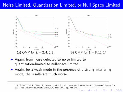
Noise Limited, Quantization Limited, or Null Space Limited
0 5 7 10 15 20 30−70
−65
−60
−55
−50
−45
−40
−35
−30
−25
−20
CRB
OMP
SNR (dB)
MS
E (
dB
) L = 2
L = 4
L = 6
L = 8
0 5 7 10 15 20 30−70
−65
−60
−55
−50
−45
−40
−35
−30
−25
−20
CRB
OMP
SNR (dB)
MS
E (
dB
)
L = 8
L = 12
L = 14
(a) OMP for L = 2, 4, 6, 8 (b) OMP for L = 8, 12, 14
I Again, from noise-defeated to noise-limited toquantization-limited to null-space limited.
I Again, for a weak mode in the presence of a strong interferingmode, the results are much worse.
L. L. Scharf, E. K. P. Chong, A. Pezeshki, and J. R. Luo, “Sensitivity considerations in compressed sensing,” inConf. Rec. Asilomar’11, Pacific Grove, CA,, Nov. 2011, pp. 744–748.

Scatter Plots for BPDN Estimates
I Scatter plots for the normalized errors in estimating the sum anddifference frequencies using BPDN.
−0.03 −0.02 −0.01 0 0.01 0.02 0.03−0.03
−0.02
−0.01
0
0.01
0.02
0.03
l1 with SNR = 7 dB
f1 estimation error
f 2 e
stim
atio
n e
rro
r
L = 2
L = 5
L = 9
−0.1 −0.05 0 0.05 0.1−1
−0.5
0
0.5
1
1.5
2
l1 with SNR = 7 dB
Normalized sum of estimates
No
rma
lize
d d
iffe
ren
ce
of
estim
ate
s
L = 2
L = 5
L = 9
(a) (f1 + f2) (b) (f1 − f2)
I At L = 2 mean-squared error is essentially bias-squared, whereas forL = 9 it is essentially variance.
I Average frequency is easy to estimate, but the difference frequency ishard to estimate. (Vertical scale is nearly 10 times the horizontal scale.)
I BPDN favors large negative differences over large positive differences(better estimates the mode at f1 than it estimates the mode at f2).

Scatter Plots for OMP Estimates
I Scatter plots for the normalized errors in estimating the sum anddifference frequencies using BPDN.
−0.03 −0.02 −0.01 0 0.01 0.02 0.03−0.03
−0.02
−0.01
0
0.01
0.02
0.03
OMP with SNR = 7 dB
f1 estimation error
f 2 e
stim
atio
n e
rro
r
L = 2
L = 9
L = 19
−0.1 −0.05 0 0.05 0.1−1
−0.5
0
0.5
1
1.5
2
OMP with SNR = 7 dB
Normalized sum of estimates
No
rma
lize
d d
iffe
ren
ce
of
estim
ate
s
L = 2
L = 5
L = 9
(a) (f1 + f2) (b) (f1 − f2)
I Preference for large negative errors in estimating the differencefrequency disappears.
I Correlation between sum and difference errors reflects the fact that alarge error in extracting the first mode will produce a large error inextracting the second.

References on Model Mismatch in CS
I Y. Chi, A. Pezeshki, L. L. Scharf, and R. Calderbank, “Sensitivity tobasis mismatch in compressed sensing,” in Proc. ICASSP’10, Dallas,TX, Mar. 2010, pp. 3930 –3933.
I Y. Chi, L.L. Scharf, A. Pezeshki, and A.R. Calderbank, “Sensitivity tobasis mismatch in compressed sensing,” IEEE Transactions on SignalProcessing, vol. 59, no. 5, pp. 2182–2195, May 2011.
I L. L. Scharf, E. K. P. Chong, A. Pezeshki, and J. R. Luo, “Compressivesensing and sparse inversion in signal processing: Cautionary notes,” inProc. DASP’11, Coolum, Queensland, Australia, Jul. 10-14, 2011.
I L. L. Scharf, E. K. P. Chong, A. Pezeshki, and J. R. Luo, “Sensitivityconsiderations in compressed sensing,” in Conf. Rec. Asilomar’11,Pacific Grove, CA,, Nov. 2011, pp. 744–748.
I M. A. Herman and T. Strohmer, “General deviants: An analysis ofperturbations in compressed sensing,” IEEE J. Selected Topics inSignal Processing, vol. 4, no. 2, pp. 342349, Apr. 2010.
I D. H Chae, P. Sadeghi, and R. A. Kennedy, “Effects of basis-mismatchin compressive sampling of continuous sinusoidal signals,” Proc. Int.Conf. on Future Computer and Commun., Wuhan, China, May 2010.

Remedies to Basis Mismatch : A Partial List
These approaches still assume a grid.
I H. Zhu, G. Leus, and G. B. Giannakis, “Sparsity-cognizant totalleast-squares for perturbed compressive sampling,” IEEE Transactionson Signal Processing, vol. 59, May 2011.
I M. F. Duarte and R. G. Baraniuk, “Spectral compressive sensing,”Applied and Computational Harmonic Analysis, Vol. 35, No. 1, pp.111-129, 2013.
I A. Fannjiang and W. Liao, “Coherence-Pattern Guided CompressiveSensing with Unresolved Grids,” SIAM Journal of Imaging Sciences,Vol. 5, No. 1, pp. 179-202, 2012.
Intermediate Recap: Sensitivity of CS to Basis Mismatch
I Basis mismatch is inevitable and sensitivities of CS to basismismatch need to be fully understood. No matter how finely wegrid the parameter space, the actual modes almost never lie onthe grid.
I The consequence of over-resolution (very fine gridding) is thatperformance follows the Cramer-Rao bound more closely at lowSNR, but at high SNR it departs more dramatically from theCramer-Rao bound.
I This matches intuition that has been gained from moreconventional modal analysis where there is a qualitatively similartrade-off between bias and variance. That is, bias may bereduced with frame expansion (over-resolution), but there is apenalty to be paid in variance.
Outline
Review of Classical Parameter Estimation
Review of Compressive Sensing
Fundamental Limits of Subsampling on Parameter Estimation
Sensitivity of Basis Mismatch and Heuristic Remedies
Going off the GridAtomic Norm MinimizationEnhanced Matrix Completion
Going Off the Grid
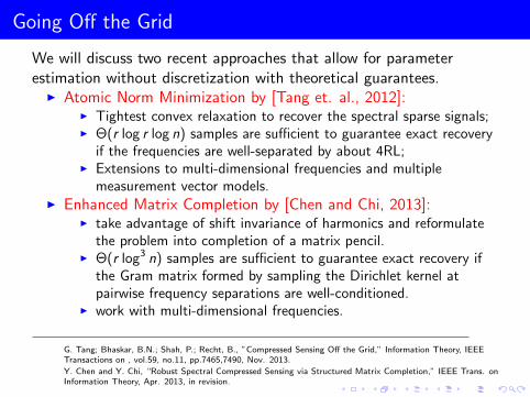
We will discuss two recent approaches that allow for parameterestimation without discretization with theoretical guarantees.
I Atomic Norm Minimization by [Tang et. al., 2012]:I Tightest convex relaxation to recover the spectral sparse signals;I Θ(r log r log n) samples are sufficient to guarantee exact recovery
if the frequencies are well-separated by about 4RL;I Extensions to multi-dimensional frequencies and multiple
measurement vector models.I Enhanced Matrix Completion by [Chen and Chi, 2013]:
I take advantage of shift invariance of harmonics and reformulatethe problem into completion of a matrix pencil.
I Θ(r log3 n) samples are sufficient to guarantee exact recovery ifthe Gram matrix formed by sampling the Dirichlet kernel atpairwise frequency separations are well-conditioned.
I work with multi-dimensional frequencies.
G. Tang; Bhaskar, B.N.; Shah, P.; Recht, B., ”Compressed Sensing Off the Grid,” Information Theory, IEEETransactions on , vol.59, no.11, pp.7465,7490, Nov. 2013.
Y. Chen and Y. Chi, “Robust Spectral Compressed Sensing via Structured Matrix Completion,” IEEE Trans. onInformation Theory, Apr. 2013, in revision.
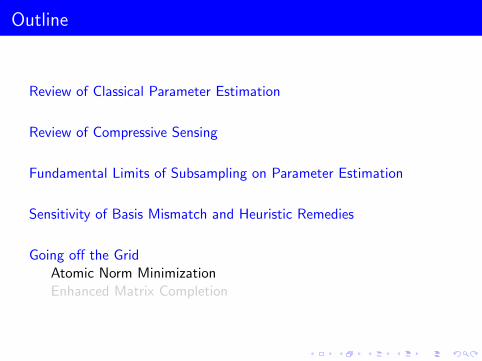
Outline
Review of Classical Parameter Estimation
Review of Compressive Sensing
Fundamental Limits of Subsampling on Parameter Estimation
Sensitivity of Basis Mismatch and Heuristic Remedies
Going off the GridAtomic Norm MinimizationEnhanced Matrix Completion

The Atomic Norm Approach
The atomic norm is proposed to find tightest convex relaxations ofgeneral parsimonious models including sparse signals as a special case.The prescribed recipe is:
I Step 1: assume the signal of interest can be written as asuperposition of small numbers of atoms in A:
x =r∑
i=1
ciai , ai ∈ A, ci > 0.
I Step 2: define the atomic norm of the signal as:
‖x‖A = inf t > 0 : x ∈ tconv(A)
= inf
∑
i
ci
∣∣∣x =∑
i
ciai , ai ∈ A, ci > 0
.
I Step 3: formulate a convex program to minimize the atomicnorm with respect to the measurements.
Chandrasekaran, V., B. Recht, P. A. Parrilo, and A. S. Willsky. ”The convex geometry of linear inverseproblems.” Foundations of Computational Mathematics 12, no. 6 (2012): 805-849.

Examples: The Atomic Norm Approach
Several popular approaches become special cases of the atomic normminimization framework.
I Sparse signals: an atom for sparse signals is a normalized vectorof sparsity one, and the atomic norm is `1 norm;
I Low-rank matrices: an atom for low-rank matrices is anormalized rank-one matrix; and the atomic norm is nuclearnorm;
(a) unit ball of `1 norm (b) unit ball of nuclear norm
Chandrasekaran, V., B. Recht, P. A. Parrilo, and A. S. Willsky. ”The convex geometry of linear inverseproblems.” Foundations of Computational Mathematics 12, no. 6 (2012): 805-849.

Atomic Norm For Spectrally-Sparse Signals
I Let x(t) =∑r
i=1 diej2πfi t , fi ∈ [0, 1), t = 0, . . . , n − 1. Denote
F = firi=1.
I Stack x(t) into a vector x: x =∑r
i=1 dia(fi ), di ∈ C where a(f )is the atom defined as
a(f ) =1√n
[1 e j2πf . . . e j2πf (n−1)
].
I Atomic norm:
‖x‖A = inf
∑
k
|ck |∣∣∣x =
∑
k
cka(fk), fk ∈ [0, 1)
= infu,t
1
2Tr(toep(u)) +
1
2t∣∣∣[toep(u) x
x∗ t
] 0
.
which can be equivalently given in an SDP form.
G. Tang; Bhaskar, B.N.; Shah, P.; Recht, B., ”Compressed Sensing Off the Grid,” Information Theory, IEEETransactions on , vol.59, no.11, pp.7465,7490, Nov. 2013.
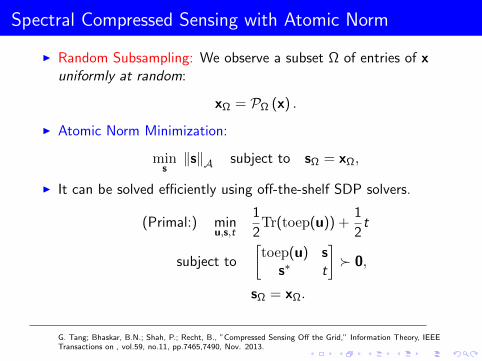
Spectral Compressed Sensing with Atomic Norm
I Random Subsampling: We observe a subset Ω of entries of xuniformly at random:
xΩ = PΩ (x) .
I Atomic Norm Minimization:
mins‖s‖A subject to sΩ = xΩ,
I It can be solved efficiently using off-the-shelf SDP solvers.
(Primal:) minu,s,t
1
2Tr(toep(u)) +
1
2t
subject to
[toep(u) s
s∗ t
] 0,
sΩ = xΩ.
G. Tang; Bhaskar, B.N.; Shah, P.; Recht, B., ”Compressed Sensing Off the Grid,” Information Theory, IEEETransactions on , vol.59, no.11, pp.7465,7490, Nov. 2013.
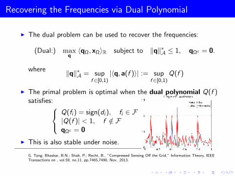
Recovering the Frequencies via Dual Polynomial
I The dual problem can be used to recover the frequencies:
(Dual:) maxq〈qΩ, xΩ〉R subject to ‖q‖∗A ≤ 1, qΩc = 0.
where ‖q‖∗A = supf ∈[0,1)
|〈q, a(f )〉| := supf ∈[0,1)
Q(f )
I The primal problem is optimal when the dual polynomial Q(f )satisfies:
Q(fi ) = sign(di ), fi ∈ F|Q(f )| < 1, f /∈ FqΩc = 0
I This is also stable under noise.
G. Tang; Bhaskar, B.N.; Shah, P.; Recht, B., ”Compressed Sensing Off the Grid,” Information Theory, IEEETransactions on , vol.59, no.11, pp.7465,7490, Nov. 2013.

Performance Guarantees for Noiseless Recovery
Theorem (Tang et. al., 2012)
Suppose a subset of m entries are observed uniformly at random.Additionally, assume the phase of the coefficients are drawn i.i.d.from the uniform distribution on the complex unit circle and
∆ = minfj 6=fk|fj − fk | ≥
1
b(n − 1)/4c ,
then m ≥ C
log2 nδ , r log n
δ log rδ
is sufficient to guarantee exact
recovery with probability at least 1− δ with respect to the randomsamples and signs, where C is some numerical constant.
I Random data model, and random observation model.I m = Θ(r log n log r) samples suffice if a separation condition of
about 4RL is satisfied.
G. Tang; Bhaskar, B.N.; Shah, P.; Recht, B., ”Compressed Sensing Off the Grid,” Information Theory, IEEETransactions on , vol.59, no.11, pp.7465,7490, Nov. 2013.

Phase Transition
Figure : Phase transition diagrams when n = 128 and the separation is setto be 1.5 RL. Both signs and magnitudes of the coeffients are random.
G. Tang; Bhaskar, B.N.; Shah, P.; Recht, B., ”Compressed Sensing Off the Grid,” Information Theory, IEEETransactions on , vol.59, no.11, pp.7465,7490, Nov. 2013.

Extension for MMV Models
I For multiple spectrally-sparse signals X =∑r
i=1 a(fi )b∗i ∈ Cn×L,we define the atomic set A composed of atoms as
A(f ,b) = a(f )b∗ ∈ Cn×L, ‖b‖2 = 1.
I The atomic norm is defined and computed as [Chi, 2013]
‖X‖A = inf
∑
k
ck∣∣X =
∑
k
ckA(fk ,bk), ck ≥ 0
= infu,W
1
2Tr(toep(u)) +
1
2Tr(W)
∣∣∣[toep(u) X
X∗ W
] 0
.
I The single vector case becomes a special case when L = 1. Thealgorithm is tractable however the complexity might become highwhen L is large.
Y. Chi, “Joint Sparsity Recovery for Spectral Compressed Sensing”, in International Conference on Acoustics,Speech, and Signal Processing (ICASSP), Florence, Italy, May 2014.

Two-Dimensional Frequency Model
I Stack x (t) =∑r
i=1 diej2π〈t,fi 〉 into a matrix X ∈ Cn1×n2 .
I The matrix X has the following Vandermonde decomposition:
X = Y · D︸︷︷︸diagonal matrix
· ZT .
Here, D := diag d1, · · · , dr and
Y :=
1 1 · · · 1y1 y2 · · · yr...
......
...
yn1−11 yn1−1
2 · · · yn1−1r
︸ ︷︷ ︸
Vandemonde matrix
,Z :=
1 1 · · · 1z1 z2 · · · zr...
......
...
zn2−11 zn2−1
2 · · · zn2−1r
︸ ︷︷ ︸
Vandemonde matrix
where yi = exp(j2πf1i ), zi = exp(j2πf2i ), fi = (f1i , f2i ).
I Goal: We observe a random subset of entries of X, and wish torecover the missing entries.
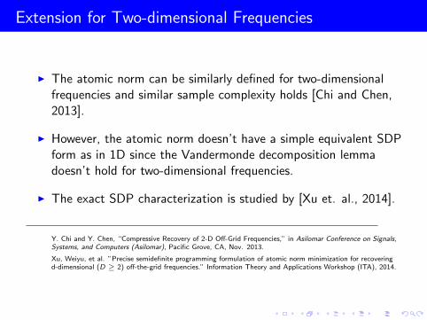
Extension for Two-dimensional Frequencies
I The atomic norm can be similarly defined for two-dimensionalfrequencies and similar sample complexity holds [Chi and Chen,2013].
I However, the atomic norm doesn’t have a simple equivalent SDPform as in 1D since the Vandermonde decomposition lemmadoesn’t hold for two-dimensional frequencies.
I The exact SDP characterization is studied by [Xu et. al., 2014].
Y. Chi and Y. Chen, “Compressive Recovery of 2-D Off-Grid Frequencies,” in Asilomar Conference on Signals,Systems, and Computers (Asilomar), Pacific Grove, CA, Nov. 2013.
Xu, Weiyu, et al. ”Precise semidefinite programming formulation of atomic norm minimization for recoveringd-dimensional (D ≥ 2) off-the-grid frequencies.” Information Theory and Applications Workshop (ITA), 2014.
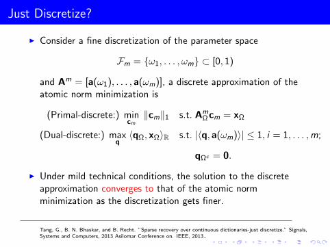
Just Discretize?
I Consider a fine discretization of the parameter space
Fm = ω1, . . . , ωm ⊂ [0, 1)
and Am = [a(ω1), . . . , a(ωm)], a discrete approximation of theatomic norm minimization is
(Primal-discrete:) mincm‖cm‖1 s.t. Am
Ω cm = xΩ
(Dual-discrete:) maxq〈qΩ, xΩ〉R s.t. |〈q, a(ωm)〉| ≤ 1, i = 1, . . . ,m;
qΩc = 0.
I Under mild technical conditions, the solution to the discreteapproximation converges to that of the atomic normminimization as the discretization gets finer.
Tang, G., B. N. Bhaskar, and B. Recht. ”Sparse recovery over continuous dictionaries-just discretize.” Signals,Systems and Computers, 2013 Asilomar Conference on. IEEE, 2013..

Outline
Review of Classical Parameter Estimation
Review of Compressive Sensing
Fundamental Limits of Subsampling on Parameter Estimation
Sensitivity of Basis Mismatch and Heuristic Remedies
Going off the GridAtomic Norm MinimizationEnhanced Matrix Completion
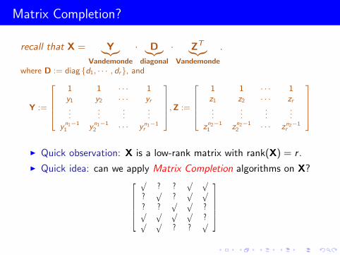
Matrix Completion?
recall that X = Y︸︷︷︸Vandemonde
· D︸︷︷︸diagonal
· ZT︸︷︷︸
Vandemonde
.
where D := diag d1, · · · , dr, and
Y :=
1 1 · · · 1y1 y2 · · · yr...
......
...
yn1−11 yn1−1
2 · · · yn1−1r
,Z :=
1 1 · · · 1z1 z2 · · · zr...
......
...
zn2−11 zn2−1
2 · · · zn2−1r
I Quick observation: X is a low-rank matrix with rank(X) = r .
I Quick idea: can we apply Matrix Completion algorithms on X?
Convex Relaxation
!"""#
!? ?
! !?
!?
! !? ?
! !?! ! ! !?! !
? ?!
$%%%&
' () *!
decompose=
!"""#
!0 0
! !0
!0
! !0 0
! !0! ! ! !0! !
0 0!
$%%%&
' () *!0
+
!"""#
0 ? ? 0 0? 0 ? 0 0? ? 0 0 ?0 0 0 0 ?0 0 ? ? 0
$%%%&
' () *H
• Applying Taylor expansion:
!no = !n
o K!!"#$
sparse matrix
!no + H!
!"#$support known
+ W!"#$residual
– Treat W as noise (BUT WHY???)! W small! H!K!H! and !0 " !n
0 small
Yuxin Chen () Model Selection with Missing Data June 21, 2011 9 / 19

Matrix Completion
I Matrix Completion can be thought as an extension of CS tolow-rank matrices.
I The Netflix problem: Let X ∈ Rn1×n2 satisfying rank(X) = r .
Convex Relaxation
!"""#
!? ?
! !?
!?
! !? ?
! !?! ! ! !?! !
? ?!
$%%%&
' () *!
decompose=
!"""#
!0 0
! !0
!0
! !0 0
! !0! ! ! !0! !
0 0!
$%%%&
' () *!0
+
!"""#
0 ? ? 0 0? 0 ? 0 0? ? 0 0 ?0 0 0 0 ?0 0 ? ? 0
$%%%&
' () *H
• Applying Taylor expansion:
!no = !n
o K!!"#$
sparse matrix
!no + H!
!"#$support known
+ W!"#$residual
– Treat W as noise (BUT WHY???)! W small! H!K!H! and !0 " !n
0 small
Yuxin Chen () Model Selection with Missing Data June 21, 2011 9 / 19
I Given the set of observations PΩ(X), find the matrix with thesmallest rank that satisfies the observations:
minimizeM∈Rn1×n2
rank(M)
subject to PΩ (M) = PΩ (X) ,
users
movies
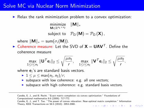
Solve MC via Nuclear Norm Minimization
I Relax the rank minimization problem to a convex optimization:
minimizeM∈Rn1×n2
‖M‖∗
subject to PΩ (M) = PΩ (X) ,
where ‖M‖∗ = sum(σi (M)).I Coherence measure: Let the SVD of X = UΛVT . Define the
coherence measure
max1≤i≤n1
‖UTei‖2 ≤√µn1
r, max
1≤i≤n2
‖VTei‖2 ≤√µn2
r.
where ei ’s are standard basis vectors.I 1 ≤ µ ≤ max(n1, n2)/r ;I subspace with low coherence: e.g. all one vectors;I subspace with high coherence: e.g. standard basis vectors.
Candes, E. J., and B. Recht. ”Exact matrix completion via convex optimization.” Foundations ofComputational mathematics 9.6 (2009): 717-772.Candes, E. J., and T. Tao. ”The power of convex relaxation: Near-optimal matrix completion.” InformationTheory, IEEE Transactions on 56.5 (2010): 2053-2080.

Performance Guarantees and Its Implication
Theorem (Candes and Recht 2009, Gross 2010, Chen 2013)
Assume we collect m = |Ω| samples of X uniformly at random. Letn = maxn1, n2. Then the nuclear norm minimization algorithmrecovers X exactly with high probability if
m > Cµrn log2 n
where C is some universal constant.
I Implication on our problem: Can we apply Matrix Completionalgorithms on the two-dimensional frequency data matrix X?
I Yes, but it yields sub-optimal performance. It requires at leastr maxn1, n2 samples.
I No, X is no longer low-rank if r > min (n1, n2). Note that r canbe as large as n1n2
Candes, E. J., and B. Recht. ”Exact matrix completion via convex optimization.” Foundations ofComputational mathematics 9.6 (2009): 717-772.Gross, David. ”Recovering low-rank matrices from few coefficients in any basis.” Information Theory, IEEETransactions on 57, no. 3 (2011): 1548-1566.Chen, Yudong. ”Incoherence-Optimal Matrix Completion.” arXiv preprint arXiv:1310.0154 (2013).

Revisiting Matrix Pencil: Matrix Enhancement
Given a data matrix X, Hua proposed thefollowing matrix enhancement fortwo-dimensional frequency models:
I Choose two pencil parameters k1 and k2;5 10 15 20 25 30 35
5
10
15
20
25
30
35
I An enhanced form Xe is an k1 × (n1 − k1 + 1) blockHankel matrix :
Xe =
X0 X1 · · · Xn1−k1
X1 X2 · · · Xn1−k1+1
......
......
Xk1−1 Xk1 · · · Xn1−1
,
where each block is a k2 × (n2 − k2 + 1) Hankel matrix asfollows
Xl =
xl,0 xl,1 · · · xl,n2−k2
xl,1 xl,2 · · · xl,n2−k2+1
......
......
xl,k2−1 xl,k2 · · · xl,n2−1
.
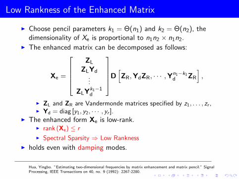
Low Rankness of the Enhanced Matrix
I Choose pencil parameters k1 = Θ(n1) and k2 = Θ(n2), thedimensionality of Xe is proportional to n1n2 × n1n2.
I The enhanced matrix can be decomposed as follows:
Xe =
ZL
ZLYd...
ZLYk1−1d
D
[ZR,YdZR, · · · ,Yn1−k1
d ZR
],
I ZL and ZR are Vandermonde matrices specified by z1, . . . , zr ,I Yd = diag [y1, y2, · · · , yr ].
I The enhanced form Xe is low-rank.I rank (Xe) ≤ r
I Spectral Sparsity ⇒ Low Rankness
I holds even with damping modes.
Hua, Yingbo. ”Estimating two-dimensional frequencies by matrix enhancement and matrix pencil.” SignalProcessing, IEEE Transactions on 40, no. 9 (1992): 2267-2280.

Enhanced Matrix Completion (EMaC)
I The natural algorithm is to find the enhanced matrix with theminimal rank satisfying the measurements:
minimizeM∈Cn1×n2
rank (Me)
subject to Mi ,j = Xi ,j ,∀(i , j) ∈ Ω
where Ω denotes the sampling set.
I Motivated by Matrix Completion, we will solve its convexrelaxation:
(EMaC) : minimizeM∈Cn1×n2
‖Me‖∗subject to Mi ,j = Xi ,j , ∀(i , j) ∈ Ω
where ‖ · ‖∗ denotes the nuclear norm.
I The algorithm is referred to as Enhanced Matrix Completion(EMaC).
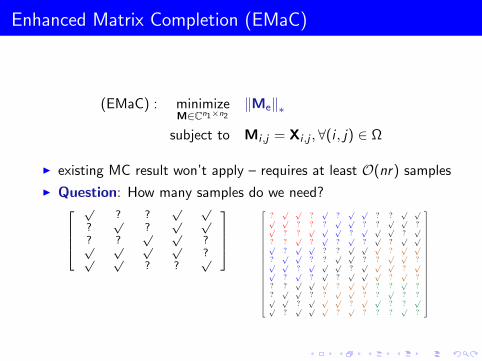
Enhanced Matrix Completion (EMaC)
(EMaC) : minimizeM∈Cn1×n2
‖Me‖∗subject to Mi ,j = Xi ,j ,∀(i , j) ∈ Ω
I existing MC result won’t apply – requires at least O(nr) samples
I Question: How many samples do we need?
Convex Relaxation
!"""#
!? ?
! !?
!?
! !? ?
! !?! ! ! !?! !
? ?!
$%%%&
' () *!
decompose=
!"""#
!0 0
! !0
!0
! !0 0
! !0! ! ! !0! !
0 0!
$%%%&
' () *!0
+
!"""#
0 ? ? 0 0? 0 ? 0 0? ? 0 0 ?0 0 0 0 ?0 0 ? ? 0
$%%%&
' () *H
• Applying Taylor expansion:
!no = !n
o K!!"#$
sparse matrix
!no + H!
!"#$support known
+ W!"#$residual
– Treat W as noise (BUT WHY???)! W small! H!K!H! and !0 " !n
0 small
Yuxin Chen () Model Selection with Missing Data June 21, 2011 9 / 19
?√ √
?√
?√ √
? ?√ √
√ √? ? ?
√ √? ?
√ √?√
? ?√ √ √
?√ √ √
?√
? ?√
?√
?√
?√
?√ √
√?√ √
? ?√ √ √
?√ √
?√ √
? ?√ √
? ?√ √
?√ √?√ √ √
?√ √ √
?√
√?√
?√
?√ √ √
?√
?? ?
√ √ √?√ √
? ?√
??√ √
? ?√ √
? ?√
? ?√ √?√ √ √
?√ √
? ?√
√?√ √ √
?√
? ? ?√
?
Page 15

Introduce Coherence Measure
I Define the 2-D Dirichlet kernel:
K(k1, k2, f1, f2) :=1
k1k2
(1− e−j2πk1f1
1− e−j2πf1
)(1− e−j2πk2f2
1− e−j2πf2
),
I Define GL and GR as r × r Gram matrices such that
(GL)i ,l = K(k1, k2, f1i − f1l , f2i − f2l),
(GR)i ,l = K(n1 − k1 + 1, n2 − k2 + 1, f1i − f1l , f2i − f2l).
separation on x axis
separa
tion o
n y
axis
−0.5 −0.4 −0.3 −0.2 −0.1 0 0.1 0.2 0.3 0.4 0.5
−0.5
−0.4
−0.3
−0.2
−0.1
0
0.1
0.2
0.3
0.4
0.5 0
0.1
0.2
0.3
0.4
0.5
0.6
0.7
0.8
0.9
1

Introduce Coherence Measure
I Incoherence condition holds w.r.t. µ if
σmin (GL) ≥ 1
µ, σmin (GR) ≥ 1
µ.
I µ = Θ(1) holds under many scenarios:I Randomly generated frequencies;I Mild perturbation of grid points;I In 1D, well-separated frequencies by 2 times RL [Liao and
Fannjiang, 2014].
W. Liao and A. Fannjiang. ”MUSIC for Single-Snapshot Spectral Estimation: Stability and Super-resolution.”arXiv preprint arXiv:1404.1484 (2014).

Theoretical Guarantees for Noiseless Case
Theorem (Chen and Chi, 2013)
Let n = n1n2. If all measurements are noiseless, then EMaC recoversX perfectly with high probability if
m > Cµr log3 n.
where C is some universal constant.
I deterministic signal model, random observation;I coherence condition µ only depends on the frequencies but the
amplitudes.I near-optimal within logarithmic factors: Θ(r log3 n).I general theoretical guarantees for Hankel (Toeplitz) matrix
completion, which are useful for applications in control, MRI,natural language processing, etc.
Y. Chen and Y. Chi, “Robust Spectral Compressed Sensing via Structured Matrix Completion,” IEEE Trans. onInformation Theory, Apr. 2013, in revision.

Phase Transition
m: number of samples
r: s
pars
ity level
20 40 60 80 100 120 140 160 180 200
2
4
6
8
10
12
14
16
18
20
22
0
0.1
0.2
0.3
0.4
0.5
0.6
0.7
0.8
0.9
1
Figure : Phase transition diagrams where spike locations are randomlygenerated. The results are shown for the case where n1 = n2 = 15.
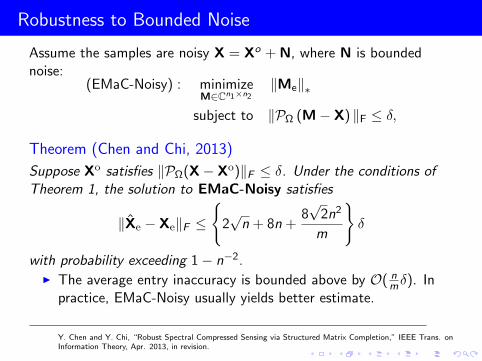
Robustness to Bounded Noise
Assume the samples are noisy X = Xo + N, where N is boundednoise:
(EMaC-Noisy) : minimizeM∈Cn1×n2
‖Me‖∗subject to ‖PΩ (M− X) ‖F ≤ δ,
Theorem (Chen and Chi, 2013)
Suppose Xo satisfies ‖PΩ(X− Xo)‖F ≤ δ. Under the conditions ofTheorem 1, the solution to EMaC-Noisy satisfies
‖Xe − Xe‖F ≤
2√
n + 8n +8√
2n2
m
δ
with probability exceeding 1− n−2.I The average entry inaccuracy is bounded above by O( n
mδ). Inpractice, EMaC-Noisy usually yields better estimate.
Y. Chen and Y. Chi, “Robust Spectral Compressed Sensing via Structured Matrix Completion,” IEEE Trans. onInformation Theory, Apr. 2013, in revision.

Singular Value Thresholding (Noisy Case)
I Several optimized solvers for Hankel matrix completion exist, forexample [Fazel et. al. 2013, Liu and Vandenberghe 2009]
Algorithm 1 Singular Value Thresholding for EMaC
1: initialize Set M0 = Xe and t = 0.2: repeat3: 1) Qt ← Dτt (Mt) (singular-value thresholding)4: 2) Mt ← HankelX0 (Qt) (projection onto a Hankel matrix consistent
with observation)5: 3) t ← t + 16: until convergence
0 10 20 30 40 50 60 70 80 90 1000
5
10
15
20
25
Time (vectorized)
Am
plit
ud
e
True Signal
Reconstructed Signal
Figure : dimension: 101× 101, r = 30, mn1n2
= 5.8%, SNR = 10dB.

Robustness to Sparse Outliers
I What if a constant portion of measurements are arbitrarilycorrupted?
Xcorruptedi ,l = Xi ,l + Si ,l
where Si ,l is of arbitrary amplitude.I Reminiscent of the robust PCA approach [Candes et. al. 2011,
Chandrasekaran et. al. 2011]
I Solve the following algorithm:
(RobustEMaC) : minimizeM,S∈Cn1×n2
‖Me‖∗ + λ‖Se‖1
subject to (M + S)i ,l = Xcorruptedi ,l , ∀(i , l) ∈ Ω
0 10 20 30 40 50 60−8
−6
−4
−2
0
2
4
6
8
data index
rea
l p
art
clean signal
noisy samples

Theoretical Guarantees for Robust Recovery
(RobustEMaC) : minimizeM,S∈Cn1×n2
‖Me‖∗ + λ‖Se‖1
subject to (M + S)i ,l = Xcorruptedi ,l , ∀(i , l) ∈ Ω.
Theorem (Chen and Chi, 2013)
Assume the percent of corrupted entries is s is a small constant. Setn = n1n2 and λ = 1√
m log n. Then RobustEMaC recovers X with high
probability ifm > Cµr 2 log3 n,
where C is some universal constant.
I Sample complexity: m ∼ Θ(r 2 log3 n), slight loss than theprevious case;
I Robust to a constant portion of outliers: s ∼ Θ(1)
Y. Chen and Y. Chi, “Robust Spectral Compressed Sensing via Structured Matrix Completion,” IEEE Trans. onInformation Theory, Apr. 2013, in revision.

Robustness to Sparse Corruptions
0 10 20 30 40 50 60−8
−6
−4
−2
0
2
4
6
8
data index
real part
clean signal
noisy samples
0 10 20 30 40 50 60−8
−6
−4
−2
0
2
4
6
8
data index
real part
clean signal
recovered signal
recovered corruptions
(a) Observation (b) Recovery
Figure : Robustness to sparse corruptions: (a) Clean signal and its corruptedsubsampled samples; (b) recovered signal and the sparse corruptions.

Phase Transition for Line Spectrum Estimation
Fix the amount of corruption as 10% of the total number of samples:
m: number of samples
r: s
pa
rsity le
ve
l
20 40 60 80 100
5
10
15
20
25
0
0.1
0.2
0.3
0.4
0.5
0.6
0.7
0.8
0.9
1
Figure : Phase transition diagrams where spike locations are randomlygenerated. The results are shown for the case where n = 125.

Comparisons between the two Approaches
EMaC Atomic Norm
Signal model Deterministic Random
Observation model Random Random
Success Condition Coherence Separation condition
Amplitudes No condition Randomly generated
Sample Complexity Θ(r log3 n) Θ(r log r log n)
Bounded Noise Yes Not shown
Sparse Corruptions Yes Not shown

Comparisons of EMaC and Atomic Norm Minimization
Phase transition for line spectrum estimation: numerically, theEMaC approach seems less sensitive to the separation condition.
• without separation
• with 1.5 RL separation
EMaC Atomic Norm
m: number of samples
r: s
pars
ity level
20 30 40 50 60 70 80 90 100 110 1200
5
10
15
20
25
30
35
40
0
0.1
0.2
0.3
0.4
0.5
0.6
0.7
0.8
0.9
1
m: number of samples
r: s
pars
ity level
20 30 40 50 60 70 80 90 100 110 1200
5
10
15
20
25
30
35
40
0
0.1
0.2
0.3
0.4
0.5
0.6
0.7
0.8
0.9
1
m: number of samples
r: s
pars
ity level
20 30 40 50 60 70 80 90 100 110 1200
5
10
15
20
25
30
35
40
0
0.1
0.2
0.3
0.4
0.5
0.6
0.7
0.8
0.9
1
m: number of samples
r: s
pars
ity level
20 30 40 50 60 70 80 90 100 110 1200
5
10
15
20
25
30
35
40
0
0.1
0.2
0.3
0.4
0.5
0.6
0.7
0.8
0.9
1
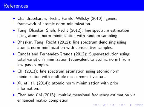
References
I Chandrasekaran, Recht, Parrilo, Willsky (2010): generalframework of atomic norm minimization.
I Tang, Bhaskar, Shah, Recht (2012): line spectrum estimationusing atomic norm minimization with random sampling.
I Bhaskar, Tang, Recht (2012): line spectrum denoising usingatomic norm minimization with consecutive samples.
I Candes and Fernandez-Granda (2012): Super-resolution usingtotal variation minimization (equivalent to atomic norm) fromlow-pass samples.
I Chi (2013): line spectrum estimation using atomic normminimization with multiple measurement vectors.
I Xu et. al. (2014): atomic norm minimization with priorinformation.
I Chen and Chi (2013): multi-dimensional frequency estimation viaenhanced matrix completion.

References
I Xu et. al. (2013): exact SDP characterization of atomic normminimization for high-dimensional frequencies.
I Tang et. al. (2013): near minimax line spectrum denoising viaatomic norm minimization.
I Chi and Chen (2013): higher dimensional spectrum estimationusing atomic norm minimization with random sampling.
I Hua (1992): matrix pencil formulation for multi-dimensionalfrequencies.
I Liao and Fannjiang (2014): analysis of the MUSIC algorithmwith separation conditions.

Concluding Remarks
I Compression, whether by linear maps (e.g, Gaussian) or bysubsampling, has performance consequences for parameterestimtion. Fisher information decreases, CRB increases, and theonset of breakdown threshold increases.
I Model mismatch is inevitable and can result in considerableperformamce degredation, and therefore sensitivities of CS tomodel mismatch need to be fully understood.
I Recent off-the-grid methods provide a way forward for a class ofproblems, where modes to be estimated respect certainseparation or coherence conditions. But sub-Rayleigh resolutionstill eludes us!

Thank You! Questions?