compost land management and soil carbon sequestration

James Madison University James Madison University

JMU Scholarly Commons JMU Scholarly Commons

Senior Honors Projects, 2010-current Honors College

Spring 2016

Compost land management and soil carbon sequestration Compost land management and soil carbon sequestration

Kylene A. Hohman James Madison University

Follow this and additional works at: https://commons.lib.jmu.edu/honors201019

Part of the Agricultural Science Commons, Agronomy and Crop Sciences Commons, Biogeochemistry

Commons, Botany Commons, Environmental Health and Protection Commons, Environmental Monitoring

Commons, Natural Resources and Conservation Commons, Oil, Gas, and Energy Commons, Soil Science

Commons, and the Systems Biology Commons

Recommended Citation Recommended Citation Hohman, Kylene A., "Compost land management and soil carbon sequestration" (2016). Senior Honors Projects, 2010-current. 145. https://commons.lib.jmu.edu/honors201019/145

This Thesis is brought to you for free and open access by the Honors College at JMU Scholarly Commons. It has been accepted for inclusion in Senior Honors Projects, 2010-current by an authorized administrator of JMU Scholarly Commons. For more information, please contact [email protected].

https://commons.lib.jmu.edu/

https://commons.lib.jmu.edu/honors201019

https://commons.lib.jmu.edu/honors

https://commons.lib.jmu.edu/honors201019?utm_source=commons.lib.jmu.edu%2Fhonors201019%2F145&utm_medium=PDF&utm_campaign=PDFCoverPages

http://network.bepress.com/hgg/discipline/1063?utm_source=commons.lib.jmu.edu%2Fhonors201019%2F145&utm_medium=PDF&utm_campaign=PDFCoverPages













https://commons.lib.jmu.edu/honors201019/145?utm_source=commons.lib.jmu.edu%2Fhonors201019%2F145&utm_medium=PDF&utm_campaign=PDFCoverPages

mailto:[email protected]

Compost Land Management and Soil Carbon Sequestration

_______________________

An Honors Program Project Presented to

the Faculty of the Undergraduate

College of Integrated Science and Technology

James Madison University _______________________

by Kylene Hohman

Accepted by the faculty of the Department of Integrated Science and Technology, James Madison University, in partial fulfillment of the requirements for the Honors Program. FACULTY COMMITTEE: Project Advisor: Wayne S. Teel, Ph.D. Professor, GS, ISAT Reader: Jennifer Coffman, Ph.D Associate Professor, ISAT, GS Associate Executive Director, International Programs Reader: Joy Ferenbaugh, Ph.D. Assistant Professor, ISAT

HONORS PROGRAM APPROVAL: Bradley R. Newcomer, Ph.D., Director, Honors Program

PUBLIC PRESENTATION

This work is accepted for presentation, in part or in full, at ISAT Senior Symposium on April 15, 2016.

2

Table of Contents

List of Figures 5

List of Tables 6

Acknowledgements 8

Abstract 9

Chapter 1 Introduction 10

1.1 Existing Dilemma 10

1.2 Counterbalancing the Carbon 11

1.3 Sequestration Procedure 12

1.4 Organic Matter Amendment Proposal 13

1.5 Marin Carbon Project Model 14

1.6 Experimental Design 15

1.7 Research Implications 16

Chapter 2 Literature Review 18

2.1 Marin Carbon Project 18

2.2 Jeffrey Creque Olive Farm 21

2.3 Marin and Sonoma Studies 22

2.4 Marshwind Farm Study 24

Chapter 3 Objectives 26

Chapter 4 Methodology 28

4.1 Study Site Background 28

4.2 Individual Study Plots 28

4.3 Implemented Treatments 29

3

4.4 Composted Plots 30

4.5 Soil Sample Collection 30

4.6 Sample Storage 31

4.7 Sample Conditioning 32

4.8 Muffle Furnace Preparation 33

4.9 Soil Drying and Burning 34

4.10 Soil Carbon Calculation 37

4.11 Carbon Content Visualization 38

4.12 Statistical Analysis 39

Chapter 5 Results 40

5.1 Soil Carbon Content 40

5.2 ArcGIS Visualization of Soil Carbon Content 45

5.3 Statistical Analysis Between Treatments 49

5.4 Waypoint Analytical Soil Characteristics 52

5.5 Statistical Analysis of Waypoint Data Between Treatments 56

Chapter 6 Discussion 58

6.1 Soil Carbon Content Interpretation 58

6.2 Statistical Analysis Interpretation 63

6.2.1 Replication One 63

6.2.2 Replication Two 65

6.2.3 Replication Three 66

6.2.4 Replication Four 68

6.2.5 Time Restraint 69

4

6.3 Waypoint Analytical Soil Characteristics Interpretation 70

6.4 Waypoint Analytical Statistical Analysis Interpretation 74

6.4.1 Organic Matter Percentage 74

6.4.2 Cation Exchange Capacity 75

6.4.3 Phosphorous Concentration 77

6.5 Data Omitted 79

Chapter 7 Conclusion 81

Chapter 8 Future Work 86

Chapter 9 Unintended Consequences 91

Bibliography 93

5

List of Figures

Figure 1 Geographic Coordinate Location of Soil Samples in ArcGIS 31

Figure 2 CSC Scientific Sieve Shaker 33

Figure 3 Desiccant Chamber Storing Sample Crucibles 34

Figure 4 Muffle Furnace Used for Drying and Burning Samples 35

Figure 5 Soil Samples Prior to Drying Procedure 36

Figure 6 Soil Samples Following Drying Procedure 36

Figure 7 Soil Samples Following Drying Procedure 37

Figure 8 Replication One Soil Carbon Content Visualization in ArcGIS 46

Figure 9 Replication Two Soil Carbon Content Visualization in ArcGIS 47

Figure 10 Replication Three Soil Carbon Content Visualization in ArcGIS 48

Figure 11 Replication Four Soil Carbon Content Visualization in ArcGIS 49

6

List of Tables

Table 1 Soil Sample Location and Characteristic Data 29

Table 2 Replication One Soil Carbon Content 41

Table 3 Replication Two Soil Carbon Content 42

Table 4 Replication Three Soil Carbon Content 43

Table 5 Replication Four Soil Carbon Content 44

Table 6 Average Soil Carbon Content Across All Replications 45

Table 7 Replication One Statistical Analysis Between Treatments 51

Table 8 Replication Two Statistical Analysis Between Treatments 51

Table 9 Replication Three Statistical Analysis Between Treatments 51

Table 10 Replication Four Statistical Analysis Between Treatments 52

Table 11 Soil Sample Organic Matter Percentages Obtained from Waypoint Laboratory 53

Table 12 Soil Sample Cation Exchange Capacity Obtained from Waypoint Laboratory 54

Table 13 Soil Sample Phosphorous Content Obtained from Waypoint Laboratory 55

Table 14 Average Soil Characteristic Data Obtained from Waypoint Laboratory 56

Table 15 Statistical Analysis between Treatments of Carbon Percentages from Waypoint

Laboratory 57

7

Table 16 Statistical Analysis between Treatments of Cation Exchange Capacity from Waypoint

Laboratory 57

Table 17 Statistical Analysis between Treatments of Phosphorous Content from Waypoint

Laboratory 57

8

Acknowledgments

This project was made possible by the collaboration and effort of multiple individuals. I wish to

express my sincerest appreciation to Dr. Wayne Teel, whose dedication and support made this

capstone research project possible. Dr. Teel’s continuous commitment and guidance functioned

as the foundation for this project, and this project’s success would not have been feasible without

him. I would also like to extend my gratitude towards Dr. MeiMei Lin, who was as a crucial

collaborator in this project. Dr. Lin extended her time and expertise by formulating the ArcGIS

images utilized as a means of data visualization in this project. Dr. Jennifer Coffman and Dr. Joy

Ferenbaugh, my thesis readers for this capstone project, greatly assisted me in the data collection

process of this experiment. Additionally, Dr. Coffman and Dr. Ferenbaugh have both served as a

valuable resources through the duration of this experiment. I would also like to acknowledge Dr.

Robert Brent, who graciously contributed his time and assistance in preparing my thesis

presentation. I am also grateful for the guidance Kyle Snow provided in the laboratory used

when executing measurements in this experiment. Mr. Snow shared his proficiency in operating

the lab equipment necessary for the completion of this thesis project. I would also like to thank

Fred Garst with the United States Department of Agriculture for offering his time and expertise

as a GIS specialist. Lastly, I would like to extent my dearest gratitude towards the ISAT

Department and Honors Program for offering endless means of support and direction throughout

my JMU career.

9

Abstract

Extensive fossil fuel burning has released carbon dioxide into the atmosphere. Under proper

ecological conditions plants convert atmospheric carbon dioxide into stable soil organic matter, a

natural and efficient means of mitigating climate change. In the symbiotic relationship between

mycorrhizae and plants, mycorrhizae provide plants with essential nutrients in exchange for

carbon sugars leaked from the plants. Mycorrhizae convert carbon sugars to an exudate called

glomalin, a protein that assists in developing soil aggregates composed of sand, silt, and clay.

These aggregates, called humus, store carbon for hundreds of years under healthy ecological

conditions. Compost prompts soil microbes to aerobically transform organic matter into nutrients

readily available to plants. Compost fosters the relationship between plants, mycorrhizae, and

soil organisms to enrich the humification process. The Marin Carbon Project is an effort to

augment this soil carbon sequestration process through compost application onto California

rangelands. This project is being modeled on the East Campus Hillside to determine if compost

boosts carbon storage within soils. The Hillside area has 1.5 acres of a tallgrass prairie. Eight 10

x 10 meter prairie plots were treated with compost, another eight prairie area plots served as

controls, and the remaining 6 plots were located in the lawn area for comparison. Soil samples

were gathered from each plot by the ISAT 320 class and analyzed by the Waypoint Laboratory.

Additional samples were collected and then burned in an on-campus muffle furnace to calculate

the total carbon from each sample. The data assembled from the muffle furnace was analyzed

spatially and statistically to investigate correlations between the soil treatment and percentage of

stable soil carbon. Across the replications executed, soil treated with compost had the highest

carbon percentage. Results from this experiment will be integrated into the ongoing study of the

health of the East Campus Hillside.

10

Chapter 1 Introduction

1.1 Existing Dilemma

In 2013, scientists calculated that the concentration of carbon dioxide present within the

atmosphere had risen to a level of 400 parts per million (ppm) for the first time in over five

million years [1, p. XVIII]. It has been estimated that to maintain a stable atmosphere suitable for

human life, the concentration of carbon dioxide within the atmosphere must remain below 350

ppm [2, p. 16]. Although carbon dioxide occurs naturally in the atmosphere and is essential for

keeping the Earth at a suitable temperature for human life, the sources of rising carbon dioxide

emissions are largely anthropogenic. In 2014, the Environmental Protection Agency (EPA)

calculated that 80.9% of the entire U.S. greenhouse gas emissions being emitted by human

actions were carbon dioxide [3]. Human activities have effectively altered the carbon cycle by

pumping more emissions into the atmosphere and by altering stable reservoirs, such as the

atmosphere, oceans, soils, and forests [3]. Fossil fuel usage has surged the amount of carbon

dioxide emissions being pumped into the atmosphere. Fossil fuels such as coal, natural gas, and

oil are utilized for electricity, transportation, and industry. In 2014, combustion of fossil fuels to

produce electricity accounted for 37% of all U.S. carbon dioxide emissions, and 30% of all the

greenhouse gas emissions within the United States [3]. Usage of fossil fuels such as gasoline and

diesel for transportation generated 31% of all the U.S. carbon dioxide emissions and 25% of the

total U.S. greenhouse gas emissions in 2014 [3]. Industry accounts for the third largest source of

carbon dioxide emissions in the United States. Industries utilize fossil fuel combustion for energy

and emit carbon dioxide through chemical manufacturing processes. In the United States, carbon

dioxide emissions from industries accounted for 15% of all U.S. carbon dioxide emissions and

12% of all U.S. greenhouse gas emissions in 2014 [3]. Aside from a direct increase in carbon

11

dioxide emissions, land use and land cover change have also accounted for an alteration in the

carbon cycle. As land is cleared during deforestation, densely packed plants and trees are

cleared. These living organisms possess the capability to cycle large amounts of carbon through

photosynthesis, and thus harbor a large quantity of carbon. Removing vegetation eradicates an

effective means of naturally offsetting carbon dioxide emissions and thus an essential step in the

carbon cycle. Greenhouse gas emissions such as carbon dioxide absorb energy and can either

decelerate or half the loss of heat to space [4], which effectively warms the Earth. This destructive

cycle of altering the carbon cycle and boosting emissions has threatened the capability to sustain

future generations due to the treat of climate change.

1.2 Counterbalancing the Carbon

The Earth has previously cycled this carbon effectively by absorbing it into its natural

sinks – the atmosphere, oceans, forests, and soils. Because carbon dioxide is being pumped into

the atmosphere from anthropogenic sources at unsustainable rates, some of these reservoirs do

not currently possess the capacity to effectively store carbon dioxide. As many of these

emissions are released directly into the atmosphere, scientists have deemed the atmosphere to be

“full” of carbon dioxide and thus unable to continue storing these emissions [1, p. 6]. Scientists

have also warned that the oceans are slowly “filling up” and in a few decades will be saturated

with carbon to an extent at which it can no longer store these emissions [1, p. 6]. Forests, which can

stably store carbon is managed properly, are currently being stripped from the Earth or

improperly managed. As forests are burned and trees die, the carbon dioxide is immediately

released directly into the atmosphere again [1, p. 6]. The last carbon sink, soil, has been depleted of

its carbon stocks and thus can serve as an effective means of harboring carbon. Due to ongoing

cultivation occurring for millennia, up to 80% of soil carbon has been depleted [2, p. 15]. Poor soil

12

management has released the carbon stored within the soil, accounting for a loss of up to 80

billion tons of carbon from the soil [2, p. 15]. Examples of poor soil management include tillage,

chemical fertilizer application, overgrazing, monoculture farms, and poor perennial crop

management. Because soils have been depleted of their carbon, they are available to soak up the

excess carbon dioxide currently lodged in the atmosphere. Through effective land management

techniques, the organic matter content of soils can be boosted to create a reservoir available for

uptake of atmospheric carbon dioxide. Research has predicted that a 2% increase in the organic

content of the planet’s soils could absorb all the excess atmospheric carbon dioxide within a

decade [1, p. 7].

1.3 Sequestration Procedure

The process of extracting atmospheric carbon dioxide naturally and storing it in the soil

stably for an extended period of time is termed sequestration. Carbon sequestration is composed

largely of four main steps that include photosynthesis, resynthesis, exudation, and humification

[1, p. 19]. In the photosynthesis step, plants utilize sunlight energy as a means to break apart water

molecules into their hydrogen and oxygen components. The oxygen is released directly back into

the atmosphere and during the second stage of photosynthesis the hydrogen atoms are bound to

carbon dioxide molecules from the atmosphere. When the hydrogen molecules are combined

with the carbon dioxide molecules, a simple carbohydrate called glucose is created. In the

second, resynthesis, the glucose previously formulated is resynthesized into numerous carbon

compounds by means of a sequence of complex chemical reactions. In the third step of

sequestration, 30 to 40 percent [1, p. 19] of the carbon synthesized during photosynthesis is directly

released into the soil through the plant roots. This leaked carbon is called liquid carbon or root

exudates. When the carbon is expelled into the soil, it nurtures the soil microbes that assist in

13

building topsoil. As these microbes such as bacteria and fungi consume the leaked carbon, they

provide the plant with nutrients in exchange. These nutrients, such as phosphorus and nitrogen,

were not otherwise available to these plants and thus an essential symbiotic relationship between

the soil microbes and plants is formed. As this relationship expands, mycorrhizal fungi begin to

colonize the roots of their host plant to assist in connecting the plant to the surrounding

environment through hyphae [1, p. 19]. Enabling this fungal colonization of plant roots enhances

the plants ability to uptake water and mineral nutrients. The final step of sequestration involves

the humification process. Humus is a chemically stable form of organic matter [1, p. 19]. Carbon

storage as humus is highly resistant against decomposition and is capable of remaining within the

soil for hundreds of years [1, p. 19] under proper land management practices. After the mycorrhizal

fungi utilize the expelled carbon, they expel a protein called glomalin. This glycoprotein binds

soil aggregates together that consist of sand, silt, and clay particles. The formation of these soil

aggregates enhances the amount of stable soil carbon called humus.

1.4 Organic Matter Amendment Proposal

Organic matter amendments to the soil have been recommended as a means to increase

carbon storage within soils [5]. The implications of this organic matter amendment are both direct

and indirect. An organic matter amendment directly inputs carbon into the soil from the

amendment itself, and an increase in carbon storage within soils also occurs indirectly from

boosted plant production [6]. An effective land management technique that has been proposed is a

compost application. Soil microbes are capable of effectively converting the organic matter

present within compost into nutrients readily available for plants. The boost in organic matter

thus fosters the relationship between actively growing plants and the soil microbes that assist in

building the topsoil. Because composted materials are already partially decomposed, the organic

14

matter incorporated into the soil through compost application tends to be more resilient with a

higher carbon ratio than an application of fresh plant litter or animal manures [7]. While some of

the added organic matter from compost is rapidly decomposed by soil microbes, a portion of the

organic matter is merged into soil aggregates, which physically and biochemically shields the

organic matter from decomposition [7]. Because the organic matter is protected from

decomposition, these carbon pools will remain within the soil for decades before turning over [7].

Compost can thus serve as a slow release natural fertilizer for plants and soils, enhancing the

carbon sequestration process and plant production. With enhanced plant production occurring in

soils, more liquid carbon can be leaked into the soil, leading to a boosted humification process

and amount of carbon stored.

1.5 Marin Carbon Project Model

This research is being modeled after the Marin Carbon Project, which is currently an

ongoing experiment that is taking place in Nicasio, Marin County, California. John Wick and

Peggy Rathmann initiated this project in 2008, and are currently maintaining its continuation and

dispersion to other testing sites. Peggy and John are working with lead scientist Whendee Silver,

a biogeochemist and professor of ecosystem ecology at the University of California-Berkeley. In

this collaborative study, the effects of an organic matter amendment consisting of composted

green waste are being studied. The researchers hypothesized that the addition of compost would

boost the aboveground and belowground net primary productivity for at least one year [8]. The

hypothesis was tested using replicated field experiments over a period of three years in two

dominant annual grassland types present in California. This particular experiment under the

Marin Carbon Project was executed over three growing seasons starting in October of 2008 [8].

This study involved untreated control plots and plots with a single ½ inch composted organic

15

matter amendment. To prevent unintended negative impacts on forage growth, compost depth

was consistently kept at a depth of ½ inch [9]. A buffer strip of 5 meters separated each 25 x 60 m

in this study, and the plots were arranged into three randomized blocks to reduce bias [8]. After

three years, researchers found that the single compost amendment increased the forage

production by 50% and the soil carbon sequestration by 1 ton/hectare [10]. Research indicated that

the compost application also boosted the net ecosystem carbon storage by 25-70% in the

grasslands [10]. Researchers found that their results agreed with their stated hypothesis that the net

primary productivity would be boosted; as they found that the production of grass on the

composted plots was doubled [10]. From this study, it was concluded that if 1 Mg C ha-1 y-1 was

sequestered on half of the available rangeland area in California, then 42 million metric tons of

carbon dioxide emissions could be offset, which is corresponds to the yearly greenhouse gas

emissions emitted for commercial and residential energy resources in California [10].

1.6 Experimental Design

This research experiment was conducted on a 1.5-acre prairie on the ISAT Hillside at the

James Madison University campus in Harrisonburg, Virginia. The study site was originally

planted with grasses foreign to the landscape but as part of the ISAT Hillside Naturalization

Project, the hillside is now composed of native grasses and wildflower species. The purpose of

the ISAT Hillside Naturalization Project is to successfully convert a monoculture grassland into

a polyculture, carbon sequestering natural prairie. Within the 1.5-acre prairie, 22 10 x 10 meter

plots were devised for the ISAT 320 lab. The plots were measured and marked by students

within the ISAT 320 Fall 2015 class, and these plots served as the testing sites for this

experiment. Eight of the 10 x 10 meter plots located in the prairie were randomly selected to

receive a single half-inch compost amendment in March of 2015. Eight separate 10 x 10 meter

16

plots in the prairie did not receive an organic matter amendment, and thus these plots served as

the control in this study. There were six 10 x 10 meter plots located outside of the prairie in the

lawn area that were also incorporated into this study to serve as a comparison for the prairie

plots. About six months following the single compost application, soil samples were collected

from each of the 22 study locations. Students within the Fall 2015 ISAT 320 Lab also collected

their own individual samples for testing at a separate facility. The samples collected for the

purpose of this experiment were tested on-campus within the JMU Environmental Lab by using a

muffle-furnace and scale. By using a muffle furnace to dry and burn each soil sample, the

weights before and after burning were compared to determine the percentage or organic matter

burned from each sample (Eq. 1). Because carbon is estimated to compose about 45% of organic

matter, this percentage was used to then find the estimated amount of carbon burned from each

sample (Eq. 2). This procedure was executed for a total of four replications to account for

variability within the soil samples and uncertainty introduced within measurements.

1.7 Research Implications

By following the procedure utilized for the Marin Carbon Project, the purpose of this

experiment was to determine if a singular amendment of composted green waste could assist in

boosting the sequestration of carbon within the soil. Findings of boosted carbon sequestration

within the study site would indicate that carbon dioxide atmospheric emissions were successfully

being offset through a natural and cost-effective procedure. With a successfully augmented

carbon sequestration process implemented into the ISAT Hillside, a portion of carbon dioxide

emissions present in the atmosphere from energy expenditures can be offset. This enhanced

release of carbon into the soil through plant roots not only would reduce emissions lingering in

the atmosphere, but it would also boost overall soil and vegetation health. Widespread usage of

17

this procedure would thus possess the power to effectively diminish the negative implications of

amplified greenhouse gas emissions, such as climate change. Rather than relying on expensive

technologies to remove carbon dioxide emissions from the atmosphere, an effective compost

land management technique would serve as a real-world solution that can be applied globally at a

fast rate but low cost.

18

Chapter 2 Literature Review

2.1 Marin Carbon Project

The primary study evaluated for this study was the ongoing Marin Carbon Project

experiment. The main objective of the Marin Carbon Project was to “explore the value of local

soil carbon sequestration in rangelands” [1, p. 10] in an attempt to benefit rural communities both

ecologically and agriculturally. To facilitate the uptake of carbon dioxide, researcher Whendee

Silver spread ½ inch of compost onto pastureland plots [1, p. 11]. The compost utilized within the

Marin Carbon Project was a mixture of plant clippings and animal manure [1, p. 11], a common

compost solution. Silver clarified that the compost intensifies plant growth while also lower the

soil temperature to a degree that doesn’t stimulate heavy microbial activity, which would

subsequently result in active microbes exhaling carbon dioxide back into the atmosphere [1, p. 11].

Visibly, Silver has found that the composted plots portray taller grass, meaning that the grass has

a greater amount of carbon stowed within it [1, p. 11]. Silver has also calculated that the composted

plots within the study successfully seize 50 percent more carbon from the atmosphere than the

grass in the control plots [1, p. 11]. It is estimated by Silver that the compost land management

technique of offsetting carbon dioxide emissions within the atmosphere could be continued for

30 years before the soil became saturated with carbon [1, p. 11].

As part of the Marin Carbon Project, Whendee Silver and Rebecca Ryals conducted a

field experiment on valley grasslands at the Sierra Foothill Research and Extension Center in

Browns Valley, California [8]. The research project was also operated on coastal grasslands in

Nicasio, California [8]. The experiment was established in October of 2008 and was performed

until August of 2011[8]. The plot sizes were 25 x 60 m, and treatments consisted of composted

19

organic matter and untreated control plots[8]. The organic amendment consisted of commercially

available composted green waste, and the soil amendment was applied in December of 2008 [8].

The sites in this study have historically been grazed by cattle since 1900, and thus all plots in the

study were grazed using a rotational system[8]. Calculation of the soil carbon content was

executed prior to and following the organic matter amendment, which would have served as a

useful step in the procedure of this hillside experiment. Soil samples in this study were collected

using a 7 cm corer, and the sample depth was approximately 10 cm [8]. This study also collected

nine separate samples from each plot to analyze spatial differences. To condition the soil sample,

identifiable root and compost pieces were manually removed from the soil samples. To calculate

the carbon content, a Carlo Erba Elantech elemental analyzer was used with an atropine being

utilized as a standard that was altered to content using bulk density values for each plot [8]. To

analyze the data statistically, a one-way analyses of variance (ANOVA) was implemented to find

statistical significant in the soil carbon content between treatments [8].

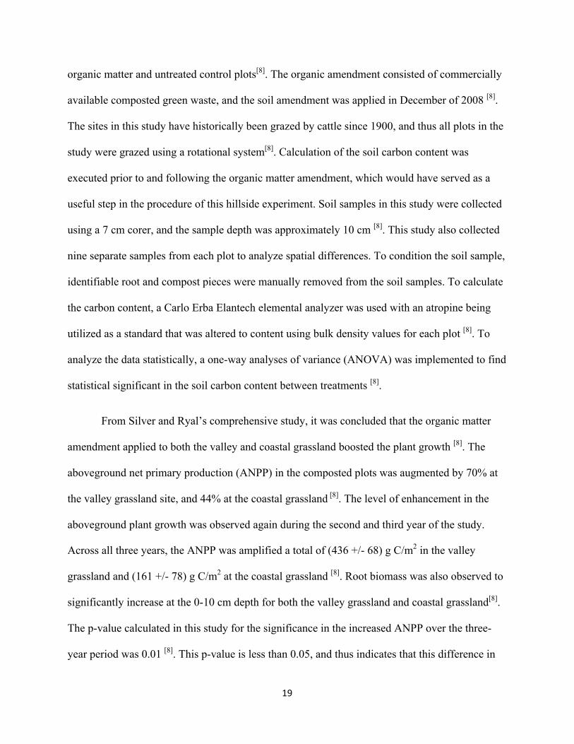
From Silver and Ryal’s comprehensive study, it was concluded that the organic matter

amendment applied to both the valley and coastal grassland boosted the plant growth [8]. The

aboveground net primary production (ANPP) in the composted plots was augmented by 70% at

the valley grassland site, and 44% at the coastal grassland [8]. The level of enhancement in the

aboveground plant growth was observed again during the second and third year of the study.

Across all three years, the ANPP was amplified a total of (436 +/- 68) g C/m2 in the valley

grassland and (161 +/- 78) g C/m2 at the coastal grassland [8]. Root biomass was also observed to

significantly increase at the 0-10 cm depth for both the valley grassland and coastal grassland[8].

The p-value calculated in this study for the significance in the increased ANPP over the three-

year period was 0.01 [8]. This p-value is less than 0.05, and thus indicates that this difference in

20

aboveground plant growth between the compost amended plots and control plots was statistically

significant.

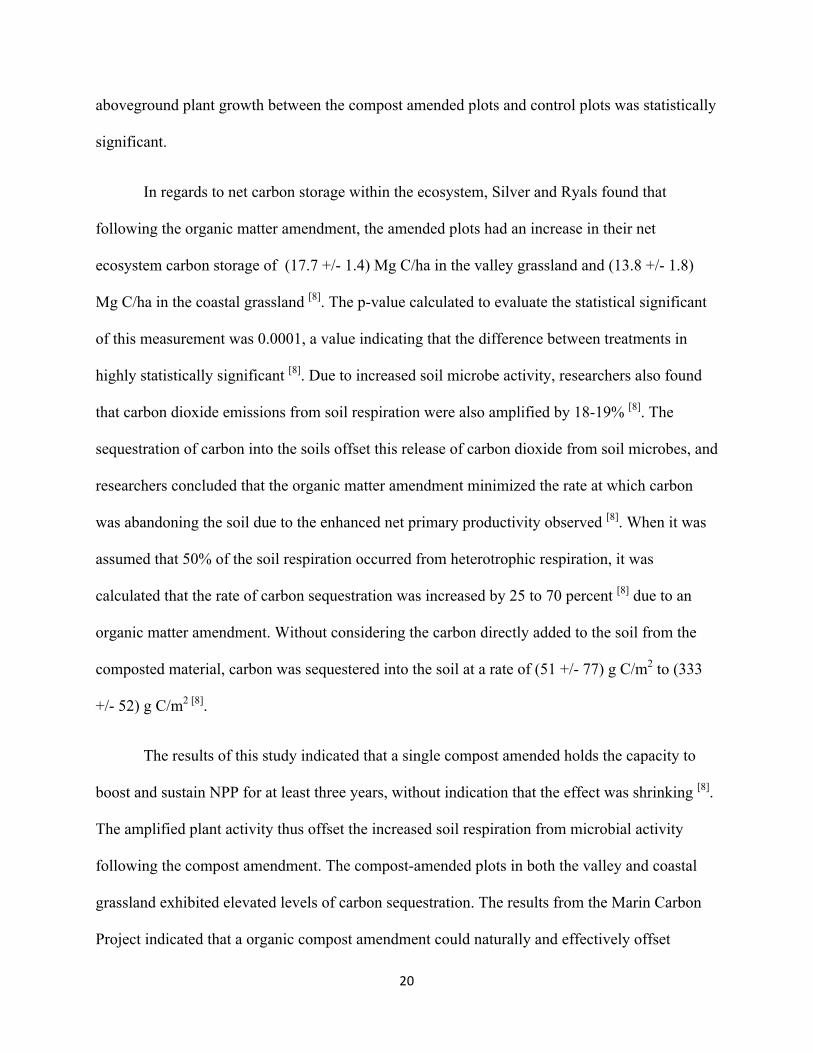
In regards to net carbon storage within the ecosystem, Silver and Ryals found that

following the organic matter amendment, the amended plots had an increase in their net

ecosystem carbon storage of (17.7 +/- 1.4) Mg C/ha in the valley grassland and (13.8 +/- 1.8)

Mg C/ha in the coastal grassland [8]. The p-value calculated to evaluate the statistical significant

of this measurement was 0.0001, a value indicating that the difference between treatments in

highly statistically significant [8]. Due to increased soil microbe activity, researchers also found

that carbon dioxide emissions from soil respiration were also amplified by 18-19% [8]. The

sequestration of carbon into the soils offset this release of carbon dioxide from soil microbes, and

researchers concluded that the organic matter amendment minimized the rate at which carbon

was abandoning the soil due to the enhanced net primary productivity observed [8]. When it was

assumed that 50% of the soil respiration occurred from heterotrophic respiration, it was

calculated that the rate of carbon sequestration was increased by 25 to 70 percent [8] due to an

organic matter amendment. Without considering the carbon directly added to the soil from the

composted material, carbon was sequestered into the soil at a rate of (51 +/- 77) g C/m2 to (333

+/- 52) g C/m2 [8].

The results of this study indicated that a single compost amended holds the capacity to

boost and sustain NPP for at least three years, without indication that the effect was shrinking [8].

The amplified plant activity thus offset the increased soil respiration from microbial activity

following the compost amendment. The compost-amended plots in both the valley and coastal

grassland exhibited elevated levels of carbon sequestration. The results from the Marin Carbon

Project indicated that a organic compost amendment could naturally and effectively offset

21

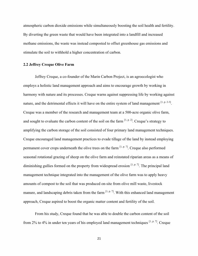
atmospheric carbon dioxide emissions while simultaneously boosting the soil health and fertility.

By diverting the green waste that would have been integrated into a landfill and increased

methane emissions, the waste was instead composted to offset greenhouse gas emissions and

stimulate the soil to withhold a higher concentration of carbon.

2.2 Jeffrey Creque Olive Farm

Jeffrey Creque, a co-founder of the Marin Carbon Project, is an agroecologist who

employs a holistic land management approach and aims to encourage growth by working in

harmony with nature and its processes. Creque warns against suppressing life by working against

nature, and the detrimental effects it will have on the entire system of land management [1, p. 2-3].

Creque was a member of the research and management team at a 500-acre organic olive farm,

and sought to evaluate the carbon content of the soil on the farm [1, p. 2]. Creque’s strategy to

amplifying the carbon storage of the soil consisted of four primary land management techniques.

Creque encouraged land management practices to evade tillage of the land by instead employing

permanent cover crops underneath the olive trees on the farm [1, p. 7]. Creque also performed

seasonal rotational grazing of sheep on the olive farm and reinstated riparian areas as a means of

diminishing gullies formed on the property from widespread erosion [1, p. 7]. The principal land

management technique integrated into the management of the olive farm was to apply heavy

amounts of compost to the soil that was produced on-site from olive mill waste, livestock

manure, and landscaping debris taken from the farm [1, p. 7]. With this enhanced land management

approach, Creque aspired to boost the organic matter content and fertility of the soil.

From his study, Creque found that he was able to double the carbon content of the soil

from 2% to 4% in under ten years of his employed land management techniques [1, p. 7]. Creque

22

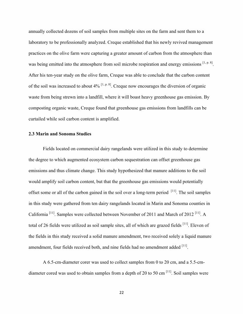
annually collected dozens of soil samples from multiple sites on the farm and sent them to a

laboratory to be professionally analyzed. Creque established that his newly revived management

practices on the olive farm were capturing a greater amount of carbon from the atmosphere than

was being emitted into the atmosphere from soil microbe respiration and energy emissions [1, p. 8].

After his ten-year study on the olive farm, Creque was able to conclude that the carbon content

of the soil was increased to about 4% [1, p. 8]. Creque now encourages the diversion of organic

waste from being strewn into a landfill, where it will boast heavy greenhouse gas emission. By

composting organic waste, Creque found that greenhouse gas emissions from landfills can be

curtailed while soil carbon content is amplified.

2.3 Marin and Sonoma Studies

Fields located on commercial dairy rangelands were utilized in this study to determine

the degree to which augmented ecosystem carbon sequestration can offset greenhouse gas

emissions and thus climate change. This study hypothesized that manure additions to the soil

would amplify soil carbon content, but that the greenhouse gas emissions would potentially

offset some or all of the carbon gained in the soil over a long-term period [11]. The soil samples

in this study were gathered from ten dairy rangelands located in Marin and Sonoma counties in

California [11]. Samples were collected between November of 2011 and March of 2012 [11]. A

total of 26 fields were utilized as soil sample sites, all of which are grazed fields [11]. Eleven of

the fields in this study received a solid manure amendment, two received solely a liquid manure

amendment, four fields received both, and nine fields had no amendment added [11].

A 6.5-cm-diameter corer was used to collect samples from 0 to 20 cm, and a 5.5-cm-

diameter cored was used to obtain samples from a depth of 20 to 50 cm [11]. Soil samples were

23

passed through a 2-mm sieve in this study while visible root and plant fragments were manually

removed [11]. The rocks separated from the soil samples were weighted to determine the rock

concentration of the samples being analyzed. Prior to analyzing the soil samples, they were

ground to a find powder after being dried [11]. A Carlo Erba Elantech elemental analyzer with an

atropine standard was used to calculate the carbon content of the samples being analyzed [11]. To

analyze statistical significance in this study, means were compared with analysis of means

(ANOM) and a statistically significant difference was defined as having a p-value less than 0.10

[11].

From the field measurements, researchers found that there was variation in the soil

carbon concentration within and between the dairies in this study. Overall, researchers found that

the organic matter amendment consisting of manure increased the average soil carbon

concentration by (1.07 +/- 0.81) percent carbon within the 5 to 10 cm soil depth [11]. At an

increased depth of 10 to 20 cm, the average carbon content of the soil increased by (0.88 +/-

0.68) percent carbon in the sites that received an organic matter amendment [11]. At a soil depth

of 0 to 5 cm, the difference in carbon content between the sites that received an organic matter

amendment and the sites that served as controls was not statistically significant [11]. Researchers

concluded that in the top 20 cm of the soil profile, fields with an organic matter amendment had

higher soil carbon content average by (19.0 +/- 7.3) Mg C ha-1 [11].

Researchers from this study predicted that given a longer period of time following the

organic matter amendment to the soil, the soil carbon content would increase at all soil depths

analyzed in this study [11]. Due to high variation within the data collected, the differences in

average carbon content of the soil across treatments could not be concluded to be statistically

significant [11]. It was still concluded from this study that organic matter amendments to

24

rangelands offer the potential to mitigate climate change by offsetting the concentration of

carbon dioxide within the atmosphere. Long-term impacts of an organic matter amendment

suggest that carbon concentration of the soil will continually rise as time elapses. Researchers

predicted that the carbon pools in the soil analyzed would stabilize over time and factors such as

quality, quantity, and time of the organic matter amendment must be optimized such that the

amount of carbon sequestration can be maximized [11].

2.4 Marshwind Farm Study

A field study was conducted on Marshwind Farm, Masstown from 1998 to 2001 to

determine the benefits that composted material can have on a pasture in terms of its soil physical

properties and soil organic matter [12]. Treatments in this study consisted of compost derived

from crop residue, dairy manure, sewage sludge, or liquid dairy manure [12]. An unfertilized

control was also included in this study as a means of comparison for the amended plots. The

mineral fertilizer treatments in this study were applied on an annual basis, but the organic matter

amendments were solely applied in 1998 and 1999 [12]. Soil samples were collected in October of

2000 and 2001 using a split core sampler [12]. Ten samples were collected from each plot, and the

samples collected included the top 15 cm of the soil profile [12]. A sieve was used to remove

gravel, crowns, and large root pieces while any remaining visible root pieces were removed from

the soil samples by hand [12]. To analyze the carbon content of the collected soil, the Dumas

method of direct combustion was implemented into the procedure [12]. Analyzing the statistical

significance of differences between treatments was conducted using the General Linear Model of

SAS software [12].

25

The composted plots in this study significantly boosted the soil carbon sequestration and

mass per volume [12]. This trend of boosted soil carbon sequestration was observed two years

following the final application of composted materials [12]. The compost amendment enhanced

soil organic carbon from 29.3 g C kg-1 in the unfertilized control to 41.5-53.2 g C kg-1 in the

amended soil plots [12]. Researchers reported that compost alone altered the soil organic carbon

and mass by 5.2 to 9.7 Mg C ha-1 [12]. The amendments with lower carbon inputs, such as

manure, reflected a lower gain in soil organic carbon in comparison to the composted material

[12]. Because these treatments were applied to two different crop types, the crop types were found

to respond differently to the soil amendments. This was an element excluded in the hillside

experiment, but it is recommended that future work include specific plant types and densities.

This experiment demonstrated the overall trend that composted amendments applied to

landscapes can boost the total carbon storage in the soil more efficiently than non-composted

materials, yet both enhanced the soil quality by directly providing the soil with organic matter.

Increased carbon storage was observed across all treatments, although the composted materials

augmented carbon sequestration most dramatically. Researchers determined that composts can

be matched to specific crops to provide the greatest results in increased soil fertility and organic

matter content [12]. While this study focused on targeting specific crops with particular types of

organic matter amendments, the conclusion that composted organic materials promote soil

carbon improvements was deducted from the gathered field results [12].

26

Chapter 3 Objectives

The main objective of this experiment was to determine if a singular composted organic

matter amendment could effectively increase the amount of carbon sequestered within the soil.

The goal of this project was to replicate the Marin Carbon Project as closely as possible on the

ISAT Hillside to investigate if the same results would be obtained. Because this was the first

year this experiment was conducted on the ISAT Hillside, a sub-objective of this project was to

develop an operational protocol to foster the successful continuation of this project. This

experiment also aligns with the ISAT Hillside Naturalization Project, which is an ongoing

project with the goal of nurturing the growth of a polyculture wildflower prairie. An area of

study within this experiment was thus to determine if a monoculture grassland could be

converted into a polyculture carbon-sequestering prairie. Lawn plots were incorporated into this

study to serve as a comparison between the prairie plots and the grassland area. Integration of the

grassland into this study will serve to further the research of the ISAT Hillside Naturalization

Project such that it can be concluded if the health of the prairie surpasses the lawn health in

regards to carbon content.

While this project aligned with the Marin Carbon Project, it was still investigative in

nature. The project was not being built upon a previous project conducted on the ISAT Hillside

and was instead the initiation of an ongoing study that will continue to be executed. The

hypothesis of this study was that the plots that received a single compost amendment would have

a higher content of soil carbon compared to the control prairie plots and the lawn plots. This

project established a baseline for understanding the carbon content of the ISAT Hillside soil, as

this data was not recorded prior to the study. By completing this study, it was expected that

differences in soil carbon content would be observable between composted prairie plots, control

27

prairie plots, and lawn plots. This was also the first composted organic matter amendment added

onto the ISAT Hillside for a experimental study, meaning the project was entirely investigative.

Due to climate and soil differences between this experimental study site and the location of the

Marin Carbon Project, it was predicted that while the same trend in carbon content could be

observed, the differences between treatments would vary between the two study sites.

28

Chapter 4 Methodology

4.1 Study Site Background

The study was conducted on a 1.5-acre grass prairie on the ISAT Hillside on the James

Madison University campus in Harrisonburg, Virginia (-78.935, 38.4553) [13]. Harrisonburg is a

city within the Shenandoah Valley region of Virginia that has an average annual high

temperature of 63.6°F [13], as well as an average annual low temperature of 40.6°F [13].

Temperatures in this region can vary, as January has an average temperature range of 20-40°F

[13], while the month of July has temperature averages ranging from 62-85 F[13]. Harrisonburg

experiences an average temperature of 52.1°F [13], as well as an annual average precipitation of

36.41 inches [13]. The study site is part of the ISAT Hillside Naturalization Project, which was

initiated in the summer of 2011. The goal of the Naturalization Project is to foster the growth of

a wildflower prairie as a means of reducing runoff, erosion, and the frequency of mowing. While

the hillside was originally planted with grasses foreign to the landscape, the hillside now

flourishes with native grasses and wildflower species.

4.2 Individual Study Plots

The 1.5-acre grass prairie was divided into 22 10 x 10 meter plots for the purpose of the

ISAT 320 lab, as well as this research project. Students in the ISAT 320 Fall 2015 class

measured out the 10 x 10 meter plots and marked the corners of the plots with flags. Students

also recorded the GPS coordinates from the center of their 10 x 10 meter plots using a handheld

GPS. 16 of the designated plots were located within the ISAT Hillside prairie, while the

remaining 6 plots were placed in the lawn.

29

Table 1 Soil Sample Location and Characteristic Data

Sample

ID

Treatment Latitude (°N) Longitude (°W)

Sample Date Sample Time

S1G1 No Amendment 38.43392309 -78.86427907 10/16/15 11:20 AM S1G2 No Amendment 38.43408268 -78.86455648 10/16/15 11:30 AM

S1G3 Compost Amendment

38.43423693 -78.86437370 10/16/15 11:37 AM

S1G4 Compost Amendment 38.43440214 -78.86446446 10/16/15 11:51 AM

S1G5 Lawn 38.43368374 -78.86510613 10/29/15 2:17 PM S2G1 No Amendment 38.43398150 -78.86461267 10/16/15 11:58 AM

S2G2 Compost Amendment 38.43404015 -78.86468196 10/16/15 12:06 PM

S2G3 Compost Amendment

38.43431917 -78.86476397 10/16/15 12:25 PM

S2G4 No Amendment 38.43443672 -78.86501815 10/29/15 2:09 PM S2G5 Lawn 38.43415511 -78.86491214 10/29/15 2:05 PM



S3G3 No Amendment 38.43419078 -78.86508095 10/16/15 1:02 PM S3G4 No Amendment 38.43424107 -78.86519343 10/16/15 1:18 PM S3G5 Lawn 38.43388961 -78.86537521 10/14/15 3:26 PM S3G6 Lawn 38.43462242 -78.86546072 10/16/15 1:30 PM


S4G2 No Amendment 38.43384006 -78.86510831 10/14/15 3:43 PM S4G3 No Amendment 38.43415571 -78.86531439 10/14/15 3:10 PM


S4G5 Lawn 38.43449052 -78.86601356 10/29/15 2:23 PM S4G6 Lawn 38.43413603 -78.86550191 10/14/15 3:19 PM

4.3 Implemented Treatments

Eight of the plots positioned on the hillside prairie received treatment of a single half-

inch organic matter amendment. A random number generator was utilized to determine which

30

plots received the organic matter amendment to reduce bias. Eight different plots on the prairie

hillside did not receive an organic matter amendment and were left untreated. The remaining six

plots in this study were located on the lawn and served as a comparison. The plots located in the

lawn were subjected to higher rates of mowing and pedestrian traffic, as they were not as

sheltered like the plots within the prairie.

4.4 Composted Plots

The organic matter amendment was compost that was produced by Black Bear

Composting, a company located in Crozet, Virginia. The compost was produced from local food

scraps, leaves, and green waste. Food waste from the James Madison University campus was

also incorporated into the compost. A half-inch of compost was spread on the eight selected plots

by the ISAT/GEOG 249 Fall 2015 class in March of 2015.

4.5 Soil Sample Collection

Soil samples were collected from the plots between October 14, 2015 and October 29,

2015. Samples were taken from the designated 10 x 10 meter plots established by students.

While students took their own samples, separate soil samples were taken for the purposes of this

experiment. An auger was used to dig a hole into the soil about 6 inches in depth. To maintain a

consistent depth across soil samples, a ruler was used to ensure each sample was being taken

from a depth of at least 6 inches. A trough shovel was then used to scoop soil from the site and

place it into a plastic bag. Care was taken to scrape the sides of the sample hole when collecting

soil to ensure a full 6-inch profile was collected. Following sample collection, the handheld GPS

unit was held next to the sample location for a minimum of 60 seconds while the unit collected

31

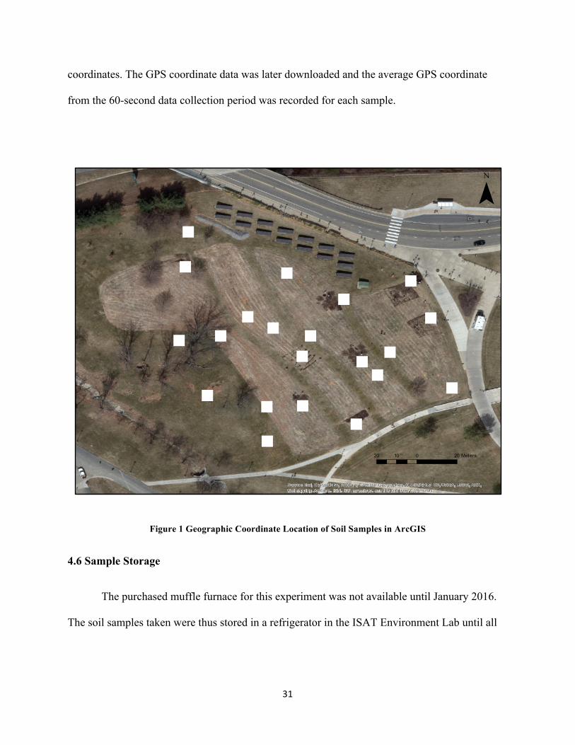
coordinates. The GPS coordinate data was later downloaded and the average GPS coordinate

from the 60-second data collection period was recorded for each sample.

Figure 1 Geographic Coordinate Location of Soil Samples in ArcGIS

4.6 Sample Storage

The purchased muffle furnace for this experiment was not available until January 2016.

The soil samples taken were thus stored in a refrigerator in the ISAT Environment Lab until all

"

"

"

"

"

""

"

"

"

"

"

""

"

"

""

"

""

"

Source: Esri, DigitalGlobe, GeoEye, Earthstar Geographics, CNES/Airbus DS, USDA, USGS, AEX,Getmapping, Aerogrid, IGN, IGP, swisstopo, and the GIS User Community

¯

20 0 2010 Meters

32

the necessary equipment was available. All samples were placed in individual plastic bags with

their accompanying soil sample ID, sample date, and time of sample.

4.7 Sample Conditioning

Before the samples could be dried using the muffle furnace, they were mixed because

they had remained stagnant in the refrigerator for two months. In the first two replications of this

experiment, the soil samples were manually mixed by hand. The plastic bags containing the soil

samples were shaken and mixed by hand. To improve the mixing procedure and determine if

different mixing protocols yielded differing results, the soil samples were mechanically mixed in

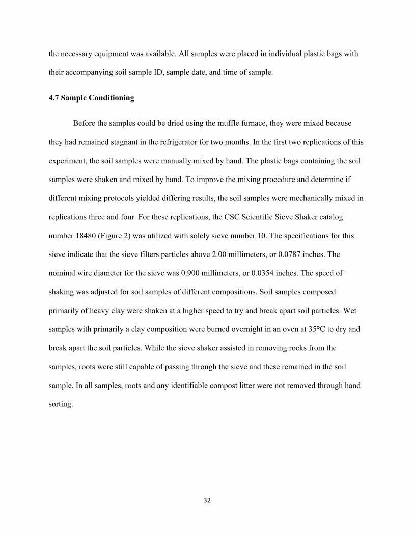
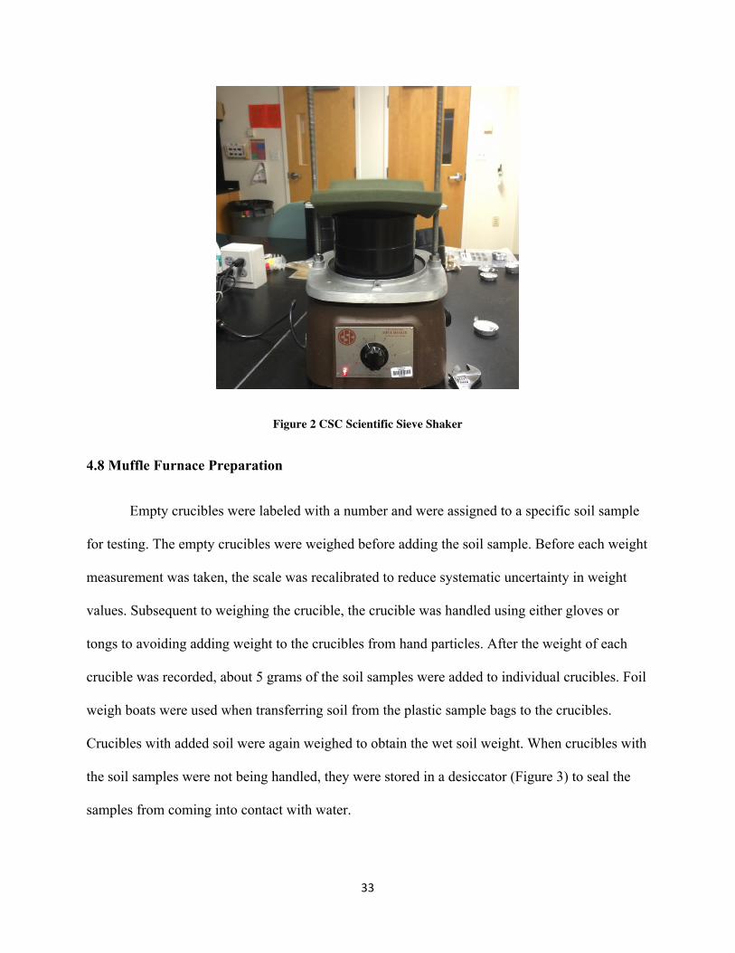
replications three and four. For these replications, the CSC Scientific Sieve Shaker catalog

number 18480 (Figure 2) was utilized with solely sieve number 10. The specifications for this

sieve indicate that the sieve filters particles above 2.00 millimeters, or 0.0787 inches. The

nominal wire diameter for the sieve was 0.900 millimeters, or 0.0354 inches. The speed of

shaking was adjusted for soil samples of different compositions. Soil samples composed

primarily of heavy clay were shaken at a higher speed to try and break apart soil particles. Wet

samples with primarily a clay composition were burned overnight in an oven at 35°C to dry and

break apart the soil particles. While the sieve shaker assisted in removing rocks from the

samples, roots were still capable of passing through the sieve and these remained in the soil

sample. In all samples, roots and any identifiable compost litter were not removed through hand

sorting.

33

Figure 2 CSC Scientific Sieve Shaker

4.8 Muffle Furnace Preparation

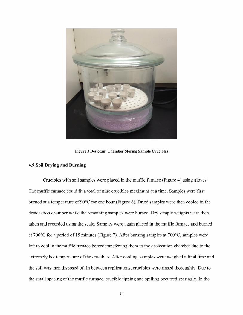
Empty crucibles were labeled with a number and were assigned to a specific soil sample

for testing. The empty crucibles were weighed before adding the soil sample. Before each weight

measurement was taken, the scale was recalibrated to reduce systematic uncertainty in weight

values. Subsequent to weighing the crucible, the crucible was handled using either gloves or

tongs to avoiding adding weight to the crucibles from hand particles. After the weight of each

crucible was recorded, about 5 grams of the soil samples were added to individual crucibles. Foil

weigh boats were used when transferring soil from the plastic sample bags to the crucibles.

Crucibles with added soil were again weighed to obtain the wet soil weight. When crucibles with

the soil samples were not being handled, they were stored in a desiccator (Figure 3) to seal the

samples from coming into contact with water.

34

Figure 3 Desiccant Chamber Storing Sample Crucibles

4.9 Soil Drying and Burning

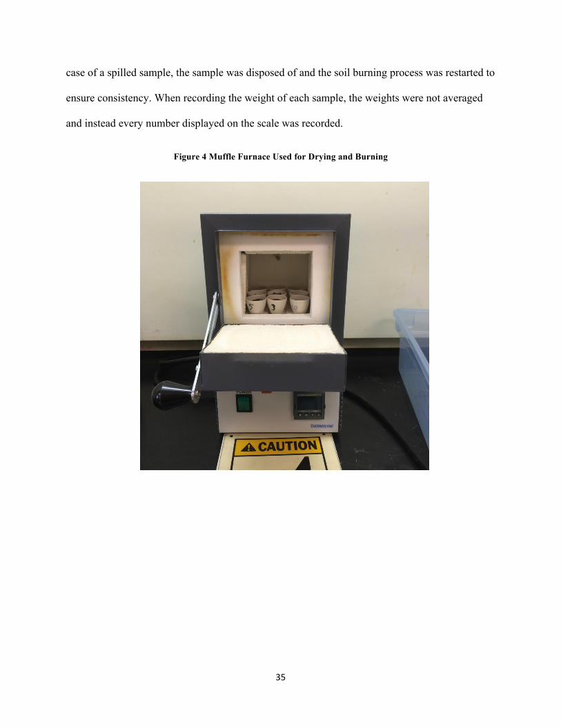
Crucibles with soil samples were placed in the muffle furnace (Figure 4) using gloves.

The muffle furnace could fit a total of nine crucibles maximum at a time. Samples were first

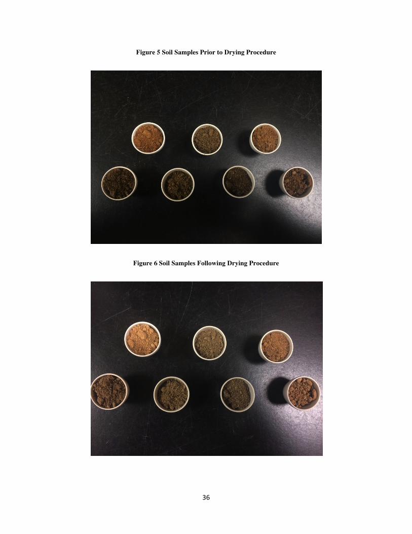
burned at a temperature of 90°C for one hour (Figure 6). Dried samples were then cooled in the

desiccation chamber while the remaining samples were burned. Dry sample weights were then

taken and recorded using the scale. Samples were again placed in the muffle furnace and burned

at 700°C for a period of 15 minutes (Figure 7). After burning samples at 700°C, samples were

left to cool in the muffle furnace before transferring them to the desiccation chamber due to the

extremely hot temperature of the crucibles. After cooling, samples were weighed a final time and

the soil was then disposed of. In between replications, crucibles were rinsed thoroughly. Due to

the small spacing of the muffle furnace, crucible tipping and spilling occurred sparingly. In the

35

case of a spilled sample, the sample was disposed of and the soil burning process was restarted to

ensure consistency. When recording the weight of each sample, the weights were not averaged

and instead every number displayed on the scale was recorded.

Figure 4 Muffle Furnace Used for Drying and Burning

36

Figure 5 Soil Samples Prior to Drying Procedure

Figure 6 Soil Samples Following Drying Procedure

37

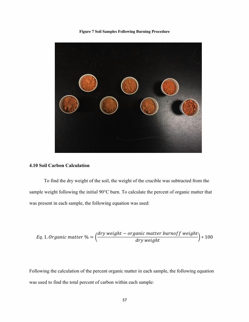
Figure 7 Soil Samples Following Burning Procedure

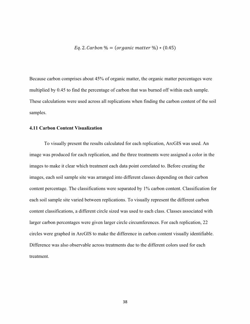
4.10 Soil Carbon Calculation

To find the dry weight of the soil, the weight of the crucible was subtracted from the

sample weight following the initial 90°C burn. To calculate the percent of organic matter that

was present in each sample, the following equation was used:

𝐸𝑞. 1.𝑂𝑟𝑔𝑎𝑛𝑖𝑐 𝑚𝑎𝑡𝑡𝑒𝑟 % =𝑑𝑟𝑦 𝑤𝑒𝑖𝑔ℎ𝑡 − 𝑜𝑟𝑔𝑎𝑛𝑖𝑐 𝑚𝑎𝑡𝑡𝑒𝑟 𝑏𝑢𝑟𝑛𝑜𝑓𝑓 𝑤𝑒𝑖𝑔ℎ𝑡

𝑑𝑟𝑦 𝑤𝑒𝑖𝑔ℎ𝑡 ∗ 100

Following the calculation of the percent organic matter in each sample, the following equation

was used to find the total percent of carbon within each sample:

38

𝐸𝑞. 2.𝐶𝑎𝑟𝑏𝑜𝑛 % = 𝑜𝑟𝑔𝑎𝑛𝑖𝑐 𝑚𝑎𝑡𝑡𝑒𝑟 % ∗ (0.45)

Because carbon comprises about 45% of organic matter, the organic matter percentages were

multiplied by 0.45 to find the percentage of carbon that was burned off within each sample.

These calculations were used across all replications when finding the carbon content of the soil

samples.

4.11 Carbon Content Visualization

To visually present the results calculated for each replication, ArcGIS was used. An

image was produced for each replication, and the three treatments were assigned a color in the

images to make it clear which treatment each data point correlated to. Before creating the

images, each soil sample site was arranged into different classes depending on their carbon

content percentage. The classifications were separated by 1% carbon content. Classification for

each soil sample site varied between replications. To visually represent the different carbon

content classifications, a different circle sized was used to each class. Classes associated with

larger carbon percentages were given larger circle circumferences. For each replication, 22

circles were graphed in ArcGIS to make the difference in carbon content visually identifiable.

Difference was also observable across treatments due to the different colors used for each

treatment.

39

4.12 Statistical Analysis

To execute a statistical analysis of the data collected, GraphPad Scientific Software was

utilized. The software was used to perform an unpaired two-tailed t-test to compare two means.

This was executed three times for each replication so that each treatment could be compared to

each other. The average carbon content was compared for compost amendment vs. no compost

amendment, compost amendment vs. lawn, and no compost amendment vs. lawn. Each run on

the statistical software produced the two-tailed p value, the 95% confidence interval of the

difference, the t value used, the degrees of freedom, and the standard error of difference in the

data. This permitted determination of whether or not the difference between treatments was

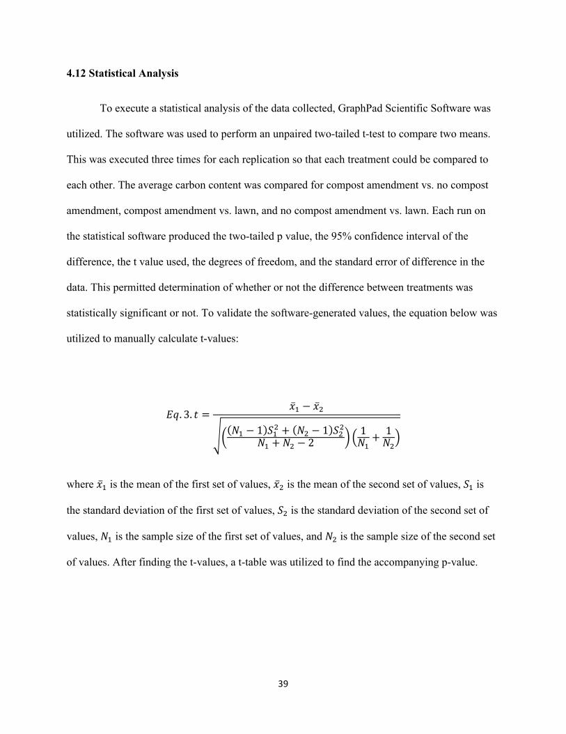
statistically significant or not. To validate the software-generated values, the equation below was

utilized to manually calculate t-values:

𝐸𝑞. 3. 𝑡 =𝑥! − 𝑥!

𝑁! − 1 𝑆!! + 𝑁! − 1 𝑆!!𝑁! + 𝑁! − 2

1𝑁!+ 1𝑁!

where 𝑥! is the mean of the first set of values, 𝑥! is the mean of the second set of values, 𝑆! is

the standard deviation of the first set of values, 𝑆! is the standard deviation of the second set of

values, 𝑁! is the sample size of the first set of values, and 𝑁! is the sample size of the second set

of values. After finding the t-values, a t-table was utilized to find the accompanying p-value.

40

Chapter 5 Results

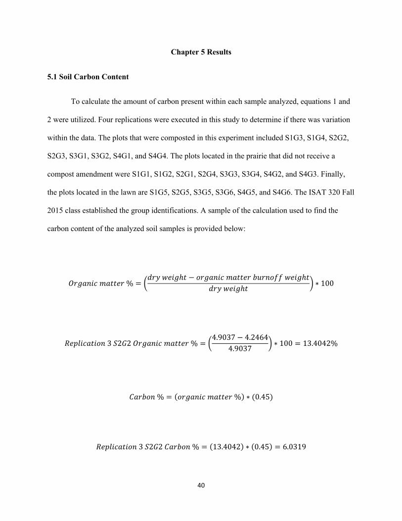
5.1 Soil Carbon Content

To calculate the amount of carbon present within each sample analyzed, equations 1 and

2 were utilized. Four replications were executed in this study to determine if there was variation

within the data. The plots that were composted in this experiment included S1G3, S1G4, S2G2,

S2G3, S3G1, S3G2, S4G1, and S4G4. The plots located in the prairie that did not receive a

compost amendment were S1G1, S1G2, S2G1, S2G4, S3G3, S3G4, S4G2, and S4G3. Finally,

the plots located in the lawn are S1G5, S2G5, S3G5, S3G6, S4G5, and S4G6. The ISAT 320 Fall

2015 class established the group identifications. A sample of the calculation used to find the

carbon content of the analyzed soil samples is provided below:

𝑂𝑟𝑔𝑎𝑛𝑖𝑐 𝑚𝑎𝑡𝑡𝑒𝑟 % =𝑑𝑟𝑦 𝑤𝑒𝑖𝑔ℎ𝑡 − 𝑜𝑟𝑔𝑎𝑛𝑖𝑐 𝑚𝑎𝑡𝑡𝑒𝑟 𝑏𝑢𝑟𝑛𝑜𝑓𝑓 𝑤𝑒𝑖𝑔ℎ𝑡

𝑑𝑟𝑦 𝑤𝑒𝑖𝑔ℎ𝑡 ∗ 100

𝑅𝑒𝑝𝑙𝑖𝑐𝑎𝑡𝑖𝑜𝑛 3 𝑆2𝐺2 𝑂𝑟𝑔𝑎𝑛𝑖𝑐 𝑚𝑎𝑡𝑡𝑒𝑟 % =4.9037− 4.2464

4.9037 ∗ 100 = 13.4042%

𝐶𝑎𝑟𝑏𝑜𝑛 % = 𝑜𝑟𝑔𝑎𝑛𝑖𝑐 𝑚𝑎𝑡𝑡𝑒𝑟 % ∗ (0.45)

𝑅𝑒𝑝𝑙𝑖𝑐𝑎𝑡𝑖𝑜𝑛 3 𝑆2𝐺2 𝐶𝑎𝑟𝑏𝑜𝑛 % = 13.4042 ∗ 0.45 = 6.0319

41

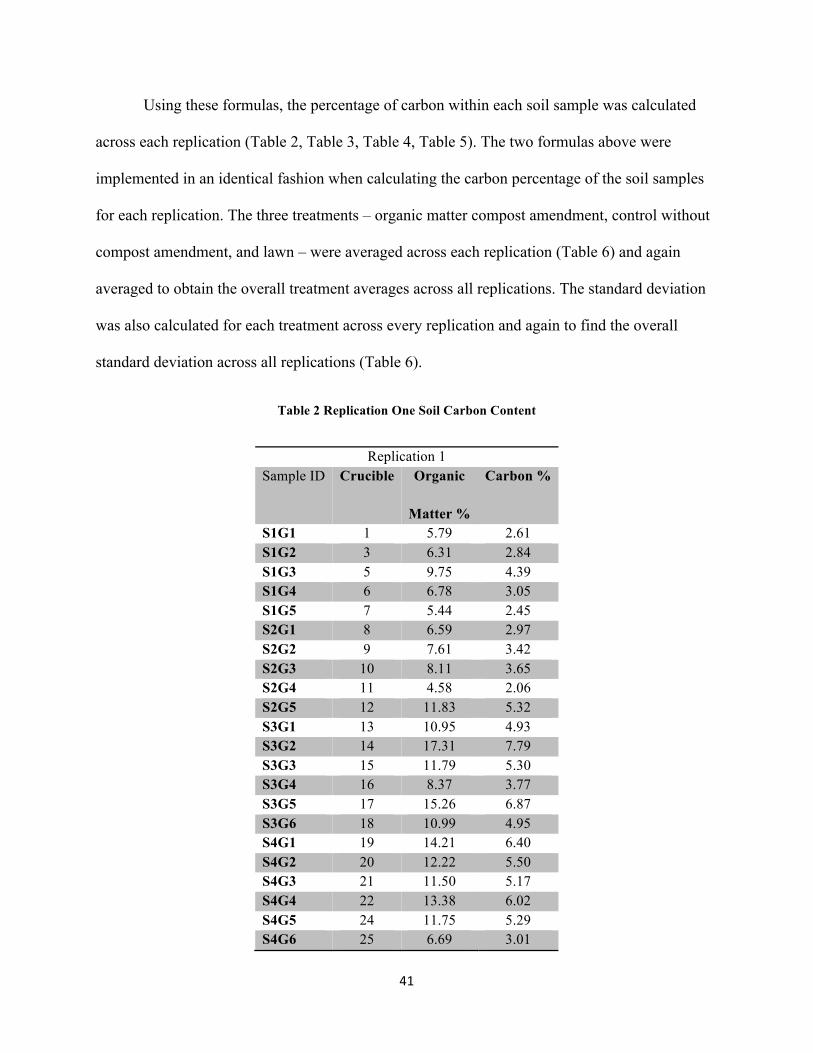
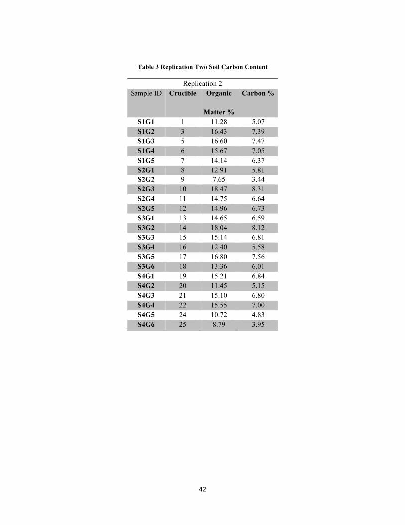
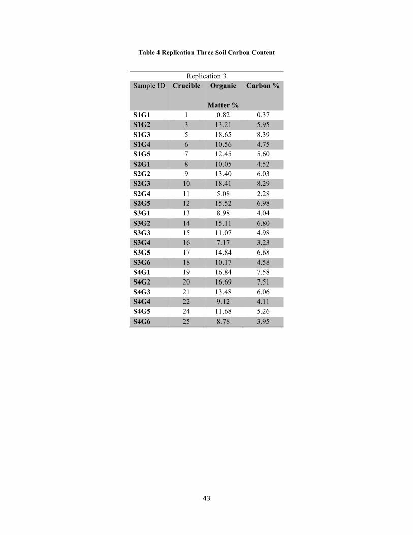
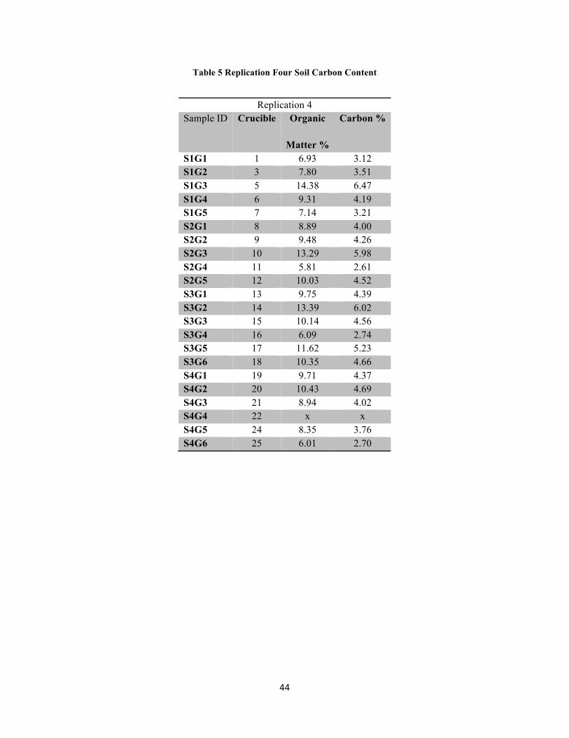
Using these formulas, the percentage of carbon within each soil sample was calculated

across each replication (Table 2, Table 3, Table 4, Table 5). The two formulas above were

implemented in an identical fashion when calculating the carbon percentage of the soil samples

for each replication. The three treatments – organic matter compost amendment, control without

compost amendment, and lawn – were averaged across each replication (Table 6) and again

averaged to obtain the overall treatment averages across all replications. The standard deviation

was also calculated for each treatment across every replication and again to find the overall

standard deviation across all replications (Table 6).

Table 2 Replication One Soil Carbon Content

Replication 1 Sample ID Crucible Organic

Matter %

Carbon %

S1G1 1 5.79 2.61 S1G2 3 6.31 2.84 S1G3 5 9.75 4.39 S1G4 6 6.78 3.05 S1G5 7 5.44 2.45 S2G1 8 6.59 2.97 S2G2 9 7.61 3.42 S2G3 10 8.11 3.65 S2G4 11 4.58 2.06 S2G5 12 11.83 5.32 S3G1 13 10.95 4.93 S3G2 14 17.31 7.79 S3G3 15 11.79 5.30 S3G4 16 8.37 3.77 S3G5 17 15.26 6.87 S3G6 18 10.99 4.95 S4G1 19 14.21 6.40 S4G2 20 12.22 5.50 S4G3 21 11.50 5.17 S4G4 22 13.38 6.02 S4G5 24 11.75 5.29 S4G6 25 6.69 3.01

42

Table 3 Replication Two Soil Carbon Content


Matter %

Carbon %


43

Table 4 Replication Three Soil Carbon Content


Matter %

Carbon %


44

Table 5 Replication Four Soil Carbon Content


Matter %

Carbon %

S1G1 1 6.93 3.12 S1G2 3 7.80 3.51 S1G3 5 14.38 6.47 S1G4 6 9.31 4.19 S1G5 7 7.14 3.21 S2G1 8 8.89 4.00 S2G2 9 9.48 4.26 S2G3 10 13.29 5.98 S2G4 11 5.81 2.61 S2G5 12 10.03 4.52 S3G1 13 9.75 4.39 S3G2 14 13.39 6.02 S3G3 15 10.14 4.56 S3G4 16 6.09 2.74 S3G5 17 11.62 5.23 S3G6 18 10.35 4.66 S4G1 19 9.71 4.37 S4G2 20 10.43 4.69 S4G3 21 8.94 4.02 S4G4 22 x x S4G5 24 8.35 3.76 S4G6 25 6.01 2.70

45

Table 6 Average Soil Carbon Content Across All Replications

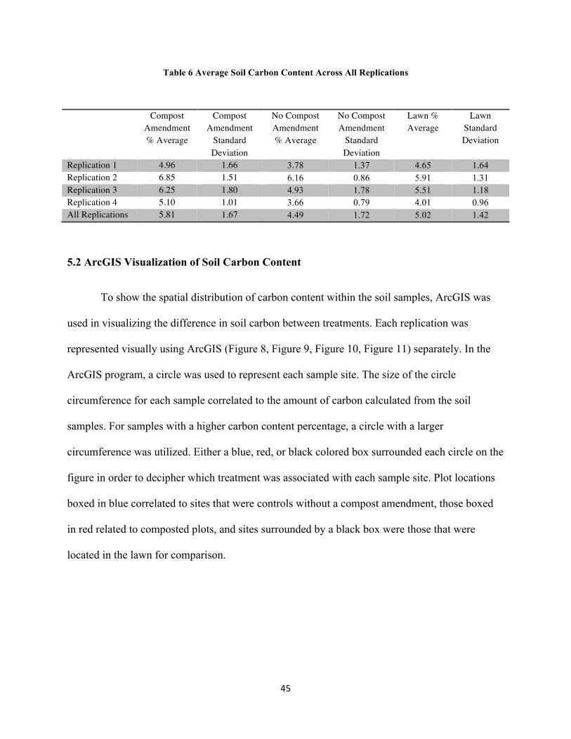
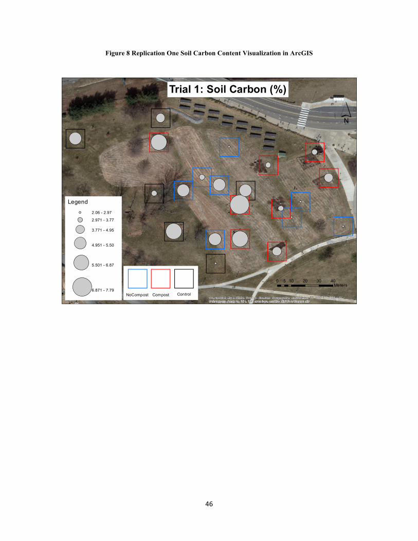
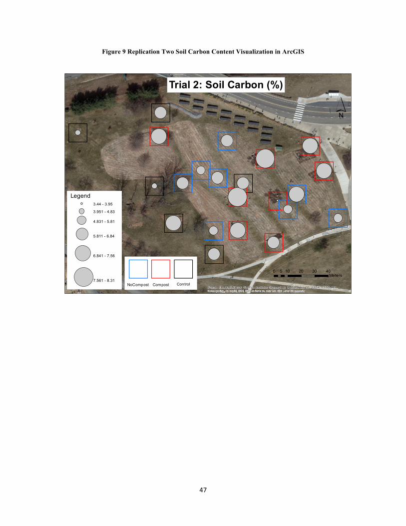
5.2 ArcGIS Visualization of Soil Carbon Content

To show the spatial distribution of carbon content within the soil samples, ArcGIS was

used in visualizing the difference in soil carbon between treatments. Each replication was

represented visually using ArcGIS (Figure 8, Figure 9, Figure 10, Figure 11) separately. In the

ArcGIS program, a circle was used to represent each sample site. The size of the circle

circumference for each sample correlated to the amount of carbon calculated from the soil

samples. For samples with a higher carbon content percentage, a circle with a larger

circumference was utilized. Either a blue, red, or black colored box surrounded each circle on the

figure in order to decipher which treatment was associated with each sample site. Plot locations

boxed in blue correlated to sites that were controls without a compost amendment, those boxed

in red related to composted plots, and sites surrounded by a black box were those that were

located in the lawn for comparison.

Compost Amendment % Average

Compost Amendment

Standard Deviation

No Compost Amendment % Average

No Compost Amendment

Standard Deviation

Lawn % Average

Lawn Standard Deviation

Replication 1 4.96 1.66 3.78 1.37 4.65 1.64 Replication 2 6.85 1.51 6.16 0.86 5.91 1.31 Replication 3 6.25 1.80 4.93 1.78 5.51 1.18 Replication 4 5.10 1.01 3.66 0.79 4.01 0.96 All Replications 5.81 1.67 4.49 1.72 5.02 1.42

46

Figure 8 Replication One Soil Carbon Content Visualization in ArcGIS

))

))

)

))

))

)

)

)))

)

)

))

)

))

)


´Trial 1: Soil Carbon (%)

Legend

2.06 - 2.97

2.971 - 3.77

3.771 - 4.95

4.951 - 5.50

5.501 - 6.87

6.871 - 7.79

0 10 20 30 405Meters)

NoCompost

)Compost

)Control

47

Figure 9 Replication Two Soil Carbon Content Visualization in ArcGIS

))

))

)

))

))

)

)

)))

)

)

))

)

))

)



0 10 20 30 405Meters)

NoCompost

)Compost

)Control

Legend3.44 - 3.95

3.951 - 4.83

4.831 - 5.81

5.811 - 6.84

6.841 - 7.56

7.561 - 8.31

48

Figure 10 Replication Three Soil Carbon Content Visualization in ArcGIS

))

))

)

))

))

)

)

)))

)

)

))

)

))

)



0 10 20 30 405Meters)

NoCompost

)Compost

)Control

Legend3.44 - 3.95

3.951 - 4.83

4.831 - 5.81

5.811 - 6.84

6.841 - 7.56

7.561 - 8.31

Legend

0.36 - 2.28

2.281 - 3.95

3.951 - 4.95

4.951 - 5.95

5.951 - 6.98

6.981 - 7.58

7.581 - 8.39

49

Figure 11 Replication Four Soil Carbon Content Visualization in ArcGIS

5.3 Statistical Analysis Between Treatments

To determine if the differences between treatments in this experiment were considered to

be statistically significant, an unpaired two-tailed t-test was executed to compare the three

treatments for each replication. GraphPad Scientific Software was utilized to calculate the p-

values, and the values were manually verified. To validate the software-generated values,

equation three was utilized in manually calculating the t-values.

))

))

)

))

))

)

)

)))

)

)

))

)

))

)



0 10 20 30 405Meters)

NoCompost

)Compost

)Control

Legend2.61 - 2.74

2.741 - 3.76

3.761 - 4.69

4.691 - 5.98

5.981 - 6.47

50

by calculating t-values and using a t-table to find the accompanying p-value. An example of the

t-value calculation is provided below.

𝐸𝑞. 3. 𝑡 =𝑥! − 𝑥!

𝑁! − 1 𝑆!! + 𝑁! − 1 𝑆!!𝑁! + 𝑁! − 2

1𝑁!+ 1𝑁!

𝑡 =4.9556− 3.7773

8− 1 1.6578! + 8− 1 1.3685!8+ 8− 2

18+

18

= 1.5505

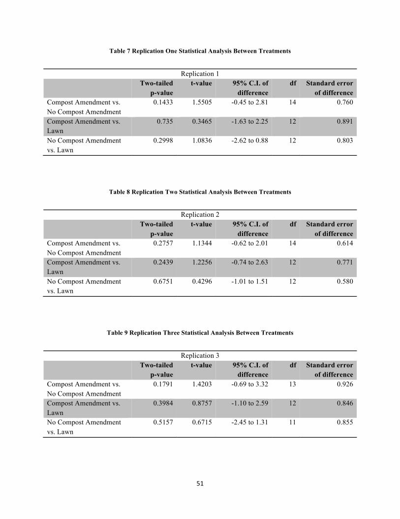
The two-tailed p-values were calculated to compare compost amendment vs. no compost

amendment, compost amendment vs. lawn, and no compost amendment vs. lawn. This procedure

was completed for each replication (Table 7, Table 8, Table 9, Table 10) rather than combining

each replication into a single statistical analysis. The replications were kept separate during

statistical analysis due to variation observed between replications. The statistical analysis

software also reported the 95% confidence interval of difference and the standard error of

difference, both of which were recorded.

51

Table 7 Replication One Statistical Analysis Between Treatments

Replication 1 Two-tailed

p-value t-value 95% C.I. of

difference df Standard error

of difference Compost Amendment vs. No Compost Amendment

0.1433 1.5505 -0.45 to 2.81 14 0.760

Compost Amendment vs. Lawn

0.735 0.3465 -1.63 to 2.25 12 0.891

No Compost Amendment vs. Lawn

0.2998 1.0836 -2.62 to 0.88 12 0.803

Table 8 Replication Two Statistical Analysis Between Treatments





0.2757 1.1344 -0.62 to 2.01 14 0.614


0.2439 1.2256 -0.74 to 2.63 12 0.771


0.6751 0.4296 -1.01 to 1.51 12 0.580

Table 9 Replication Three Statistical Analysis Between Treatments





0.1791 1.4203 -0.69 to 3.32 13 0.926


0.3984 0.8757 -1.10 to 2.59 12 0.846


0.5157 0.6715 -2.45 to 1.31 11 0.855

52

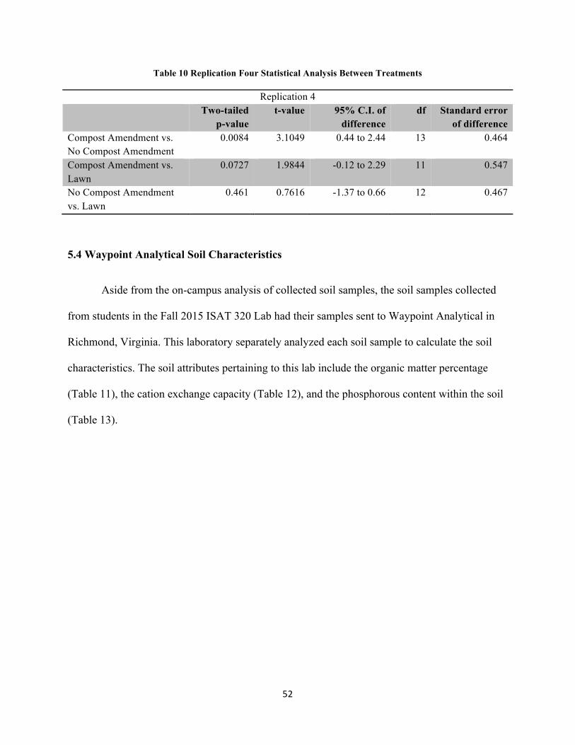
Table 10 Replication Four Statistical Analysis Between Treatments





0.0084 3.1049 0.44 to 2.44 13 0.464


0.0727 1.9844 -0.12 to 2.29 11 0.547


0.461 0.7616 -1.37 to 0.66 12 0.467

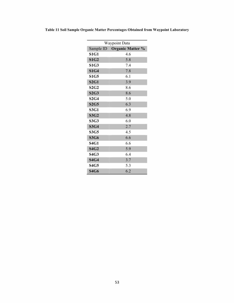
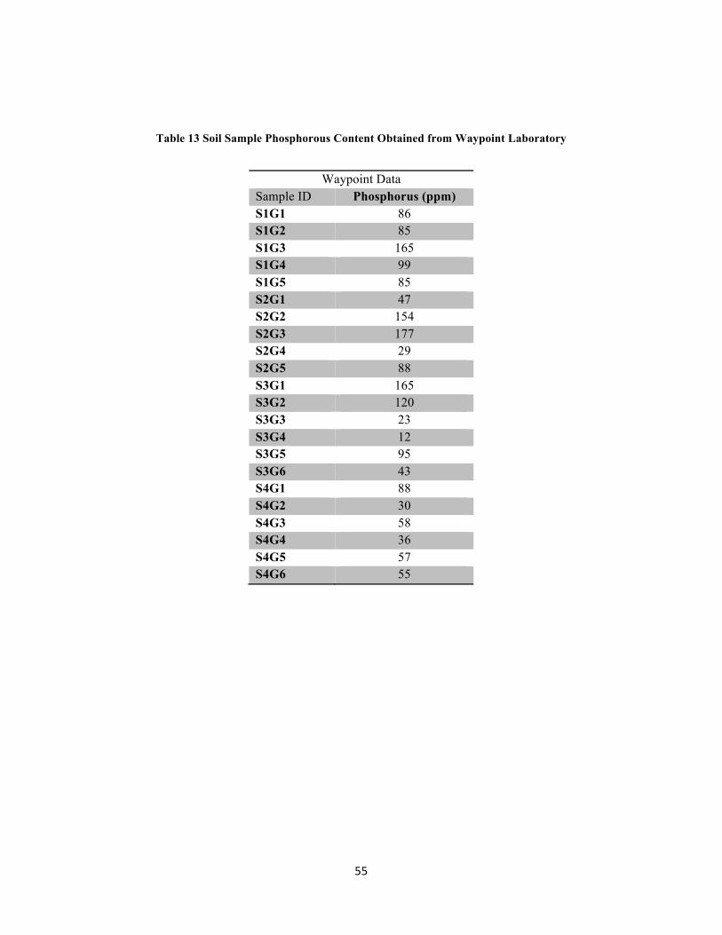
5.4 Waypoint Analytical Soil Characteristics

Aside from the on-campus analysis of collected soil samples, the soil samples collected

from students in the Fall 2015 ISAT 320 Lab had their samples sent to Waypoint Analytical in

Richmond, Virginia. This laboratory separately analyzed each soil sample to calculate the soil

characteristics. The soil attributes pertaining to this lab include the organic matter percentage

(Table 11), the cation exchange capacity (Table 12), and the phosphorous content within the soil

(Table 13).

53

Table 11 Soil Sample Organic Matter Percentages Obtained from Waypoint Laboratory

Waypoint Data Sample ID Organic Matter % S1G1 4.6 S1G2 5.8 S1G3 7.4 S1G4 7.8 S1G5 6.1 S2G1 3.9 S2G2 8.6 S2G3 8.6 S2G4 5.0 S2G5 6.3 S3G1 6.9 S3G2 4.8 S3G3 6.0 S3G4 2.7 S3G5 4.5 S3G6 6.6 S4G1 6.6 S4G2 5.9 S4G3 6.4 S4G4 3.7 S4G5 5.3 S4G6 6.2

54

Table 12 Soil Sample Cation Exchange Capacity Obtained from Waypoint Laboratory

Waypoint Data Sample ID Cation Exchange

Capacity (meg/100g) S1G1 7.3 S1G2 10.2 S1G3 11.8 S1G4 13.8 S1G5 24.2 S2G1 6.8 S2G2 15.3 S2G3 18.7 S2G4 7.2 S2G5 12.0 S3G1 13.3 S3G2 11.4 S3G3 12.7 S3G4 8.6 S3G5 8.8 S3G6 10.1 S4G1 12.2 S4G2 27.1 S4G3 25.8 S4G4 11.3 S4G5 13.2 S4G6 18.7

55

Table 13 Soil Sample Phosphorous Content Obtained from Waypoint Laboratory

Waypoint Data Sample ID Phosphorus (ppm) S1G1 86 S1G2 85 S1G3 165 S1G4 99 S1G5 85 S2G1 47 S2G2 154 S2G3 177 S2G4 29 S2G5 88 S3G1 165 S3G2 120 S3G3 23 S3G4 12 S3G5 95 S3G6 43 S4G1 88 S4G2 30 S4G3 58 S4G4 36 S4G5 57 S4G6 55

56

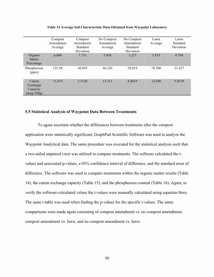
Table 14 Average Soil Characteristic Data Obtained from Waypoint Laboratory

Compost Amendment

Average

Compost Amendment

Standard Deviation


Average


Standard Deviation

Lawn Average

Lawn Standard Deviation

Organic Matter

Percentage

6.800

1.753

5.038

1.257

5.833

0.784

Phosphorous

(ppm) 125.50

48.893

46.250

28.019

70.500

21.427

Cation

Exchange Capacity

(meg/100g)

13.475

2.5138

13.213

8.4019

14.500

5.8570

5.5 Statistical Analysis of Waypoint Data Between Treatments

To again ascertain whether the differences between treatments after the compost

application were statistically significant, GraphPad Scientific Software was used to analyze the

Waypoint Analytical data. The same procedure was executed for the statistical analysis such that

a two-tailed unpaired t-test was utilized to compare treatments. The software calculated the t-

values and associated p-values, a 95% confidence interval of difference, and the standard error of

difference. The software was used to compare treatments within the organic matter results (Table

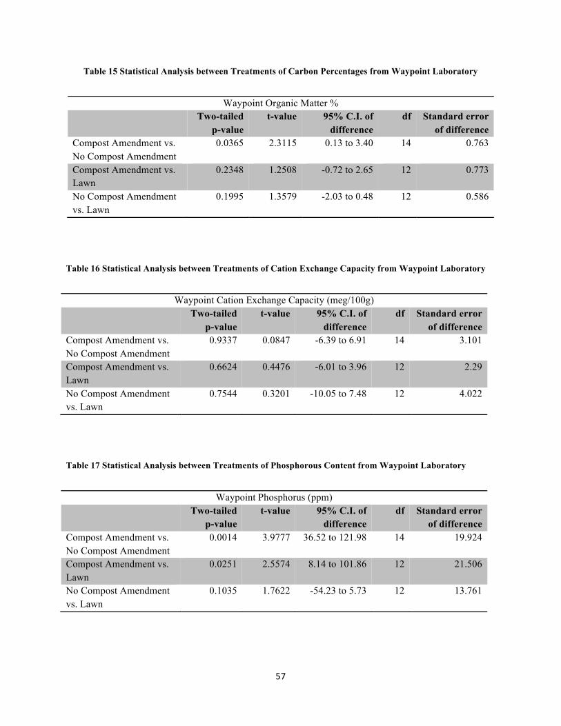
14), the cation exchange capacity (Table 15), and the phosphorous content (Table 16). Again, to

verify the software-calculated values the t-values were manually calculated using equation three.

The same t-table was used when finding the p-values for the specific t-values. The same

comparisons were made again consisting of compost amendment vs. no compost amendment,

compost amendment vs. lawn, and no compost amendment vs. lawn.

57

Table 15 Statistical Analysis between Treatments of Carbon Percentages from Waypoint Laboratory

Waypoint Organic Matter % Two-tailed




0.0365 2.3115 0.13 to 3.40 14 0.763


0.2348 1.2508 -0.72 to 2.65 12 0.773


0.1995 1.3579 -2.03 to 0.48 12 0.586

Table 16 Statistical Analysis between Treatments of Cation Exchange Capacity from Waypoint Laboratory

Waypoint Cation Exchange Capacity (meg/100g) Two-tailed




0.9337 0.0847 -6.39 to 6.91 14 3.101


0.6624 0.4476 -6.01 to 3.96 12 2.29


0.7544 0.3201 -10.05 to 7.48 12 4.022

Table 17 Statistical Analysis between Treatments of Phosphorous Content from Waypoint Laboratory

Waypoint Phosphorus (ppm) Two-tailed




0.0014 3.9777 36.52 to 121.98 14 19.924


0.0251 2.5574 8.14 to 101.86 12 21.506


0.1035 1.7622 -54.23 to 5.73 12 13.761

58

Chapter 6 Discussion

6.1 Soil Carbon Content Interpretation

After executing four replications of analyzing carbon content from the soil samples, it was

found that on average, the plots that received a compost amendment had the highest soil carbon

content. There was variation observed between replications (Table 2, Table 3, Table 4, Table 5),

which was likely due to a number of factors that introduced uncertainty into the measurements.

The average carbon content of the composted plots varied from 4.96 percent to 6.85 percent

(Table 6). In the prairie plots that didn’t receive a compost amendment, the percentage of carbon

found within the soil ranged from 3.66 percent to 6.16 percent (Table 6). For the lawn plots, the

soil carbon content varies from 4.01 percent to 5.91 percent (Table 6). Although there was

variation across replications, the trend observed was that the composted plots had, on average,

the highest percentage of soil carbon with a total average of 5.81 +/- 1.67 percent (Table 6). The

lawn plots had the second highest carbon content with an average percentage of 5.02 +/- 1.42

(Table 6). The lawn plots had a higher carbon content that the non-composted prairie plots due to

high root abundance found within the lawn soil samples. Finally, the prairie plots without the

compost amendment had the lowest carbon percentage average of 4.49 +/- 1.72 (Table 6). This

aligns with the initially stated hypothesis that plots receiving a single compost amendment would

have the highest percent of carbon within the soil.

The calculated percentage of carbon within each soil sample follows the trend observed in

the Marin Carbon Project in which plots have a higher amount of carbon sequestration after

receiving an organic matter amendment. Aside from the presentation of quantitative results, these

values were analyzed spatially in ArcGIS (Figure 8, Figure 9, Figure 10, Figure 11). Looking at

59

the images produced from the software, the trends are again observable. In replication one

(Figure 8), the composted plots on average are associated with the largest circle size – meaning

their carbon content is higher. The plots boxed in blue, which were located on the prairie but

were not composted, have a much smaller percentage of soil carbon than the composted and

lawn plots. There is variation within the data such that plots within each treatment exhibited

diversity in results for soil carbon content. In replication two (Figure 9), the composted plots

again exhibit the highest percentage of soil carbon. The values obtained in replication two vary

from replication one because the calculated values for each treatment were on average higher in

replication two than they were in replication one. In replication three (Figure 10), the results are

similar to those found in replication two (Figure 9). The same overall trend is observable that the

plots with the compost amendment have the highest percentage of soil carbon sequestered. The

plots located in the lawn again have a higher soil carbon content than the non-composted prairie

plots, which is accounted for by the high abundance of roots within the lawn. In replication four

(Figure 11), the results are similar to those found in replication one (Figure 8). While there is

again variation amongst treatments, the same trend is observable in the average soil carbon

content between treatments.

While the averages of the soil carbon percentages indicate that the compost amendment

successfully boosted the carbon sequestration in comparison to the control and lawn plots,

uncertainty within this study created variation in results between replications and amongst

treatments. Although the same trends were observable when analyzing the overall averages of

each replication, there is variation in the data. The composted plots have the highest percentage

of soil carbon, but the value calculated for a particular sample often varied between replications.

For example, the percentage of carbon measured in sample S1G3 was 4.39 percent in replication

60

one (Table 2), but when this same sample was analyzed again in replication two, the percentage

found was 7.47 (Table 3). The percentage found varied again in replications three in four, as a

value of 8.39 percent was calculated in replication three (Table 4), and a percentage of 6.47 was

found in replication four (Table 5). Because the data varied between replications, it was difficult

comparing the ArcGIS images to each other because each replication yielded different results.

Aside from variation between replications, there was also disparity within the same treatments.

In replication one (Table 2), for example, the percentage of soil carbon found in sample S3G2

was 7.79, while the percentage for S1G4 was 3.05. Although both of these plots received an

identical organic matter amendment, there is a significant difference between the soil carbon

content found. This can either be attributed to natural spatial variation or uncertainty within

measurements.

There are multiple notions pertaining to why there was such high variation in results within

this study. The first is that the procedure for mixing the soil prior to placing it within the crucible

was altered after executing the first two replications. In replications one and two, the sample was

manually mixed by shaking the plastic bag with the soil sample. Because there was variation

observed between replications one and two, it was predicted that the mixing method was not

efficiently mixing the soil samples – which may have caused disparity in the results. The mixing

procedure was consequently altered to acquire soil samples with thorough mixing. For

replications three and four, the samples were mixed using a scientific sieve shaker. Only the

sieve #10 was used in this procedure, which filters particles at 2.00 millimeters, or 0.0787 inches.

Although this sample mixing procedure was enhanced, there was still variation within the results

obtained from replication three (Table 4) and replication four (Table 5). Because the soil shaking

technique was not an identical procedure utilized for all four replications, difference between the

61

results across replications is in part due to this.

Another area of introduced uncertainty within this study is the high root abundance found

within soil samples. This factor is likely the main contributor to the variation found across

replications and within treatments. A high amount of roots within the soil samples offsets the

weight output of the scales, thus influencing the total organic matter and carbon percentage

calculated from the weight measurements. Even when executing the sieve shaker soil mixing

procedure, the roots still passed through the sieve. These root particles were not manually

removed from the soil samples and were thus included in the dried and burned weights. There

was spatial difference in the carbon content, which is likely due to the diverse plant species

altering the results differently. Because plant diversity and density was not incorporated into this

study, it was not possible to determine how these plant roots were specifically altering the

measured carbon content of each soil sample. Although the degree to which plant roots affected

the results cannot be quantified, the source of uncertainty was identified and be incorporated into

future studies so that the extent of plant root influence can be quantified and thoroughly

analyzed.

Another route for uncertainty within these measurements is the rocky and shallow

conditions of the soil where the samples were collected. Due to these conditions, it was difficult

to penetrate the soil and collect a sample at an ideal depth. To maintain uniformity within soil

sample collection, every sample was collected from a depth of six inches. At some sample

locations, obtaining a sample depth of even six inches was extremely difficult due to a high

abundance of rocks within the soil. An ideal sample depth in this particular type of study is 20

centimeters, or roughly eight inches. This depth was not obtainable in this experiment due to its

rocky conditions. With an enhanced procedure or sampling equipment, soil samples could be

62

collected at a depth of eight inches to thus boost the accuracy of the carbon content results. In

replications one and two, the sieve shaker was not implemented into the procedure and there was

a higher abundance of rocks included in the sample as it was dried and burned. The presence of

rocks offsets the weights and ultimately altered the soil carbon content calculation. Because

some plots had a greater wealth of rocks, the calculated soil carbon content was more greatly

affected due to the added weight of rocks. Overcoming this requires sieve shaking in all

replications and confirming that the sieve size was appropriate for removing most to all of the

rock fragments. The abundance of rocks was not entirely overcome in this experiment, indicating

that the rocky and shallow properties of the study site contributed to the uncertainty and variation

within results.

The study site in this experiment previously had a dirt road that ran directly through it.

When James Madison University purchased the land, maintenance facilities planted directly over

the dirt road. Although the road was covered in vegetation, the previous usage of the road

compacted the soil underneath it. As a result, vegetation has more difficulty extending its roots

into the soil. Overcoming soil compaction takes a significant amount of time for the roots to

loosen the soil and make it more fertile. Plots located in the close proximity to where the road

previously ran likely have more difficulty flourishing due to stunted root growth in the

compacted soil. While this was not integrated into this study, it is probable that the soil

compaction from the dirt road affected the ability for some plots to boost their organic matter

percentage. Plants need to extend their roots deep into the soil to come into contact with the

beneficial soil microbes that assist in building topsoil. If plant growth is stunted due to

compacted soil, it becomes more difficult for plant development to be heightened following a

composted organic matter amendment. If this occurs, plants are less likely to have extensive

63

relationships with soil microbes, meaning less of the root exudates from soil will be transformed

into stable humus. The extensive impacts of compacted soil consequently contributed to spatial

differences in soil carbon content found amongst soil samples.

Uncertainty in the measurements can also stem from measuring devices and human error.

Although the scale was recalibrated prior to each collected measurement, it is possible for the

scale to report inaccurate results. When obtaining the weights for each soil sample, the number

read off the scale was rarely steady. The number often wobbled back and forth between a

significant figure, and slowly changed value as the sample was held on the scale. This indicates

that were was inherently uncertainty within the weight values obtained from the scale. While this

is unlikely to greatly affect the data obtained, it still remains a source of uncertainty within this

study. Manually working within the laboratory also generates opportunities for human error to

occur. Caution was always taken to strictly follow the same procedure, but it is impossible to

completely avoid human error within experiments. If faults were observed during the

experiment, such as tipping of crucibles, the procedure would be repeated to ensure correct

weight values were obtained. Uncertainty and offset in the data was still instituted from human

error during the soil sample collection and analyzing procedures.

6.2 Statistical Analysis Interpretation

6.2.1 Replication One

To determine if the difference between treatments in this study was statistically

significant, an unpaired two-tailed t-test was executed for each replication. This was completed

using GraphPad Scientific Software. The parameters evaluated by this software were the t-value,

p-value, a 95% confidence interval of difference, the degrees of freedom, and the standard error

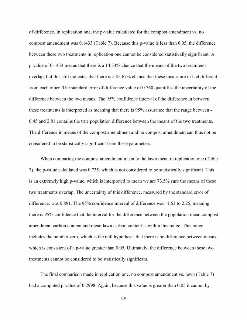
64

of difference. In replication one, the p-value calculated for the compost amendment vs. no

compost amendment was 0.1433 (Table 7). Because this p-value is less than 0.05, the difference

between these two treatments in replication one cannot be considered statistically significant. A

p-value of 0.1433 means that there is a 14.33% chance that the means of the two treatments

overlap, but this still indicates that there is a 85.67% chance that these means are in fact different

from each other. The standard error of difference value of 0.760 quantifies the uncertainty of the

difference between the two means. The 95% confidence interval of the difference in between

these treatments is interpreted as meaning that there is 95% assurance that the range between -

0.45 and 2.81 contains the true population difference between the means of the two treatments.

The difference in means of the compost amendment and no compost amendment can thus not be

considered to be statistically significant from these parameters.

When comparing the compost amendment mean to the lawn mean in replication one (Table

7), the p-value calculated was 0.735, which is not considered to be statistically significant. This

is an extremely high p-value, which is interpreted to mean we are 73.5% sure the means of these

two treatments overlap. The uncertainty of this difference, measured by the standard error of

difference, was 0.891. The 95% confidence interval of difference was -1.63 to 2.25, meaning

there is 95% confidence that the interval for the difference between the population mean compost

amendment carbon content and mean lawn carbon content is within this range. This range

includes the number zero, which is the null hypothesis that there is no difference between means,

which is consistent of a p-value greater than 0.05. Ultimately, the difference between these two

treatments cannot be considered to be statistically significant.

The final comparison made in replication one, no compost amendment vs. lawn (Table 7)

had a computed p-value of 0.2998. Again, because this value is greater than 0.05 it cannot by

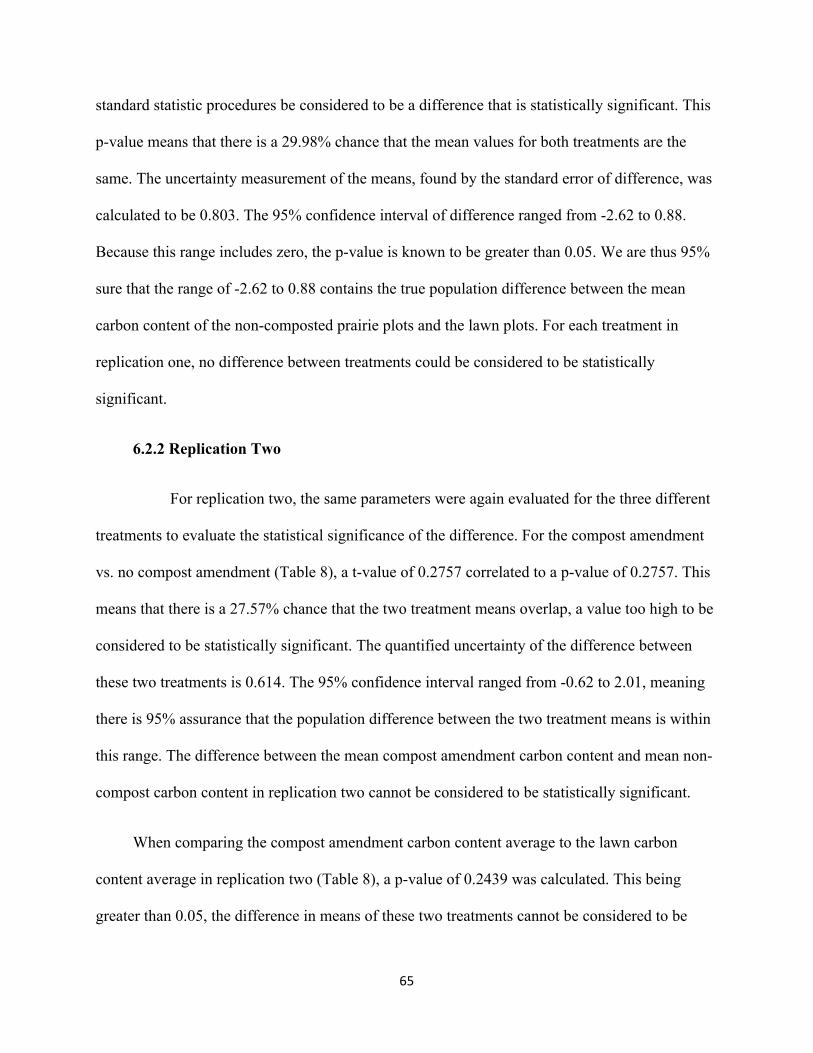
65

standard statistic procedures be considered to be a difference that is statistically significant. This

p-value means that there is a 29.98% chance that the mean values for both treatments are the

same. The uncertainty measurement of the means, found by the standard error of difference, was

calculated to be 0.803. The 95% confidence interval of difference ranged from -2.62 to 0.88.

Because this range includes zero, the p-value is known to be greater than 0.05. We are thus 95%

sure that the range of -2.62 to 0.88 contains the true population difference between the mean

carbon content of the non-composted prairie plots and the lawn plots. For each treatment in

replication one, no difference between treatments could be considered to be statistically

significant.

6.2.2 Replication Two

For replication two, the same parameters were again evaluated for the three different

treatments to evaluate the statistical significance of the difference. For the compost amendment

vs. no compost amendment (Table 8), a t-value of 0.2757 correlated to a p-value of 0.2757. This

means that there is a 27.57% chance that the two treatment means overlap, a value too high to be

considered to be statistically significant. The quantified uncertainty of the difference between

these two treatments is 0.614. The 95% confidence interval ranged from -0.62 to 2.01, meaning

there is 95% assurance that the population difference between the two treatment means is within

this range. The difference between the mean compost amendment carbon content and mean non-

compost carbon content in replication two cannot be considered to be statistically significant.

When comparing the compost amendment carbon content average to the lawn carbon

content average in replication two (Table 8), a p-value of 0.2439 was calculated. This being

greater than 0.05, the difference in means of these two treatments cannot be considered to be

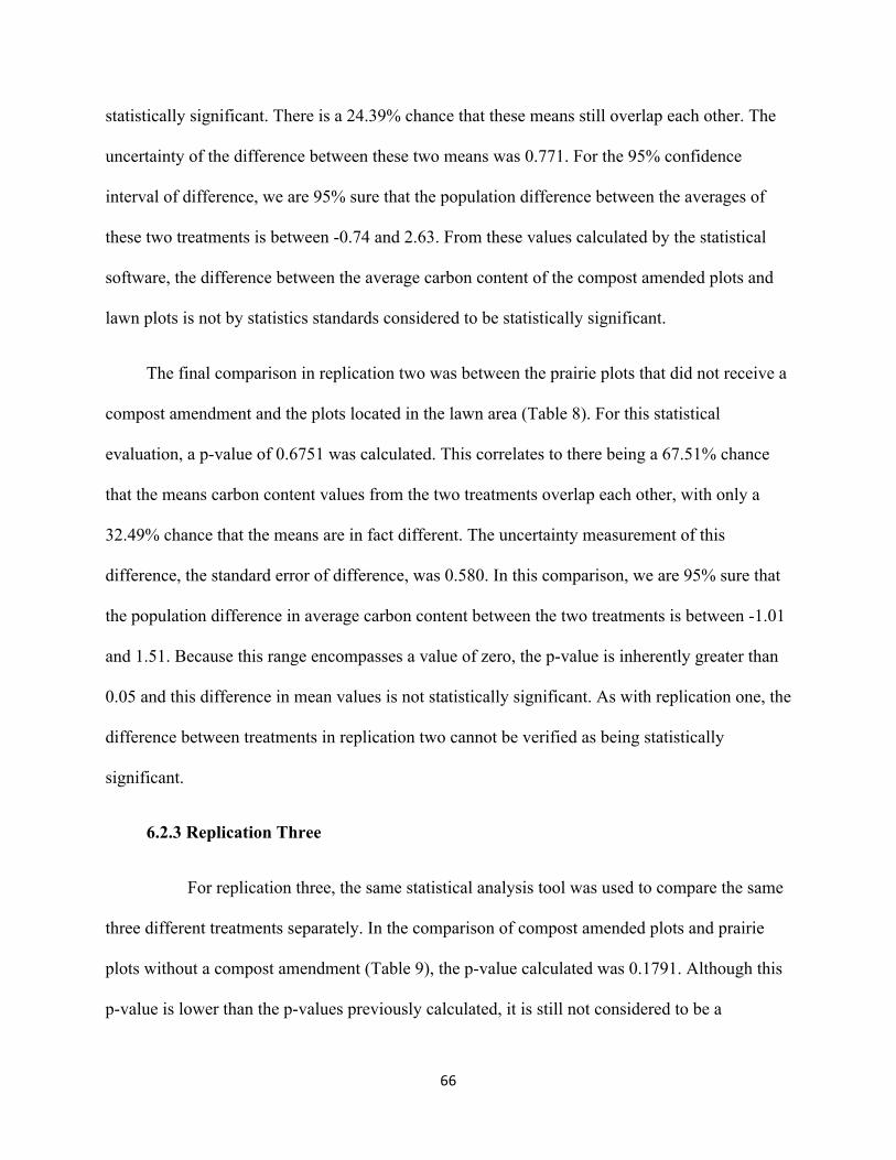
66

statistically significant. There is a 24.39% chance that these means still overlap each other. The

uncertainty of the difference between these two means was 0.771. For the 95% confidence

interval of difference, we are 95% sure that the population difference between the averages of

these two treatments is between -0.74 and 2.63. From these values calculated by the statistical

software, the difference between the average carbon content of the compost amended plots and

lawn plots is not by statistics standards considered to be statistically significant.

The final comparison in replication two was between the prairie plots that did not receive a

compost amendment and the plots located in the lawn area (Table 8). For this statistical

evaluation, a p-value of 0.6751 was calculated. This correlates to there being a 67.51% chance

that the means carbon content values from the two treatments overlap each other, with only a

32.49% chance that the means are in fact different. The uncertainty measurement of this

difference, the standard error of difference, was 0.580. In this comparison, we are 95% sure that

the population difference in average carbon content between the two treatments is between -1.01

and 1.51. Because this range encompasses a value of zero, the p-value is inherently greater than

0.05 and this difference in mean values is not statistically significant. As with replication one, the

difference between treatments in replication two cannot be verified as being statistically

significant.

6.2.3 Replication Three

For replication three, the same statistical analysis tool was used to compare the same

three different treatments separately. In the comparison of compost amended plots and prairie

plots without a compost amendment (Table 9), the p-value calculated was 0.1791. Although this

p-value is lower than the p-values previously calculated, it is still not considered to be a

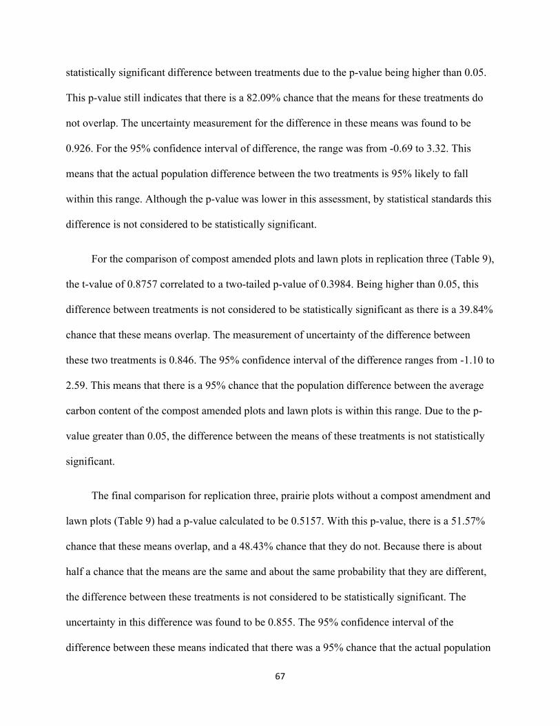
67

statistically significant difference between treatments due to the p-value being higher than 0.05.

This p-value still indicates that there is a 82.09% chance that the means for these treatments do

not overlap. The uncertainty measurement for the difference in these means was found to be

0.926. For the 95% confidence interval of difference, the range was from -0.69 to 3.32. This

means that the actual population difference between the two treatments is 95% likely to fall

within this range. Although the p-value was lower in this assessment, by statistical standards this

difference is not considered to be statistically significant.

For the comparison of compost amended plots and lawn plots in replication three (Table 9),

the t-value of 0.8757 correlated to a two-tailed p-value of 0.3984. Being higher than 0.05, this

difference between treatments is not considered to be statistically significant as there is a 39.84%

chance that these means overlap. The measurement of uncertainty of the difference between

these two treatments is 0.846. The 95% confidence interval of the difference ranges from -1.10 to

2.59. This means that there is a 95% chance that the population difference between the average

carbon content of the compost amended plots and lawn plots is within this range. Due to the p-

value greater than 0.05, the difference between the means of these treatments is not statistically

significant.

The final comparison for replication three, prairie plots without a compost amendment and

lawn plots (Table 9) had a p-value calculated to be 0.5157. With this p-value, there is a 51.57%

chance that these means overlap, and a 48.43% chance that they do not. Because there is about

half a chance that the means are the same and about the same probability that they are different,

the difference between these treatments is not considered to be statistically significant. The

uncertainty in this difference was found to be 0.855. The 95% confidence interval of the

difference between these means indicated that there was a 95% chance that the actual population

68

difference of these two treatments is between -2.45 and 1.31. Ultimately, the difference between

these two treatments is not great enough to be statistically significant.

6.2.4 Replication Four

In the final replication, the same procedure was followed to statistically analyze the

difference between treatments. For the compost amended plots and prairie plots without a

compost amendment (Table 10), the p-value calculated was 0.0084. This value is significantly

lower than 0.05, and this difference is thus considered to be highly statistically significant. We

could thus reject the null hypothesis that there was no difference between these two means. The

uncertainty in the difference calculation was found to be 0.464. For the 95% confidence interval

of the difference, the values ranged from 0.44 to 2.44. This range does not include the value zero,

agreeing with the determination that the p-value is less than 0.05. This was the only difference

between treatments in this experiment found to be statistically significant. This indicates that in

replication four, the difference between the average carbon content of the plots in the prairie that

received a compost amendment and the prairie plots without a compost amendment were

statistically significant. This is the only statistically significant indication in this experiment that

the compost amendment considerably boosted to carbon sequestration to an extent that created a

difference between treatments to be statistically significant.

For the comparison of the compost amended plots and the lawn plots in replication four

(Table 10), the calculated p-value was 0.0727. This value is extremely close to being under 0.05,

but is just shy of being low enough to declare the difference between means to be statistically

significant. This value still indicates that there is a 92.73% chance that there is a difference

between the two means. The uncertainty in the difference calculation between these treatments

69

was 0.547. The 95% confidence interval of difference was -0.12 to 2.29, meaning that we are

95% sure that this range contains the true population value of the difference between the two

treatments. While the p-value for these two treatments was still very low, by conventional

statistical standards the difference between treatments is not statistically significant.

The final statistical comparison made for this data consisting of comparing the mean

carbon content of the prairie plots without a compost amendment to the mean carbon content of

the lawn plots in replication four (Table 10). For this comparison, the p-value calculated was

0.461. This p-value is much larger than the necessary p-value of 0.05 to conclude that the

difference is statistically significant. Because there is a 46.1% chance that the means of these

treatments overlap, this difference is not considered to be statistically significant. The standard

error of difference calculation for this comparison was 0.467. Finally, the 95% confidence

interval of the difference was between -1.37 and 0.66. This indicates that there is 95% certainty

that the true population difference between these treatment carbon content averages is between -

1.37 and 0.66. This difference ultimately cannot be considered to be statistically significant.

6.2.5 Time Restraint

While the overall deduction of the statistical analysis is that the difference in carbon

content of the soil between treatments is not statistically significant, it is predicted that this

difference will become more apparent over time. The period between compost application and

soil testing was approximately six months, as compared to the three-year period that elapsed in

the Marin Carbon Project 10. While a three-year period was not plausible for the purposes of this

project, it would have more closely aligned with the procedure implemented in the Marin Carbon

Project. It is predicted that as more time passes between the compost application to the hillside,

70

the difference between treatments will become more apparent, potentially altering the statistical

analysis such that these differences are considered to be statistically significant. With greater

statistical significance in the impact that a single compost amendment has, the results of this

study can more closely aligned with those from Marin Carbon Project. It is possible that within

this six-month period between compost application and soil sampling, weather conditions or

outside factors impacted the ability of the soil to more significantly sequester carbon from the

atmosphere. As more time elapses, the organic matter implemented into the soil can stabilize and

continually be boosted due to the enhanced plant growth from the compost amendment. A

continuation of this experiment will determine whether a longer period of time will generate

statistically significant differences in soil carbon content between the different treatments.

6.3 Waypoint Analytical Soil Characteristics Interpretation

The Waypoint Analytical laboratory solely analyzed the soil samples collected from

the students in the ISAT 320 Fall 2015 class, as part of the laboratory procedure for this class.

The separate samples collected to the intent of this experiment were only analyzed in the on-

campus environmental lab rather than being sent to Waypoint Analytical. The samples collected

by the students in the ISAT 320 lab were taken from each of the same 10 x 10 meter plots that

were the soil site locations for this study as well. The soil depth at which students collected

samples was not consistent, either being too shallow or deep of a depth. As a result, separate

holes for sample collection were dug for the intent of this experiment. There is thus uncertainty

in the data provided from Waypoint Analytical because the sample depth was not consistent for

each plot. Flawed sampling procedures also create instability when comparing the Waypoint

Analytical results to the results obtained in this experiment. The prominent issue with

inconsistent sampling depths from the student samples is that the soil characteristic data could be

71

inaccurate because the soil sample did not incorporate an appropriate soil profile depth. Lastly,

because the exact soil sample location within the 10 x 10 meter plots differed between student

samples and personal samples, it is possible that differences between Waypoint data and data

from this experiment contrast due to the spatial difference.

While Waypoint Analytical provided data for multiple soil characteristics, only the organic

matter percentage (Table 11), phosphorous content (Table 13), and cation exchange capacity

(Table 12) were incorporated into this study. For the organic matter content of the soil samples,

Waypoint Analytical did not convert this into an estimation of the carbon content. Because it is

likely that the laboratory also used an alternate procedure than the one used in this study, the

results from Waypoint cannot be directly compared to those found in this experiment. Instead,

the overall trends between treatments will be compared to those found from this study. For the

plots that received a compost amendment, the average organic matter percentage calculated from

the Waypoint data was (6.8 +/- 1.753) percent (Table 14). The plots located in the prairie that did

not receive a compost amendment had an average organic matter percentage of (5.038 +/- 1.257)

percent (Table 14). Lastly, the lawn plots had an average organic matter content of (5.833 +/-

0.784) percent (Table 14). As observed from the data obtained through this study, the same trend

is present that the composted plots have the highest average organic matter content. As also seen

in previous results from this study, the lawn plots have the second highest average organic matter

content and the prairie plots without a compost amendment have the lowest average percentage

of organic matter.

The cation exchange capacity was next assessed (Table 12), which assesses the soil’s

capacity to retain cation nutrients important for plant growth. Following a composted organic

matter amendment, it was predicted that the cation exchange capacity would increase to indicate

72

that there was a higher availability of mineral nutrients available to the plant because the soil was

capable of retaining these. This relates back to the previously mentioned mycorrhizae, which

improves the plant uptake of water and mineral nutrients by the fungal hyphae. The average

cation exchange capacity measurement of the plots that received a single compost amendment

was (13.475 +/- 2.5138) meg/100g (Table 14). For the prairie plots without a compost

amendment, the average cation exchange capacity was (13.213 +/- 8.4019) meg/100g (Table 14).

While this value values close to that of the composted prairie plots, the prairie plots without a

compost amendment have a much higher standard deviation of 8.4019, indicating that there is

uncertainty that was introduced within this measurement. Lastly, the lawn plots had the highest

average cation exchange capacity measurement of (14.50 +/- 5.8570) meg/100g (Table 14). This

indicates that the lawn plots have, on average, the greatest potential to store cations within the

soil. While it would be expected that the prairie plots would have a higher cation exchange

capacity due to the abundance of plants, the lawn has a high root abundance, which explains why

these plots had a higher cation exchange capacity measurement. Uncertainty within the cation

exchange capacity of the soils can be attributed to the different composition of the soil samples

in regard to their percent composition of sand, silt, and clay. Soil with higher proportions of clay

and organic matter will have greater negative charge, meaning they will attract the positively

charged particles, or cations [14]. Soil samples with high amounts of organic matter and clay will

thus have a higher cation exchange capacity, and it is hard to decipher if this ability to retain

nutrients is due to organic matter or clay. Incorporation of soil composition in future studies

would assist in deciphering where exactly the large cation exchange capacity measurement is

rooted.

The last aspect of the data provided by Waypoint Analytical was the phosphorous content

73

of the soil. Because it was predicted that the composted organic matter amendment would

enhance the activity of the fungi, bacteria, and soil microorganisms underground, it was also

assumed that this amendment would thus enhance the availability of phosphorous within the soil.

The soil microorganisms, specifically bacteria, are able to solubilize inorganic phosphorous to

make it readily available for uptake by plants. As part of this holistic approach to analyzing the

soil health after a compost amendment, the ability of the soil microorganisms to facilitate the

availability of phosphorous for plants was incorporated into this study. The prairie plots that

received a single compost amendment had an average phosphorous concentration of (125.50 +/-

48.893) ppm (Table 14). This measurement was associated with a high standard deviation of

48.893 ppm, indicating that there was variation between treatment plots and possible uncertainty

introduced into measurements. The prairie plots that did not receive a compost amendment had

an average phosphorous concentration of (46.25 +/- 28.019) ppm (Table 14). Again, there is high

variation amongst the plots due to this elevated standard deviation measurement. Lastly, the lawn

plots had an average phosphorous content of (70.50 +/- 21.427) ppm (Table 14). The standard

deviation of this measurement is lower, but still relatively high in comparison to the average

phosphorous measured. The compost amended prairie plots by far had the highest concentration

of phosphorous in the soil, indicating that there were possibly more soil microorganisms present

or there was a higher amount of phosphorous being solubilized due to the activated soil microbes

following the organic matter amendment. The composted plots had the highest availability of

phosphorous, meaning the plants in these plots had greater access to this macronutrient.

74

6.4 Waypoint Analytical Statistical Analysis Interpretation

6.4.1 Organic Matter Percentage

To assess the statistical significance between treatments from the Waypoint

Analytical data, an unpaired two-tailed t-test was again used from the same GraphPad Statistical

Software. The same parameters previously studied were again analyzed for the Waypoint data.

The statistical analysis done for the Waypoint data was with the organic matter percent measured

across the three different treatments. When comparing the compost amended plots to the prairie

plots without a compost amendment (Table 15), a p-value of 0.0365 was calculated. This p-value

is less than 0.05, meaning it can be concluded that the difference in organic matter content

between composted and non-composted plots is statistically significant. The uncertainty in this

difference measurement, calculated by the standard error of difference, was 0.763. The 95%

confidence interval of the difference ranged from 0.13 to 3.40. Because this range does not

contain the value zero, the null hypothesis that there was no difference in the mean organic

matter content between these two treatments is thus rejected. As found in replication four from

this experiment, the difference in organic matter content between the composted plots and prairie

plots that did not receive a compost amendment is considered to be statistically significant. This

agrees with the originally stated hypothesis that a single compost amendment would boost the

carbon sequestration, and thus the organic matter content of the soil.

Next, the compost-amended prairie plots were compared to the lawn plots to analyze the

difference in average organic matter content (Table 15). The calculated p-value for this

comparison was 0.2348, meaning that there is a 23.48% chance that the organic matter averages

between these two treatments overlap. Being that this percentage is greater than 5%, the

75

difference in organic matter content between the compost amended plots and lawn plots was not

statistically significant. The uncertainty in this measure of difference for this comparison of

treatments was 0.773. Finally, the 95% confidence interval of difference ranged from -0.72 to

2.65, meaning that the actual population difference between these treatments is within this range.

Because the p-value is greater than 0.05, we failed to reject the null hypothesis that there is no

difference between means. The difference in organic matter content of the compost amended

prairie plots and lawn plots is thus not statistically significant.

The average organic matter content of the prairie plots without a compost amendedment

was then compared to the average organic matter content of the lawn plots (Table 15). The p-

value for this comparison was 0.1995, which is higher than 0.05 and is thus not a statistically

significant difference. An 80.05% still exists that there is a difference in the average organic

matter percentage between the non-composted amended prairie plots and the lawn plots. The

uncertainty in this measurement of difference between treatments is 0.586. The 95% confidence

interval of difference indicates that the actual average population difference between the non-

composted prairie plots and lawn plots is between -2.03 and 0.48. Because this confidence

interval of difference contains the number zero, we fail to reject the null hypothesis that there is

no difference between the average organic matter content of these treatments.

6.4.2 Cation Exchange Capacity

The next statistical analysis was to compare the cation exchange capacity

differences between treatments. The compost amended prairie plots were foremost compared to

the non-composted prairie plots (Table 16). The p-value for this comparison was 0.9337, an

extremely high p-value that indicates that the difference between treatments is not statistically

76

significant. There is only a 6.63% chance that the means for these two treatments do not overlap,

which is extremely low. The uncertainty of the measurement of difference for this replication

was 3.101. The 95% confidence interval of the difference was -6.39 to 6.91. This means that the

true difference of the population means between these treatments is within this range. The

difference in average cation exchange capacity between the compost amended plots and non-

composted prairie plots was not statistically significant.

The cation exchange capacity differences between the compost amended plots and lawn

plots was next compared (Table 16). The p-value from the two-tailed t-test between these two

treatments was 0.6624, which is significantly greater than the necessary p-value of 0.05 to

conclude that the difference is statistically significant. A p-value of 0.6624 indicates that there is

only a 33.76% chance that the means of these two treatments no not overlap. The measurement

of uncertainty in the difference between these two treatments was 2.29. The confidence interval

of the difference indicated that there was 95% certainty that the true population mean differences

between these two treatments was between -6.01 and 3.96. Because this confidence interval

contains the number zero, we failed to reject the null hypothesis that there was no difference in

the average cation exchange capacity between the compost amended plots and the plots located

in the lawn area.

The final comparison made for the cation exchange capacity averages was between the

non-composted prairie plots and the lawn plots (Table 16). For this statistical analysis, a p-value

of 0.7544 was found. This p-value signifies that there is a 75.44% chance that the mean cation

exchange capacity of the non-composted prairie plots and lawn plots overlap, which greatly

exceeds the necessary 5% value to conclude that the difference in mean values is statistically

significant. The uncertainty measurement of this difference calculation is 4.022. The 95%

77

confidence interval calculated by the statistical software produced a range of values from -10.05

to 7.48. This means that the true difference in population cation exchange capacity averages is

within this range, which is a range with a relatively large span of values. The difference between

average cation exchange capacity between non-composted prairie plots and lawn plots is not

statistically significant, and there is a considerable amount of uncertainty within this statistical

calculation.

6.4.3 Phosphorous Concentration

The final statistical analysis executed for the Waypoint data was with the

phosphorous content found from the soil samples. The phosphorous content between the

compost amended plots and non-composted prairie plots (Table 17) was the first comparison

executed in this section. The p-value calculated in this statistical analysis was 0.0014, which is

an extremely low value indicating the difference in phosphorous content between these two

treatments was very highly statistically significant. There is only a 0.14% chance that the

averages in phosphorous content of these different treatments overlap. This indicates the

compost amended plots have a notably higher content of phosphorous available for plants to

consume. The uncertainty of the difference, the standard error of difference, was calculated to be

19.924. The 95% confidence interval of the difference in phosphorous content ranged from 36.52

to 121.98. This means that there is 95% certainty that the actual population difference between

average phosphorous content between compost amended and control plots is within this range.

From this statistical analysis, the null hypothesis that there is no difference between the means is

rejected, as this difference in phosphorous concentration between treatments is considered to be

statistically significant.

78

Next, the phosphorous concentration of the compost amended plots and lawn plots was

compared (Table 17) with the statistical software. The two-tailed p-value produced was 0.0251, a

value lower than the value of 0.05 needed to verify that the difference is statistically significant.

Again, because the composted plots had such a drastically high concentration of phosphorous in

comparison to the other treatments, the null hypothesis that there is no difference between the

mean phosphorous concentration of composted plots and lawn plots is rejected. The

measurement of uncertainty in the differences between treatments was found to be 21.506. The

95% confidence interval of the difference ranged from 8.14 to 101.86, which is a range with an

extremely wide span. This wide span originates from the high standard deviation values that

were found when evaluating the phosphorous content within specific treatments (Table 14). The

diversity in plant density and species across the hillside likely affected the phosphorous

concentration spatially, which explains why there is such high uncertainty in the measurement of

phosphorous. Although there is uncertainty within the statistical analysis, it is still concluded that

the difference in phosphorous concentration between composted plots and lawn plots is

statistically significant.

The final statistical analysis evaluated the difference in phosphorous concentration

between prairie plots without a compost amendment and the lawn plots (Table 17). The

statistical software calculated a p-value of 0.1035, a value slightly too high for the differences

between these treatments to be considered statistically significant. The p-value still indicates that

there is a 89.65% chance that the two means being evaluated do not overlap each other, but a

95% chance is necessary to conclude that the difference is statistically significant. The

measurement of uncertainty calculated in this statistical analysis of difference between means is

13.761. The 95% confidence interval was interpreted such that the actual difference in

79

population means is between -54.23 and 5.73. Again the span of this range is extremely wide,

which is a result in the large standard deviations found for the phosphorous concentrations.

Ultimately, the difference in average phosphorous concentration between non-composted prairie

plots and lawn plots is not considered to be statistically significant, and thus we fail to reject the

null hypothesis that there is no difference between means.

6.5 Data Omitted

Aside from the predominant areas of uncertainty in the study that affected the carbon

content and soil characteristics measured, there were additional areas to be addressed that

introduced uncertainty during the investigation of results. The first being an outlier encountered

in replication three of the soil carbon content investigation (Table 4). The carbon percentage

measured from soil sample S1G1 was found to be 0.37, which is an extremely low value that

would indicate there is organic matter content of the soil is nearly absent. This outlier was not

included in the average soil carbon content calculations made in this study (Table 6) because it

would offset the interpretation of soil carbon content. The value was also omitted in the

statistical analysis executed for replication three results (Table 9). Although this value was

rejected from the mathematical calculations completed in this study, the value was still displayed

on the ArcGIS visualization of the results (Figure 10). This outlier is likely due to human error

during the laboratory procedure for finding the carbon content of soil samples. The unusually

low carbon percentage could also be attributed to fault in the scale being used in this experiment.

A low carbon percentage calculation denotes that there was an extremely small difference in the

weight of the sample before and after the sample was burned at 700°C. Because this small of a

value was not observed in any other soil samples, this specific result was considered an outlier in

this study that did not accurately represent the soil carbon content of the particular sample.

80

Another issue addressed in this experiment was an insignificant amount of soil for the

carbon content evaluation. Because the soil samples were collected in the Fall 2015 semester and

weren’t analyzed until the muffle furnace was available in the Spring 2016 semester, the soil

analyzed was limited to the amount originally collected. Due to the variation observed in carbon

content between replications and within treatments, more replications were completed than

originally intended. By replication four, the amount of soil left was extremely limited, and soil

sample S4G4 was unable to be analyzed (Table 5) because it had been expended after the third

replication. As a result, the mathematical calculations performed during this experiment had to

exclude this sample (Table 6). The statistical analysis executed for each replication also excluded

this soil sample (Table 10), and fewer samples in a statistical analysis generate a weaker

statistical analysis. This particular sample was also absent in the ArcGIS visualization of results

(Figure 11). To avoid this issue in future work, it is recommended that researchers collect

samples with a greater volume of soil to thwart a deficiency of soil to be analyzed.

81

Chapter 7 Conclusion

The results of this study indicate that based on average soil carbon content, the plots that

received a singular composted organic matter amendment had the highest percentage of carbon

stored within the soil. The composted plots had an average carbon percentage of (5.81 +/- 1.67)

(Table 6), compared to an average carbon percentage of (4.49 +/- 1.72) (Table 6) within the

control prairie plots that did receive a compost amendment. The composted plots had in increase

in carbon sequestration that resulted in over a 1% difference in carbon content than the non-

composted control plots located in the prairie. After only six months between compost

application and soil sampling, this difference in carbon content between the composted and non-

composted plots is significant and indicates that the compost amendment successfully boosted

the capture and sequestration process of carbon by the plants on the hillside.

The average carbon percentage of the plots located in the lawn was (5.02 +/- 1.42) (Table

6), which was higher than the average carbon content of the non-composted prairie plots due to

the high root abundance of the grass area. The composted plots had slightly less than a 1%

increase in carbon content compared to the plots in the grass area. Because the grass area plots

served as a comparison between the naturalization hillside and managed grass area, the results

indicate that a composted, natural prairie can enhance the carbon sequestration within the soil.

To heighten soil carbon sequestration, optimal conditions consist of a naturalized prairie with the

addition of a single compost amendment consisting of organic matter. Implementing this land

amendment assists in offsetting carbon dioxide emissions being emitted into the atmosphere

from fossil fuel burning for energy resources. Composted organic matter amendments to the soil

provide a natural, efficient, cost-effective, and immediate solution to the saturation of carbon

dioxide emissions in the atmosphere.

82

While differences between treatments were observed in terms of average carbon content

percentage, these distinctions were not considered to be statistically significant according to

conventional statistical criteria. The only statistically significant difference in average carbon

content was found in replication four between the compost amended plots and non-composted

prairie plots (Table 10). Aside from this single indication of statistical significance in the

difference between treatments, statistical analysis did not indicate that the carbon content of soils

was significantly altered following a compost amendment. It is predicted that as more time

elapses after the single compost amendment, this difference between treatments will become

more apparent and statistically significant. To align with the timeline of the Marin Carbon

Project, the carbon content of the soils should be evaluated for at least a three-year period to

observe the development of carbon content within the soil. While the difference in carbon

percentage of the hillside between treatments is not currently statistically significant, it is

probable that as more time elapses, these differences will become statistically significant and

align more closely with the results obtained by the Marin Carbon Project.

There was a high level of variation within the data obtained throughout this study, both

between replications and within the different treatment results. While uncertainty is unavoidable,

these avenues were identified so that in future work the influence it has on the results can be

minimized. Possible areas of uncertainty in this study included the soil mixing procedure that

was altered after replication two, the high root abundance present within the soil samples, the

shallow and rocky conditions of the soil, compaction from the previous dirt road, faulty

measurement devices, and human error. By identifying the channels by which uncertainty affects

the data, more variables can be included in future work that attempt to quantify this uncertainty

and address the degree to which it offsets the data. Being that this was the first year of this study

83

on the hillside, the project was investigative and nature and the sources of uncertainty were not

previously identified. Completion of this experiment and data assessment will potentially

alleviate some areas of uncertainty and error in the data with future experiments concerning

carbon sequestration on the hillside.

Aside from the boost in average carbon content of the soil, Waypoint Analytical data

indicated that there were additional benefits acquired by the soil following the organic matter

amendment. The average phosphorous content of the compost-amended plots was (125.50 +/-

48.893) ppm (Table 14), in comparison to the control prairie plots that had an average

phosphorous concentration of (46.250 +/- 28.019) ppm (Table 14). The phosphorous average of

the lawn plots, (70.50 +/- 21.427) ppm (Table 14), was also higher than that of the control plots.

The average phosphorous content of the compost-amended plots was statistically significantly

different from the non-composted control plots and lawn plots (Table 17), indicating that there

was a higher availability of phosphorous for uptake by plants following the organic matter

amendment. Because phosphorous is a macronutrient, a greater amount of phosphorous present

in the soil reduces the need for fertilizer application to sustain plant growth. Although there was

high variability in phosphorous measurements made between the designated plots, the

application of organic matter significantly increased the availability of phosphorous to plants

such that plant growth could be boosted and carbon sequestration could be facilitated.

Statistical analysis of the cation exchange capacity data from Waypoint Analytical

indicated that the difference between treatments was not statistically significant (Table 16). The

cation exchange capacity remained relatively uniform across treatments (Table 14), which agrees

with the data from this experiment that there wasn’t a statistically significant difference between

average carbon content of treatments. An increase in organic matter content or clay content

84

would boost the cation exchange capacity of soil due to their negative charge. Without a

statistically significant difference in carbon content of composted and non-composted plots, the

cation exchange capacity of the soil would not be considerably altered. As with the average

carbon content of the soil on the hillside, it is predicted that as a greater amount of time passes

after the compost amendment, the difference in cation exchange capacity of the soil will become

more prominent. It is projected that the cation exchange capacity of the composted plots will

intensify more greatly than that of the control prairie plots. By introducing a study of the soil

composition into future work, differences in cation exchange capacity can be attributed more

clearly to either a high content of clay or organic matter.

The organic matter content calculated by Waypoint Analytical (Table 14) indicated that

the average organic matter content percentage the composted plots, (6.80 +/- 1.753), was more

than 2% higher than the non-composted control plots. This average organic matter percentage

was also nearly 1% higher than the average organic matter percentage of the lawn plots. The

difference between the composted plots and non-composted prairie plots (Table 15) was by

conventional standards, considered to be statistically significant. This is in unison with the

statistical analysis conducted for replication four (Table 10), meaning that there is indication

from both this experiment and Waypoint Analytical that the compost amendment to the hillside

enhanced the soil carbon sequestration. While there is variation amongst the data obtained from

this experiment and Waypoint Analytical, as time elapses and sources of uncertainty are

addressed, the difference between treatments is predicted to become more apparent as it did in

the Marin Carbon Project following a three-year analysis 10.

The definitive conclusion reached in this study is that a singular compost amendment can

serve as an effective land management technique for boosting the average carbon percentage of

85

the soil. To determine the long-term effects of a compost amendment, studies must be

maintained that analyze the trend of carbon content within the soil. The results of this experiment

indicate that there is upward trend of carbon sequestration on the composted plots, but the

difference in soil carbon content between various treatments is not yet statistically significant.

With a greater lapse of time between compost amendment and soil sampling, it is predicted that

the difference in soil carbon percentage between treatments will become more evident and thus

statistically significant. Multiple areas of uncertainty were identified in this study, and it is

recommended that future studies incorporate an analysis of these sources of uncertainty so the

degree to which they affect the output data can potentially be quantified and minimized.

86

Chapter 8 Future Work

This experiment was modeled after the ongoing Marin Carbon Project, which is currently

an ongoing study being executed that was initiated in 2008. The research experiment conduced

on the ISAT Hillside was started in March of 2015. The time elapsed between the compost

application and soil testing under the Marin Carbon Project was roughly three years [10]. Because

the period between the compost amendment application and the soil sampling was about six

months, this experiment requires greater time and research to follow the timeline of the Marin

Carbon Project. This experiment will be continued under the direction of Dr. Wayne Teel to

determine if the difference between treatments on the Hillside becomes more apparent over time.

Continuation of this experiment will allow researchers to conclude if a greater portion of time

between the organic matter amendment application and soil testing accounts for a more

observable difference between the composted and non-composted plots. The difference in

average carbon content between treatments in this experiment could not be concluded to be

statistically significant. With a greater time lapse, it is possible that the difference in soil carbon

content between treatments will intensify and thus be considered statistically significant.

In this experiment, there were a number of factors that introduced uncertainty within the

data. Soil samples collected often harbored a high root abundance, which alters the weight

differences during the burning process. During future work, a more accurate depiction of the soil

carbon content can be obtained if a procedure is implemented to remove the root biomass found

in soil samples. The sieve shaker mixing technique must be utilized before each replication to

ensure the same procedure is being implemented across all replications. An identical procedure

for each replication allows the results from each replication to be more appropriately compared.

Using a smaller sieve size could potentially remove the abundance of roots within soil samples,

87

and if this method fails it is recommended that root fragments be manually removed from the soil

sample. Research into procedures for removing root biomass from soil samples would provide

researchers with background data and past procedures that were implemented to account for this

issue.

Another area of ambiguity within this study is the complication that occurred when

collecting soil samples. Due to the shallow and rocky properties of the sample locations, a depth

of approximately six inches was utilized when collecting samples. This was the maximum depth

obtainable with the equipment used, and soil samples were frequently littered with a large

portion of rocks. An ideal sample depth for this study type is eight inches, which is greater than

the soil depth obtained in this experiment. A new sampling technique or equipment could

overcome the soil sampling difficulties and allow future studies to analyze soil from a depth of

eight inches. Enhancing this sampling technique will allow this study to more closely follow

previous studies investigating soil organic matter. A sample depth of at least eight inches will

additionally grant the researchers with a more accurate depiction of the soil characteristics.

The study site in this experiment previously had a dirt road running parallel to the prairie

strips. When the land was purchased by James Madison University, the maintenance department

simply planted over the old dirt road. The presence of this road is likely to have highly

compacted the soil that it ran over, making it more difficult for vegetation roots to penetrate into

the ground. While soil compaction is analyzed in the ISAT 320 Lab, this soil characteristic was

not incorporated into this study. This study could be enhanced by delving into the soil

compaction on the sample site from the past road, and this factor could possibly contribute to the

analysis of carbon content found within the soil. When the carbon content of the plots was

88

spatially analyzed in ArcGIS, having the soil compaction background knowledge would provide

the researcher with a greater understanding of any discrepancies within the results.

Aside from recommendations for resolving uncertainties within this experiment,

additional study factors can be incorporated into the study to greater understand the effects of an

organic compost amendment. For future work concerning this experiment, it is recommended

that more samples be collected from each 10 x 10 meter plot to determine if there are spatial

differences in the soil carbon content amongst each plot. With more soil samples in total, more

samples can be analyzed in the lab to produce a greater volume of results. With more samples

analyzed and more replications, the statistical analysis becomes more representative of the

results. A greater amount of data reduces the occurrence of random error and generates results

that are more representative of the actual soil carbon content. To acquire more soil samples to be

analyzed, it is also recommended that a larger team be formed for future studies to make the soil

sampling and analyzing procedure simpler and more efficient.

To broaden the scope of this experiment, additional factors can be incorporated into the

study. The ISAT Hillside hosts a plethora of vegetation species, and it is possible that the

different plant species release carbon at different rates. Previous studies have indicated that

compost successfully boosts plant growth, and the extent of this outcome can be analyzed in this

study. By documenting the plant diversity and density on the Hillside, this can be compared

against the varying soil carbon content values calculated. The incorporation of plant studies into

this experiment introduces several variables and reactions to be analyzed. With boosted plant

diversity on the Hillside, it is likely that the soil would become more resilient due to enhanced

microbial life. With heightened microbial activity, the abundance of nutrients such as

phosphorous and nitrogen would likely increase surrounding the plants. A new procedure for

89

analyzing soil microbe activity would have to be researched and incorporated into this study to

allow future work to address the effect of plant species and microbial diversity. In addition, a

procedure would have to be implemented to allow researchers to calculate the amount of

different nutrients within the soil to connect these different variables. Again, a larger team would

make this process more feasible.

The cation exchange capacity of the soil was analyzed using the data provided by

Waypoint Analytical. Because organic matter and clay are both negatively charged, they attract

these cations, or positively charged particles. The organic amendment was predicted to boost the

cation exchange capacity of soil, meaning that the soil would be capable of retaining these

mineral nutrients as a source of nutrients for the plants growing. The soil composition was not

evaluated in this study, but would provide deeper insight into whether the differences in cation

exchange capacity between treatments was due to an abundance of clay particles or organic

matter. The cation exchange capacity affects the soil fertility, and thus is necessary to have a

high cation exchange capacity due to the presence of organic matter. Without a suitable cation

exchange capacity, the soil would be limited in nutrient availability, and would also be

inefficient storing these nutrients. Although an appropriate amount of clay is necessary to attract

and retain cations, an extremely high clay level would induce anaerobic conditions due to the

compaction of the soil and inability for air to exist. Soil can thus have a high cation exchange

capacity due to clay, but also have inhabitable conditions for soil microbes and plant growth.

There were soil samples collected in this study that were primarily composed of clay, but

because the soil composition was not evaluated in this study, it wasn’t possible to draw

connections between clay content and cation exchange capacity, In future studies, soil

90

composition should be determined so that any outliers of cation exchange capacity can be

analyzed and determined to either arise due to organic matter or clay content.

A final area of study that could be integrated into this experiment would be observing an

increase in water holding capacity of the soil. Past studies analyzing the effects of an organic

matter amendment have incorporated an analysis of the difference in the water holding capacity

of the soil. Too boost the extent of this research a procedure to measure the water holding

capacity could be replicated from past studies. It was concluded in this experiment that the

compost amendment increased the amount of soil aggregates within the soil, thus correlating to a

higher proportion of humus and carbon sequestered in the soil. It can then be predicted that with

an increase of soil aggregates, the soil becomes more “spongy” and capable of retaining water to

enhance soil health and reduce any runoff. Research is necessary to determine efficient means of

determining the water holding capacity of soil. Adding this aspect into the study would extend

the scope of the project beyond means by which the compost amendment reduces carbon dioxide

emissions in the atmosphere. It would thus serve to incorporate a greater understanding of the

boost in soil health that is correlated to an organic matter amendment.

91

Chapter 9 Unintended Consequences

Within this research project, there were possible areas for unintended consequences to be

introduced. A negative unintended consequence is the possible damage of aboveground

vegetation and belowground symbiotic relationships between plant roots and mycorrhizae.

Because the ISAT Hillside Naturalization Project consists of mowing evasion during the growing

season, the plants and grasses are unrestricted in terms of how large they can grow. When it was

time to collect soil samples, it was necessary to maneuver through the unhindered and

flourishing plants. To pinpoint the location for each sample site, a portion of the vegetation was

crumpled when traveling through the prairie. As a result, a fraction of the vegetation growth on

the prairie was stunted due to foot travel. Increased pedestrian traffic on the prairie from this

research experiment and the ISAT 320 class likely increased the soil compaction slightly and

damaged the growth of plants. In addition, when holes were the soil samples were collected from

were dug using an auger and trough shovel. Digging into the soil with these instruments breaks

up the formation of mycorrhizae underground due to the turning nature of the auger device.

Although care was taken not to disturb the aboveground vegetation and belowground root

formation, an unintended consequence of this study is that these variables are inherently affected

due to the invasive soil sampling technique and heavy foot traffic.

A possible unintended yet positive consequence of this study involves the potential for

this project to impact the landscape management techniques of JMU facilities. Boosted plant

growth and water holding capacity of the hillside following the compost application likely

enhances the hillside’s resistance to erosion and runoff. The decreased runoff in turn reduces the

amount of pollution entering the stream at the bottom of the hillside. The overall health of both

the hillside and stream are thus boosted following the compost amendment. While this was not

92

an area of study within this project, this lessens the burden for the university facilities

management to maintain the health of the hillside and stream because the water is naturally

filtered as retained in the soil as it travels down the hillside. Aside from the positive

environmental outcomes, this would also assist in reducing the cost of landscape and water

quality management.

Finally, an additional positive unintended consequence would be the reduction of food

waste stemming from James Madison University. Because the compost in this study was partly

composed of food waste from the university, the amount of food being deposited in landfills was

decreased. Gases emitted from landfills are about 50 percent methane and 50 percent carbon

dioxide and water vapor, as well as minute amounts of nitrogen, oxygen, hydrogen, nonmethane

organic compounds, and trace amounts of inorganic compounds [15]. By decreasing the

proportion of food being allocated towards landfills, this project has the unintended consequence

of decreasing the amount of landfill gases being emitted into the atmosphere. Not only is the

organic compost amendment directly offsetting atmospheric carbon dioxide emissions, but by

decreasing the volume of food being stored in landfills this project also has indirectly diminished

atmospheric pollution from landfills.

93

Bibliography

1. White, Courtney. Grass, Soil, Hope: A Journey through Carbon Country. White River

Junction, VT: Chelsea Green Publishing, 2014.

2. Ohlson, Kristin. The Soil Will Save Us: How Scientists, Farmers, and Foodies Are

Healing the Soil to Save the Planet. New York, NY: Rodale Inc., 2014.

3. United States Environmental Protection Agency. “Overview of Greenhouse Gases.”

United States Environmental Protection Agency. Accessed March 13, 2016.

https://www3.epa.gov/climatechange/ghgemissions/gases/co2.html

4. United States Environmental Protection Agency. “Causes of Climate Change.” United

States Environmental Protection Agency. Accessed March 13, 2016.

https://www3.epa.gov/climatechange/science/causes.html

5. Cabrera, V.E., Stavast, L.J., Baker, T.T., Wood, M.K., Cram, D.S., Flynn, R.P., Ulery,

A.L., 2009. Soil and runoff response to dairy manure application on New Mexico

rangeland. Agric. Ecosyst. Environ. 131, 255-262.

6. Eghball, B., Power, J.F., 1999. Composted and noncomposted manure application to

conventional and no-tillage systems: corn yield and nitrogen uptake. Agron. J.

91, 819-825.

7. Ryals, Rebecca, Melannie D. Hartman, William J. Parton, Marcia S. DeLonge, and

Whendee L. Silver. "Long‐term climate change mitigation potential with organic

matter management on grasslands." Ecological Applications 25, no. 2 (2015):

531-545.

8. Ryals, Rebecca, and Whendee L. Silver. "Effects of organic matter amendments on net

94

primary productivity and greenhouse gas emissions in annual

grasslands." Ecological Applications 23, no. 1 (2013): 46-59.

9. American Carbon Registry. “Methodology for Compost Additions to Grazed Grasslands”

The American Carbon Registry. October 2014. Accessed April 10, 2016.

http://americancarbonregistry.org/carbon-accounting/standards-

methodologies/methodology-for-greenhouse-gas-emission-reductions-from-

compost-additions-to-grazed-grasslands/compost-additions-to-grazed-grasslands-

v1-0_final-1.pdf

10. Marin Carbon Project. “Can Land Management Enhance Soil Carbon Sequestration?”

Marin Carbon Project. Accessed March 14, 2016.

http://www.marincarbonproject.org/science/land-management-carbon-

sequestration

11. Owen, Justine J., William J. Parton, and Whendee L. Silver. "Long‐term impacts of

manure amendments on carbon and greenhouse gas dynamics of

rangelands." Global change biology 21, no. 12 (2015): 4533-4547.

12. Lynch, D. H., R. P. Voroney, and P. R. Warman. "Soil physical properties and organic

matter fractions under forages receiving composts, manure or

fertilizer." Compost science & utilization 13, no. 4 (2005): 252-261.

13. U.S. Climate Data. “Climate Harrisonburg – Virginia.” U.S. Climate Data. Accessed

March 14, 2016.

http://www.usclimatedata.com/climate/harrisonburg/virginia/united-

states/usva1374/2016/3

14. Purdue University Cooperative Extension Service. “Fundamentals of Soil Cation

95

Exchange Capacity (CEC).” Purdue University. Accessed April 17, 2016.

https://www.extension.purdue.edu/extmedia/ay/ay-238.html

15. United States Environmental Protection Agency. “Landfill Gas.” United

States Environmental Protection Agency. Accessed April 18, 2016.

https://www3.epa.gov/lmop/faq/landfill-gas.html

compost land management and soil carbon sequestration

Documents