Component Shape Optimisation for Enhanced

Non-Destructive Testing

J. Singh1,∗, A. J. Mulholland2, K. M. M. Tant1, T. Stratoudaki1, A. Curtis3,

W. Ijomah1, J. F. C. Windmill1

1University of Strathclyde, Glasgow, UK

2Department of Engineering Mathematics, University of Bristol, UK

3School of Geosciences, University of Edinburgh, UK

∗Corresponding author: jonathan.singh@strath.ac.uk

August 6, 2020

Abstract

Determining an optimal component design is fundamental to many applications including

many of those in the aerospace, automotive and civil engineering industries. Previously, the

compatibility of the component with future non-destructive testing (NDT) requirements has

not been considered at the design stage. As a result, NDT operators are often challenged to

reliably inspect components with complex geometries. In this paper, a framework is proposed

for the optimisation of a component’s shape to maximise the sensitivity and coverage of an

interrogating ultrasonic wave, thus enhancing the ability to non-destructively image defects.

The design of beam cross-sections are optimised using both a low-dimensional parameterisation

with a genetic algorithm, and the level set method which enables more degrees of freedom in the

component shape parameterisation. Images of flaws computed using the total focusing method

show an 8 dB improvement in the signal to noise ratio for the optimised component as well as a

five-fold improvement in the estimate of flaw size. These results show that the NDT-optimised

design of components can provide significant improvements in flaw imaging. This in turn assists

in extending the lifespan of in-service components and indeed their remanufacturability, which

is both environmentally and economically advantageous.

Key words: Design, Shape optimisation, Level set method, Non-destructive testing, Ultrasound

1

brought to you by COREView metadata, citation and similar papers at core.ac.uk

provided by University of Strathclyde Institutional Repository

1 Introduction

The development of sustainable methods for the manufacture of components is critical across

all engineering disciplines. One environmentally friendly and economically viable approach is

remanufacturing ; the process of bringing a used product to a state that performs at least at the

same level as the original product, and is therefore issued an as-new warranty [19, 27].

The remanufacturing procedure is as follows: a product is stripped down to its individual com-

ponents; the components are cleaned, assessed, remanufactured and restored; then the product

is rebuilt and performance tested [19]. Lund [27] indicates that 85% of the mass of a reman-

ufactured product may be sourced from used components, and requires 50–80% less energy to

produce, providing a 20–80% production cost saving in comparison to conventional manufactur-

ing. The principle of design-for-remanufacturing (DfREM) recognises the importance of the initial

component design in aiding the steps involved in the remanufacturing process [15].

During the remanufacturing assessment stage, the detection of any internal defects is critical;

both production costs and environmental impact are reduced when the level and reliability of

inspection is enhanced, so that defective components are also not propagated through the manu-

facturing process. Non-destructive evaluation or testing (henceforth, NDT) is a term that describes

a range of methods that evaluate components non-invasively [38]. The dominant modality is ultra-

sonic NDT, which uses high-frequency mechanical waves to image the interior of a component [41].

These methods allow for inexpensive, near real-time, and high resolution images of a component’s

interior to be generated and any internal defects detected [6, 26], even in heterogeneous material

[46, 47, 48]. However, although reliable NDT is key for maintenance and life extension of a com-

ponent, the suitability of a component for NDT is not currently considered in the optimisation of

most component’s design [47].

In the last decade, ultrasonic NDT has seen a rapid increase in the use of ultrasonic phased ar-

rays for standardised inspection of components [20, 53]. The advantage of using arrays is increased

imaging quality as the array can control the directivity and focus of the ultrasound by varying the

time delay between firings of the array elements. However, in general, ultrasonic phased arrays are

based on piezoelectric transduction, which has certain limitations. For example, the transducers of-

ten require the use of a coupling medium between the tested component and the testing equipment

and are constructed from a fixed number of elements, with a predefined (normally planar) shape.

These constraints mean that the transducer based phased arrays cannot be used on components

with complex geometries or in settings where access to the surface of the component is restricted.

Laser ultrasound offers an alternative, non-contact method, for the transmission and reception

of ultrasonic waves [12, 45, 51]. The light from a pulsed laser induces a mechanical wave in

the component through localised heating and thermal expansion at the component surface [40].

2

The transmitted waves are then detected using laser interferometry, which uses the phase shift

of laser light to detect very small displacements at the component surface, offering a completely

non-contact ultrasonic inspection system [31]. There are several advantages to using this method.

First, as there is no mechanical contact, laser ultrasound is not affected by any impedance mismatch

between the component and transducer. Second, laser ultrasound can be used for components with

more complex geometries and in testing areas where surface access is restricted, where piezoelectric

transducers, with fixed sizes and shapes, constrain the range of testable component shapes [49, 54].

Laser phased arrays can be synthesised in post processing: by controlled movement of a gener-

ating and receiving pair, an array of sensors can be synthesised [5, 44]. This realises a comparable

amount of array data to that generated using conventional, transducer based phased arrays. In

particular, Stratoudaki et al. [44] captured the full matrix of source-receiver time domain signals

(i.e. all N ×N ultrasonic generation and detection signal pairs for source/receiver positions), and

applied the total focusing method (TFM) imaging algorithm, demonstrating increased ultrasonic

imaging quality compared to other laser ultrasonic techniques. Thus, laser ultrasonic phased ar-

rays offer the advantages of remote ultrasonic testing with the added flexibility of choosing the

number of elements and their distribution on any complex shape geometry [8, 36] and without

compromising image quality. It seems appropriate therefore to use laser induced ultrasound in the

design-for-testing framework proposed in this paper.

Recently, additive manufacturing (AM) has enabled new families of intricate structures to be

manufactured [14]. The resulting complexity of the component, however, exposes the limitations

of conventional piezoelectric NDT methods. On the other hand, the ability of laser ultrasound to

test such complex structures enables AM to facilitate NDT: as the manufacturing of more complex

component shapes that improve suitability for NDT is no longer a barrier, intricate structures

can be manufactured in a cost effective way and with less material waste. There are also several

considerations in the design of a component to best aid the AM process (design-for-AM - DfAM)

[37].

This paper proposes and demonstrates a design-for-testing (DfT) framework for the optimisa-

tion of a component’s shape with respect to NDT suitability, which is complementary to and may

be used in parallel with DfREM and DfAM frameworks. DfT frameworks are commonly imple-

mented in electrical engineering for the design of circuit boards [23] and software engineering for

the design of testable programs [39]. However, this is the first implementation of an automated DfT

framework for ultrasonic testing. Two algorithms for shape optimisation are implemented within

our framework: a genetic algorithm approach for a design parameterisation with a low number of

degrees of freedom [52], and a deterministic optimisation approach, coupled with a more complex

design parameterisation defined using a level set method [1, 28, 35, 42]. This method is widely

3

used in a range of application areas including aerospace and structural engineering [13, 21], and

allows smooth perturbations to the boundary of a shape. In this study, the admissible shapes are

constrained using a design envelope and the evolution of optimal shapes when the design envelope

width is increased (allowing larger deviations from the initial component shape) is investigated.

The paper first describes the optimisation problem, and the analytical approach for generating

ultrasonic sensitivity maps for laser induced ultrasound. A suitable objective function is defined and

an optimisation method chosen, and the method is tested across a range of two-dimensional cross-

sections through various beams which are commonly found in civil engineering applications [4, 22].

The total focusing method [16] is then employed, to quantify the improvement in the imaging of

a point scatterer embedded in the internal structure of an optimised component. This framework

lends itself to being coupled to other design or testing constraints or demands and this paper also

discusses the optimal positioning of the laser source/receiver locations at the component’s surface.

2 Method

Consider a component with spatial domain Ω, which is to be evaluated using ultrasonic non-

destructive testing (NDT). A mechanical force is laser induced at a point s on the component

boundary ∂Ω and the mechanical vibration is recorded (via laser interferometry) as a function of

time t at point r ∈ ∂Ω (Figure 1a). Define Γ as the vector of all s and r positions (which in this

work are co-located), so that s, r ∈ Γ. Typically, all points s and r act in turn as both sources

and receivers, in a process known as full matrix capture (FMC, see Holmes et al. [17, 18]). Now

consider the ultrasonic sensitivity E of a component, which is a measure of the effectiveness of

ultrasound to resolve a defect at any position x within the component. The sensitivity E is a

function of the distribution of source and receivers Γ, the material properties Ξ, and the shape

of the component domain Ω, so E(x,Γ,Ξ,Ω). To simplify matters here, for the following shape

optimisation experiments, the material properties Ξ are constant and the sensor coverage Γ is

fixed to the entire boundary of the component ∂Ω with maximum coverage (at every pixel on the

boundary).

The objective is to perturb the boundary of the component ∂Ω in order to improve defect

detection and characterisation capabilities using ultrasonic NDT. Specifically, this involves deter-

mining the minimum sensitivity (E∗ say) observed over all x ∈ Ω and finding the design Ω∗ that

maximises E∗, thus removing ultrasonic blind spots within the component. That is

E∗ = minx∈Ω

: E(x,Γ,Ξ,Ω) (1)

4

s r

a)

x Ω

∂Ω

Γ

Ω

∂Ω

b) Envelope Bounds

Envelope Width

Figure 1: a) Schematic diagram of a component domain Ω with the boundary ∂Ω, where theultrasonic energy is generated at the source s and detected at the receiver r, and Γ is the set ofsource and receiver locations for a given experiment. b) Illustration of the design envelope withwidth δ around the initial boundary of a component.

and

Ω∗ = argmaxΩ∈K

: E∗(Γ,Ξ,Ω) (2)

subject to the volume constraint: V (Ω) = Vreq, and where K is the set of all admissible shapes.

To preserve the primary function of a component, it is desirable to constrain the optimisation in

Equation (2) so that the perturbations to the boundary ∂Ω of the component are performed within

the design envelope K (Fig. 1b).

The shape optimisation of an I-beam is discussed in Section 2.2, where there are just a few

degrees of freedom in the parameters describing the component’s shape. A more general method,

where the component shape is parameterised with a level set function, is then presented in Section

2.3.

2.1 Analytical method for laser induced ultrasound sensitivity

To perform an optimisation of a component with domain Ω, the sensitivity of ultrasound waves as

a function of x must be computed. Here, the sensitivity map of a component is generated using

analytical expressions for the transmission and reception sensitivity of laser induced ultrasound.

Using laser induced ultrasound allows energy to be generated and detected at any point on the

surface of a component for which we have line of sight. Point sources have been used for a range

of practical applications [40], however in some cases it is desirable to use a line source which

can reduce the peak optical intensity, keeping it below the destructive ablation threshold of the

material, and facilitate wave directivity [44].

To illustrate the approach, this paper restricts attention to the two-dimensional cross-section of

a component. Expressions for the excitation of longitudinal L and transverse T wave displacements

in a two-dimensional medium using a thermoelastic source [11], as a function of angle θ (measured

5

-90

0

90

0 1 2 3 4

a) Longitudinal wave transmitter directivity SL

-90

0

90

0 1 2 3 4

b) Transverse wave transmitter directivity ST

-90

0

90

0 0.1 0.2 0.3

c) Longitudinal wave receiver sensitivity RL

-90

0

90

0 0.2 0.4 0.6

d) Transverse wave receiver sensitivity RT

Figure 2: Example directivity patterns for laser induced ultrasound in steel for: a) the generationof longitudinal waves (Equation (3)) and b) transverse waves (Equation (4)); the out of planereception of c) longitudinal waves (Equation (5)) and d) transverse waves (Equation (6)).

Ω

x

ds dr

s r

rs

High Sensitivity

Low Sensitivity

a) Schema c for calcula ng sensi vity map b) Example sensi vity map ELL

Figure 3: a) Schematic illustrating the method for computing the sensitivity map E for a givencomponent spatial domain Ω, by computing the recorded amplitude of a point scatterer at x,with source location s and receiver location r and using the distance ds/dr and angle θs/θr to thescatterer. b) Example sensitivity map ELL for the shape Ω, using Equation (9). The directivityamplitude values are normalised to the scattering amplitude.

6

normal to the cross-section boundary) are given by [3, 34]

SL(θ) =sin θ sin 2θ(κ2 − sin2 θ)1/2

2 sin θ sin 2θ(κ2 − sin2 θ)1/2 + (κ2 − 2 sin2 θ)2(3)

ST (θ) =sin 2θ cos 2θ

cos2 2θ + 2 sin θ sin 2θ(κ−2 − sin2 θ)1/2(4)

where κ = VL/VT , the ratio of longitudinal (VL) to transverse wave velocity (VT ) in the host

material. A laser vibrometer, sensitive to the out-of-plane component of displacement (that is, in

two dimensions normal to the component boundary) can be used for detecting the arriving waves.

The sensitivity of detecting longitudinal and transverse waves is given by [29]

RL(θ) =cos θ(κ2 − 2 sin2 θ)

F0(sin θ)(5)

RT (θ) =sin 2θ(κ2 sin2 θ − 1)1/2

F0(κ sin θ)(6)

where F0 is defined as F0(ξ) = (2ξ2 − κ2)2 − 4ξ2(ξ2 − 1)1/2(ξ2 − κ2)1/2.

An example of the transmission and reception sensitivity patterns for longitudinal and trans-

verse waves is shown in Figure 2 using the material properties of steel (VL = 5900 m/s and

VT = 3250 m/s). In this case, the maximum transmission amplitude is at θs = ±60 for longitudi-

nal waves and θs = ±32 for shear waves, and the maximum sensitivity for received longitudinal

waves is at θr = 0 and θr = ±32 for transverse waves. For simplicity, this paper only considers

the longitudinal wave components in the calculation of wave sensitivity (denoted ELL).

There are many methods for taking the time domain full matrix capture measured data and

creating an image of the component which is being tested via post-processing. The most commonly

used of these is the total focusing method (TFM), see Holmes et al. [16]. In this method, the signals

from all source-receiver pairs in the array are summed to synthesise a focus at every point within

Ω in a discretised grid, assuming a constant (homogeneous) and isotropic medium. Take usr(t) to

be the signal recorded at receiver r as transmitted at source s. For n2 source-receiver pairs, the

intensity of the TFM image I is given by [16]

I(x) =

∣∣∣∣∣n∑

s=1

n∑r=1

H(usr(tsr(x)))

∣∣∣∣∣,x ∈ Ω (7)

where H(·) denotes the Hilbert transform. The double summation is over all combinations of

source-receiver pairs and the delay term is given by

tsr(x) =ds(x) + dr(x)

VL(8)

7

where ds(x) and dr(x) are the distances from the source and receiver to the point x, respectively.

Using equations (3-6), a sensitivity map ELL(x) [44] for longitudinal wave displacements in two

dimensions is given by

ELL(x,Ω) =1

n2

∣∣∣∣∣n∑

s=1

n∑r=1

SL(θs(x))RL(θr(x))

[ds(x)dr(x)]1/2

∣∣∣∣∣ (9)

where the denominator of the summand represents the two-dimensional geometric spreading of

wave energy. This expression describes the expected amplitude of a perfect point defect (or point

scatterer, where the scattering amplitude is fixed and constant in every direction) at position x. An

example sensitivity map is shown for a steel square in Figure 3b, where sources and receivers are

placed around the full boundary. ELL(x) can be used in Equation (1), allowing the calculation of

a misfit function for the subsequent optimisation. In the case of components with a concave shape

(i.e., where any interior vertex angles are greater than 180), some paths from source s or receiver

r locations to point x intersect the component boundary ∂Ω. For the algorithm implemented here,

the summand in the numerator in Equation (9) is set to zero and is therefore not included in the

double summation.

There are a few limitations to this method. For example, only first-order scattering is con-

sidered, no reflections from the boundary of the component are accounted for, and only a single

homogeneous and isotropic material is considered. This approach also does not account for attenu-

ation of energy during propagation. However, each of these drawbacks can be accounted for in the

design process if more accurate prior information about the component’s properties is available,

and, at the expense of additional computation, the model can be augmented accordingly. The

simplicity of our model allows for rapid computation of sensitivity maps, and this allows for a

range of computationally efficient optimisation methods to be used and compared in the absence

of detailed prior information about each component.

2.2 Shape optimisation algorithm: Parametric optimisation

A common method in design engineering for finding an optimal shape for a component is to take

a low degree of freedom parameterisation of a shape (e.g., for the design of airfoils, see Song

and Keane [43]), and optimise its properties using, for example, genetic algorithms, differential

evolution or CMA-ES methods [25, 32]. This approach is taken here for a two-dimensional cross-

section through an I-beam (also known as H-beam or universal beam). This is a widely used

component in the construction industry, which is therefore widely tested using ultrasonic NDT.

The parameterisation shown in Figure 4 is used, where the component spatial domain Ω is a

function of 5 parameters: the length L, width W , flange thickness F , web thickness T and the

8

L

W

F

T

C

= Length

= Width

= Flange thickness

= Web thickness

= Corner depth

L

W

F

T

C

Ω

∂Ω

C

Figure 4: Illustration of the parameterisation for the cross-section of an I-beam, with five freeparameters: length (L), width (W ), flange thickness (F ), web thickness (T ) and corner depth (C );Ω and ∂Ω are as in Figure 1.

Table 1: Output parameters from the parametric optimisation (Equation (11)), for varying envelopewidths δ when finding the optimal length (L), width (W ), flange thickness (F ), web thickness (T )and corner depth (C ). Units are pixels in the images in Figure 5.

Initial δ = 2 δ = 10 δ = 20 δ = 28L 80 80 83 82 69

W 50 50 45 47 45F 9 9 9 4 5T 18 18 17 22 25C 1 2 2 5 4E∗LL 3.08 3.73 3.76 5.01 5.21

corner depth C, that is Ω = f(y) where y = (L,W,F, T, C). Equally spaced sources and receivers

are positioned around the boundary at a spacing of 1 pixel and the material properties Ξ of steel

(VL = 5900 m/s and VT = 3250 m/s) are assigned throughout the domain.

The calculation of the sensitivity map ELL (Equation (9)) contains the distances from a point

x to the sources and receivers. As these distances decrease, the sensitivity increases. Therefore, if

a component size was to decrease, the distance from any central point to the boundary decreases

and sensitivity increases. Thus, a constraint on the required volume (Vreq) must be included in the

optimisation to ensure that the component does not simply shrink to a point mass to maximise

sensitivity.

The minimum sensitivity of longitudinal waves over the domain E∗LL is defined as

E∗LL(Ω(y)) = minx∈Ω

: ELL(x,Ω(y)). (10)

The material properties Ξ are constant, and the source/receiver locations Γ are fixed to the entire

boundary ∂Ω, so that a source/receiver is located at every boundary pixel. Γ is therefore a function

of Ω), so we omit the dependence on Γ and Ξ here. The optimal set of parameters y∗, and therefore

9

Steel

Void

ELL

Figure 5: Resulting shapes following the minimisation of the objective function (Equation (11)) viaa genetic algorithm with increasing envelope bounds: a) Initial shape (the domain is composed of100× 100 pixels), b) envelope width δ=2, c) δ=10, d) δ = 20, and e) δ=30. f-j) the correspondingsensitivity maps (ELL) and k) the minimum sensitivity E∗LL as a function of envelope width δ. Allfinal, optimised cross-section volumes are equal to that of the initial shape.

the optimal shape Ω∗(y∗), are given by

y∗ = argminy∈K

: Φ(Ω(y)) (11)

where the misfit function Φ(Ω(y)) = λ|Vreq(Ω)−V (y)|−E∗LL(Ω(y)) is a combination of the volume

constraint and the minimum sensitivity, and where λ is a weighting factor on the volume constraint,

V (Ω) is the solid material volume for the domain Ω, Vreq is the required volume and K is the set

of admissible shapes.

A genetic algorithm [52] is employed to find the set of parameters that solve Equation (11),

and information on the genetic algorithm is provided in the appendix. The implementation allows

upper and lower bounds for each parameter to be applied, which enables the envelope bounds

around an initial shape to be imposed (as in Fig. 1b). The initial I-beam shape (Fig. 5a), is

given by the initial parameter values detailed in Table 1. The genetic algorithm optimisation is

performed with four increasing envelope widths δ (2, 10, 20 and 28 pixels) and using λ = 0.5.

The optimal shapes using each envelope bound are shown in Figures 5b-e and the parameters are

detailed in Table 1; the domains shown are 100 × 100 pixels. In all cases, the resulting minimum

10

sensitivity E∗ for the optimal I-beam parameterisation is an improvement from the initial shape

and the volume constrained is satisfied (Vreq(Ω)− V (y) = 0). As the envelope width δ increases,

a broader range of parameters are admissible and the minimum sensitivity E∗ further increases

(shown in Figure 5k) until width δ = 28 where we obtain a 70% increase in minimum sensitivity

E∗LL compared to the original design. The regions of lowest ultrasonic sensitivity are concentrated

around concave corners (where the interior angles are greater than 180, visible in the sensitivity

maps ELL shown in Fig. 5f-j). The designs with a higher minimum sensitivity E∗LL exhibit smaller

interior angles at the concave corners (δ = 20 (Figs 5d and i) and δ = 28 (Figs 5e and j)). This

approach is intuitive and effectively demonstrates the framework for optimising the shape of a

component for the ease of NDT. However, such low degrees of freedom parameterisations only

allow a limited range of possible perturbations to a component’s shape and so below a different

approach is explored.

2.3 Shape optimisation algorithm: Level set method

An alternative method for optimising a component’s shape is to parameterise the shape using a

continuum approach. One such approach is the Level Set Method [1, 42, 50]. The method expresses

a curve (2D) or surface (3D), as a zero level set of a higher-dimensional function (level set function

ψ) in an implicit manner (the function ψ is precisely one dimension higher than the domain being

optimised). The level set function has the following properties

ψ(x)

< 0 if x ∈ Ω

= 0 if x ∈ ∂Ω

> 0 if x /∈ Ω

(12)

where x is any point in the design domain, and ∂Ω is the boundary of Ω.

Any change to the boundary shape during the optimisation is performed via the evolution of

the level set function ψ [42]. Figure 6 illustrates the relationship between the level set function ψ

and a one-dimensional domain Ω, and shows how perturbations to ψ affect the length of Ω. The

temporal and spatial evolution of ψ in the optimisation is governed by

∂ψ

∂t= −v|∇ψ| (13)

where v is a scalar field over the design domain which determines the geometric motion in the

normal direction of the boundary of the structure and t denotes the time evolution of ψ. The

level set function ψ is first initialised as a signed distance function from the boundary of the initial

shape ∂Ω0 (illustrated in Figure 6a). An upwind finite-difference scheme is used to solve Equation

11

Ω Ω Ω

x x xψ ψ ψ

a) b) c)

Figure 6: Illustration describing the relationship between the level set function ψ (blue) and thecomponent with a one-dimensional shape Ω (red). The mathematical relationship is described byEquation (20). As the level set function is perturbed so that more points x decrease below zero,the eigen-length of Ω increases.

(13) numerically (see Challis [7] for algorithm details). The time step ∆t for the finite difference

scheme is constrained by the Courant-Friedrichs-Lewy (CFL) stability condition: ∆t ≤ h/max |v|,

where h is the minimum spatial distance between spatial grid points [42]. The discrete level set

topology optimisation algorithm for compliance minimisation of Challis [7] is adapted here to suit

an ultrasound sensitivity maximisation problem, by defining vi (where subscript i denotes the ith

iteration of the level set minimisation) as

vi(x) = Ci(x)− λi −1

Λi[Vi(Ωi)− Vreq] (14)

where Vi(Ωi) is the solid material volume for the current domain Ωi, and Vreq is the required volume.

The optimisation minimises Ci(x) locally at x subject to the volume constraint Vreq = Vi(Ωi); the

objective here is to maximise the ultrasonic sensitivity and so C is defined as 1/ELL. The values

λi and Λi are augmented Lagrangian parameters used to constrain the optimisation [28]. They

update after each iteration according to

λi+1 = λi +1

Λi[Vi(Ωi)− Vreq] (15)

and

Λi+1 = αΛi (16)

where α ∈ (0, 1) is a fixed parameter, so that at later stages in the optimisation 1/Λi becomes

large and more emphasis is put onto the volume constraint. The parameter λi stores values of the

previous iteration acting as a momentum term to stabilise the optimisation. A demonstration of

the evolution of the terms v, the volume Vi(Ω), and ultrasonic coverage ELL is provided in Section

3.1. To constrain the possible shapes to only those within a design envelope around the initial

12

shape boundary, a binary mask M(x) ∈ Z2 is used, where M(x) = 1 only if x lies within the

allowable envelope. The mask M(x) is applied to Equation (13) so that the level set function at x

only changes if M(x) = 1. Hence

∂ψ

∂t= −vM |∇ψ|. (17)

As ψ at x does not change outside of the design envelope (M(x) = 0), these values of ψ do not

deviate from their initial values of a signed distance function from the boundary ∂Ω (shown in Fig.

6). Therefore the component boundary ∂Ω can only exist within the envelope, where M(x) = 1.

The criteria used for convergence of the algorithm is

Vi(Ωi)− Vreq < ε1 (18)

and ∣∣∣ ∫Ω Ci(x)dx−∫

ΩCj(x)dx

∣∣∣∫ΩCi(x)dx

< ε2,∀j ∈ i− 5, . . . , i− 1 (19)

where we have chosen ε1 = 0.005 and ε2 = 0.01.

3 Results

3.1 Unconstrained shape optimisation

To illustrate the level set method optimisation approach, we first consider its application to a

square initial shape (or cross-section of a square rod, see Fig. 7a) and perform an unconstrained

optimisation where the masking term M in Equation (17) consists only of ones (M(x) = 1 ∀x ∈ D,

where D is the total design domain), and therefore any component shape which lies completely

within the domain is admissible. The required volume Vreq is set to the volume of the initial shape

(in the example shown Vreq = 0.24); thus volume is preserved. The design domain D is discretised

with 100×100 pixels and the initial augmented Lagrangian parameters are α = 0.9, λ0 = −0.01 and

Λ0 = 1000. The top row of images in Figure 7 shows the evolution of component spatial domains

Ω at certain stages during the optimisation, where the final shape is obtained after 106 iterations

and is shown in Figure 7d. The second row of images show the corresponding sensitivity maps

ELL and the third row gives the corresponding level set functions ψ. Figures 7m, n and o show

the evolution of the minimum sensitivity within the component (E∗LL), the mean of the velocity

term vi (Eqn. (14)) and the volume residual Vi(Ωi)−Vreq as a function of algorithm iteration i. In

the first iteration (i = 0), the initial volume is chosen such that the volume constraint in Equation

(14) is satisfied, C(x) is positive and λ is negative. Therefore v is positive, the right hand side of

Equation (13) is negative, and so the function ψ decreases and the size of the domain Ω increases

13

(in a similar manner to that shown schematically in Figure 6) ensuring the design shifts away

from the initial shape. In subsequent iterations, the volume constraint in Equation (14) increases

where Vi > Vreq (Ωi is too large) and decreases where Vi < Vreq (Ωi is too small), resulting in an

oscillatory motion and eventual stabilisation at a (possibly local) minimum, as the volume fraction

residual tends to zero. The mean of the scalar field v (which determines the rate of change of

the shape as given by Equation (13)) also tends to zero (Fig. 7n), and this corresponds to the

term C(x) being minimised (and therefore ELL(x) being maximised). The minimum sensitivity

E∗LL increases by approximately 30% from the initial shape (Fig. 7i) and the volume constraint is

satisfied (Fig. 7j). In the intermediate stages (plots (c) and (g)), shapes are found with a higher

E∗LL compared to the final shape, however these shapes violate the volume constraint. Intuitively,

the final shape is approximately a disk of radius√Vreq/π. The compute time for this optimisation

algorithm on a standard desktop computer (i7-8650U processor) running in MATLAB (2019b) is

approximately 30 seconds.

3.2 Constraining optimisation with masking

Masking allows for a constraint on the admissible shapes which reduces large deviations from the

initial component shape. A constrained optimisation problem for the same square initial shape as

in the previous example is now presented. The mask M is prescribed to be a set distance from the

boundary ∂Ω via

M(x)

= 0 if min |x− ∂Ω| > d

= 1 if min |x− ∂Ω| < d

(20)

where the envelope width δ = 2d, measured in pixels (illustrated in Fig. 1b). A mask M where

δ = 4 pixels is shown in Figure 8a and the optimisation is performed with the same discretisation

and parameters as above. The final shape is shown in Figure 8b and the evolution of the minimum

sensitivity E∗LL during the optimisation is shown in Figure 8c, where E∗LL increases by approxi-

mately 20% compared to the initial shape. Understandably, the sensitivity for the unconstrained

shape (Fig. 7) is higher than for the constrained case, however there is less resemblance to the

initial component shape.

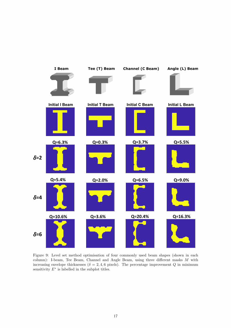
3.3 Beam shape optimisation

Now consider the cross-sections of four beam shapes commonly used in construction and engineer-

ing: an I-beam (or girder), T-beam (or Tee bar), C-beam (or Channel) and L-beam (or Angle

beam), shown in the top row of Figure 9. Shape optimisation is performed via the level set method

with three different masks M of increasing envelope thicknesses (δ = 2, 4, 6 pixels), where greater

14

i=0

Se

nsi

vity

ELL

Steel

Void

-20

-10

0

10

20

i) ψ j) ψ k) ψ l) ψ

ψ

o

n) Mean vi(x)

m

Me

an

vi(

x)

i=39 i=57 i=106

Figure 7: a-h) Demonstration of the shape optimisation algorithm using the level set method. Thefirst row shows component domain Ω, the second and third rows show the respective sensitivitymaps ELL and level set functions ψ. The initial shape is shown in panel (a) at algorithm iterationi = 0 with the corresponding sensitivity map ELL directly below (panel (e)) and the initial levelset function ψ0 in panel (i). Two intermediate component shapes are shown in panels (b) and (c),and the final optimised shape is shown in panel d. The minimum sensitivity E∗LL varying withiteration i during the optimisation is shown in plot (m). The mean of the velocity term vi(x) inEquation 14 is shown in plot (n) and the volume residual Vi(Ωi)− Vreq as a function of iteration iis shown in plot (o).

15

Void

Steel

M=0

M=1

∂Ω0

Figure 8: The example component considered in Figure 7 is reconsidered with a constrained designgiven by the mask M . a) The mask M used in Equation (17) for the constrained optimisation.The initial shape boundary ∂Ω0 is shown as a black dotted line. b) The optimised shape with amasking constraint. c) The evolution of the minimum sensitivity E∗LL as the algorithm iterates.d) The evolution of the volume fraction residual (Vi(Ω)− Vreq) as the algorithm iterates.

thickness allows larger perturbations from the initial component shapes; the domains are 100×100

pixels. The same optimisation parameters are used as those in Section 3.1, and the volume of the

initial component is preserved (Vreq = V0). The final shapes for the four initial components, and

for the different mask thicknesses are shown in Figure 9. The improvement in the minimum sensi-

tivity E∗ is quantified via Q, which is the percentage improvement in E∗ (Q = 100(E∗−E∗0 )/E∗0 ).

The values of Q are labelled in the titles of each subplot.

In all cases, there is an improvement in the minimum ultrasound sensitivity E∗, and generally

E∗ increases as the envelope width δ increases. In cases where only a small perturbation is admis-

sible (δ = 2), E∗ increases by as much as 6.3%. Where large perturbations are allowed (δ = 6),

E∗ increases by as much as 20.4%. Some similarities are noticeable for the optimal shapes for each

of the four component cross-sections. Both concave and convex corners become more rounded,

16

Q=6.3%

I Beam Tee (T) Beam Channel (C Beam) Angle (L) Beam

Q=0.3% Q=3.7% Q=5.5%

Q=5.4%

Q=10.6% Q=3.6% Q=20.4% Q=16.3%

Q=2.0% Q=6.5% Q=9.0%

=2

=4

=6

Figure 9: Level set method optimisation of four commonly used beam shapes (shown in eachcolumn): I-beam, Tee Beam, Channel and Angle Beam, using three different masks M withincreasing envelope thicknesses (δ = 2, 4, 6 pixels). The percentage improvement Q in minimumsensitivity E∗ is labelled in the subplot titles.

17

and indentations or protrusions are added to flat surfaces. These perturbations allow for a greater

range of incident angles for the ultrasonic transmission and receiver points, therefore improving ul-

trasonic sensitivity. These more complex designs are more challenging to build using conventional

manufacturing techniques, however additive manufacturing can easily manufacture such intricate

structures.

In these examples, only the ultrasonic sensitivity is optimised. In practice, the strength and

stiffness of the beam would also need to be considered, as any change in shape also alters the beam

mechanical properties. Such additional constraints can be factored into future optimisations.

3.4 TFM Imaging

While the use of ultrasonic sensitivity maps (for example ELL) is useful for the calculation of a

misfit function and the evolution of the level set function, the ability to image a defect, so that the

defect size and position can be better estimated, is fundamental to ultrasonic NDT. To quantify

the improvement in the imaging methods following the optimisation of a component’s shape, full

matrix capture (FMC) data is synthetically generated for a point defect (or point scatterer) located

at the point x∗ (the location of the minimum sensitivity E∗LL). That is

x∗ = argminx∈Ω

: ELL(x). (21)

The analytical expressions stated in Equations (3-6) give the recorded amplitude of a point

scatterer, and the arrival time of the recorded energy tsr is given by Equation (8). The reflectivity

P is calculated as

P (t; s, r,x∗) =SL(θs(x

∗))RL(θr(x∗))

[ds(x∗)dr(x∗)]1/2δ(t− tsr(x∗)) (22)

where δ is a unit impulse function. A 3 MHz Ricker wavelet (ξ(t)) is used for the source-time

function, and a synthetic recorded signal A (or A-scan) for source s, receiver r and scattering

point x∗ is then generated by convolving P (t) with the wavelet ξ(t), via

A(t; s, r,x∗) = P (t; s, r,x∗) ∗ ξ(t) +N(σ, t) (23)

where N(σ, t) is random Gaussian noise with standard deviation σ. A-scans for every source-

receiver combination are generated to produce a synthetic full matrix capture dataset.

TFM images were produced using the example initial square component shown in Figure 7a

and the optimised disk shape component shown in Figure 7d, (Fig. 10a and 10b, respectively),

where the scattering point x∗ is located in the centre of each component. Gaussian noise N

with a standard deviation σ = 0.1Pmax is used for both data sets, where Pmax is the maximum

18

a) Initial Shape TFM Image

2 4 6 8 10

X position (cm)

2

4

6

8

10

Y p

ositio

n (

cm

)

-30

-20

-10

0

b) Optimised Shape TFM Image

2 4 6 8 10

X position (cm)

2

4

6

8

10

Y p

ositio

n (

cm

)

-30

-20

-10

0

-0.05 0 0.05

X position (cm)

-14

-12

-10

-8

-6

-4

-2

0

TFM

Im

age T

ransect

(dB)

c) TFM Image Transects

Initial Shape

dB = 20log10(Iopt/Iopt)max

dB = 20log10(Iinit/Iinit)

dB = 20log10(Iopt/Iinit)max

Optimised Shape

Initial Shape Normalised to optimised maximum

True Defect Boundary

6 dB Threshold

True Defect Width

Initial Ω Estimate

Optimised Ω Estimate

3.0 mm

7.4 mm

3.9 mm

dB

dB

max

Figure 10: Comparison of total focusing method images of a point scatterer for a) the initial and b)the optimised shape (from the optimisation shown in Figure 7). c) Transects through the imagescompared with the true defect boundary width (dashed black line).

amplitude measured across both shapes Pmax = maxΩ |P |. An image is then generated using the

total focusing method via Equation (7), where the amplitudes in A are normalised to correct for

two-dimensional geometric spreading u(t; s, r,x∗) = A(t; s, r,x∗)/(VP t)2. To account for different

numbers of source-receiver pairs, which use different amounts of input energy, the intensities I are

normalised by the number of source-receiver pairs n2. Conventionally, TFM images are plotted in

decibels, normalised to the maximum amplitude in the respective image (dB = 20 log10(Imax/I)).

The resulting TFM images are shown in Figures 10a and b, and transects of these images shown

relative to the true locations of the defects x∗ are show in Figure 10c. To highlight the improvement

in the signal-to-noise ratio (SNR), the intensity values in the transect through the initial component

shape image Iinit are normalised with respect to the maximum intensity of the optimised image

(Ioptmax), and plotted as the yellow line in Fig. 10c. The image for the optimised shape has a

higher peak amplitude at the defect location and relative to the background material compared to

the image for the initial shape; there is an 8 dB improvement in the flaw image when using the

optimised design. When estimating the size of a defect, the -6 dB threshold is commonly used in

NDT [10]. Using this approach the estimated defect width in the initial and optimised components

is 7.4 mm and 3.9 mm, respectively, where the true defect width is 3.0 mm, so the percentage error

in sizing the defect is reduced from 100 × (7.3 − 3)/3 = 147% to 100 × (3.9 − 3)/3 = 30%. The

results for the optimised shape are therefore more robust to the addition of background noise and

more accurate in estimating the size of a defect.

19

4 Discussion

4.1 Limitations

This is the first presentation of a framework for shape optimisation that includes NDT consid-

erations. There are several limitations and potential extensions to the presented method. The

forward modelling approach uses an analytical model for the transmission and reception of laser

induced ultrasound [3, 29, 44]. This model is a first-order scattering approximation (waves are

reflected only once by a scatterer), and therefore does not consider any boundary reflections. Ray

tracing algorithms that account for reflections (e.g., Bai et al. [2]) or numerical simulation of wave

propagation [30, 33] could be implemented to include second order scattering better representing

the physics of wave propagation in practice. In addition to this, the optimisation only considers

the propagation of compressional (or longitudinal) waves (Equations (3) and (5)). A weighted

combination of compressional and transverse wave components [40] could be included in a future

implementation.

As the analytical model for the transmission and reception of laser induced ultrasound only

considers wave propagation in two dimensions, the shape optimisations presented here only consider

the perturbation of the two-dimensional cross-section of a three-dimensional component (rods

and beams) to enhance NDT capability. Current compliance-based level set shape and topology

optimisation algorithms are capable of designing intricate three-dimensional structures [21]. In

principle, our method can be applied similarly to more complex three-dimensional geometries

providing the analytical model that generates the ultrasonic wave propagation can account for

three dimensions.

Another simplification as presented here is the lack of topological variations during the level

set optimisation (i.e., there are no holes in Ω and no new holes are nucleated). Optimising for the

topology of a component is a major advantage of the level set method [1, 7], and is particularly

important in compliance-minimisation (stiffness maximisation) problems, where a stiff component

needs to be designed with a material volume constraint, so the nucleation of void regions is desir-

able. For ultrasonic NDT applications, the nucleation of voids introduces reflectors and barriers

to wave propagation, and therefore could cause difficulties for NDT. The extension of this method

to allow topological variations would be a natural extension to the current method; for example

allowing for joint optimisation for compliance and ultrasonic sensitivity.

4.2 Experimental Design and Joint Optimisation

In all the examples presented here, there is full coverage of the domain boundary by sources

and receivers, that is data is generated and recorded at every point on the boundary of a shape.

20

Realistically, such dense arrays of source and receiver locations are impractical, both due to the time

required to collect data as well as the memory requirements for such large datasets. Experimental

design describes a field of study that seeks to maximise the information in measured data by

optimising parameters, such as the number and distribution of sensors, while adhering to some

constraint on the cost of the experiment [9, 24]. The sensitivity of ultrasonic NDT (E) depends on

the distribution Γ of source s and receivers r, the material properties Ξ, and the spatial domain

of the component Ω, and as shown earlier E(x,Γ,Ξ,Ω). This paper has primarily focused on the

optimisation of the spatial domain Ω, however an optimisation of the source and receiver locations

Γ or material properties Ξ, or a joint optimisation for Ω,Ξ and Γ could be implemented.

To briefly illustrate this for an arbitrary component, an optimisation on the distribution of

sources and receivers Γ is performed for a randomly generated convex polygon with ten vertices

(Fig. 11), so that E∗LL is maximised via

Γ∗ = argmaxΓ∈∂Ω

: ELL(Γ,Ξ,Ω) (24)

where Ξ and Ω are held constant. As there are few degrees of freedom, a genetic algorithm can

be implemented (see appendix for algorithm information). An additional alternative approach is

an iterative grid search algorithm (IGSA, described in Algorithm 1). The IGSA iterates through

the desired number of source/receiver elements n1, performing a grid search for each element to

maximise E∗LL. This grid search is repeated for all elements a total of n2 times. Here the number

of elements n1 = 10, and the number of iterations n2 = 3 (here the total number of grid search

optimisations is n1 × n2 = 30).

Algorithm 1: Iterative grid search source and receiver optimisation algorithm. I is the it-eration and n2 is the maximum number of iterations. n1 is the number of sources/receiversand J is the index of each element (source/receiver location).

beginI = 1;J = 1;while I ≤ n2 do

while J ≤ n1 doΓ∗J = argmax

ΓJ∈∂Ω: E∗LL(Γ,Ξ,Ω);

I = I + 1;

endJ = J + 1;

end

end

The results are shown for the same component spatial domain Ω in Figure 11. The iterative

grid search method converges with a higher minimum sensitivity E∗LL and is less computationally

expensive. Such optimisations could be included in the current framework for shape optimisation,

21

a) Iterative Grid Search: ELL

*=6.09 b) Genetic Algorithm: E

LL

*=5.30

Figure 11: Comparison of the optimal distribution of source/receiver locations Γ∗ using (a) aniterative grid search method and (b) genetic algorithm. The source/receiver locations are shownas red circles.

such that the shape is optimised to maximise E∗, but where the minimum sensitivity E∗ is cal-

culated for the optimal distribution of a practical number of sources/receiver locations for each

shape considered.

5 Conclusion

A framework for including shape optimisation for ultrasonic non-destructive testing (NDT) in the

design of a component has been presented. Ultrasonic sensitivity maps are used to assess the

NDT suitability of a component using analytical expressions for the sensitivity of laser induced

ultrasound for detecting internal point scatterers. The optimal design of an I-beam cross-section,

obtained using a low number of degrees of freedom shape parameterisation and a genetic algorithm,

was implemented, and the ultrasonic sensitivity improved by a factor of two while remaining

within a design envelope. A level set method was then developed as a high number of degrees

of freedom (continuum) approach for shape optimisation for NDT on a range of commonly used

beam structures. Up to 20% improvement in ultrasonic sensitivity was achieved in the case where

design envelope and volume constraints were implemented. Flaw images computed using the

total focusing method on data arising from the inspection of the optimised shapes were shown

to be more robust to the presence of background noise, allowing for more accurate and precise

characterisation of internal defects; quantitatively there was an 8 dB improvement in SNR and a

five-fold improvement in the estimate of flaw size. Overall, these results show significant potential

for the use of a ‘Design for Testing’ framework to improve NDT capabilities and facilitate efficient

maintenance, life extension and remanufacturing processes, in turn minimizing production costs

and material waste.

22

6 Appendix: Genetic algorithm parameters

Table 2: The MATLAB (2019b) function ga (global optimization toolbox) parameters used forshape Ω and source/receiver geometry Γ optimisations.Genetic algorithm parameter Ω optimisation (Fig. 4) Γ optimisation (Fig. 11)Population size 50 200Generations 500 1000Cross-over fraction 0.8 0.8Elite count fraction 0.05 0.05

Mutation (MATLAB function)mutationgaussian:shrink=1,scale=1

mutationgaussian:shrink=1,scale=1

7 Acknowledgments

This work was funded by the Engineering and Physical Sciences Research Council (UK): grant

number EP/P005268/1.

8 Data Availability

The raw/processed data required to reproduce these findings cannot be shared at this time as the

data also forms part of an ongoing study. Individual MATLAB functions can be made available

by request to the authors.

References

[1] G. Allaire, F. Jouve, and A.-M. Toader. Structural optimization using sensitivity analysis anda level-set method. Journal of computational physics, 194(1):363–393, 2004.

[2] C. Bai, G. Huang, X. Li, B. Zhou, and S. Greenhalgh. Ray tracing of multiple transmit-ted/reflected/converted waves in 2-D/3-D layered anisotropic TTI media and application tocrosswell traveltime tomography. Geophysical Journal International, 195(2):1068–1087, 2013.

[3] J. R. Bernstein and J. B. Spicer. Line source representation for laser-generated ultrasound inaluminum. The Journal of the Acoustical Society of America, 107(3):1352–1357, 2000.

[4] J. P. Blasques and M. Stolpe. Multi-material topology optimization of laminated compositebeam cross sections. Composite Structures, 94(11):3278–3289, 2012.

[5] A. Blouin, D. Levesque, C. Neron, D. Drolet, and J.-P. Monchalin. Improved resolution andsignal-to-noise ratio in laser-ultrasonics by SAFT processing. Optics Express, 2(13):531–539,1998.

[6] P. Cawley. The rapid non-destructive inspection of large composite structures. Composites,25(5):351–357, 1994.

[7] V. J. Challis. A discrete level-set topology optimization code written in Matlab. Structuraland multidisciplinary optimization, 41(3):453–464, 2010.

[8] J. Chen, J. Xiao, D. Lisevych, and Z. Fan. Laser-induced full-matrix ultrasonic imagingof complex-shaped objects. IEEE transactions on ultrasonics, ferroelectrics, and frequencycontrol, 66(9):1514–1520, 2019.

23

[9] A. Curtis. Optimal design of focused experiments and surveys. Geophysical Journal Interna-tional, 139(1):205–215, 1999.

[10] J. Davies, F. Simonetti, M. Lowe, and P. Cawley. Review of synthetically focused guided waveimaging techniques with application to defect sizing. In AIP Conference Proceedings, volume820, pages 142–149. American Institute of Physics, 2006.

[11] P. Doyle. On epicentral waveforms for laser-generated ultrasound. Journal of Physics D:Applied Physics, 19(9):1613, 1986.

[12] M. Dubois, M. Militzer, A. Moreau, and J. F. Bussiere. A new technique for the quantitativereal-time monitoring of austenite grain growth in steel. Scripta materialia, 42(9), 2000.

[13] F. Gibou, R. Fedkiw, and S. Osher. A review of level-set methods and some recent applications.Journal of Computational Physics, 353:82–109, 2018.

[14] I. Gibson, D. W. Rosen, B. Stucker, et al. Additive manufacturing technologies, volume 17.Springer, 2014.

[15] G. Hatcher, W. Ijomah, and J. Windmill. Design for remanufacture: a literature review andfuture research needs. Journal of Cleaner Production, 19(17-18):2004–2014, 2011.

[16] C. Holmes, B. Drinkwater, and P. Wilcox. The post-processing of ultrasonic array data usingthe total focusing method. Insight-Non-Destructive Testing and Condition Monitoring, 46(11):677–680, 2004.

[17] C. Holmes, B. W. Drinkwater, and P. D. Wilcox. Post-processing of the full matrix of ultrasonictransmit–receive array data for non-destructive evaluation. NDT & E International, 38(8):701–711, 2005.

[18] C. Holmes, B. W. Drinkwater, and P. D. Wilcox. Advanced post-processing for scanned ultra-sonic arrays: Application to defect detection and classification in non-destructive evaluation.Ultrasonics, 48(6-7):636–642, 2008.

[19] W. L. Ijomah, C. A. McMahon, G. P. Hammond, and S. T. Newman. Development of designfor remanufacturing guidelines to support sustainable manufacturing. Robotics and Computer-Integrated Manufacturing, 23(6):712–719, 2007.

[20] Y. Javadi, C. N. MacLeod, S. G. Pierce, A. Gachagan, D. Lines, C. Mineo, J. Ding, S. Williams,M. Vasilev, E. Mohseni, et al. Ultrasonic phased array inspection of a Wire+ Arc AdditiveManufactured (WAAM) sample with intentionally embedded defects. Additive Manufacturing,29:100806, 2019.

[21] S. Kambampati, S. Townsend, and H. A. Kim. Aeroelastic level set topology optimization fora 3D wing. In 2018 AIAA/ASCE/AHS/ASC Structures, Structural Dynamics, and MaterialsConference, page 2151, 2018.

[22] Y. Y. Kim and T. S. Kim. Topology optimization of beam cross sections. International journalof solids and structures, 37(3):477–493, 2000.

[23] A. Koneru and K. Chakrabarty. Test and design-for-testability solutions for monolithic 3Dintegrated circuits. In Proceedings of the 2019 on Great Lakes Symposium on VLSI, pages457–462, 2019.

[24] N. Korta Martiartu, C. Boehm, V. Hapla, H. Maurer, I. J. Balic, and A. Fichtner. Optimalexperimental design for joint reflection-transmission ultrasound breast imaging: From ray-towave-based methods. The Journal of the Acoustical Society of America, 146(2):1252–1264,2019.

[25] J. Liang, W. Xu, C. Yue, K. Yu, H. Song, O. D. Crisalle, and B. Qu. Multimodal multiobjectiveoptimization with differential evolution. Swarm and evolutionary computation, 44:1028–1059,2019.

[26] D. Lines. Rapid inspection using integrated ultrasonic arrays. Insight: Non-DestructiveTesting and Condition Monitoring, 40(8):573–577, 1998.

24

[27] R. T. Lund. Remanufacturing: the experience of the USA and implications for the developingcountries. New York: World Bank Technical Papers, ISSN, pages 0253–7494, 1984.

[28] J. Luo, Z. Luo, L. Chen, L. Tong, and M. Y. Wang. A semi-implicit level set method forstructural shape and topology optimization. Journal of Computational Physics, 227(11):5561–5581, 2008.

[29] G. Miller and H. Pursey. The field and radiation impedance of mechanical radiators on the freesurface of a semi-infinite isotropic solid. Proceedings of the Royal Society of London. SeriesA. Mathematical and Physical Sciences, 223(1155):521–541, 1954.

[30] P. Moczo, J. O. Robertsson, and L. Eisner. The finite-difference time-domain method formodeling of seismic wave propagation. Advances in geophysics, 48:421–516, 2007.

[31] J.-P. Monchalin. Optical detection of ultrasound. IEEE Transactions on Ultrasonics Ferro-electrics and Frequency Control, 33:485–499, 1986.

[32] T. Morzadec, D. Marcha, and C. Duriez. Toward shape optimization of soft robots. In 20192nd IEEE International Conference on Soft Robotics (RoboSoft), pages 521–526. IEEE, 2019.

[33] F. Moser, L. J. Jacobs, and J. Qu. Modeling elastic wave propagation in waveguides with thefinite element method. NDT & E International, 32(4):225–234, 1999.

[34] M.-H. Noroy, D. Royer, and M. Fink. The laser-generated ultrasonic phased array: Analysisand experiments. The Journal of the Acoustical Society of America, 94(4):1934–1943, 1993.

[35] S. Osher, R. Fedkiw, and K. Piechor. Level set methods and dynamic implicit surfaces. Appl.Mech. Rev., 57(3):B15–B15, 2004.

[36] D. Pieris, T. Stratoudaki, Y. Javadi, P. Lukacs, S. Catchpole-Smith, P. D. Wilcox, A. Clare,and M. Clark. Laser induced phased arrays (LIPA) to detect nested features in additivelymanufactured components. Materials & Design, 187:108412, 2020.

[37] J. Plocher and A. Panesar. Review on design and structural optimisation in additive manu-facturing: Towards next-generation lightweight structures. Materials & Design, page 108164,2019.

[38] B. Raj, T. Jayakumar, and M. Thavasimuthu. Practical non-destructive testing. WoodheadPublishing, 2002.

[39] A. Riboni, L. Guglielmo, M. Orru, P. Braione, and G. Denaro. Design for testability of ERMTSapplications. In 2019 IEEE International Symposium on Software Reliability EngineeringWorkshops (ISSREW), pages 128–136. IEEE, 2019.

[40] L. Rose. Point-source representation for laser-generated ultrasound. The Journal of theAcoustical Society of America, 75(3):723–732, 1984.

[41] L. W. Schmerr. Fundamentals of ultrasonic nondestructive evaluation. Springer, 2016.

[42] J. A. Sethian. Level set methods and fast marching methods: evolving interfaces in compu-tational geometry, fluid mechanics, computer vision, and materials science, volume 3. Cam-bridge university press, 1999.

[43] W. Song and A. Keane. A study of shape parameterisation methods for airfoil optimisation. In10th AIAA/ISSMO Multidisciplinary analysis and optimization conference, page 4482, 2004.

[44] T. Stratoudaki, M. Clark, and P. D. Wilcox. Laser induced ultrasonic phased array usingfull matrix capture data acquisition and total focusing method. Optics express, 24(19):21921–21938, 2016.

[45] T. Stratoudaki, Y. Javadi, W. Kerr, P. D. Wilcox, D. Pieris, and M. Clark. Laser inducedphased arrays for remote ultrasonic imaging of additive manufactured components. In 57thAnnual Conference of the British Institute of Non-Destructive Testing, NDT 2018, pages174–182, 2018.

25

[46] K. M. Tant, E. Galetti, A. Mulholland, A. Curtis, and A. Gachagan. A transdimensionalbayesian approach to ultrasonic travel-time tomography for non-destructive testing. InverseProblems, 34(9):095002, 2018.

[47] K. M. Tant, A. J. Mulholland, A. Curtis, and W. L. Ijomah. Design-for-testing for improvedremanufacturability. Journal of Remanufacturing, 9(1):61–72, 2019.

[48] K. M. M. Tant, E. Galetti, A. Mulholland, A. Curtis, and A. Gachagan. Effective grain orien-tation mapping of complex and locally anisotropic media for improved imaging in ultrasonicnon-destructive testing. Inverse Problems in Science and Engineering, pages 1–25, 2020.

[49] L.-S. Wang, J. S. Steckenrider, and J. D. Achenbach. A fiber-based laser ultrasonic systemfor remote inspection of limited access components. In Review of Progress in QuantitativeNondestructive Evaluation, pages 507–514. Springer, 1997.

[50] M. Y. Wang, X. Wang, and D. Guo. A level set method for structural topology optimization.Computer methods in applied mechanics and engineering, 192(1-2):227–246, 2003.

[51] R. M. White. Generation of elastic waves by transient surface heating. Journal of AppliedPhysics, 34(12):3559–3567, 1963.

[52] D. Whitley. A genetic algorithm tutorial. Statistics and computing, 4(2):65–85, 1994.

[53] P. D. Wilcox. Ultrasonic arrays in NDE: Beyond the B-scan. In AIP Conference Proceedings,volume 1511, pages 33–50. American Institute of Physics, 2013.

[54] K. R. Yawn, M. A. Osterkamp, D. Kaiser, and C. Barina. Improved laser ultrasonic systemsfor industry. In AIP Conference Proceedings, volume 1581, pages 397–404. American Instituteof Physics, 2014.

26