complex systems methods --- 9. critical phenomena: the ... · h¯0 = rh¯ the renormalization group...
TRANSCRIPT

Complex Systems Methods — 9. Critical Phenomena:The Renormalization Group
Eckehard Olbrich
[email protected]://personal-homepages.mis.mpg.de/olbrich/complex systems.html
Potsdam WS 2007/08
Olbrich (Leipzig) 11.01.2007 1 / 21

Overview
1 The general schemeThe renormalization group transformationFlows in parameter spaceUniversality and CrossoverScaling and critical exponents
2 Implementation of the renormalization groupThe one-dimensional Ising modelHigher dimensions — the 2D-Ising model
Olbrich (Leipzig) 11.01.2007 2 / 21

Scaling, Renormalization and Universality
Start with some model M(xxx ,ppp) defined on some scale ε withparameters ppp.
Now define new observable xxx ′ by coarse graining, e.g. integrating theold ones over a certain range. Then rescale the new variables, suchthat the model for the new variables is in the same space as theoriginal one, but usually with different parameters ppp′.
Thus we get a map (or flow) ppp 7→ ppp′ in the parameter space, with asemigroup property, the renormalization group (RG).
Self-similar system state ⇒ fixed point of the transformation ⇒critical states are unstable fixed points of the RG transformation.
Stable manifolds of these fixed points represent different modelsshowing the same critical behavior ⇒ universality
Critical exponents can be derived from the fixed point properties ⇒they are equal in one universality class
Olbrich (Leipzig) 11.01.2007 3 / 21

What can be explained by the renormalization group?
Continuous phase transitions fall into universality classescharacterized by a given value of the critical exponents.
For a given universality class there is an upper critical dimensionabove which the exponents take on mean-field values.
Relations between exponents, which follows as inequalities fromthermodynamics, hold as equalities.
Critical exponents take the same value as the transition temperatureis approached from above or below.
Olbrich (Leipzig) 11.01.2007 4 / 21

The renormalization group transformation
Literature: J. M. Yeomans, Statistical Mechanics of Phase Transitions,Oxford University Press, 1992.
Starting point: reduced Hamiltonian H̄ ≡ H/kT
Renormalization group operator RRR transforms the reducedHamiltonian in a new one
H̄′ = RRRH̄
Olbrich (Leipzig) 11.01.2007 5 / 21

The renormalization group transformation
Starting point: reduced Hamiltonian H̄ ≡ H/kT
Renormalization group operator RRR transforms the reducedHamiltonian in a new one
H̄′ = RRRH̄
The renormalization group operator decreases the number of degreesof freedom from N to N ′ — either in real space by removing orgrouping spins, or in reciprocal space, by integrating out largewavevectors, i.e. removing small wavelength. The scale factor of thetransformation, b, is defined by
bd = N/N ′
with d denoting the dimensionality of the system.
Olbrich (Leipzig) 11.01.2007 5 / 21

The renormalization group transformation
Starting point: reduced Hamiltonian H̄ ≡ H/kT
Renormalization group operator RRR transforms the reducedHamiltonian in a new one
H̄′ = RRRH̄
Scale factorbd = N/N ′
The essential condition to be satisfied by any renormalization grouptransformation is that the partition function must not change:
ZN′(H̄′) = ZN(H̄) .
Olbrich (Leipzig) 11.01.2007 5 / 21

The renormalization group transformation
Starting point: reduced Hamiltonian H̄ ≡ H/kT
Renormalization group operator RRR transforms the reducedHamiltonian in a new one
H̄′ = RRRH̄
Scale factorbd = N/N ′
Partition function must not change
ZN′(H̄′) = ZN(H̄) .
Reduced free energy per spin (unit volume) f̄ = f /kT transforms as
f̄ (H̄′) = bd f̄ (H̄)
Olbrich (Leipzig) 11.01.2007 5 / 21

Flows in parameter space
General reduced Hamiltonian
H̄ =∑α
µµµ.∫∫∫
with functions (usually products) of system variables ∫∫∫ andconjugated fields µµµ.
E.g. in the case of the Ising model
H̄ = −∑
i
C − h∑
i
si − K∑〈ij〉
si sj − J∑〈ijkl〉
si sjsksl − . . .
we have ∫∫∫ = (1, si , si sj , si sjsksl , . . .),µµµ = (C , h,K , J, . . .).
Fields µµµ parametrize the reduced Hamiltonian. Application of therenormalization operator moves the system through parameter space
µ′µ′µ′ = RRRµµµ .
Olbrich (Leipzig) 11.01.2007 6 / 21

Fixed points of the renormalization operator
µ′µ′µ′ = RRRµµµ µ∗µ∗µ∗ := µµµ with µ′µ′µ′ = µµµ .
Linearization around the fixed point
µµµ = µ∗µ∗µ∗ + δµµµ
µ′µ′µ′ = µ∗µ∗µ∗ + δµ′µ′µ′
leads toδµ′µ′µ′ = AAA(µ∗µ∗µ∗)δµµµ
with AAA being the linearization of RRR at µ∗µ∗µ∗. Being λi and vvv i the eigenvaluesand eigenvectors of AAA, respectively, we get for two successivetransformations with scaling factors b1 and b2
λi (b1)λi (b2) = λi (b1b2)
and thereforeλi (b) = byi .
Olbrich (Leipzig) 11.01.2007 7 / 21

Renormalization near the fixed point
Expand the deviation from the fixed point in terms of the eigenvectors ofAAA, vvv i
µµµ = µ∗µ∗µ∗ +∑
i
givvv i .
The coefficients gi are termed the linear scaling fields. Applying RRR leads to
µ′µ′µ′ = µ∗µ∗µ∗ +∑
i
byi givvv i or
g ′i = byi gi respectively.
yi > 0: unstable directions, relevant scaling fields ⇒ controlparameters
yi = 0: marginal stable directions
yi < 0: stable directions, irrelevant scaling fields ⇒ critical surface,universality
Olbrich (Leipzig) 11.01.2007 8 / 21

Universality
Universality: Under renormalization (scale change) the irrelevant scalingfields will decrease and the system will flow toward the fixed point, whilethe relevant will increase, driving it away from the critical surface. As longas the relevant fields are initially small enough the trajectory will comeclose to the fixed point. Therefore its critical behavior will be determinedby the linearized transformation at the fixed point and will be independentof the original values of the irrelevant scaling fields.
Olbrich (Leipzig) 11.01.2007 9 / 21

Crossover
Crossover: If there is more than one fixed point embedded in the criticalsurface crossover effects may occur. For example in a magnetic systemwith weak spin anisotropy as the temperature approaches Tc , the systemexhibits Heisenberg critical behavior (A), but very close to Tc the criticalexponents change to those corresponding to an Ising system (B).
Olbrich (Leipzig) 11.01.2007 10 / 21

Scaling and critical exponents
The singular part of the rescaled free energy per spin f̄ = f /KT wastransformed as
f̄ (µµµ) = b−d f̄ (µµµ′)
Near the fixed point we have
f̄ (g1, g2, g3, . . .) ∝ b−d f̄ (by1g1, by2g2, b
y2g2, . . .)
thus f̄ is a generalized homogeneous function.If there are two relevant scaling field (as in the example of the Isingmodel) we set g1 = t = (T − Tc)/T and g2 = h = H/kT . Thus
f̄ (t, h, g3, . . .) ∝ b−d f̄ (by1t, by2h, by3g3, . . .)
as t, h, g3 → 0.
Olbrich (Leipzig) 11.01.2007 11 / 21

Scaling and critical exponents
Free energy:f̄ (t, h, 0, . . .) ∝ b−d f̄ (by1t, by2h, 0, . . .)
Specific heat:
C ∝(
∂2f̄
∂t2
)h=0
≡ f̄tt(h = 0) ∝ |t|−α
leads tof̄tt(h = 0) ∝ b−d+2y1 f̄tt(b
y1 t, 0) .
Choosing by1 |t| = 1 gives then
f̄tt(h = 0) ∝ |t|(d−2y1)/y1 f̄tt(±1, 0)
and thereforeα = 2− d/y1
Olbrich (Leipzig) 11.01.2007 12 / 21

Scaling and critical exponents
Specific heat: α = 2− d/y1
Magnetization as function of the temperature: β = (d − y2)/y1
Susceptibility: γ = (2− y2 − d)/y1
Magnetization as function of the magnetic field: δ = y2/(d − y2)
Equations:
α + 2β + γ = 2 corresponds to Rushbrooke inequality
γ = β(δ − 1) corresponds to Widom inequality
2-d Ising Model: α = 0, β = 1/8, γ = 7/4, δ = 15.
Olbrich (Leipzig) 11.01.2007 13 / 21
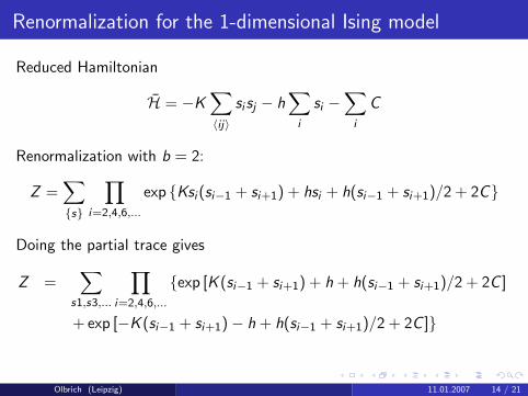
Renormalization for the 1-dimensional Ising model
Reduced Hamiltonian
H̄ = −K∑〈ij〉
si sj − h∑
i
si −∑
i
C
Renormalization with b = 2:
Z =∑{s}
∏i=2,4,6,...
exp {Ksi (si−1 + si+1) + hsi + h(si−1 + si+1)/2 + 2C}
Doing the partial trace gives
Z =∑
s1,s3,...
∏i=2,4,6,...
{exp [K (si−1 + si+1) + h + h(si−1 + si+1)/2 + 2C ]
+ exp [−K (si−1 + si+1)− h + h(si−1 + si+1)/2 + 2C ]}
Olbrich (Leipzig) 11.01.2007 14 / 21

Renormalization for the 1-dimensional Ising model
Reduced Hamiltonian
H̄ = −K∑〈ij〉
si sj − h∑
i
si −∑
i
C
Renormalization with b = 2:
Z =∑{s}
∏i=2,4,6,...
exp {Ksi (si−1 + si+1) + hsi + h(si−1 + si+1)/2 + 2C}
Relabeling the spins:
Z =∑{s}
∏i
{exp
[(K +
h
2)(si + si+1) + h + 2C
]
+exp
[−(K − h
2)(si + si+1) + h + 2C
]}
Olbrich (Leipzig) 11.01.2007 14 / 21

Renormalization for the 1-dimensional Ising model
Reduced Hamiltonian
H̄ = −K∑〈ij〉
si sj − h∑
i
si −∑
i
C
Renormalization with b = 2:
Z =∑{s}
∏i
{exp
[(K +
h
2)(si + si+1) + h + 2C
]
+exp
[−(K − h
2)(si + si+1) + h + 2C
]}=
∑{s}
∏i
exp(K ′si si+1 + h′si + C ′) .
Olbrich (Leipzig) 11.01.2007 14 / 21
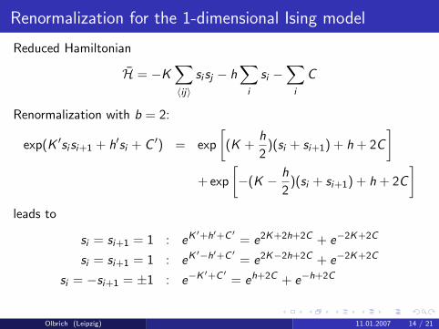
Renormalization for the 1-dimensional Ising model
Reduced Hamiltonian
H̄ = −K∑〈ij〉
si sj − h∑
i
si −∑
i
C
Renormalization with b = 2:
exp(K ′si si+1 + h′si + C ′) = exp
[(K +
h
2)(si + si+1) + h + 2C
]+exp
[−(K − h
2)(si + si+1) + h + 2C
]leads to
si = si+1 = 1 : eK ′+h′+C ′= e2K+2h+2C + e−2K+2C
si = si+1 = 1 : eK ′−h′+C ′= e2K−2h+2C + e−2K+2C
si = −si+1 = ±1 : e−K ′+C ′= eh+2C + e−h+2C
Olbrich (Leipzig) 11.01.2007 14 / 21

Renormalization equations
si = si+1 = 1 : eK ′+h′+C ′= e2K+2h+2C + e−2K+2C
si = si+1 = 1 : eK ′−h′+C ′= e2K−2h+2C + e−2K+2C
si = −si+1 = ±1 : e−K ′+C ′= eh+2C + e−h+2C
leads to
e2h′= (e2h + e−4K )(e−2h + e−4K )−1
e4C ′= e8Ce4K (e2h + e−4K )(e−2h + e−4K )e2h(1 + e−2h)2
e4K ′= e4K (e2h + e−4K )(e−2h + e−4K )e−2h(1 + e−2h)−2
Olbrich (Leipzig) 11.01.2007 15 / 21

Renormalization equations
e2h′= (e2h + e−4K )(e−2h + e−4K )−1
e4C ′= e8Ce4K (e2h + e−4K )(e−2h + e−4K )e2h(1 + e−2h)2
e4K ′= e4K (e2h + e−4K )(e−2h + e−4K )e−2h(1 + e−2h)−2
and with x = e−4K ,y = e−2h and ω = e−4C
ω′ =ω2xy2
(1 + xy)(x + y)(1 + y)2
x ′ =x(1 + y)2
(1 + xy)(x + y)
y ′ =y(x + y)
1 + yx.
Olbrich (Leipzig) 11.01.2007 16 / 21

Fixed points
x ′ =x(1 + y)2
(1 + xy)(x + y)
y ′ =y(x + y)
1 + yx
Fixed points for ferromagnetic couplingK > 0.High temperature: x = 1 0 ≤ y ≤1 — infinite temperature, paramagneticfixed point, attractingLow temperature and infinite field: x = 0and y = 0 — fully aligned configurationFerromagnetic fixed point: x = 0 andy = 1
Olbrich (Leipzig) 11.01.2007 17 / 21

Scaling at the ferromagnetic fixed point
Linearizing the low equations around the fixed point (x , y) = (0, 1) gives
δx ′ = 4δx δy ′ = 2δy .
Hence the eigenvalues of the linearized transformation are
λ1 = 4 λ2 = 2
and because of the scale factor b = 2 we have
y1 =lnλ1
ln b= 2 y2 = 1 .
Problem: Tc = 0, thus t = (T − Tc)/Tc = ∞ and the usual criticalexponents are not defined.
Olbrich (Leipzig) 11.01.2007 18 / 21

Higher dimensions — the 2D-Ising model
If s denoting the remaining and t the spins that are integrated out one hasto consider terms such as
expKs00(t01 + t0−1 + t10 + t−10)
Taking the trace over s00 gives
2 cosh K (t01 + t0−1 + t10 + t−10)
which can be rewritten as
exp {a(K ) + b(K )(t−10t01 + t10t01 + t10t0−1
+t−10t0−1 + t−10t10 + t0−1t01) + c(K )t−10t01t10t0−1}
Olbrich (Leipzig) 11.01.2007 19 / 21

Higher dimensions — the 2D-Ising model
If s denoting the remaining and t the spins that are integrated out one hasto consider terms such as
expKs00(t01 + t0−1 + t10 + t−10)
Taking the trace over s00 gives
exp {a(K ) + b(K )(t−10t01 + t10t01 + t10t0−1
+t−10t0−1 + t−10t10 + t0−1t01) + c(K )t−10t01t10t0−1}
a(K ) = ln 2 + (ln cosh 4K + 4 ln cosh 2K )/8
b(K ) = (ln cosh 4K )/8
c(K ) = (ln cosh 4K − 4 ln cosh 2K )/8
Olbrich (Leipzig) 11.01.2007 19 / 21

Higher dimensions — the 2D-Ising model
If s denoting the remaining and t the spins that are integrated out one hasto consider terms such as
expKs00(t01 + t0−1 + t10 + t−10)
Taking the trace over s00 gives
exp {a(K ) + b(K )(t−10t01 + t10t01 + t10t0−1
+t−10t0−1 + t−10t10 + t0−1t01) + c(K )t−10t01t10t0−1}
H̄′ = 2b(K )∑〈ij〉
ti tj + b(K )∑[ij]
ti tj + c(K )∑sq
ti tj tktl
with [ij ] denoting second neighbors and sq neighbors around a elementarysquare on the renormlized lattice.
Olbrich (Leipzig) 11.01.2007 19 / 21

Higher Dimensions
Starting from next nearest interaction the renormalization proceduregenerates new (longer range) interaction terms.
In the case of the 2D-Ising model already the second step of the realspace renormalization cannot be made straight forward.
in general no exact derivation of the renormalization equationspossible.
Approximations are necessary, e.g. Kadanoffs block spin procedure
ε-expansion with respect to the dimension d = 4− ε in cases where 4is the upper critical dimension is carried out in k-space
Numerical methods: Monte-Carlo renormalization group
Olbrich (Leipzig) 11.01.2007 20 / 21

Outlook: Self-organized criticality (SOC)
Up to now we only considered the partition function, i.e. no dynamics.
Dimension of the unstable manifold of the critical fixed point of therenormalization flow — number of control parameters that have to beadjusted to reach the critical state
SOC: Dynamical system which involves the control parameters anddrives them to the critical point
Olbrich (Leipzig) 11.01.2007 21 / 21