complex adaptive dynamical systems, a primer · 1 complex adaptive dynamical systems, a primer1...
TRANSCRIPT

1
Complex Adaptive Dynamical
Systems, a Primer1
2008/10
Claudius GrosInstitute for Theoretical Physics
Goethe University Frankfurt
1Springer 2008, second edition 2010; including the solution section.
arX
iv:0
807.
4838
v3 [
nlin
.AO
] 2
5 Se
p 20
12

2

Contents
1 Graph Theory and Small-World Networks 11.1 Graph Theory and Real-World Networks . . . . . . . . . . . . . . . . 1
1.1.1 The Small-World Effect . . . . . . . . . . . . . . . . . . . . 11.1.2 Basic Graph-Theoretical Concepts . . . . . . . . . . . . . . . 31.1.3 Properties of Random Graphs . . . . . . . . . . . . . . . . . 8
1.2 Generalized Random Graphs . . . . . . . . . . . . . . . . . . . . . . 131.2.1 Graphs with Arbitrary Degree Distributions . . . . . . . . . . 131.2.2 Probability Generating Function Formalism . . . . . . . . . . 171.2.3 Distribution of Component Sizes . . . . . . . . . . . . . . . . 20
1.3 Robustness of Random Networks . . . . . . . . . . . . . . . . . . . . 221.4 Small-World Models . . . . . . . . . . . . . . . . . . . . . . . . . . 261.5 Scale-Free Graphs . . . . . . . . . . . . . . . . . . . . . . . . . . . . 28Exercises . . . . . . . . . . . . . . . . . . . . . . . . . . . . . . . . . . . 32Further Reading . . . . . . . . . . . . . . . . . . . . . . . . . . . . . . . . 33
2 Chaos, Bifurcations and Diffusion 372.1 Basic Concepts of Dynamical Systems Theory . . . . . . . . . . . . . 372.2 The Logistic Map and Deterministic Chaos . . . . . . . . . . . . . . 422.3 Dissipation and Adaption . . . . . . . . . . . . . . . . . . . . . . . . 47
2.3.1 Dissipative Systems and Strange Attractors . . . . . . . . . . 482.3.2 Adaptive Systems . . . . . . . . . . . . . . . . . . . . . . . . 52
2.4 Diffusion and Transport . . . . . . . . . . . . . . . . . . . . . . . . . 562.4.1 Random Walks, Diffusion and Levy Flights . . . . . . . . . . 562.4.2 The Langevin Equation and Diffusion . . . . . . . . . . . . . 60
2.5 Noise-Controlled Dynamics . . . . . . . . . . . . . . . . . . . . . . 612.5.1 Stochastic Escape . . . . . . . . . . . . . . . . . . . . . . . . 622.5.2 Stochastic Resonance . . . . . . . . . . . . . . . . . . . . . . 65
2.6 Dynamical Systems with Time Delays . . . . . . . . . . . . . . . . . 67Exercises . . . . . . . . . . . . . . . . . . . . . . . . . . . . . . . . . . . 71Further Reading . . . . . . . . . . . . . . . . . . . . . . . . . . . . . . . . 72
i

ii CONTENTS
3 Complexity and Information Theory 753.1 Probability Distribution Functions . . . . . . . . . . . . . . . . . . . 75
3.1.1 The Law of Large Numbers . . . . . . . . . . . . . . . . . . 783.1.2 Time Series Characterization . . . . . . . . . . . . . . . . . . 80
3.2 Entropy and Information . . . . . . . . . . . . . . . . . . . . . . . . 823.2.1 Information Content of a Real-World Time Series . . . . . . . 883.2.2 Mutual Information . . . . . . . . . . . . . . . . . . . . . . . 89
3.3 Complexity Measures . . . . . . . . . . . . . . . . . . . . . . . . . . 933.3.1 Complexity and Predictability . . . . . . . . . . . . . . . . . 953.3.2 Algorithmic and Generative Complexity . . . . . . . . . . . . 97
Exercises . . . . . . . . . . . . . . . . . . . . . . . . . . . . . . . . . . . 99Further Reading . . . . . . . . . . . . . . . . . . . . . . . . . . . . . . . . 100
4 Random Boolean Networks 1034.1 Introduction . . . . . . . . . . . . . . . . . . . . . . . . . . . . . . . 1034.2 Random Variables and Networks . . . . . . . . . . . . . . . . . . . . 105
4.2.1 Boolean Variables and Graph Topologies . . . . . . . . . . . 1054.2.2 Coupling Functions . . . . . . . . . . . . . . . . . . . . . . . 1074.2.3 Dynamics . . . . . . . . . . . . . . . . . . . . . . . . . . . . 108
4.3 The Dynamics of Boolean Networks . . . . . . . . . . . . . . . . . . 1094.3.1 The Flow of Information Through the Network . . . . . . . . 1104.3.2 The Mean-Field Phase Diagram . . . . . . . . . . . . . . . . 1124.3.3 The Bifurcation Phase Diagram . . . . . . . . . . . . . . . . 1134.3.4 Scale-Free Boolean Networks . . . . . . . . . . . . . . . . . 117
4.4 Cycles and Attractors . . . . . . . . . . . . . . . . . . . . . . . . . . 1194.4.1 Quenched Boolean Dynamics . . . . . . . . . . . . . . . . . 1194.4.2 The K = 1 Kauffman Network . . . . . . . . . . . . . . . . . 1224.4.3 The K = 2 Kauffman Network . . . . . . . . . . . . . . . . . 1234.4.4 The K = N Kauffman Network . . . . . . . . . . . . . . . . . 124
4.5 Applications . . . . . . . . . . . . . . . . . . . . . . . . . . . . . . . 1264.5.1 Living at the Edge of Chaos . . . . . . . . . . . . . . . . . . 1264.5.2 The Yeast Cell Cycle . . . . . . . . . . . . . . . . . . . . . . 1284.5.3 Application to Neural Networks . . . . . . . . . . . . . . . . 130
Exercises . . . . . . . . . . . . . . . . . . . . . . . . . . . . . . . . . . . 131Further Reading . . . . . . . . . . . . . . . . . . . . . . . . . . . . . . . . 132
5 Cellular Automata and Self-Organized Criticality 1375.1 The Landau Theory of Phase Transitions . . . . . . . . . . . . . . . . 1375.2 Criticality in Dynamical Systems . . . . . . . . . . . . . . . . . . . . 142
5.2.1 1/f Noise . . . . . . . . . . . . . . . . . . . . . . . . . . . . 1455.3 Cellular Automata . . . . . . . . . . . . . . . . . . . . . . . . . . . . 146
5.3.1 Conway’s Game of Life . . . . . . . . . . . . . . . . . . . . 1475.3.2 The Forest Fire Model . . . . . . . . . . . . . . . . . . . . . 148
5.4 The Sandpile Model and Self-Organized Criticality . . . . . . . . . . 1505.5 Random Branching Theory . . . . . . . . . . . . . . . . . . . . . . . 152
5.5.1 Branching Theory of Self-Organized Criticality . . . . . . . . 152

CONTENTS iii
5.5.2 Galton-Watson Processes . . . . . . . . . . . . . . . . . . . . 1575.6 Application to Long-Term Evolution . . . . . . . . . . . . . . . . . . 158Exercises . . . . . . . . . . . . . . . . . . . . . . . . . . . . . . . . . . . 165Further Reading . . . . . . . . . . . . . . . . . . . . . . . . . . . . . . . . 166
6 Darwinian Evolution, Hypercycles and Game Theory 1696.1 Introduction . . . . . . . . . . . . . . . . . . . . . . . . . . . . . . . 1696.2 Mutations and Fitness in a Static Environment . . . . . . . . . . . . . 1716.3 Deterministic Evolution . . . . . . . . . . . . . . . . . . . . . . . . . 174
6.3.1 Evolution Equations . . . . . . . . . . . . . . . . . . . . . . 1756.3.2 Beanbag Genetics – Evolutions Without Epistasis . . . . . . . 1786.3.3 Epistatic Interactions and the Error Catastrophe . . . . . . . . 180
6.4 Finite Populations and Stochastic Escape . . . . . . . . . . . . . . . . 1836.4.1 Strong Selective Pressure and Adaptive Climbing . . . . . . . 1846.4.2 Adaptive Climbing Versus Stochastic Escape . . . . . . . . . 187
6.5 Prebiotic Evolution . . . . . . . . . . . . . . . . . . . . . . . . . . . 1886.5.1 Quasispecies Theory . . . . . . . . . . . . . . . . . . . . . . 1886.5.2 Hypercycles and Autocatalytic Networks . . . . . . . . . . . 190
6.6 Coevolution and Game Theory . . . . . . . . . . . . . . . . . . . . . 193Exercises . . . . . . . . . . . . . . . . . . . . . . . . . . . . . . . . . . . 198Further Reading . . . . . . . . . . . . . . . . . . . . . . . . . . . . . . . . 200
7 Synchronization Phenomena 2037.1 Frequency Locking . . . . . . . . . . . . . . . . . . . . . . . . . . . 2037.2 Synchronization of Coupled Oscillators . . . . . . . . . . . . . . . . 2047.3 Synchronization with Time Delays . . . . . . . . . . . . . . . . . . . 2107.4 Synchronization via Aggregate Averaging . . . . . . . . . . . . . . . 2127.5 Synchronization via Causal Signaling . . . . . . . . . . . . . . . . . 2157.6 Synchronization and Object Recognition in Neural Networks . . . . . 2197.7 Synchronization Phenomena in Epidemics . . . . . . . . . . . . . . . 222Exercises . . . . . . . . . . . . . . . . . . . . . . . . . . . . . . . . . . . 225Further Reading . . . . . . . . . . . . . . . . . . . . . . . . . . . . . . . . 227
8 Elements of Cognitive Systems Theory 2298.1 Introduction . . . . . . . . . . . . . . . . . . . . . . . . . . . . . . . 2298.2 Foundations of Cognitive Systems Theory . . . . . . . . . . . . . . . 231
8.2.1 Basic Requirements for the Dynamics . . . . . . . . . . . . . 2318.2.2 Cognitive Information Processing Versus Diffusive Control . . 2358.2.3 Basic Layout Principles . . . . . . . . . . . . . . . . . . . . 2368.2.4 Learning and Memory Representations . . . . . . . . . . . . 238
8.3 Motivation, Benchmarks and Diffusive Emotional Control . . . . . . 2428.3.1 Cognitive Tasks . . . . . . . . . . . . . . . . . . . . . . . . . 2438.3.2 Internal Benchmarks . . . . . . . . . . . . . . . . . . . . . . 243
8.4 Competitive Dynamics and Winning Coalitions . . . . . . . . . . . . 2478.4.1 General Considerations . . . . . . . . . . . . . . . . . . . . . 2488.4.2 Associative Thought Processes . . . . . . . . . . . . . . . . . 2528.4.3 Autonomous Online Learning . . . . . . . . . . . . . . . . . 256

iv CONTENTS
8.5 Environmental Model Building . . . . . . . . . . . . . . . . . . . . . 2588.5.1 The Elman Simple Recurrent Network . . . . . . . . . . . . . 2588.5.2 Universal Prediction Tasks . . . . . . . . . . . . . . . . . . . 262
Exercises . . . . . . . . . . . . . . . . . . . . . . . . . . . . . . . . . . . 265Further Reading . . . . . . . . . . . . . . . . . . . . . . . . . . . . . . . . 265

Chapter 1
Graph Theory and Small-WorldNetworks
Dynamical networks constitute a very wide class of complex and adaptive systems.Examples range from ecological prey–predator networks to the gene expression andprotein networks constituting the basis of all living creatures as we know it. The brainis probably the most complex of all adaptive dynamical systems and is at the basis ofour own identity, in the form of a sophisticated neural network. On a social level weinteract through social networks, to give a further example – networks are ubiquitousthrough the domain of all living creatures.
A good understanding of network theory is therefore of basic importance for com-plex system theory. In this chapter we will discuss the most important concepts ofgraph1 theory and basic realizations of possible network organizations.
1.1 Graph Theory and Real-World Networks
1.1.1 The Small-World EffectSix or more billion humans live on earth today and it might seem that the world is a bigplace. But, as an Italian proverb says,
“Tutto il mondo e paese” – “The world is a village”.
The network of who knows whom – the network of acquaintances – is indeed quitedensely webbed. Modern scientific investigations mirror this century-old proverb.Social Networks Stanley Milgram performed a by now famous experiment in the1960s. He distributed a number of letters addressed to a stockbroker in Boston to arandom selection of people in Nebraska. The task was to send these letters to theaddressee (the stockbroker) via mail to an acquaintance of the respective sender. Inother words, the letters were to be sent via a social network.
1Mathematicians generally prefer the somewhat more abstract term “graph” instead of “network”.
1
2 CHAPTER 1. GRAPH THEORY AND SMALL-WORLD NETWORKS
B
D
A
C
E
F
G
H
I
J
K
A B C D E F G H I J K
1 2 3 4
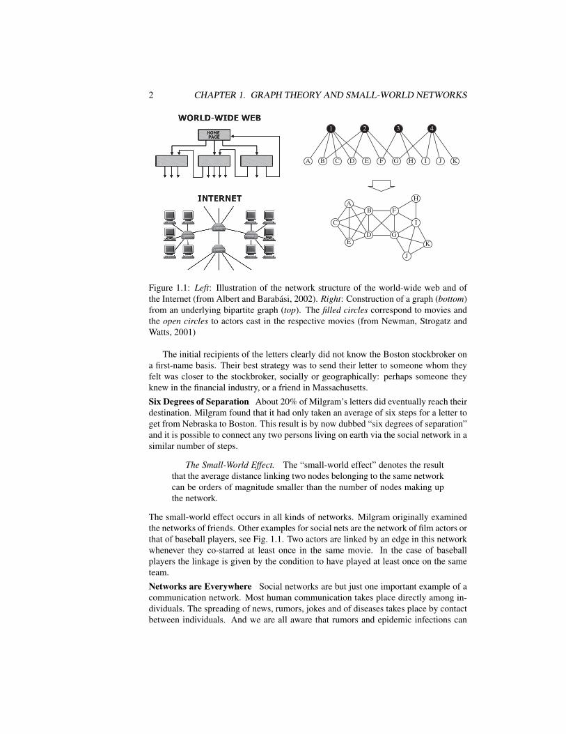
Figure 1.1: Left: Illustration of the network structure of the world-wide web and ofthe Internet (from Albert and Barabasi, 2002). Right: Construction of a graph (bottom)from an underlying bipartite graph (top). The filled circles correspond to movies andthe open circles to actors cast in the respective movies (from Newman, Strogatz andWatts, 2001)
The initial recipients of the letters clearly did not know the Boston stockbroker ona first-name basis. Their best strategy was to send their letter to someone whom theyfelt was closer to the stockbroker, socially or geographically: perhaps someone theyknew in the financial industry, or a friend in Massachusetts.
Six Degrees of Separation About 20% of Milgram’s letters did eventually reach theirdestination. Milgram found that it had only taken an average of six steps for a letter toget from Nebraska to Boston. This result is by now dubbed “six degrees of separation”and it is possible to connect any two persons living on earth via the social network in asimilar number of steps.
The Small-World Effect. The “small-world effect” denotes the resultthat the average distance linking two nodes belonging to the same networkcan be orders of magnitude smaller than the number of nodes making upthe network.
The small-world effect occurs in all kinds of networks. Milgram originally examinedthe networks of friends. Other examples for social nets are the network of film actors orthat of baseball players, see Fig. 1.1. Two actors are linked by an edge in this networkwhenever they co-starred at least once in the same movie. In the case of baseballplayers the linkage is given by the condition to have played at least once on the sameteam.
Networks are Everywhere Social networks are but just one important example of acommunication network. Most human communication takes place directly among in-dividuals. The spreading of news, rumors, jokes and of diseases takes place by contactbetween individuals. And we are all aware that rumors and epidemic infections can

1.1. GRAPH THEORY AND REAL-WORLD NETWORKS 3
Set3c
complex
Chromatin silencing
(cellular fusion)Pheromone response
Cell polarity,
budding
Protein phosphatase
type 2A complex (part)
CK2 complex and
transcription regulation
43S complex and
protein metabolism Ribosome
biogenesis/assembly
DNA packaging,
chromatin assembly
(septin ring)Cytokinesis
Tpd3
Sif2Hst1
Snt1
Hos2
Cph1
Zds1
Set3
Hos4
Mdn1
Hcr1Sui1
Ckb2
Cdc68
Abf1 Cka1
Arp4
Hht1
Sir4
Sir3
Htb1
Sir1Zds2
Bob1
Ste20
Cdc24
Bem1
Far1
Cdc42
Gic2
Gic1
Cla4
Cdc12
Cdc11
Rga1
Kcc4Cdc10
Cdc3
Shs1
Gin4
Bni5
Sda1
Nop2
Erb1
Has1
Dbp10
Rpg1
Tif35
Sua7
Tif6
Hta1
Nop12
Ycr072c
Arx1
Cic1Rrp12
Nop4
Cdc55
Pph22
Pph21
Rts3
Rrp14
Nsa2
Ckb1
Cka2
Prt1Tif34
Tif5Nog2
Hhf1
Brx1
Mak21Mak5
Nug1
Bud20Mak11Rpf2
Rlp7
Nop7
Puf6
Nop15
Ytm1
Nop6
Figure 1.2: A protein interaction network, showing a complex interplay between highlyconnected hubs and communities of subgraphs with increased densities of edges (fromPalla et al., 2005)
spread very fast in densely webbed social networks.Communication networks are ubiquitous. Well known examples are the Internet
and the world-wide web, see Fig. 1.1. Inside a cell the many constituent proteinsform an interacting network, as illustrated in Fig. 1.2. The same is of course true forartificial neural networks as well as for the networks of neurons that build up the brain.It is therefore important to understand the statistical properties of the most importantnetwork classes.
1.1.2 Basic Graph-Theoretical ConceptsWe start with some basic concepts allowing to characterize graphs and real-world net-works.Degree of a Vertex A graph is made out of vertices connected by edges.
Degree of a Vertex. The degree k of the vertex is the number of edgeslinking to this node.
Nodes having a degree k substantially above the average are denoted “hubs”, they arethe VIPs of network theory.

4 CHAPTER 1. GRAPH THEORY AND SMALL-WORLD NETWORKS
(0)(1)
(2)
(3)
(4)
(5)(6)
(7)
(8)
(9)
(10)
(11)(0)
(1)
(2)
(3)
(4)
(5)(6)
(7)
(8)
(9)
(10)
(11)
Figure 1.3: Random graphs with N = 12 vertices and different connection probabili-ties p = 0.0758 (left) and p = 0.3788 (right). The three mutually connected vertices(0,1,7) contribute to the clustering coefficient and the fully interconnected set of sites(0,4,10,11) is a clique in the network on the right
Coordination Number The simplest type of network is the random graph. It ischaracterized by only two numbers: By the number of vertices N and by the averagedegree z, also called the coordination number.
Coordination Number. The coordination number z is the averagenumber of links per vertex, viz the average degree.
A graph with an average degree z has Nz/2 connections. Alternatively we can definewith p the probability to find a given edge.
Connection Probability. The probability that a given edge occurs iscalled the connection probability p.
Erdos–Renyi Random Graphs We can construct a specific type of random graphsimply by taking N nodes, also called vertices and by drawing Nz/2 lines, the edges,between randomly chosen pairs of nodes, compare Fig. 1.3. This type of random graphis called an “Erdos–Renyi” random graph after two mathematicians who studied thistype of graph extensively.
Most of the following discussion will be valid for all types of random graphs, wewill explicitly state whenever we specialize to Erdos–Renyi graphs. In Sect. 1.2 wewill introduce and study other types of random graphs.
For Erdos–Renyi random graphs we have
p =Nz2
2N(N−1)
=z
N−1(1.1)
for the relation between the coordination number z and the connection probability p.
The Thermodynamic Limit Mathematical graph theory is often concerned with thethermodynamic limit.
1.1. GRAPH THEORY AND REAL-WORLD NETWORKS 5
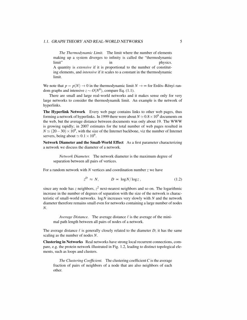
The Thermodynamic Limit. The limit where the number of elementsmaking up a system diverges to infinity is called the “thermodynamiclimit” in physics.A quantity is extensive if it is proportional to the number of constitut-ing elements, and intensive if it scales to a constant in the thermodynamiclimit.
We note that p = p(N)→ 0 in the thermodynamic limit N→ ∞ for Erdos–Renyi ran-dom graphs and intensive z∼ O(N0), compare Eq. (1.1).
There are small and large real-world networks and it makes sense only for verylarge networks to consider the thermodynamik limit. An example is the network ofhyperlinks.
The Hyperlink Network Every web page contains links to other web pages, thusforming a network of hyperlinks. In 1999 there were about N' 0.8×10⁹ documents onthe web, but the average distance between documents was only about 19. The WWWis growing rapidly; in 2007 estimates for the total number of web pages resulted inN ' (20−30)×109, with the size of the Internet backbone, viz the number of Internetservers, being about ' 0.1×10⁹.
Network Diameter and the Small-World Effect As a first parameter characterizinga network we discuss the diameter of a network.
Network Diameter. The network diameter is the maximum degree ofseparation between all pairs of vertices.
For a random network with N vertices and coordination number z we have
zD ≈ N, D ∝ logN/ logz , (1.2)
since any node has z neighbors, z2 next-nearest neighbors and so on. The logarithmicincrease in the number of degrees of separation with the size of the network is charac-teristic of small-world networks. logN increases very slowly with N and the networkdiameter therefore remains small even for networks containing a large number of nodesN.
Average Distance. The average distance ` is the average of the mini-mal path length between all pairs of nodes of a network.
The average distance ` is generally closely related to the diameter D; it has the samescaling as the number of nodes N.
Clustering in Networks Real networks have strong local recurrent connections, com-pare, e.g. the protein network illustrated in Fig. 1.2, leading to distinct topological ele-ments, such as loops and clusters.
The Clustering Coefficient. The clustering coefficient C is the averagefraction of pairs of neighbors of a node that are also neighbors of eachother.

6 CHAPTER 1. GRAPH THEORY AND SMALL-WORLD NETWORKS
The clustering coefficient is a normalized measure of loops of length 3. In a fullyconnected network, in which everyone knows everyone else, C = 1.
In a random graph a typical site has z(z− 1)/2 pairs of neighbors. The probabil-ity of an edge to be present between a given pair of neighbors is p = z/(N− 1), seeEq. (1.1). The clustering coefficient, which is just the probability of a pair of neighborsto be interconnected is therefore
Crand =z
N−1≈ z
N. (1.3)
It is very small for large random networks and scales to zero in the thermodynamiclimit. In Table 1.1 the respective clustering coefficients for some real-world networksand for the corresponding random networks are listed for comparison.Cliques and Communities The clustering coefficient measures the normalized num-ber of triples of fully interconnected vertices. In general, any fully connected subgraphis denoted a clique.
Cliques. A clique is a set of vertices for which (a) every node isconnected by an edge to every other member of the clique and (b) no nodeoutside the clique is connected to all members of the clique.
The term “clique” comes from social networks. A clique is a group of friends whereeverybody knows everybody else. The number of cliques of size K in an Erdos–Renyigraph with N vertices and linking probability p is(
NK
)pK(K−1)/2 (1− pK)N−K
.
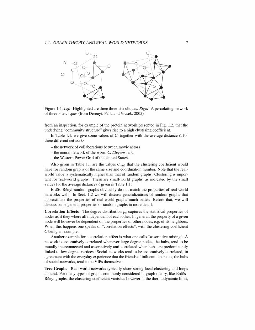
The only cliques occurring in random graphs in the thermodynamic limit have the size2, since p = z/N. For an illustration see Fig. 1.4.
Another term used is community. It is mathematically not as strictly defined as“clique”, it roughly denotes a collection of strongly overlapping cliques, viz of sub-graphs with above-the-average densities of edges.Clustering for Real-World Networks Most real-world networks have a substantialclustering coefficient, which is much greater than O(N−1). It is immediately evident
Table 1.1: The number of nodes N, average degree of separation `, and clusteringcoefficient C, for three real-world networks. The last column is the value which Cwould take in a random graph with the same size and coordination number, Crand = z/N(from Watts and Strogatz, 1998)
Network N ` C Crand
Movie actors 225226 3.65 0.79 0.00027Neural network 282 2.65 0.28 0.05Power grid 4941 18.7 0.08 0.0005
1.1. GRAPH THEORY AND REAL-WORLD NETWORKS 7
Figure 1.4: Left: Highlighted are three three-site cliques. Right: A percolating networkof three-site cliques (from Derenyi, Palla and Vicsek, 2005)
from an inspection, for example of the protein network presented in Fig. 1.2, that theunderlying “community structure” gives rise to a high clustering coefficient.
In Table 1.1, we give some values of C, together with the average distance `, forthree different networks:
– the network of collaborations between movie actors– the neural network of the worm C. Elegans, and– the Western Power Grid of the United States.
Also given in Table 1.1 are the values Crand that the clustering coefficient wouldhave for random graphs of the same size and coordination number. Note that the real-world value is systematically higher than that of random graphs. Clustering is impor-tant for real-world graphs. These are small-world graphs, as indicated by the smallvalues for the average distances ` given in Table 1.1.
Erdos–Renyi random graphs obviously do not match the properties of real-worldnetworks well. In Sect. 1.2 we will discuss generalizations of random graphs thatapproximate the properties of real-world graphs much better. Before that, we willdiscuss some general properties of random graphs in more detail.
Correlation Effects The degree distribution pk captures the statistical properties ofnodes as if they where all independent of each other. In general, the property of a givennode will however be dependent on the properties of other nodes, e.g. of its neighbors.When this happens one speaks of “correlation effects”, with the clustering coefficientC being an example.
Another example for a correlation effect is what one calls “assortative mixing”. Anetwork is assortatively correlated whenever large-degree nodes, the hubs, tend to bemutally interconnected and assortatively anti-correlated when hubs are predominantlylinked to low-degree vertices. Social networks tend to be assortatively correlated, inagreement with the everyday experience that the friends of influential persons, the hubsof social networks, tend to be VIPs themselves.
Tree Graphs Real-world networks typically show strong local clustering and loopsabound. For many types of graphs commonly considered in graph theory, like Erdos–Renyi graphs, the clustering coefficient vanishes however in the thermodynamic limit,

8 CHAPTER 1. GRAPH THEORY AND SMALL-WORLD NETWORKS
and loops become irrelevant. One denotes a loopless graph a “tree graph”, a conceptoften encountered in mathematical graph theory.Bipartite Networks Many real-world graphs have an underlying bipartite structure,see Fig. 1.1.
Bipartite Graph. A bipartite graph has two kinds of vertices withlinks only between vertices of unlike kinds.
Examples are networks of managers, where one kind of vertex is a company and theother kind of vertex the managers belonging to the board of directors. When elim-inating one kind of vertex, in this case it is customary to eliminate the companies,one retains a social network; the network of directors, as illustrated in Fig. 1.1. Thisnetwork has a high clustering coefficient, as all boards of directors are mapped ontocliques of the respective social network.
1.1.3 Properties of Random GraphsSo far we have considered mostly averaged quantities of random graphs, like the clus-tering coefficient or the average coordination number z. We will now develop toolsallowing for a more sophisticated characterization of graphs.Degree Distribution The basic description of general random and non-random graphsis given by the degree distribution pk.
Degree Distribution. If Xk is the number of vertices having the degreek, then pk = Xk/N is called the degree distribution, where N is the totalnumber of nodes.
The degree distribution is a probability distribution function and hence normalized,∑k pk = 1.Degree Distribution for Erdos–Renyi Graphs The probability of any node to havek edges is
pk =
(N−1
k
)pk (1− p)N−1−k , (1.4)
for an Erdos–Renyi network, where p is the link connection probability. For largeN k we can approximate the degree distribution pk by
pk ' e−pN (pN)k
k!= e−z zk
k!, (1.5)
where z is the average coordination number, compare Eq. (1.1). We have used
limN→∞
(1− x
N
)N= e−x,
(N−1
k
)=
(N−1)!k!(N−1− k)!
' (N−1)k
k!,
and (N− 1)k pk = zk, see Eq. (1.1). Equation (1.5) is a Poisson distribution with themean
〈k〉 =∞
∑k=0
k e−z zk
k!= ze−z
∞
∑k=1
zk−1
(k−1)!= z ,

1.1. GRAPH THEORY AND REAL-WORLD NETWORKS 9
as expected.
Ensemble Fluctuations In general, two specific realizations of random graphs differ.Their properties coincide on the average, but not on the level of individual links. With“ensemble” one denotes the set of possible realizations.
In an ensemble of random graphs with fixed p and N the degree distribution Xk/Nwill be slightly different from one realization to the next. On the average it will begiven by
1N〈Xk〉 = pk . (1.6)
Here 〈. . .〉 denotes the ensemble average. One can go one step further and calculatethe probability P(Xk = R) that in a realization of a random graph the number of verticeswith degree k equals R. It is given in the large-N limit by
P(Xk = R) = e−λk(λk)
R
R!, λk = 〈Xk〉 . (1.7)
Note the similarity to Eq. (1.5) and that the mean λk = 〈Xk〉 is in general extensivewhile the mean z of the degree distribution (1.5) is intensive.
Scale-Free Graphs Scale-free graphs are defined by a power-law degreedistribution
pk ∼1
kα, α > 1 . (1.8)
Typically, for real-world graphs, this scaling ∼ k−α holds only for large degrees k. Fortheoretical studies we will mostly assume, for simplicity, that the functional depen-dence Eq. (1.8) holds for all k. The power-law distribution can be normalized if
limK→∞
K
∑k=0
pk ≈ limK→∞
∫ K
k=0pk ∝ lim
K→∞K1−α < ∞ ,
i.e. when α > 1. The average degree is finite if
limK→∞
K
∑k=0
k pk ∝ limK→∞
K−α+2 < ∞ , α > 2 .
A power-law functional relation is called scale-free, since any rescaling k→ ak can bereabsorbed into the normalization constant.
Scale-free functional dependencies are also called critical, since they occur gener-ally at the critical point of a phase transition. We will come back to this issue recur-rently in the following chapters.
Graph Spectra Any graph G with N nodes can be represented by a matrix encodingthe topology of the network, the adjacency matrix.
The Adjacency Matrix. The N×N adjacency matrix A has elementsAi j = 1 if nodes i and j are connected and Ai j = 0 if they are not connected.
The adjacency matrix is symmetric and consequently has N real eigenvalues.
10 CHAPTER 1. GRAPH THEORY AND SMALL-WORLD NETWORKS
The Spectrum of a Graph. The spectrum of a graph G is given by theset of eigenvalues λi of the adjacency matrix A.
A graph with N nodes has N eigenvalues λi and it is useful to define the corresponding“spectral density”
ρ(λ ) =1N ∑
jδ (λ −λ j),
∫dλ ρ(λ ) = 1 , (1.9)
where δ (λ ) is the Dirac delta function.Green’s Function2
The spectral density ρ(λ ) can be evaluated once the Green’s function G(λ ),
G(λ ) =1N
Tr[
1λ − A
]=
1N ∑
j
1λ −λ j
, (1.10)
is known. Here Tr[. . .] denotes the trace over the matrix (λ − A)−1 ≡ (λ 1− A)−1,where 1 is the identity matrix. Using the formula
limε→0
1λ −λ j + iε
= P1
λ −λ j− iπδ (λ −λ j) ,
where P denotes the principal part,3 we find the relation
ρ(λ ) = − 1π
limε→0
ImG(λ + iε) . (1.11)
The Semi-Circle Law The graph spectra can be evaluated for random matrices forthe case of small link densities p = z/N, where z is the average connectivity. Startingfrom a random site we can connect on the average to z neighboring sites and from thereon to z−1 next-nearest neighboring sites, and so on:
G(λ ) =1
λ − zλ− z−1
λ− z−1λ−...
≈ 1λ − zG(λ )
, (1.12)
where we have approximated z− 1 ≈ z in the last step. Equation (1.12) is also calledthe “self-retracting path approximation” and can be derived by evoking a mapping toGreen’s function of a particle moving along the vertices of the graph. It constitutes aself-consistency equation for G = G(λ ), with the solution
G2− λ
zG+
1z= 0, G =
λ
2z−
√λ 2
4z2 −1z,
2The reader without prior experience with Green’s functions may skip the following derivation and passdirectly to the result, namely to Eq. (1.13).
3Taking the principal part signifies that one has to consider the positive and the negative contributionsto the 1/λ divergences carefully.

1.1. GRAPH THEORY AND REAL-WORLD NETWORKS 11
since limλ→∞ G(λ ) = 0. The spectral density Eq. (1.11) then takes the form
ρ(λ ) =
√4z−λ 2/(2πz) if λ 2 < 4z
0 if λ 2 > 4z(1.13)
of a half-ellipse also known as “Wigner’s law”, or the “semi-circle law”.Loops and the Clustering Coefficient The total number of triangles, viz the overallnumber of loops of length 3 in a network is C(N/3)(z−1)z/2, where C is the clusteringcoefficient. This number is related to the adjacency matrix via
CN3
z(z−1)2
= number of triangles
=16 ∑
i1,i2,i3
Ai1i2Ai2i3Ai3i1 =16
Tr[A3] ,
since three sites i1, i2 and i3 are interconnected only when the respective entries of theadjacency matrix are unity. The sum of the right-hand side of above relation is alsodenoted a “moment” of the graph spectrum. The factors 1/3 and 1/6 on the left-handside and on the right-hand side account for overcountings.Moments of the Spectral Density The graph spectrum is directly related to certaintopological features of a graph via its moments. The lth moment of ρ(λ ) is given by∫
dλ λlρ(λ ) =
1N
N
∑j=1
(λ j)l
=1N
Tr[Al]=
1N ∑
i1,i2,...,il
Ai1i2Ai2i3 · · ·Ail i1 , (1.14)
as one can see from Eq. (1.9). The lth moment of ρ(λ ) is therefore equivalent to thenumber of closed paths of length l, the number of all paths of length l returning to thestarting point.Graph Laplacian Consider a function f (x). The first and second derivatives aregiven by
ddx
f (x) =f (x+∆x)− f (x)
∆x,
d2
dx2 f (x) =f (x+∆x)+ f (x−∆x)−2 f (x)
∆x2 ,
in the limit ∆x→ 0. Consider now a function fi, i = 1, ...,N on a graph with N sites.One defines the graph Laplacian Λ via
Λi j =
(∑
jAi j
)δi j−Ai j =
ki i = j−1 i and j connected0 otherwise
, (1.15)
where the Λi j = (Λ)i j are the elements of the Laplacian matrix, Ai j the adjacency ma-trix, and where ki is the degree of vertex i. Λ corresponds, apart from a sign convention,to a straightforward generalization of the usual Laplace operator. To see this, just applythe Laplacian matrix Λi j to a graph-function f = ( f1, ..., fN).

12 CHAPTER 1. GRAPH THEORY AND SMALL-WORLD NETWORKS
Alternatively one defines by
Li j =
1 i = j
−1/√
ki k j i and j connected0 otherwise
, (1.16)
the “normalized graph Laplacian”, where ki = ∑ j Ai j is the degree of vertex i. Theeigenvalues of the normalized graph Laplacian have a straightforward interpretation interms of the underlying graph topology.Eigenvalues of the Normalized Graph Laplacian Of interest are the eigenvalues λl ,l = 0, ..,(N−1) of the normalized graph Laplacian.
– The normalized graph Laplacian is positive semidefinite,
0 = λ0 ≤ λ1 ≤ . . .≤ λN−1 ≤ 2 .
– The lowest eigenvalue λ0 is always zero, corresponding to the eigenfunction
e(λ0) =1√C
(√k1,√
k2, . . . ,√
kN
), (1.17)
where C is a normalization constant and where the ki are the respective vertex-degrees.
– The degeneracy of λ0 is given by the number of disconnected subgraphs con-tained in the network. The eigenfunctions of λ0 then vanish on all subclustersbeside one, where it has the functional form (1.17).
– The largest eigenvalue λN−1 is λN−1 = 2, if and only if the network is bipartite.Generally, a small value of 2−λN−1 indicates that the graph is nearly bipartite.
– The inequality∑
lλl ≤ N
holds generally. The equality holds for connected graphs, viz when λ0 has de-generacy one.
Examples of Graph Laplacians The eigenvalues of the normalized graph Laplaciancan be given analytically for some simple graphs.
• For a complete graph (all sites are mutually interconnected), containing N sites,the eigenvalues are
λ0 = 0, λl = N/(N−1), (l = 1, ...,N−1) .
• For a complete bipartite graph (all sites of one subgraph are connected to allother sites of the other subgraph) the eigenvalues are
λ0 = 0, λN−1 = 2, λl = 1, (l = 1, ...,N−2) .

1.2. GENERALIZED RANDOM GRAPHS 13
The eigenfunction for λN−1 = 2 has the form
e(λN−1) =1√C
(√kA, . . . ,
√kA︸ ︷︷ ︸
A sublattice
,−√
kB, . . . ,−√
kB︸ ︷︷ ︸B sublattice
). (1.18)
Denoting with NA and NB the number of sites in two sublattices A and B, withNA +NB = N, the degrees kA and kB of vertices belonging to sublattice A and Brespectively are kA = NB and kB = NA for a complete bipartite lattice.
A densely connected graph will therefore have many eigenvalues close to unity.For real-world graphs one may therefore plot the spectral density of the normalizedgraph Laplacian in order to gain an insight into its overall topological properties. Theinformation obtained from the spectral density of the adjacency matrix and from thenormalized graph Laplacian are distinct.
1.2 Generalized Random GraphsThe most random of all graphs are Erdos–Renyi graphs. One can relax the degreeof randomness somewhat and construct random networks having an arbitrarily givendegree distribution. This procedure is also denoted “configurational model”.
1.2.1 Graphs with Arbitrary Degree DistributionsIn order to generate random graphs that have non-Poisson degree distributions we maychoose a specific set of degrees.
The Degree Sequence. A degree sequence is a specified set ki ofthe degrees for the vertices i = 1 . . .N.
Construction of Networks with Arbitrary Degree Distribution The degree se-quence can be chosen in such a way that the fraction of vertices having degree k willtend to the desired degree distribution
pk, N→ ∞
in the thermodynamic limit. The network can then be constructed in the following way:
1. Assign ki “stubs” (ends of edges emerging from a vertex) to every vertex i =1, . . . ,N.
2. Iteratively choose pairs of stubs at random and join them together to make com-plete edges.
When all stubs have been used up, the resulting graph is a random member of theensemble of graphs with the desired degree sequence. Figure 1.5 illustrates the con-struction procedure.The Average Degree and Clustering The mean number of neighbors is the coordi-nation number
z = 〈k〉 = ∑k
k pk .

14 CHAPTER 1. GRAPH THEORY AND SMALL-WORLD NETWORKS
Step A Step B
Figure 1.5: Construction procedure of a random network with nine vertices and degreesX1 = 2, X2 = 3, X3 = 2, X4 = 2. In step A the vertices with the desired number of stubs(degrees) are constructed. In step B the stubs are connected randomly
The probability that one of the second neighbors of a given vertex is also a first neigh-bor, scales as N−1 for random graphs, regardless of the degree distribution, and hencecan be ignored in the limit N→ ∞.
Degree Distribution of Neighbors Consider a given vertex A and a vertex B that is aneighbor of A, i.e. A and B are linked by an edge.
We are now interested in the degree distribution for vertex B, viz in the degreedistribution of a neighbor vertex of A, where A is an arbitrary vertex of the randomnetwork with degree distribution pk. As a first step we consider the average degree ofa neighbor node.
A high-degree vertex has more edges connected to it. There is then a higher chancethat any given edge on the graph will be connected to it, with this chance being directlyproportional to the degree of the vertex. Thus the probability distribution of the degreeof the vertex to which an edge leads is proportional to kpk and not just to pk.
Excess Degree Distribution When we are interested in determining the size of loopsor the size of connected components in a random graph, we are normally interested notin the complete degree of the vertex reached by following an edge from A, but in thenumber of edges emerging from such a vertex that do not lead back to A, because thelatter contains all information about the number of second neighbors of A.
The number of new edges emerging from B is just the degree of B minus one andits correctly normalized distribution is therefore
qk−1 =k pk
∑ j jp j, qk =
(k+1)pk+1
∑ j jp j, (1.19)
since kpk is the degree distribution of a neighbor. The distribution qk of the outgoingedges of a neighbor vertex is also denoted “excess degree distribution”. The averagenumber of outgoing edges of a neighbor vertex is then
∞
∑k=0
kqk =∑
∞k=0 k(k+1)pk+1
∑ j jp j=
∑∞k=1(k−1)kpk
∑ j jp j
=〈k2〉−〈k〉〈k〉
. (1.20)

1.2. GENERALIZED RANDOM GRAPHS 15
Number of Next-Nearest Neighbors We denote with
zm, z1 = 〈k〉 ≡ z
the average number of m-nearest neighbors. Equation (1.20) gives the average numberof vertices two steps away from the starting vertex A via a particular neighbor vertex.Multiplying this by the mean degree of A, namely z1 ≡ z, we find that the mean numberof second neighbors z2 of a vertex is
z2 = 〈k2〉−〈k〉 . (1.21)
z2 for the Erdos–Renyi graph The degree distribution of an Erdos–Renyi graph is thePoisson distribution, pk = e−z zk/k!, see Eq. (1.5). We obtain for the average numberof second neighbors, Eq. (1.21),
z2 =∞
∑k=0
k2e−z zk
k!− z = ze−z
∞
∑k=1
(k−1+1)zk−1
(k−1)!− z
= z2 = 〈k〉2 .The mean number of second neighbors of a vertex in an Erdos–Renyi random graph isjust the square of the mean number of first neighbors. This is a special case however.For most degree distributions, Eq. (1.21) will be dominated by the term 〈k2〉, so thenumber of second neighbors is roughly the mean square degree, rather than the squareof the mean. For broad distributions these two quantities can be very different.Number of Far Away Neighbors The average number of edges emerging from a sec-ond neighbor, and not leading back to where we came from, is also given by Eq. (1.20),and indeed this is true at any distance m away from vertex A. The average number ofneighbors at a distance m is then
zm =〈k2〉−〈k〉〈k〉
zm−1 =z2
z1zm−1 , (1.22)
where z1 ≡ z = 〈k〉 and z2 are given by Eq. (1.21). Iterating this relation we find
zm =
[z2
z1
]m−1
z1 . (1.23)
The Giant Connected Cluster Depending on whether z2 is greater than z1 or not,Eq. (1.23) will either diverge or converge exponentially as m becomes large:
limm→∞
zm =
∞ if z2 > z10 if z2 < z1
, (1.24)
z1 = z2 is the percolation point. In the second case the total number of neighbors
∑m
zm = z1
∞
∑m=1
[z2
z1
]m−1
=z1
1− z2/z1=
z21
z1− z2
is finite even in the thermodynamic limit, in the first case it is infinite. The network de-cays, for N→ ∞, into non-connected components when the total number of neighborsis finite.

16 CHAPTER 1. GRAPH THEORY AND SMALL-WORLD NETWORKS
The Giant Connected Component. When the largest cluster of a graphencompasses a finite fraction of all vertices, in the thermodynamic limit, itis said to form a giant connected component (GCC).
If the total number of neighbors is infinite, then there must be a giant connected compo-nent. When the total number of neighbors is finite, there can be noGCC.The Percolation Threshold When a system has two or more possibly macroscopi-cally different states, one speaks of a phase transition.
Percolation Transition. When the structure of an evolving graph goesfrom a state in which two (far away) sites are on the average connected/notconnected one speaks of a percolation transition.
This phase transition occurs precisely at the point where z2 = z1. Making use ofEq. (1.21), z2 = 〈k2〉−〈k〉, we find that this condition is equivalent to
〈k2〉−2〈k〉 = 0,∞
∑k=0
k(k−2)pk = 0 . (1.25)
We note that, because of the factor k(k−2), vertices of degree zero and degree twodo not contribute to the sum. The number of vertices with degree zero or two thereforeaffects neither the phase transition nor the existence of the giant component.
– Vertices of degree zero are not connected to any other node, they do not con-tribute to the network topology.
– Vertices of degree two act as intermediators between two other nodes. Removingvertices of degree two does not change the topological structure of a graph.
One can therefore remove (or add) vertices of degree two or zero without affecting theexistence of the giant component.Clique Percolation Edges correspond to cliques with Z = 2 sites (see page 6). Thepercolation transition can then also be interpreted as a percolation of cliques havingsize two and larger. It is then clear that the concept of percolation can be generalizedto that of percolation of cliques with Z sites, see Fig. 1.4 for an illustration.The Average Vertex–Vertex Distance Below the percolation threshold the averagevertex–vertex distance ` is finite and the graph decomposes into an infinite number ofdisconnected subclusters.
Disconnected Subclusters. A disconnected subcluster or subgraphconstitutes a subset of vertices for which (a) there is at least one path inbetween all pairs of nodes making up the subcluster and (b) there is no pathbetween a member of the subcluster and any out-of-subcluster vertex.
Well above the percolation transition, ` is given approximately by the conditionz` ' N:
log(N/z1) = (`−1) log(z2/z1), ` =log(N/z1)
log(z2/z1)+1 , (1.26)
1.2. GENERALIZED RANDOM GRAPHS 17
using Eq. (1.23). For the special case of the Erdos–Renyi random graph, for whichz1 = z and z2 = z2, this expression reduces to the standard formula (1.2),
` =logN− logz
logz+ 1 =
logNlogz
.
The Clustering Coefficient of Generalized Random Graphs The clustering coef-ficient C denotes the probability that two neighbors i and j of a particular vertex Ahave stubs that do interconnect. The probability that two given stubs are connectedis 1/(zN− 1) ≈ 1/zN, since zN is the total number of stubs. We then have, compareEq. (1.20),
C =〈kik j〉q
Nz=〈ki〉q〈k j〉q
Nz=
1Nz
[∑k
kqk
]2
=1
Nz
[〈k2〉−〈k〉〈k〉
]2
=zN
[〈k2〉−〈k〉〈k〉2
]2
, (1.27)
since the distributions of two neighbors i and j are statistically independent. The no-tation 〈...〉q indicates that the average is to be take with respect to the excess degreedistribution qk, as given by Eq. (1.19).
The clustering coefficient vanishes in the thermodynamic limit N→∞, as expected.However, it may have a very big leading coefficient, especially for degree distributionswith fat tails. The differences listed in Table 1.1, between the measured clusteringcoefficient C and the value Crand = z/N for Erdos–Renyi graphs, are partly due to thefat tails in the degree distributions pk of the corresponding networks.
1.2.2 Probability Generating Function Formalism
Network theory is about the statistical properties of graphs. A very powerful methodfrom probability theory is the generating function formalism, which we will discussnow and apply later on.
Probability Generating Functions We define by
G0(x) =∞
∑k=0
pkxk (1.28)
the generating function G0(x) for the probability distribution pk. The generating func-tion G0(x) contains all information present in pk. We can recover pk from G0(x) simplyby differentiation:
pk =1k!
dkG0
dxk
∣∣∣∣x=0
. (1.29)
One says that the function G0 “generates” the probability distribution pk.
The Generating Function for Degree Distribution of Neighbors We can also definea generating function for the distribution qk, Eq. (1.19), of the other edges leaving a

18 CHAPTER 1. GRAPH THEORY AND SMALL-WORLD NETWORKS
vertex that we reach by following an edge in the graph:
G1(x) =∞
∑k=0
qkxk =∑
∞k=0(k+1)pk+1xk
∑ j jp j=
∑∞k=0 kpkxk−1
∑ j jp j
=G′0(x)
z, (1.30)
where G′0(x) denotes the first derivative of G0(x) with respect to its argument.Properties of Generating Functions Probability generating functions have a coupleof important properties:
1. Normalization: The distribution pk is normalized and hence
G0(1) = ∑k
pk = 1 . (1.31)
2. Mean: A simple differentiation
G′0(1) = ∑k
k pk = 〈k〉 (1.32)
yields the average degree 〈k〉.
3. Moments: The nth moment 〈kn〉 of the distribution pk is given by
〈kn〉 = ∑k
kn pk =
[(x
ddx
)n
G0(x)]
x=1. (1.33)
The Generating Function for Independent Random Variables Let us assume thatwe have two random variables. As an example we consider two dice. Throwing the twodice are two independent random events. The joint probability to obtain k = 1, . . . ,6with the first die and l = 1, . . . ,6 with the second dice is pk pl . This probability functionis generated by
∑k,l
pk pl xk+l =
(∑k
pk xk
)(∑
lpl xl
),
i.e. by the product of the individual generating functions. This is the reason why gener-ating functions are so useful in describing combinations of independent random events.
As an application consider n randomly chosen vertices. The sum ∑i ki of the re-spective degrees has a cumulative degree distribution, which is generated by[
G0(x)]n.
The Generating Function of the Poisson Distribution As an example we considerthe Poisson distribution pk = e−z zk/k!, see Eq. (1.5), with z being the average degree.Using Eq. (1.28) we obtain
G0(x) = e−z∞
∑k=0
zk
k!xk = ez(x−1) . (1.34)
1.2. GENERALIZED RANDOM GRAPHS 19
This is the generating function for the Poisson distribution. The generating functionG1(x) for the excess degree distribution qk is, see Eq. (1.30),
G1(x) =G′0(x)
z= ez(x−1) . (1.35)
Thus, for the case of the Poisson distribution we have, as expected, G1(x) = G0(x).Further Examples of Generating Functions As a second example, consider a graphwith an exponential degree distribution:
pk = (1− e−1/κ)e−k/κ ,∞
∑k=0
pk =1− e−1/κ
1− e−1/κ= 1 , (1.36)
where κ is a constant. The generating function for this distribution is
G0(x) = (1− e−1/κ)∞
∑k=0
e−k/κ xk =1− e−1/κ
1− xe−1/κ, (1.37)
and
z = G′0(1) =e−1/κ
1− e−1/κ, G1(x) =
G′0(x)z
=
[1− e−1/κ
1− xe−1/κ
]2
. (1.38)
As a third example, consider a graph in which all vertices have degree 0, 1, 2,or 3 with probabilities p0 . . . p3. Then the generating functions take the form of simplepolynomials
G0(x) = p3x3 + p2x2 + p1x+ p0, (1.39)
G1(x) = q2x2 +q1x+q0 =3p3x2 +2p2x+ p1
3p3 +2p2 + p1. (1.40)
Stochastic Sum of Independent Variables Let’s assume we have random variablesk1, k2, . . ., each having the same generating functional G0(x). Then
G20 (x), G3
0 (x), G40 (x), . . .
are the generating functionals for
k1 + k2, k1 + k2 + k3, k1 + k2 + k3 + k4, . . . .
Now consider that the number of times n this stochastic prozess is executed is dis-tributed as pn. As an example consider throwing a dice several times, with a probablitypn of throwing exacly n times. The distribution of the results obtained is then generatedby
∑n
pnGn0 (x) = GN (G0(x)) , GN(z) = ∑
npnzn . (1.41)
We will make use of this relation further on.

20 CHAPTER 1. GRAPH THEORY AND SMALL-WORLD NETWORKS
. . .+++= +
Figure 1.6: Graphical representation of the self-consistency Eq. (1.42) for the generat-ing function H1(x), represented by the box. A single vertex is represented by a circle.The subcluster connected to an incoming vertex can be either a single vertex or anarbitrary number of subclusters of the same type connected to the first vertex (fromNewman et al., 2001)
1.2.3 Distribution of Component Sizes
The Absence of Closed Loops We consider here a network below the percola-tion transition and are interested in the distribution of the sizes of the individual sub-clusters. The calculations will crucially depend on the fact that the generalized ran-dom graphs considered here do not have any significant clustering nor any closedloops.
Closed Loops. A set of edges linking vertices
i1→ i2 . . . in→ i1
is called a closed loop of length n.
In physics jargon, all finite components are tree-like. The number of closed loops oflength 3 corresponds to the clustering coefficient C, viz to the probability that twoof your friends are also friends of each other. For random networks C = [〈k2〉 −〈k〉]2/(z3N), see Eq. (1.27), tends to zero as N→ ∞.Generating Function for the Size Distribution of Components We define by
H1(x) = ∑m
h(1)m xm
the generating function that generates the distribution of cluster sizes containing a givenvertex j, which is linked to a specific incoming edge, see Fig. 1.6. That is, h(1)m is theprobability that the such-defined cluster contains m nodes.Self-Consistency Condition for H1(x) We note the following:
1. The first vertex j belongs to the subcluster with probability 1, its generatingfunction is x.
2. The probability that the vertex j has k outgoing stubs is qk.
3. At every stub outgoing from vertex j there is a subcluster.
4. The total number of vertices consists of those generated by H1(x) plus the start-ing vertex.

1.2. GENERALIZED RANDOM GRAPHS 21
The number of outgoing edges k from vertex j is described by the distribution functionqk, see Eq. (1.19). The total size of the k clusters is generated by [H1(x)]k, as a conse-quence of the multiplication property of generating functions discussed in Sect. 1.2.2.The self-consistency equation for the total number of vertices reachable is then
H1(x) = x∞
∑k=0
qk [H1(x)]k = xG1(H1(x)) , (1.42)
where we have made use of Eqs. (1.30) and (1.41).The Embedding Cluster Distribution Function The quantity that we actually wantto know is the distribution of the sizes of the clusters to which the entry vertex belongs.We note that
1. The number of edges emanating from a randomly chosen vertex is distributedaccording to the degree distribution pk.
2. Every edge leads to a cluster whose size is generated by H1(x).
The size of a complete component is thus generated by
H0(x) = x∞
∑k=0
pk [H1(x)]k = xG0(H1(x)) , (1.43)
where the prefactor x corresponds to the generating function of the starting vertex.The complete distribution of component sizes is given by solving Eq. (1.42) self-consistently for H1(x) and then substituting the result into Eq. (1.43).The Mean Component Size The calculation of H1(x) and H0(x) in closed form is notpossible. We are, however, interested only in the first moment, viz the mean componentsize, see Eq. (1.32).
The component size distribution is generated by H0(x), Eq. (1.43), and hence themean component size below the percolation transition is
〈s〉 = H ′0(1) =[
G0(H1(x))+ xG′0(H1(x))H ′1(x)]
x=1
= 1+G′0(1)H′1(1) , (1.44)
where we have made use of the normalization
G0(1) = H1(1) = H0(1) = 1 .
of generating functions, see Eq. (1.31). The value of H ′1(1) can be calculated fromEq. (1.42) by differentiating:
H ′1(x) = G1(H1(x)) + xG′1(H1(x))H ′1(x), (1.45)
H ′1(1) =1
1−G′1(1).
Substituting this into (1.44) we find
〈s〉 = 1+G′0(1)
1−G′1(1). (1.46)
22 CHAPTER 1. GRAPH THEORY AND SMALL-WORLD NETWORKS
We note that
G′0(1) = ∑k
k pk = 〈k〉 = z1, (1.47)
G′1(1) =∑k k(k−1)pk
∑k kpk=〈k2〉−〈k〉〈k〉
=z2
z1,
where we have made use of Eq. (1.21). Substitution into (1.46) then gives the averagecomponent size below the transition as
〈s〉 = 1+z2
1z1− z2
. (1.48)
This expression has a divergence at z1 = z2. The mean component size diverges at thepercolation threshold, compare Sect. 1.2, and the giant connected component forms.
1.3 Robustness of Random NetworksFat tails in the degree distributions pk of real-world networks (only slowly decayingwith large k) increase the robustness of the network. That is, the network retains func-tionality even when a certain number of vertices or edges is removed. The Internetremains functional, to give an example, even when a substantial number of Internetrouters have failed.Removal of Vertices We consider a graph model in which each vertex is either “ac-tive” or “inactive”. Inactive vertices are nodes that have either been removed, or arepresent but non-functional. We denote by
b(k) = bk
the probability that a vertex is active. The probability can be, in general, a function ofthe degree k. The generating function
F0(x) =∞
∑k=0
pk bk xk, F0(1) = ∑k
pk bk ≤ 1 , (1.49)
generates the probabilities that a vertex has degree k and is present. The normalizationF0(1) is equal to the fraction of all vertices that are present. By analogy with Eq. (1.30)we define by
F1(x) =∑k k pk bk xk−1
∑k k pk=
F ′0(x)z
(1.50)
the (non-normalized) generating function for the degree distribution of neighbor sites.Distribution of Connected Clusters The distribution of the sizes of connected clus-ters reachable from a given vertex, H0(x), or from a given edge, H1(x), is generatedrespectively by the normalized functions
H0(x) = 1 − F0(1) + xF0(H1(x)), H0(1) = 1,H1(x) = 1 − F1(1) + xF1(H1(x)), H1(1) = 1 , (1.51)

1.3. ROBUSTNESS OF RANDOM NETWORKS 23
which are logical equivalents of Eqs. (1.42) and (1.43).Random Failure of Vertices First we consider the case of random failure of vertices.In this case, the probability
bk ≡ b ≤ 1, F0(x) = bG0(x), F1(x) = bG1(x)
of a vertex being present is independent of the degree k and just equal to a constant b,which means that
H0(x) = 1−b+bxG0(H1(x)), H1(x) = 1−b+bxG1(H1(x)), (1.52)
where G0(x) and G1(x) are the standard generating functions for the degree of a vertexand of a neighboring vertex, Eqs. (1.28) and (1.30). This implies that the mean size ofa cluster of connected and present vertices is
〈s〉 = H ′0(1) = b + bG′0(1)H ′1(1) = b +b2G′0(1)
1−bG′1(1)= b
[1+
bG′0(1)1−bG′1(1)
],
where we have followed the derivation presented in Eq. (1.45) in order to obtain H ′1(1)=b/(1−bG′1(1)). With Eq. (1.47) for G′0(1) = z1 = z and G′1(1) = z2/z1 we obtain thegeneralization
〈s〉 = b+b2z2
1z1−bz2
(1.53)
of Eq. (1.48). The model has a phase transition at the critical value of b
bc =z1
z2=
1G′1(1)
. (1.54)
If the fraction b of the vertices present in the network is smaller than the critical fractionbc, then there will be no giant component. This is the point at which the network ceasesto be functional in terms of connectivity. When there is no giant component, connectingpaths exist only within small isolated groups of vertices, but no long-range connectivityexists. For a communication network such as the Internet, this would be fatal.
For networks with fat tails, however, we expect that the number of next-nearestneighbors z2 is large compared to the number of nearest neighbors z1 and that bc isconsequently small. The network is robust as one would need to take out a substantialfraction of the nodes before it would fail.Random Failure of Vertices in Scale-Free Graphs We consider a pure power-lawdegree distribution
pk ∼1
kα,
∫ dkkα
< ∞, α > 1 ,
see Eq. (1.8) and also Sect. 1.5. The first two moments are
z1 = 〈k〉 ∼∫
dk (k/kα), 〈k2〉 ∼∫
dk (k2/kα) .
24 CHAPTER 1. GRAPH THEORY AND SMALL-WORLD NETWORKS
Noting that the number of next-nearest neighbors z2 = 〈k2〉− 〈k〉, Eq. (1.21), we canidentify three regimes:
– 1< α ≤ 2: z1→ ∞, z2→ ∞
bc = z1/z2 is arbitrary in the thermodynamic limit N→ ∞.
– 2< α ≤ 3: z1 < ∞, z2→ ∞
bc = z1/z2 → 0 in the thermodynamic limit. Any number of vertices can berandomly removed with the network remaining above the percolation limit. Thenetwork is extremely robust.
– 3< α: z1 < ∞, z2 < ∞
bc = z1/z2 can acquire any value and the network has normal robustness.
Biased Failure of Vertices What happens when one sabotages the most importantsites of a network? This is equivalent to removing vertices in decreasing order of theirdegrees, starting with the highest degree vertices. The probability that a given node isactive then takes the form
bk = θ(kc− k) , (1.55)
where θ(x) is the Heaviside step function
θ(x) =
0 for x< 01 for x≥ 0 . (1.56)
This corresponds to setting the upper limit of the sum in Eq. (1.49) to kc.Differentiating Eq. (1.51) with respect to x yields
H ′1(1) = F1(H1(1)) + F ′1(H1(1))H ′1(1), H ′1(1) =F1(1)
1−F ′1(1),
as H1(1) = 1. The phase transition occurs when F ′1(1) = 1,
∑∞k=1 k(k−1)pkbk
∑∞k=1 kpk
=∑
kck=1 k(k−1)pk
∑∞k=1 kpk
= 1 , (1.57)
where we used the definition Eq. (1.50) for F1(x).
Biased Failure of Vertices for Scale-Free Networks Scale-free networks have apower-law degree distribution, pk ∝ k−α . We can then rewrite Eq. (1.57) as
H(α−2)kc
− H(α−1)kc
= H(α−1)∞ , (1.58)
where H(r)n is the nth harmonic number of order r:
H(r)n =
n
∑k=1
1kr . (1.59)

1.3. ROBUSTNESS OF RANDOM NETWORKS 25
2.0 2.5 3.0 3.5
exponent α
0.00
0.01
0.02
0.03
crit
ical
fra
ctio
n f c
Figure 1.7: The critical fraction fc of vertices, Eq. (1.60). Removing a fraction greaterthan fc of highest degree vertices from a scale-free network, with a power-law degreedistribution pk ∼ k−α drives the network below the percolation limit. For a smaller lossof highest degree vertices (shaded area) the giant connected component remains intact(from Newman, 2002)
The number of vertices present is F0(1), see Eq. (1.49), or F0(1)/∑k pk, since thedegree distribution pk is normalized. If we remove a certain fraction fc of the verticeswe reach the transition determined by Eq. (1.58):
fc = 1 − F0(1)∑k pk
= 1 −H(α)
kc
H(α)∞
. (1.60)
It is impossible to determine kc from (1.58) and (1.60) to get fc in closed form. Onecan, however, solve Eq. (1.58) numerically for kc and substitute it into Eq. (1.60). Theresults are shown in Fig. 1.7, as a function of the exponent α . The network is verysusceptible with respect to a biased removal of highest-degree vertices.
– A removal of more than about 3% of the highest degree vertices always leads toa destruction of the giant connected component. Maximal robustness is achievedfor α ≈ 2.2, which is actually close to the exponents measured in some real-world networks.
– Networks with α < 2 have no finite mean, ∑k k/k2 → ∞, and therefore makelittle sense physically.
– Networks with α > αc = 3.4788. . . have no giant connected component. Thecritical exponent αc is given by the percolation condition H(α−2)
∞ = 2H(α−1)∞ , see
Eq. (1.25).
26 CHAPTER 1. GRAPH THEORY AND SMALL-WORLD NETWORKS
z = 4
z = 2
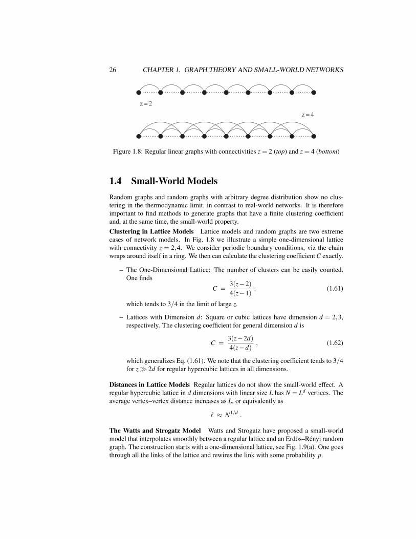
Figure 1.8: Regular linear graphs with connectivities z = 2 (top) and z = 4 (bottom)
1.4 Small-World ModelsRandom graphs and random graphs with arbitrary degree distribution show no clus-tering in the thermodynamic limit, in contrast to real-world networks. It is thereforeimportant to find methods to generate graphs that have a finite clustering coefficientand, at the same time, the small-world property.Clustering in Lattice Models Lattice models and random graphs are two extremecases of network models. In Fig. 1.8 we illustrate a simple one-dimensional latticewith connectivity z = 2,4. We consider periodic boundary conditions, viz the chainwraps around itself in a ring. We then can calculate the clustering coefficient C exactly.
– The One-Dimensional Lattice: The number of clusters can be easily counted.One finds
C =3(z−2)4(z−1)
, (1.61)
which tends to 3/4 in the limit of large z.
– Lattices with Dimension d: Square or cubic lattices have dimension d = 2,3,respectively. The clustering coefficient for general dimension d is
C =3(z−2d)4(z−d)
, (1.62)
which generalizes Eq. (1.61). We note that the clustering coefficient tends to 3/4for z 2d for regular hypercubic lattices in all dimensions.
Distances in Lattice Models Regular lattices do not show the small-world effect. Aregular hypercubic lattice in d dimensions with linear size L has N = Ld vertices. Theaverage vertex–vertex distance increases as L, or equivalently as
` ≈ N1/d .
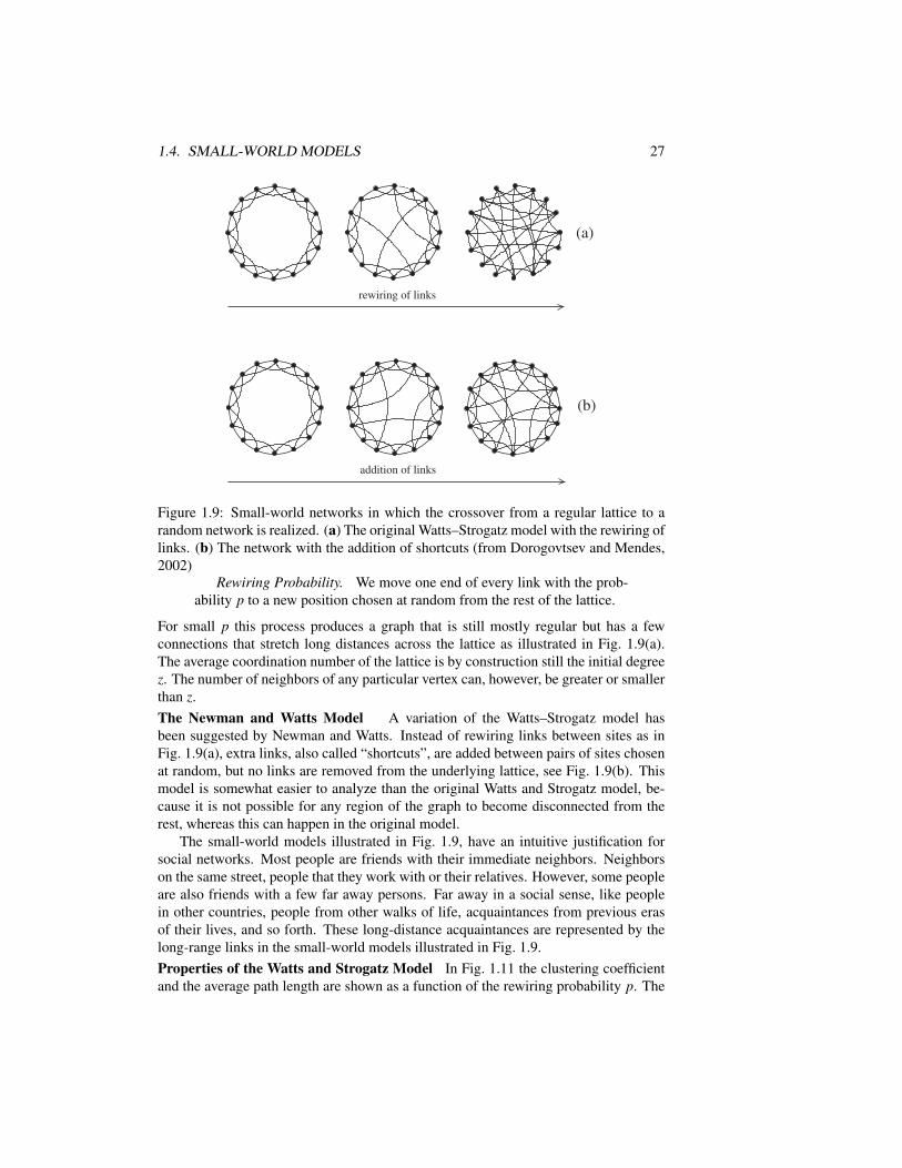
The Watts and Strogatz Model Watts and Strogatz have proposed a small-worldmodel that interpolates smoothly between a regular lattice and an Erdos–Renyi randomgraph. The construction starts with a one-dimensional lattice, see Fig. 1.9(a). One goesthrough all the links of the lattice and rewires the link with some probability p.
1.4. SMALL-WORLD MODELS 27
(a)
rewiring of links
(b)
addition of links
Figure 1.9: Small-world networks in which the crossover from a regular lattice to arandom network is realized. (a) The original Watts–Strogatz model with the rewiring oflinks. (b) The network with the addition of shortcuts (from Dorogovtsev and Mendes,2002)
Rewiring Probability. We move one end of every link with the prob-ability p to a new position chosen at random from the rest of the lattice.
For small p this process produces a graph that is still mostly regular but has a fewconnections that stretch long distances across the lattice as illustrated in Fig. 1.9(a).The average coordination number of the lattice is by construction still the initial degreez. The number of neighbors of any particular vertex can, however, be greater or smallerthan z.The Newman and Watts Model A variation of the Watts–Strogatz model hasbeen suggested by Newman and Watts. Instead of rewiring links between sites as inFig. 1.9(a), extra links, also called “shortcuts”, are added between pairs of sites chosenat random, but no links are removed from the underlying lattice, see Fig. 1.9(b). Thismodel is somewhat easier to analyze than the original Watts and Strogatz model, be-cause it is not possible for any region of the graph to become disconnected from therest, whereas this can happen in the original model.
The small-world models illustrated in Fig. 1.9, have an intuitive justification forsocial networks. Most people are friends with their immediate neighbors. Neighborson the same street, people that they work with or their relatives. However, some peopleare also friends with a few far away persons. Far away in a social sense, like peoplein other countries, people from other walks of life, acquaintances from previous erasof their lives, and so forth. These long-distance acquaintances are represented by thelong-range links in the small-world models illustrated in Fig. 1.9.Properties of the Watts and Strogatz Model In Fig. 1.11 the clustering coefficientand the average path length are shown as a function of the rewiring probability p. The
28 CHAPTER 1. GRAPH THEORY AND SMALL-WORLD NETWORKS
Figure 1.10: [
t]
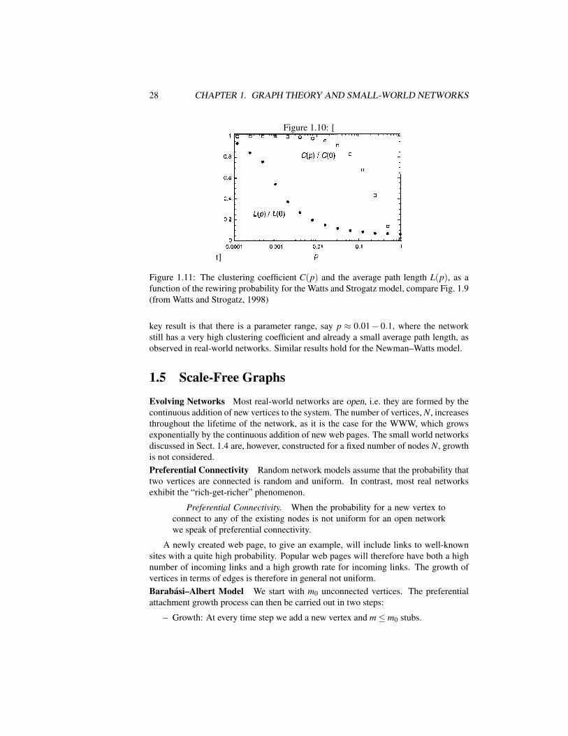
Figure 1.11: The clustering coefficient C(p) and the average path length L(p), as afunction of the rewiring probability for the Watts and Strogatz model, compare Fig. 1.9(from Watts and Strogatz, 1998)
key result is that there is a parameter range, say p ≈ 0.01− 0.1, where the networkstill has a very high clustering coefficient and already a small average path length, asobserved in real-world networks. Similar results hold for the Newman–Watts model.
1.5 Scale-Free Graphs
Evolving Networks Most real-world networks are open, i.e. they are formed by thecontinuous addition of new vertices to the system. The number of vertices, N, increasesthroughout the lifetime of the network, as it is the case for the WWW, which growsexponentially by the continuous addition of new web pages. The small world networksdiscussed in Sect. 1.4 are, however, constructed for a fixed number of nodes N, growthis not considered.Preferential Connectivity Random network models assume that the probability thattwo vertices are connected is random and uniform. In contrast, most real networksexhibit the “rich-get-richer” phenomenon.
Preferential Connectivity. When the probability for a new vertex toconnect to any of the existing nodes is not uniform for an open networkwe speak of preferential connectivity.
A newly created web page, to give an example, will include links to well-knownsites with a quite high probability. Popular web pages will therefore have both a highnumber of incoming links and a high growth rate for incoming links. The growth ofvertices in terms of edges is therefore in general not uniform.Barabasi–Albert Model We start with m0 unconnected vertices. The preferentialattachment growth process can then be carried out in two steps:
– Growth: At every time step we add a new vertex and m≤ m0 stubs.
1.5. SCALE-FREE GRAPHS 29
t = 0 t = 1 t = 2 t = 3
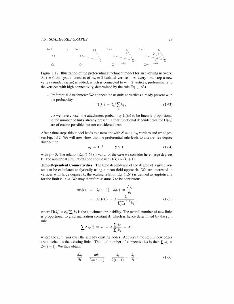
Figure 1.12: Illustration of the preferential attachment model for an evolving network.At t = 0 the system consists of m0 = 3 isolated vertices. At every time step a newvertex (shaded circle) is added, which is connected to m = 2 vertices, preferentially tothe vertices with high connectivity, determined by the rule Eq. (1.63)
– Preferential Attachment: We connect the m stubs to vertices already present withthe probability
Π(ki) = ki/∑j
k j , (1.63)
viz we have chosen the attachment probability Π(ki) to be linearly proportionalto the number of links already present. Other functional dependencies for Π(ki)are of course possible, but not considered here.
After t time steps this model leads to a network with N = t +m0 vertices and mt edges,see Fig. 1.12. We will now show that the preferential rule leads to a scale-free degreedistribution
pk ∼ k−γγ > 1 , (1.64)
with γ = 3. The relation Eq. (1.63) is valid for the case we consider here, large degreeski. For numerical simulations one should use Π(ki) ∝ (ki +1).
Time-Dependent Connectivities The time dependence of the degree of a given ver-tex can be calculated analytically using a mean-field approach. We are interested invertices with large degrees k; the scaling relation Eq. (1.64) is defined asymptoticallyfor the limit k→ ∞. We may therefore assume k to be continuous:
∆ki(t) ≡ ki(t +1)− ki(t) ≈∂ki
∂ t
= AΠ(ki) = Aki
∑m0+t−1j=1 k j
, (1.65)
where Π(ki) = ki/∑ j k j is the attachment probability. The overall number of new linksis proportional to a normalization constant A, which is hence determined by the sumrule
∑i
∆ki(t) ≡ m = A∑i ki
∑ j k j= A ,
where the sum runs over the already existing nodes. At every time step m new edgesare attached to the existing links. The total number of connectivities is then ∑ j k j =2m(t−1). We thus obtain
∂ki
∂ t=
mki
2m(t−1)=
ki
2(t−1)≈ ki
2t. (1.66)

30 CHAPTER 1. GRAPH THEORY AND SMALL-WORLD NETWORKS
0 2 4 5
adding times
0
1
2
3
4
5
6
ki(t)P(ti)
1/(m0 + t)
tit
m2t/k2
P(ti >
m2t/k2)
631
Figure 1.13: Left: Time evolution of the connectivities for vertices with adding timest = 1,2,3, . . . and m = 2, following Eq. (1.67). Right: The integrated probability,P(ki(t)< k) = P(ti > tm2/k2), see Eq. (1.68)
Note that Eq. (1.65) is not well defined for t = 1, since there are no existing edgespresent in the system. In principle preferential attachment needs some starting con-nectivities to work. We have therefore set t − 1 ≈ t in Eq. (1.66), since we are onlyinterested in the long-time behaviour.Adding Times Equation (1.66) can be easily solved taking into account that everyvertex i is characterized by the time ti = Ni−m0 that it was added to the system withm = ki(ti) initial links:
ki(t) = m(
tti
)0.5
, ti = t m2/k2i . (1.67)
Older nodes, i.e. those with smaller ti, increase their connectivity faster than the youngervertices, viz those with bigger ti, see Fig. 1.13. For social networks this mechanism isdubbed the rich-gets-richer phenomenon.
The number of nodes N(t) = m0 + t is identical to the number of adding times,
t1, . . . , tm0 = 0, tm0+ j = j, j = 1,2, . . . ,
where we have defined the initial m0 nodes to have adding times zero.Integrated Probabilities Using (1.67), the probability that a vertex has a connectivityki(t) smaller than a certain k, P(ki(t)< k) can be written as
P(ki(t)< k) = P(
ti >m2tk2
). (1.68)
The adding times are uniformly distributed, compare Fig. 1.13, and the probabilityP(ti) to find an adding time ti is then
P(ti) =1
m0 + t, (1.69)

1.5. SCALE-FREE GRAPHS 31
just the inverse of the total number of adding times, which coincides with the totalnumber of nodes. P(ti > m2t/k2) is therefore the cumulative number of adding timesti larger than m2t/k2, multiplied with the probability P(ti) (Eq. (1.69)) to add a newnode:
P(
ti >m2tk2
)=
(t− m2t
k2
)1
m0 + t. (1.70)
Scale-Free Degree DistributionThe degree distribution pk then follows from Eq. (1.70) via a simple differentiation,
pk =∂P(ki(t)< k)
∂k=
∂P(ti > m2t/k2)
∂k=
2m2tm0 + t
1k3 , (1.71)
in accordance with Eq. (1.64). The degree distribution Eq. (1.71) has a well definedlimit t → ∞, approaching a stationary distribution. We note that γ = 3, which is inde-pendent of the number m of added links per new site. This result indicates that growthand preferential attachment play an important role for the occurrence of a power-lawscaling in the degree distribution. To verify that both ingredients are really necessary,we now investigate a variant of above model.Growth with Random Attachment We examine then whether growth alone canresult in a scale-free degree distribution. We assume random instead of preferentialattachment. The growth equation for the connectivity ki of a given node i, compareEqs. (1.65) and (1.69), then takes the form
∂ki
∂ t=
mm0 +(t−1)
. (1.72)
The m new edges are linked randomly at time t to the (m0 + t−1) nodes present at theprevious time step. Solving Eq. (1.72) for ki, with the initial condition ki(ti) = m, weobtain
ki = m[
ln(m0 + t−1) − ln(m0 + ti−1)+1], (1.73)
which is a logarithmic increase with time. The probability that vertex i has connectivityki(t) smaller than k is then
P(ki(t)< k) = P(
ti > (m0 + t−1)exp(
1− km
)−m0 +1
)=
[t− (m0 + t−1)exp
(1− k
m
)−m0 +1
]1
m0 + t, (1.74)
where we assumed that we add the vertices uniformly in time to the system. Using
pk =∂P(ki(t)< k)
∂k
and assuming long times, we find
pk =1m
e1−k/m =em
exp(− k
m
). (1.75)

32 CHAPTER 1. GRAPH THEORY AND SMALL-WORLD NETWORKS
Thus for a growing network with random attachment we find a characteristic degree
k∗ = m , (1.76)
which is identical to half of the average connectivities of the vertices in the system,since 〈k〉 = 2m. Random attachment does not lead to a scale-free degree distribution.Note that pk in Eq. (1.75) is not properly normalized, nor in Eq. (1.71), since we useda large-k approximation during the respective derivations.Internal Growth with Preferential Attachment The original preferential attachmentmodel yields a degree distribution pk ∼ k−γ with γ = 3. Most social networks such asthe WWW and the Wikipedia network, however, have exponents 2 < γ < 3, with theexponent γ being relatively close to 2. It is also observed that new edges are mostlyadded in between existing nodes, albeit with (internal) preferential attachment.
We can then generalize the preferential attachment model discussed above in thefollowing way:
– Vertex Growth: At every time step a new vertex is added.
– Link Growth: At every time step m new edges are added.
– External Preferential Attachment: With probability r ∈ [0,1] any one of the mnew edges is added between the new vertex and an existing vertex i, which isselected with a probability ∝ Π(ki), see Eq. (1.63).
– Internal Preferential Attachment: With probability 1− r any one of the m newedges is added in between two existing vertices i and j, which are selected witha probability ∝ Π(ki)Π(k j).
The model reduces to the original preferential attachment model in the limit r→ 1.The scaling exponent γ can be evaluated along the lines used above for the case r = 1.One finds
pk ∼1kγ, γ = 1 +
11− r/2
. (1.77)
The exponent γ = γ(r) interpolates smoothly between 2 and 3, with γ(1) = 3 andγ(0) = 2. For most real-world graphs r is quite small; most links are added internally.Note, however, that the average connectivity 〈k〉= 2m remains constant, since one newvertex is added for 2m new stubs.
ExercisesBIPARTITE NETWORKS
Consider i = 1, . . . ,9 managers sitting on the boards of six companies with (1,9),(1,2,3), (4,5,9), (2,4,6,7), (2,3,6) and (4,5,6,8) being the respective board compo-sitions. Draw the graphs for the managers and companies, by eliminating fromthe bipartite manager/companies graph one type of nodes. Evaluate for both net-works the average degree z, the clustering coefficient C and the graph diameterD.
DEGREE DISTRIBUTION

1.5. SCALE-FREE GRAPHS 33
Online network databases can be found on the Internet. Write a program andevaluate for a network of your choice the degree distribution pk, the clusteringcoefficient C and compare it with the expression (1.27) for a generalized randomnet with the same pk.
ENSEMBLE FLUCTUATIONS
Derive Eq. (1.7) for the distribution of ensemble fluctuations. In the case ofdifficulties Albert and Barabasi (2002) can be consulted. Alternatively, checkEq. (1.7) numerically.
SELF-RETRACING PATH APPROXIMATION
Look at Brinkman and Rice (1970) and prove Eq. (1.12). This derivation is onlysuitable for readers with a solid training in physics.
PROBABILITY GENERATING FUNCTIONS
Prove that the variance σ2 of a probability distribution pk with a generating func-tional G0(x) = ∑k pk xk and average 〈k〉 is given by σ2 = G′′0(1)+ 〈k〉−〈k〉2.
Consider now a cummulative process, compare Eq. (1.41), generated by GC(x) =GN(G0(x)). Calculate the mean and the variance of the cummulative process anddiscuss the result.
CLUSTERING COEFFICIENT
Prove Eq. (1.61) for the clustering coefficient of one-dimensional lattice graphs.Facultatively, generalize this formula to a d-dimensional lattice with links alongthe main axis.
SCALE-FREE GRAPHS
Write a program that implements preferential attachments and calculate the re-sulting degree distribution pk. If you are adventurous, try alternative functionaldependencies for the attachment probability Π(ki) instead of the linear assump-tion (1.63).
EPIDEMIC SPREADING IN SCALE-FREE NETWORKS
Consult “R. Pastor-Satorras and A. Vespigiani, Epidemic spreading in scale-freenetworks, Physical Review Letters, Vol. 86, 3200 (2001)”, and solve a simplemolecular-field approach to the SIS model for the spreading of diseases in scale-free networks by using the excess degree distribution discussed in Sect. 1.2.1,where S and I stand for susceptible and infective individuals respectively.
EPIDEMIC OUTBREAK IN THE CONFIGURATIONAL MODEL
Consult “M.E.J. Newman, Spread of epidemic disease on networks, PhysicalReview E, Vol. 66, 16128 (2002)”, and solve the SIR model for the spreadingof diseases in social networks by a generalization of the techniques discussed inSect. 1.3, where S, I and R stand for susceptible, infective and removed individ-uals respectively.

34 1 Graph Theory and Small-World Networks
Further Reading
For further studies several books (Watts, 1999; Dorogovtsev and Mendes, 2003; Cal-darelli, 2007) and review articles (Albert and Barabasi, 2002; Dorogovtsev and Mendes,2002) on general network theory are recommended.
The interested reader might delve into some of the original literature on, e.g. theoriginal Watts and Strogatz (1998) small-world model, the Newman and Watts (1999)model, the mean-field solution of the preferential attachment model(Barabasi et al., 1999), the formulation of the concept of clique percolation (Derenyi etal., 2005), an early study of the WWW (Albert et al., 1999), a recent study of the timeevolution of the Wikipedia network (Capocci et al., 2006), a study regarding the com-munity structure of real-world networks (Palla et al., 2005), the notion of assortativemixing in networks (Newman, 2002) or the mathematical basis of graph theory (Erdosand Renyi, 1959). A good starting point is Milgram’s (1967) account of his by nowfamous experiment, which led to the law of “six degrees of separation” (Guare, 1990).
ALBERT, R., BARABASI, A.-L. 2002 Statistical mechanics of complex networks. Review ofModern Physics 74, 47–97.
ALBERT, R., JEONG, H., BARABASI, A.-L. 1999 Diameter of the world-wide web. Nature401, 130–131.
BARABASI, A.L., ALBERT, R., JEONG, H. 1999 Mean-field theory for scale-free randomnetworks. Physica A 272, 173–187.
BRINKMAN, W.F., RICE, T.M. 1970 Single-particle excitations in magnetic insulators. Phys-ical Review B 2, 1324–1338.
CALDARELLI, G. 2007 Scale-Free Networks: Complex Webs in Nature and Technology. Ox-ford University Press Oxford.
CAPOCCI, A. ET AL. 2006 Preferential attachment in the growth of social networks: Theinternet encyclopedia Wikipedia. Physical Review E 74, 036116.
DERENYI, I., PALLA, G., VICSEK, T. 2005 Clique percolation in random networks. PhysicalReview Letters 94, 160202.
DOROGOVTSEV, S.N., MENDES, J.F.F. 2002 Evolution of networks. Advances in Physics51, 1079–1187.
DOROGOVTSEV, S.N., MENDES, J.F.F. 2003 Evolution of Networks. From Biological Netsto the Internet and WWW. Oxford University Press Oxford.
ERDOS, P., RENYI, A. 1959 On random graphs. Publications Mathematicae 6, 290–297.
GUARE, J. 1990 Six Degrees of Separation: A play. Vintage New York.
MILGRAM, S. 1967 The small world problem. Psychology Today 2, 60–67.
MOUKARZEL, C.F. 1999 Spreading and shortest paths in systems with sparse long-rangeconnections. Physics Review E 60, 6263–6266.
NEWMAN, M.E.J. 2002 Random Graphs as Models of Networks. http://arxiv.org/abs/cond-mat/0202208.
NEWMAN, M.E.J. 2002 Assortative mixing in networks. Physical Review Letters 89, 208701.
NEWMAN, M.E.J., STROGATZ, S.H., WATTS, D.J. 2001 Random graphs with arbitrary de-gree distributions and their applications. Physical Review E 64, 026118.

Further Reading 35
NEWMAN, M.E.J., WATTS, D.J. 1999 Renormalization group analysis of the small worldnetwork model. Physics Letters A 263, 341–346.
PALLA, G., DERENYI, I., FARKAS, I., VICSEK, T. 2005 Uncovering the overlapping com-munity structure of complex networks in nature and society. Nature 435, 814–818.
WATTS, D.J. 1999 Small Worlds: The Dynamics of Networks Between Order and Random-ness. Princeton University Press, Princeton.
WATTS, D.J., STROGATZ, S.H. 1998 Collective dynamics of small world networks. Nature393, 440–442.

36 1 Graph Theory and Small-World Networks

Chapter 2
Chaos, Bifurcations andDiffusion
Complex system theory deals with dynamical systems containing very large numbersof variables. It extends dynamical system theory, which deals with dynamical sys-tems containing a few variables. A good understanding of dynamical systems theory istherefore a prerequisite when studying complex systems.
In this chapter we introduce important concepts, like regular and irregular behavior,attractors and Lyapunov exponents, bifurcation, and deterministic chaos from the realmof dynamical system theory. A short introduction to dissipative and stochastic, viznoisy systems is given further on, together with two important examples out of noise-controlled dynamics, namely stochastic escape and stochasticresonance.
Most of the chapter will be devoted to ordinary differential equations, the tradi-tional focus of dynamical system theory, venturing however towards the end into theintricacies of time-delayed dynamical systems.
2.1 Basic Concepts of Dynamical Systems TheoryDynamical systems theory deals with the properties of coupled differential equations,determining the time evolution of a few, typically a handful of variables. Many inter-esting concepts have been developed and we will present a short overview covering themost important phenomena.Fixpoints and Limiting Cycles We start by discussing an elementary non-linearrotator, just to illustrate some procedures that are typical for dynamical systems theory.We consider a two-dimensional system x = (x,y). Using the polar coordinates
x(t) = r(t)cos(ϕ(t)), y(t) = r(t)sin(ϕ(t)) , (2.1)
we assume that the following non-linear differential equations:
r = (Γ− r2)r, ϕ = ω (2.2)
37

38 CHAPTER 2. CHAOS, BIFURCATIONS AND DIFFUSION
govern the dynamical behavior. The typical orbits (x(t),y(t)) are illustrated in Fig. 2.1.The limiting behavior of Eq. (2.2) is
limt→∞
[x(t)y(t)
]=
[
00
]Γ< 0[
rc cos(ωt)rc sin(ωt)
]r2
c = Γ> 0. (2.3)
In the first case, Γ< 0, we have a stable fixpoint; in the second case, Γ> 0, the dynam-ics approaches a limiting cycle.
Bifurcation. When a dynamical system, described by a set of param-eterized differential equations, changes qualitatively, as a function of anexternal parameter, the nature of its long-time limiting behavior in termsof fixpoints or limiting cycles, one speaks of a bifurcation.
The dynamical system (2.1) and (2.2) shows a bifurcation at Γ = 0. A fixpoint turnsinto a limiting cycle at Γ = 0, and one denotes this specific type of bifurcation as a“Hopf bifurcation”.Stability of Fixpoints The dynamics of orbits close to a fixpoint or a limiting orbitdetermines its stability.
Stability Condition. A fixpoint is stable (unstable) if nearby orbitsare attracted (repelled) by the fixpoint, and metastable if the distance doesnot change.
The stability of fixpoints is closely related to their Lyapunov exponents, see Sect. 2.2.One can examine the stability of a fixpoint x∗ by linearizing the equation of motions
for x≈ x∗. For the fixpoint r∗ = 0 of Eq. (2.2) we find
r =(Γ− r2)r ≈ Γr r 1 ,
and r(t) decreases (increases) for Γ < 0 (Γ > 0). For a d-dimensional system x =(x1, . . . , xd) the stability of a fixpoint x∗ is determined by calculating the d eigenval-ues of the linearized equations of motion. The system is stable if all eigenvalues arenegative and unstable if at least one eigenvalue is positive.First-Order Differential Equations Let us consider the third-order differential equa-tion
d3
dt3 x(t) = f (x, x, x) . (2.4)
Usingx1(t) = x(t), x2(t) = x(t), x3(t) = x(t) , (2.5)
we can rewrite (2.4) as a first-order differential equation:
ddt
x1x2x3
=
x2x3
f (x1,x2,x3)
.

2.1. BASIC CONCEPTS OF DYNAMICAL SYSTEMS THEORY 39
x
y
x
y
Figure 2.1: The solution of the non-linear rotator equations (2.1) and (2.2) for Γ < 0(left) and Γ> 0 (right)
Autonomous Systems It is then generally true that one can reduce any set of coupled
differential equations to a set of first-order differential equations by introducing anappropriate number of additional variables. We therefore consider in the followingonly first-order, ordinary differential equations such as
dx(t)dt
= f(x(t)), x, f ∈ IRd , t ∈ [−∞,+∞] , (2.6)
when time is continuous, or, equivalently, maps such as
x(t +1) = g(x(t)), x,g ∈ IRd , t = 0,1,2, . . . (2.7)
when time is discrete. An evolution equation of type Eq. (2.6) is denoted “autonomous”,since it does not contain an explicit time dependence. A system of type x = f(t,x) isdubbed “non-autonomous”.
The Phase Space. One denotes by “phase space” the space spannedby all allowed values of the variables entering the set of first-order differ-ential equations defining the dynamical system.
The phase space depends on the representation. For a two-dimensional system (x,y)the phase space is just IR2, but in the polar coordinates Eq. (2.1) it is
(r,ϕ)∣∣∣r ∈ [0,∞], ϕ ∈ [0,2π[
.
Orbits and Trajectories A particular solution x(t) of the dynamical systemEq. (2.6) can be visualized as a “trajectory”, also denoted “orbit”, in phase space. Anyorbit is uniquely determined by the set of “initial conditions”, x(0)≡ x0, since we aredealing with first-order differential equations.
The Poincare Map It is difficult to illustrate graphically the motion of x(t) in d di-mensions. Our retina as well as our print media are two-dimensional and it is therefore

40 CHAPTER 2. CHAOS, BIFURCATIONS AND DIFFUSION
Figure 2.2: [
t]
xP(x)
Figure 2.3: The Poincare map x→ P(x)
convenient to consider a plane Σ in IRd and the points x(i) of the intersection of an orbitγ with Σ, see Fig. 2.3.
For the purpose of illustration let us consider the plane
Σ = (x1,x2,0, . . . ,0) |x1,x2 ∈ IR
and the sequence of intersections (see Fig. 2.3)
x(i) = (x(i)1 ,x(i)2 ,0, . . . ,0), (i = 1,2, . . .)
which define the Poincare map
P : x(i) 7→ x(i+1) .
The Poincare map is therefore a discrete map of the type of Eq. (2.7), which can beconstructed for continuous-time dynamical systems like Eq. (2.6). The Poincare mapis very useful, since we can print and analyze it directly. A periodic orbit, to give anexample, would show up in the Poincare map as the identity mapping.Constants of Motion and Ergodicity We mention here a few general concepts fromthe theory of dynamical systems.
– The Constant of Motion: A function F(x) on phase space x = (x1, . . . ,xd) iscalled a “constant of motion” or a “conserved quantity” if it is conserved underthe time evolution of the dynamical system, i.e. when
ddt
F(x(t)) =d
∑i=1
(∂
∂xiF(x)
)xi(t) ≡ 0
holds for all times t. In many mechanical systems the energy is a conservedquantity.
– Ergodicity: A dynamical system in which orbits come arbitrarily close to anyallowed point in the phase space, irrespective of the initial condition, is calledergodic.

2.1. BASIC CONCEPTS OF DYNAMICAL SYSTEMS THEORY 41
All conserving systems of classical mechanics, obeying Hamiltonian dynam-ics, are ergodic. The ergodicity of a mechanical system is closely related to“Liouville’s theorem”, which will be discussed in Sect. 2.3.1.
Ergodicity holds only modulo conserved quantities, as is the case for the en-ergy in many mechanical systems. Then, only points in the phase space havingthe same energy as the trajectory considered are approached arbitrarily close.
– Attractors: A bounded region in phase space to which orbits with certain initialconditions come arbitrarily close is called an attractor.
Attractors can be isolated points (fixpoints), limiting cycles or more complexobjects.
– The Basin of Attraction: The set of initial conditions that leads to orbits ap-proaching a certain attractor arbitrarily closely is called the basin of attraction.
It is clear that ergodicity and attractors are mutually exclusive: An ergodic systemcannot have attractors and a dynamical system with one or more attractors cannot beergodic.
Mechanical Systems and Integrability A dynamical system of type
xi = fi(x, x), i = 1, . . . , f
is denoted a “mechanical system” since all equations of motion in classical mechanicsare of this form, e.g. Newton’s law. f is called the degree of freedom and a mechanicalsystem can be written as a set of coupled first-order differential equations with 2 fvariables
(x1 . . .x f ,v1 . . .v f ), vi = xi, i = 1, . . . ,N
constituting the phase space, with v = (v1, . . . ,v f ) being denoted the generalized veloc-ity. A mechanical system is integrable if there are α = 1, . . . , f independent constantsof motion Fα(x, x) with
ddt
Fα(x, x) = 0, α = 1, . . . , f .
The motion in the 2 f -dimensional phase space (x1 . . .x f ,v1 . . .v f ) is then restricted toan f -dimensional subspace, which is an f -dimensional torus, see Fig. 2.4.
An example of an integrable mechanical system is the Kepler problem, viz themotion of the earth around the sun. Integrable systems, however, are very rare, but theyconstitute important reference points for the understanding of more general dynamicalsystems. A classical example of a non-integrable mechanical system is the three-bodyproblem, viz the combined motion of earth, moon and sun around each other.
The KAM Theorem Kolmogorov, Arnold and Moser (KAM) have examined thequestion of what happens to an integrable system when it is perturbed. Let us considera two-dimensional torus, as illustrated in Fig. 2.4. The orbit wraps around the toruswith frequencies ω1 and ω2, respectively. A key quantity is the ratio of revolutionfrequencies ω1/ω2; it might be rational or irrational.

42 CHAPTER 2. CHAOS, BIFURCATIONS AND DIFFUSION
(1) (2) (3)
(1) (2) (3)
(4) (4)
Figure 2.4: A KAM-torus. Left: The torus can be cut along two lines (ver-tical/horizontal) and unfolded. Right: A closed orbit on the unfolded torus withω1/ω2 = 3/1. The numbers indicate points that coincide after refolding (periodicboundary conditions)
We remember that any irrational number r may be approximated with arbitraryaccuracy by a sequence of quotients
m1
s1,
m2
s2,
m3
s3, . . . s1 < s2 < s3 < .. .
with ever larger denominators si. A number r is “very irrational” when it is difficult toapproximate r by such a series of rational numbers, viz when very large denominatorssi are needed to achieve a certain given accuracy |r−m/s|.
The KAM theorem states that orbits with rational ratios of revolution frequenciesω1/ω2 are the most unstable under a perturbation of an integrable system and that toriare most stable when this ratio is very irrational.
Gaps in the Saturn Rings A spectacular example of the instability of rational KAM-tori are the gaps in the rings of the planet Saturn.
The time a particle orbiting in Cassini’s gap (between the A-ring and the B-ring,r = 118 000 km) would need around Saturn is exactly half the time the “shepherd-moon” Mimas needs to orbit Saturn. The quotient of the revolving frequencies is2 : 1. Any particle orbiting in Cassini’s gap is therefore unstable against the pertur-bation caused by Mimas and it is consequently thrown out of its orbit.
2.2 The Logistic Map and Deterministic Chaos
Chaos The notion of “chaos” plays an important role in dynamical systems theory.A chaotic system is defined as a system that cannot be predicted within a given nu-merical accuracy. At first sight this seems to be a surprising concept, since differentialequations of type Eq. (2.6), which do not contain any noise or randomness, are per-fectly deterministic. Once the starting point is known, the resulting trajectory can be

2.2. THE LOGISTIC MAP AND DETERMINISTIC CHAOS 43
0 0.2 0.4 0.6 0.8 10
0.2
0.4
0.6
0.8
1
r = 2.5
f(x)
f(f(x))
0 0.2 0.4 0.6 0.8 10
0.2
0.4
0.6
0.8
1
r = 3.3
f(x)
f(f(x))
Figure 2.5: Illustration of the logistic map f (x) (thick solid line) and of the iteratedlogistic map f ( f (x)) (thick dot-dashed line) for r = 2.5 (left) and r = 3.3 (right). Alsoshown is an iteration of f (x), starting from x = 0.1 (thin solid line) Note, that thefixpoint f (x) = x is stable/unstable for r = 2.5 and r = 3.3, respectively. The orbit isattracted to a fixpoint of f ( f (x)) for r = 3.3, corresponding to a cycle of period 2 forf (x)
calculated for all times. Chaotic behavior can arise nevertheless, due to an exponentialsensitivity to the initial conditions.
Deterministic Chaos. A deterministic dynamical system that showsexponential sensibility of the time development on the initial conditions iscalled chaotic.
This means that a very small change in the initial condition can blow up even after ashort time. When considering real-world applications, when models need to be deter-mined from measurements containing inherent errors and limited accuracies, an expo-nential sensitivity can result in unpredictability. A well known example is the problemof long-term weather prediction.
The Logistic MapOne of the most cherished models in the field of deterministic chaos is the logistic
map of the interval [0,1] onto itself:
xn+1 = f (xn) ≡ r xn (1− xn), xn ∈ [0,1], r ∈ [0,4] , (2.8)
where we have used the notation x(t + n) = xn. The logistic map is illustrated inFig. 2.5. The logistic map shows, despite its apparent simplicity, an infinite seriesof bifurcations and a transition to chaos.
Biological Interpretation We may consider xn ∈ [0,1] as standing for the populationdensity of a reproducing species in the year n. In this case the factor r(1−xn) ∈ [0,4]is the number of offspring per year, which is limited in the case of high populationdensities x→ 1, when resources become scarce. The classical example is that of a herdof reindeer on an island.

44 CHAPTER 2. CHAOS, BIFURCATIONS AND DIFFUSION
Knowing the population density xn in a given year n we may predict via Eq. (2.8)the population density for all subsequent years exactly; the system is deterministic.Nevertheless the population shows irregular behavior for certain values of r, which onecalls “chaotic”.Fixpoints of the Logistic Map We start considering the fixpoints of f (x):
x = rx(1− x) ⇐⇒ x = 0 or 1 = r(1− x) .
The non-trivial fixpoint is then
1/r = 1− x, x(1) = 1−1/r, r1 < r, r1 = 1 . (2.9)
It occurs only for r1 < r, with r1 = 1, due to the restriction x(1) ∈ [0,1].Stability of the Fixpoint We examine the stability of x(1) against perturbations bylinearization of Eq. (2.8), using
yn = xn− x(1), xn = x(1)+ yn, |yn| 1 .
We obtain
x(1)+ yn+1 = r(x(1)+ yn)(1− x(1)− yn)
= rx(1)(1− x(1)− yn)+ ryn(1− x(1)− yn) .
Using the fixpoint condition x(1) = f (x(1)) and neglecting terms ∼ y2n, we obtain
yn+1 = −rx(1)yn + ryn(1− x(1)) = r(1−2x(1))yn,
and, using Eq. (2.9), we find
yn+1 = r(1−2(1−1/r))yn = (2− r)yn = (2− r)n+1 y0 . (2.10)
The perturbation yn increases/decreases in magnitude for |2− r| > 1 and |2− r| < 1,respectively. Noting that r ∈ [1,4], we find
|2− r|< 1 ⇐⇒ r1 < r < r2r1 = 1r2 = 3 (2.11)
for the region of stability of x(1).Fixpoints of Period 2 For r > 3 a fixpoint of period 2 appears, which is a fixpointof the iterated function
f ( f (x)) = r f (x)(1− f (x)) = r2x(1− x)(1− rx(1− x)).
The fixpoint equation x = f ( f (x)) leads to the cubic equation
1 = r2(1− rx+ rx2)− r2x(1− rx+ rx2),
0 = r3x3−2r3x2 +(r3 + r2)x+1− r2 . (2.12)

2.2. THE LOGISTIC MAP AND DETERMINISTIC CHAOS 45
In order to find the roots of Eq. (2.12) we use the fact that x = x(1) = 1− 1/r is astationary point of both f (x) and f ( f (x)), see Fig. 2.5. We divide (2.12) by the root(x− x(1)) = (x−1+1/r):
(r3x3−2r3x2 +(r3 + r2)x+1− r2) : (x−1+1/r) =
r3x2− (r3 + r2)x+(r2 + r) .
The two new fixpoints of f ( f (x)) are therefore the roots of
x2−(
1+1r
)x+(
1r+
1r2
)= 0 .
We obtain
x(2)± =12
(1+
1r
)±
√14
(1+
1r
)2
−(
1r+
1r2
). (2.13)
Bifurcation We have two fixpoints for r > 3 and only one fixpoint for r < 3. Whathappens for r = 3?
x(2)± (r = 3) =12
3+13±
√14
(3+1
3
)2
−(
3+19
)
=23
= 1− 13
= x(1)(r = 3) .
At r = 3 the fixpoint splits into two, see Fig. 2.6, a typical bifurcation.
More Bifurcations We may now carry out a stability analysis for x(2)± , just as we didfor x(1). We find a critical value r3 > r2 such that
x(2)± (r) stable ⇐⇒ r2 < r < r3. (2.14)
Going further on one finds an r4 such that there are four fixpoints of period 4, that is off ( f ( f ( f (x)))), for r3 < r < r4. In general there are critical values rn and rn+1 suchthat there are
2n−1 fixpoints x(n) of period 2n−1 ⇐⇒ rn < r < rn+1.
The logistic map therefore shows iterated bifurcations. This, however, is not yet chaoticbehavior.
Chaos in the Logistic Map The critical rn for doubling of the period converge:
limn→∞
rn → r∞, r∞ = 3.5699456 . . .

46 CHAPTER 2. CHAOS, BIFURCATIONS AND DIFFUSION
1.0
0.2
0.4
0.6
0.8
4.03.83.63.43.23.0
−3
−2
−1
0
4.03.83.63.43.23.0
Figure 2.6: The fixpoints of the (iterated) logistic map (left) and the correspondingmaximal Lyapunov exponents (right), see Eq. (2.16), both as a function of the param-eter r. Positive Lyapunov exponents λ indicate chaotic behavior
There are consequently no stable fixpoints of f (x) or of the iterated logistic map in theregion
r∞ < r < 4 .
In order to characterize the sensitivity of Eq. (2.8) with respect to the initial condition,we consider two slightly different starting populations x1 and x′1:
x1− x′1 = y1, |y1| 1 .
The key question is then whether the difference in populations
ym = xm− x′m
is still small after m iterations. Using x′1 = x1− y1 we find for m = 2
y2 = x2− x′2 = rx1(1− x1)− rx′1(1− x′1)
= rx1(1− x1)− r(x1− y1)(1− (x1− y1))
= rx1(1− x1)− rx1(1− x1 + y1)+ ry1(1− x1 + y1)
= −rx1y1 + ry1(1− x1 + y1) .
Neglecting the term ∼ y21 we obtain
y2 = −rx1y1 + ry1(1− x1) = r(1−2x1)y1 ≡d f (x)
dx
∣∣∣x=x1
y1 ≡ εy1 .
For |ε| < 1 the map is stable, as two initially different populations close in with timepassing. For |ε|> 1 they diverge; the map is “chaotic”.Lyapunov Exponents We define via
|ε| = eλ , λ = log∣∣∣∣d f (x)
dx
∣∣∣∣ (2.15)

2.3. DISSIPATION AND ADAPTION 47
the Lyapunov exponent λ = λ (r) :
λ < 0 ⇔ stability, λ > 0 ⇔ instability .
For positive Lyapunov exponents the time development is exponentially sensitive tothe initial conditions and shows chaotic features. This is indeed observed in nature,e.g. for populations of reindeer on isolated islands, as well as for the logistic map forr∞ < r < 4, compare Fig. 2.6.
Maximal Lyapunov Exponent The Lyapunov exponent, as defined by Eq. (2.15)provides a description of the short time behavior. For a corresponding characterizationof the long time dynamics one defines the “maximal Lyapunov exponent”
λ(max) = lim
n1
1n
log
∣∣∣∣∣d f (n)(x)dx
∣∣∣∣∣ , f (n)(x) = f ( f (n−1)(x)) . (2.16)
Using Eq. (2.15) for the short time evolution we can decompose λ (max) into an averagedsum of short time Lyapunov exponents. We leave this as an exercise to the reader,λ (max) is also denoted the “global Lyapunov exponent”.
One needs to select advisedly the number of iterations n in Eq. (2.16). On one side nshould be large enough such that short-term fluctuations of the Lyapunov exponent areaveraged out. The available phase space is however generically finite, for the logisticmap y ∈ [0,1], and two initially close orbits cannot diverge ad infinitum. One needshence to avoid phase-space restrictions, evaluating λ (max) for large but finite numbersof iterations n.Routes to Chaos The chaotic regime r∞ < r < 4 of the logistic map connects to theregular regime 0 < r < r∞ with increasing period doubling. One speaks of a “routeto chaos via period-doubling”. The study of chaotic systems is a wide field of researchand a series of routes leading from regular to chaotic behavior have been found. Twoimportant alternative routes to chaos are:
– The Intermittency route to chaos.The trajectories are almost periodic; they are interdispersed with regimes of ir-regular behaviour. The occurrence of these irregular bursts increases until thesystem becomes irregular.
– Ruelle–Takens–Newhouse route to chaos.A strange attractor appears in a dissipative system after two (Hopf) bifurcations.As a function of an external parameter a fixpoint evolves into a limiting cycle(Hopf bifurcation), which then turns into a limiting torus, which subsequentlyturns into a strange attractor.
2.3 Dissipation and AdaptionIn the preceding sections, we discussed deterministic dynamical systems, viz systemsfor which the time evolution can be computed exactly, at least in principle, once theinitial conditions are known. We now turn to “stochastic systems”, i.e. dynamicalsystems that are influenced by noise and fluctuations.

48 CHAPTER 2. CHAOS, BIFURCATIONS AND DIFFUSION
2.3.1 Dissipative Systems and Strange Attractors
Friction and Dissipation Friction plays an important role in real-world systems.One speaks also of “dissipation” since energy is dissipated away by friction in physicalsystems.
The total energy, however, is conserved in nature and friction then just stands for atransfer process of energy; when energy is transferred from a system we observe, likea car on a motorway with the engine turned off, to a system not under observation,such as the surrounding air. In this case the combined kinetic energy of the car andthe thermal energy of the air body is constant; the air heats up a little bit while the carslows down.The Mathematical Pendulum As an example we consider the damped “mathemati-cal pendulum”
φ + γ φ + ω20 sinφ = 0 , (2.17)
which describes a pendulum with a rigid bar, capable of turning over completely, withφ corresponding to the angle between the bar and the vertical. The mathematicalpendulum reduces to the damped harmonic oscillator for small φ ≈ sinφ , which isdamped/critical/overdamped for γ < 2ω0, γ = 2ω0 and γ > 2ω0.Normal Coordinates Transforming the damped mathematical pendulum Eq. (2.17)to a set of coupled first-order differential equations via x = φ and φ = y one gets
x = yy = −γy−ω2
0 sinx .(2.18)
The phase space is x ∈ IR2, with x = (x,y). For all γ > 0 the motion approachesone of the equivalent global fixpoints (2πn,0) for t→ ∞ and n ∈ Z.Phase Space Contraction Near an attractor the phase space contracts. We con-sider a three-dimensional phase space (x,y,z) for illustrational purposes. The quantity
∆V (t) = ∆x(t)∆y(t)∆z(t) = (x(t)− x′(t))(y(t)− y′(t))(z(t)− z′(t))
corresponds to a small volume of phase space. Its time evolution is given by
ddt
∆V = ∆x∆y∆z+∆x∆y∆z+∆x∆y∆z ,
or∆V
∆x∆y∆z=
∆x∆x
+∆y∆y
+∆z∆z
= ~∇ · x . (2.19)
The time evolution of the phase space is illustrated in Fig. 2.7 for the case of themathematical pendulum. An initially simply connected volume of the phase space thusremains under the effect of time evolution, but it might undergo substantial deforma-tions.

2.3. DISSIPATION AND ADAPTION 49
–2
–1
0
1
2
3 .φ
φππ/2–π/2
–2
–1
0
1
2
3 .φ
φ ππ/2–π/2
Figure 2.7: Simulation of the mathematical pendulum φ =−sin(φ)− γφ . The shadedregions illustrate the evolution of the phase space volume for consecutive times, startingwith t = 0 (top). Left: Dissipationless case γ = 0. The energy E = φ 2/2− cos(φ) isconserved as well as the phase space volume (Liouville’s theorem). The solid/dashedlines are the trajectories for E = 1 and E = −0.5, respectively. Right: Case γ = 0.4.Note the contraction of the phase space volume
Dissipative and Conserving Systems. A dynamical system is dissi-pative, if its phase space volume contracts continuously, ~∇ · x < 0, for allx(t). The system is said to be conserving if the phase space volume is aconstant of motion, viz if ~∇ · x≡ 0.
Mechanical systems, i.e. systems described by Hamiltonian mechanics, are all conserv-ing in the above sense. One denotes this result from classical mechanics as “Liouville’stheorem”.
Mechanical systems in general have bounded and non-bounded orbits, dependingon the energy. The planets run through bounded orbits around the sun, to give anexample, but some comets leave the solar system for ever on unbounded trajectories.One can easily deduce from Liouville’s theorem, i.e. from phase space conservation,that bounded orbits are ergodic. This comes arbitrarily close to every point in phasespace having the identical conserved energy.
Examples Dissipative systems are a special class of dynamical systems. Let us con-sider a few examples:
– For the damped mathematical pendulum Eq. (2.18) we find
∂ x∂x
= 0,∂ y∂y
=∂ [−γy−ω2
0 sinx]∂y
= −γ ~∇ · x = −γ < 0 .
The damped harmonic oscillator is consequently dissipative. It has a single fix-point (0,0) and the basis of attraction is the full phase space (modulo 2π). Someexamples of trajectories and phase space evolution are illustrated in Fig. 2.7.
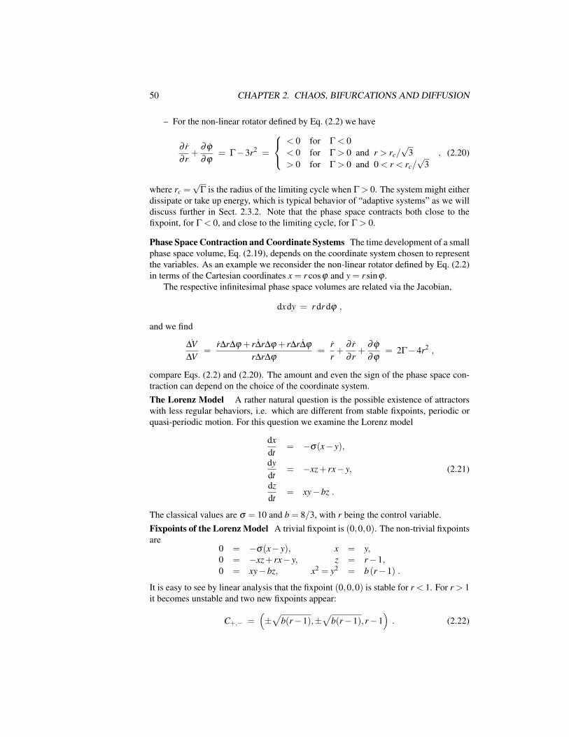
50 CHAPTER 2. CHAOS, BIFURCATIONS AND DIFFUSION
– For the non-linear rotator defined by Eq. (2.2) we have
∂ r∂ r
+∂ ϕ
∂ϕ= Γ−3r2 =
< 0 for Γ< 0< 0 for Γ> 0 and r > rc/
√3
> 0 for Γ> 0 and 0< r < rc/√
3, (2.20)
where rc =√
Γ is the radius of the limiting cycle when Γ> 0. The system might eitherdissipate or take up energy, which is typical behavior of “adaptive systems” as we willdiscuss further in Sect. 2.3.2. Note that the phase space contracts both close to thefixpoint, for Γ< 0, and close to the limiting cycle, for Γ> 0.
Phase Space Contraction and Coordinate Systems The time development of a smallphase space volume, Eq. (2.19), depends on the coordinate system chosen to representthe variables. As an example we reconsider the non-linear rotator defined by Eq. (2.2)in terms of the Cartesian coordinates x = r cosϕ and y = r sinϕ .
The respective infinitesimal phase space volumes are related via the Jacobian,
dxdy = r dr dϕ ,
and we find
∆V∆V
=r∆r∆ϕ + r∆r∆ϕ + r∆r∆ϕ
r∆r∆ϕ=
rr+
∂ r∂ r
+∂ ϕ
∂ϕ= 2Γ−4r2 ,
compare Eqs. (2.2) and (2.20). The amount and even the sign of the phase space con-traction can depend on the choice of the coordinate system.The Lorenz Model A rather natural question is the possible existence of attractorswith less regular behaviors, i.e. which are different from stable fixpoints, periodic orquasi-periodic motion. For this question we examine the Lorenz model
dxdt
= −σ(x− y),
dydt
= −xz+ rx− y, (2.21)
dzdt
= xy−bz .
The classical values are σ = 10 and b = 8/3, with r being the control variable.Fixpoints of the Lorenz Model A trivial fixpoint is (0,0,0). The non-trivial fixpointsare
0 = −σ(x− y), x = y,0 = −xz+ rx− y, z = r−1,0 = xy−bz, x2 = y2 = b(r−1) .
It is easy to see by linear analysis that the fixpoint (0,0,0) is stable for r < 1. For r > 1it becomes unstable and two new fixpoints appear:
C+,− =(±√
b(r−1),±√
b(r−1),r−1). (2.22)

2.3. DISSIPATION AND ADAPTION 51
Figure 2.8: The Sierpinski carpet and its iterative construction
These are stable for r < rc = 24.74 (σ = 10 and b = 8/3). For r > rc the behaviorbecomes more complicated and generally non-periodic.
Strange Attractors One can show, that the Lorenz model has positive Lyapunovexponents for r > rc. It is chaotic with sensitive dependence on the initial conditions.The Lorenz model is at the same time dissipative, since
∂ x∂x
+∂ y∂y
+∂ z∂ z
= −(σ +1+b) < 0, σ > 0, b> 0 . (2.23)
The attractor of the Lorenz system therefore cannot be a smooth surface. Close to theattractor the phase space contracts. At the same time two nearby orbits are repelled dueto the positive Lyapunov exponents. One finds a self-similar structure for the Lorenzattractor with a fractal dimension 2.06 ± 0.01. Such a structure is called a strangeattractor.
The Lorenz model has an important historical relevance in the development ofchaos theory and is now considered a paradigmatic example of a chaotic system.
Fractals Self-similar structures are called fractals. Fractals can be defined by recurrentgeometric rules; examples are the Sierpinski triangle and carpet (see Fig. 2.8) and theCantor set. Strange attractors are normally multifractals, i.e. fractals with non-uniformself-similarity.
The Hausdorff Dimension An important notion in the theory of fractals is the“Hausdorff dimension”. We consider a geometric structure defined by a set of pointsin d dimensions and the number N(l) of d-dimensional spheres of diameter l needed tocover this set. If N(l) scales like
N(l) ∝ l−DH , for l → 0 , (2.24)
then DH is called the Hausdorff dimension of the set. Alternatively we can rewriteEq. (2.24) as
N(l)N(l′)
=
(ll′
)−DH
, DH = − log[N(l)/N(l′)]log[l/l′]
, (2.25)
which is useful for self-similar structures (fractals).

52 CHAPTER 2. CHAOS, BIFURCATIONS AND DIFFUSION
The d-dimensional spheres necessary to cover a given geometrical structure willgenerally overlap. The overlap does not affect the value of the fractal dimension as longas the degree of overlap does not change qualitatively with decreasingdiameter l.The Hausdorff Dimension of the Sierpinski Carpet For the Sierpinski carpet weincrease the number of points N(l) by a factor of 8, compare Fig. 2.9, when we decreasethe length scale l by a factor of 3 (see Fig. 2.8):
DH → −log[8/1]log[1/3]
=log8log3
≈ 1.8928.
2.3.2 Adaptive Systems
Adaptive Systems A general complex system is neither fully conserving nor fullydissipative. Adaptive systems will have periods where they take up energy and periodswhere they give energy back to the environment. An example is the non-linear rotatorof Eq. (2.2), see also Eq. (2.20).
In general one affiliates with the term “adaptive system” the notion of complexityand adaption. Strictly speaking any dynamical system is adaptive if ∇ · x may takeboth positive and negative values. In practice, however, it is usual to reserve the termadaptive system to dynamical systems showing a certain complexity, such as emergingbehavior.The Van der Pol Oscillator Circuits or mechanisms built for the purpose of con-trolling an engine or machine are intrinsically adaptive. An example is the van der Poloscillator,
x − ε(1− x2)x + x = 0,x = yy = ε(1− x2)y− x
(2.26)
where ε > 0 and where we have used the phase space variables x = (x,y). We evaluatethe time evolution ~∇ · x of the phasespace volume,
~∇ · x = +ε(1− x2) .
The oscillator takes up/dissipates energy for x2 < 1 and x2 > 1, respectively. A simplemechanical example for a system with similar properties is illustrated inFig. 2.9Secular Perturbation Theory We consider a perturbation expansion in ε. The solu-tion of Eq. (2.26) is
x0(t) = aei(ω0t+φ) + c.c., ω0 = 1 , (2.27)
for ε = 0. We note that the amplitude a and phase φ are arbitrary in Eq. (2.27). Theperturbation ε(1− x2)x might change, in principle, also the given frequency ω0 = 1 byan amount ∝ ε. In order to account for this “secular perturbation” we make the ansatz
x(t) =[A(T )eit +A∗(T )e−it] + εx1 + · · · , A(T ) = A(εt) , (2.28)
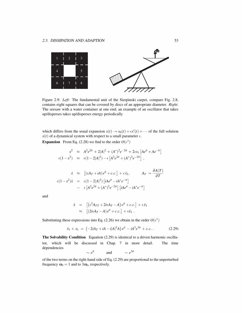
2.3. DISSIPATION AND ADAPTION 53
31
4
6
2
5
7 8
Figure 2.9: Left: The fundamental unit of the Sierpinski carpet, compare Fig. 2.8,contains eight squares that can be covered by discs of an appropriate diameter. Right:The seesaw with a water container at one end; an example of an oscillator that takesup/disperses takes up/disperses energy periodically
which differs from the usual expansion x(t)→ x0(t)+ εx′(t)+ · · · of the full solutionx(t) of a dynamical system with respect to a small parameter ε.Expansion From Eq. (2.28) we find to the order O(ε1)
x2 ≈ A2e2it + 2|A|2 + (A∗)2e−2it + 2εx1[Aeit +Ae−it]
ε(1− x2) ≈ ε(1−2|A|2)− ε[A2e2it +(A∗)2e−2it] ,
x ≈[(εAT + iA)eit + c.c.
]+ ε x1, AT =
∂A(T )∂T
ε(1− x2)x = ε(1−2|A|2)[iAeit − iA∗e−it]
− ε[A2e2it +(A∗)2e−2it][iAeit − iA∗e−it]
and
x =[(ε2AT T +2iεAT −A
)eit + c.c.
]+ ε x1
≈[(2iεAT −A)eit + c.c.
]+ εx1 .
Substituting these expressions into Eq. (2.26) we obtain in the order O(ε1)
x1 + x1 =(−2iAT + iA− i|A|2A
)eit − iA3e3it + c.c. . (2.29)
The Solvability Condition Equation (2.29) is identical to a driven harmonic oscilla-tor, which will be discussed in Chap. 7 in more detail. The timedependencies
∼ eit and ∼ e3it
of the two terms on the right-hand side of Eq. (2.29) are proportional to the unperturbedfrequency ω0 = 1 and to 3ω0, respectively.

54 CHAPTER 2. CHAOS, BIFURCATIONS AND DIFFUSION
–4
–2
0
2
4x(t)
Figure 2.10: The solution of the van der Pol oscillator, Eq. (2.26), for small ε and twodifferent initial conditions. Note the self-generated amplitude stabilization
The term ∼ eit is therefore exactly at resonance and would induce a diverging re-sponse x1→ ∞, in contradiction to the perturbative assumption made by ansatz (2.28).Its prefactor must therefore vanish:
AT =∂A∂T
=12(1−|A|2
)A,
∂A∂ t
=ε
2(1−|A|2
)A , (2.30)
where we have used T = εt. The solubility condition Eq. (2.30) can be written as
a eiφ + iφ aeiφ =ε
2(1−a2)aeiφ
in phase-magnitude representation A(t) = a(t)eiφ(t), or
a = ε(1−a2
)a/2,
φ ∼ O(ε2) .(2.31)
The system takes up energy for a < 1 and the amplitude a increases until the satura-tion limit a→ 1, the conserving point. For a > 1 the system dissipates energy to theenvironment and the amplitude a decreases, approaching unity for t → ∞, just as wediscussed in connection with Eq. (2.2).
The solution x(t) ≈ 2acos(t), compare Eqs. (2.28) and (2.31), of the van derPol equations therefore constitutes an amplitude-regulated oscillation, as illustratedin Fig. 2.10. This behavior was the technical reason for historical development of thecontrol systems that are described by the van der Pol equation (2.26).Lienard Variables For large ε it is convenient to define, compare Eq. (2.26), with
εddt
Y (t) = x(t) − ε(1− x2(t)
)x(t) = −x(t) (2.32)
orεY = X − ε
(1−X2) X , X(t) = x(t),

2.3. DISSIPATION AND ADAPTION 55
X
Y
–a0
a0
21
1
2
x
y
1
–a0
a0
1
2
2
Figure 2.11: Van der Pol oscillator for a large driving c ≡ ε. Left: The relaxationoscillations with respect to the Lienard variables Eq. (2.33). The arrows indicate theflow (X ,Y ), for c = 3, see Eq. (2.33). Also shown is the X = 0 isocline Y =−X +X3/3(solid line) and the limiting cycle, which includes the dashed line with an arrow andpart of the isocline. Right: The limiting cycle in terms of the original variables (x,y) =(x, x) = (x,v). Note that X(t) = x(t)
the Lienard variables X(t) and Y (t). Integration of Y with respect to t yields
εY = X − ε(
X− X3
3
),
where we have set the integration constant to zero. We obtain, together with Eq. (2.32),
X = c(
Y − f (X))
Y = −X/cf (X) = X3/3−X , (2.33)
where we have set c≡ ε, as we are now interested in the case c 1.Relaxation Oscillations We discuss the solution of the van der Pol oscillator Eq. (2.33)for a large driving c graphically, compare Fig. 2.11, by considering the flow (X ,Y ) inphase space (X ,Y ). For c 1 there is a separation of timescales,
(X ,Y ) ∼ (c,1/c), X Y ,
which leads to the following dynamical behavior:
– Starting at a general (X(t0),Y (t0)) the orbit develops very fast ∼ c and nearlyhorizontally until it hits the “isocline”1
X = 0, Y = f (X) = −X +X3/3 . (2.34)
– Once the orbit is close to the X = 0 isocline Y = −X +X3/3 the motion slowsdown and it develops slowly, with a velocity ∼ 1/c close-to (but not exactly on)the isocline (Eq. (2.34)).
1The term isocline stands for “equal slope” in ancient Greek.

56 CHAPTER 2. CHAOS, BIFURCATIONS AND DIFFUSION
– Once the slow motion reaches one of the two local extrema X = ±a0 = ±1 ofthe isocline, it cannot follow the isocline any more and makes a rapid transi-tion towards the other branch of the X = 0 isocline, with Y ≈ const. Note, thattrajectories may cross the isocline vertically, e.g. right at the extrema Y |X=±1 =∓1/c is small but finite.
The orbit therefore relaxes rapidly towards a limiting oscillatory trajectory, illus-trated in Fig. 2.11, with the time needed to perform a whole oscillation depending onthe relaxation constant c; therefore the term “relaxation oscillation”. Relaxation os-cillators represent an important class of cyclic attractors, allowing to model systemsgoing through several distinct and well characterized phases during the course of onecycle. We will discuss relaxation oscillators further in Chap. 7.
2.4 Diffusion and Transport
Deterministic vs. Stochastic Time Evolution So far we have discussed some con-cepts and examples of deterministic dynamical systems, governed by sets of coupleddifferential equations without noise or randomness. At the other extreme are diffusionprocesses for which the random process dominates the dynamics.
Dissemination of information through social networks is one of many exampleswhere diffusion processes plays a paramount role. The simplest model of diffusionis the Brownian motion, which is the erratic movement of grains suspended in liquidobserved by the botanist Robert Brown as early as 1827. Brownian motion became theprototypical example of a stochastic process after the seminal works of Einstein andLangevin at the beginning of the 20th century.
2.4.1 Random Walks, Diffusion and Levy Flights
One-Dimensional Diffusion We consider the random walk of a particle along a line,with the equal probability 1/2 to move left/right at every time step. The probability
pt(x), x = 0,±1,±2, . . . , t = 0,1,2, . . .
to find the particle at time t at position x obeys the master equation
pt+1(x) =12
pt(x−1) +12
pt(x+1) . (2.35)
In order to obtain the limit of continuous time and space, we introduce explicitly thesteps ∆x and ∆t in space and time, and write
pt+∆t(x)− pt(x)∆t
=(∆x)2
2∆tpt(x+∆x)+ pt(x−∆x)−2pt(x)
(∆x)2 . (2.36)

2.4. DIFFUSION AND TRANSPORT 57
Figure 2.12: Examples of random walkers with scale-free distributions ∼ |∆x|1+β forthe real-space jumps, see Eq. (2.40). Left: β = 3, which falls into the universalityclass of standard Brownian motion. Right: β = 0.5, a typical Levy flight. Note theoccurrence of longer-ranged jumps in conjunction with local walking
Now, taking the limit ∆x,∆t → 0 in such a way that (∆x)2/(2∆t) remains finite, weobtain the diffusion equation
∂ p(x, t)∂ t
= D∂ 2 p(x, t)
∂x2 D =(∆x)2
2∆t. (2.37)
Solution of the Diffusion Equation The solution to Eq. (2.37) is readily obtained as2
p(x, t) =1√
4πDtexp(− x2
4Dt
),
∫∞
−∞
dxρ(x, t) = 1 , (2.38)
for the initial condition ρ(x, t = 0) = δ (x). From Eq. (2.38) one concludes that thevariance of the displacement follows diffusive behavior, i.e.
〈x2(t)〉 = 2Dt , x =√〈x2(t)〉 =
√2Dt . (2.39)
Diffusive transport is characterized by transport sublinear in time in contrast toballistic transport with x = vt, as illustrated in Fig. 2.12.Levy Flights We can generalize the concept of a random walker, which is at the basisof ordinary diffusion, and consider a random walk with distributions p(∆t) and p(∆x)for waiting times ∆ti and jumps ∆xi, at every step i = 1, 2, . . . of the walk, as illustratedin Fig. 2.13. One may assume scale-free distributions
p(∆t) ∼ 1(∆t)1+α
, p(∆x) ∼ 1(∆x)1+β
, α,β > 0 . (2.40)
If α > 1 (finite mean waiting time) and β > 2 (finite variance), nothing special hap-pens. In this case the central limiting theorem for well behaved distribution functions
2Note:∫
e−x2/adx =√
aπ and lima→0 exp(−x2/a)/√
aπ = δ (x).

58 CHAPTER 2. CHAOS, BIFURCATIONS AND DIFFUSION
∆ti
∆xi
dis
tan
ce
time
Figure 2.13: A random walker with distributed waiting times ∆ti and jumps ∆xi maybecome a generalized Levy flight
is valid for the spatial component and one obtains standard Brownian diffusion. Re-laxing the above conditions one finds four regimes: normal Brownian diffusion, “Levyflights”, fractional Brownian motion, also denoted “subdiffusion” and generalized Levyflights termed “ambivalent processes”. Their respective scaling laws are listed in Table2.1 and two examples are shown in Fig. 2.12.
Levy flights occur in a wide range of processes, such as in the flight patterns ofwandering albatrosses or in human travel habits, which seem to be characterized by ageneralized Levy flight with α,β ≈ 0.6.
Diffusion Within Networks Diffusion occurs in many circumstances. We considerhere the case of diffusion within a network, such as the diffusion of information withinsocial networks. This is an interesting issue as the control of information is importantfor achieving social influence and prestige. We will however neglect in the followingthe creation of new information, which is clearly relevant for real-life applications.
Consider a network of i = 1, . . . ,N vertices connected by edges with weight Wi j,corresponding to the elements of the weighted adjacency matrix. We denote by
ρi(t),N
∑i=1
ρi(t) = 1
the density of information present at time t and vertex i.
Flow of Information The information flow can then be described by the masterequation
ρi(t +∆t) = ρi(t) + J(+)i (t)∆t − J(−)i (t)∆t , (2.41)
where J(±)i (t) denotes the density of information entering (+) and leaving (−) vertex i
Table 2.1: The four regimes of a generalized walker with distribution functions,Eq. (2.40), characterized by scalings ∝ (∆t)−1−α and ∝ (∆x)−1−β for the waiting times∆t and jumps ∆x, as depicted in Fig. 2.13
α > 1 β > 2 x∼√
t Ordinary diffusionα > 1 0< β < 2 x∼ t1/β Levy flights0< α < 1 β > 2 x∼ tα/2 Subdiffusion0< α < 1 0< β < 2 x∼ tα/β Ambivalent processes

2.4. DIFFUSION AND TRANSPORT 59
per time interval ∆t, given by
J(+)i (t) = ∑
j
Wi j
∑k Wk jρ j(t), J(−)i (t) = ∑
j
Wji
∑k Wkiρi(t) = ρi(t) .
Introducing the time step ∆t = 1 and the expressions for J(±)i (t) into Eq. (2.41) we find
ρi(t +∆t)−ρi(t)∆t
=∂
∂ tρi(t) = ∑
jTi j ρ j(t) − ρi(t) , (2.42)
where we have performed the limit ∆t→ 0 and defined
Ti j =Wi j
∑k Wk j.
This equation can easily be cast into the following matrix form:
∂
∂ t~ρ(t) = D~ρ(t), Di j = Ti j−δi j , (2.43)
where ~ρ = (ρ1, . . . ,ρN). It resembles the diffusion equation (2.36), so we may denoteD = (Di j) as the diffusion matrix (or operator). Physically, Eq. (2.42) means thatT = (Ti j) transfers (propagates) the energy density ~ρ(t) one step forward in time. Dueto this property, T has been termed the “transfer matrix”.
The Stationary State When no new information is created we may expect the distri-bution of information to settle into a stationary state
∂ρi(t)∂ t
→ 0, ρi(t) → ρi(∞) .
Formally, the stationary state corresponds to the unitary eigenvalue of T, see Eq. (2.42).Here we assume
ρi(∞) ∝ ∑j
Wji , (2.44)
in Eq. (2.42):
∑j
Wi j
∑k Wk j∑k
Wk j = ∑l
Wli, ∑j
Wi j = ∑l
Wli . (2.45)
Consequently, a global steady state has the form of the ansatz (2.44) when the weightof incoming links ∑ j Wi j equals the weight of outgoing links ∑l Wli for every vertexi. That is if there are no sinks or sources for information. The condition Eq. (2.45)is fulfilled for symmetric weight matrices with Wi j = Wji. The information density isproportional to the vertex degree, ρi(∞) ∝ ki, when the Wi j reduces to the adjacencymatrix.

60 CHAPTER 2. CHAOS, BIFURCATIONS AND DIFFUSION
2.4.2 The Langevin Equation and Diffusion
Diffusion as a Stochastic Process Langevin proposed to describe the diffusion of aparticle by the stochastic differential equation
mv = −mγ v + ξ (t), < ξ (t)>= 0, < ξ (t)ξ (t ′)>= Qδ (t− t ′), (2.46)
where v(t) is the velocity of the particle and m> 0 its mass.
(i) The term−mγv on the right-hand-side of Eq. (2.46) corresponds to a damping term,the friction being proportional to γ > 0.
(ii) ξ (t) is a stochastic variable, viz noise. The brackets < .. . > denote ensembleaverages, i.e. averages over different noise realizations.
(iii) As white noise (in contrast to colored noise) one denotes noise with a flat powerspectrum (as white light), viz < ξ (t)ξ (t ′)>∝ δ (t− t ′).
(iv) The constant Q is a measure for the strength of the noise.
Solution of the Langevin Equation Considering a specific noise realization ξ (t),one finds
v(t) = v0 e−γt +e−γt
m
∫ t
0dt ′ eγt ′
ξ (t ′) (2.47)
for the solution of the Langevin Eq. (2.46), where v0 ≡ v(0).
Mean Velocity For the ensemble average < v(t)> of the velocity one finds
< v(t)> = v0 e−γt +e−γt
m
∫ t
0dt ′ eγt ′ < ξ (t ′)>︸ ︷︷ ︸
0
= v0 e−γt . (2.48)
The average velocity decays exponentially to zero.
Mean Square Velocity For the ensemble average < v2(t) > of the velocity squaredone finds
< v2(t)> = v20 e−2γt +
2v0 e−2γt
m
∫ t
0dt ′ eγt ′ < ξ (t ′)>︸ ︷︷ ︸
0
+e−2γt
m2
∫ t
0dt ′∫ t
0dt ′′ eγt ′ eγt ′′ < ξ (t ′)ξ (t ′′)>︸ ︷︷ ︸
Qδ (t ′−t ′′)
= v20 e−2γt +
Qe−2γt
m2
∫ t
0dt ′ e2γt ′︸ ︷︷ ︸
(e2γt−1)/(2γ)
2.5. NOISE-CONTROLLED DYNAMICS 61
and finally
< v2(t)> = v20 e−2γt +
Q2γ m2
(1− e−2γt) . (2.49)
For long times the average squared velocity
limt→∞
< v2(t)> =Q
2γ m2 (2.50)
becomes, as expected, independent of the initial velocity v0. Equation (2.50) showsexplicitly that the dynamics is driven exclusively by the stochastic process ∝ Q forlong time scales.The Langevin Equation and Diffusion The Langevin equation is formulated in termsof the particle velocity. In order to make connection with the time evolution of a real-space random walker, Eq. (2.39), we multiply the Langevin equation (2.46) by x andtake the ensemble average:
< x v> = −γ < xv> +1m< xξ > . (2.51)
We note that
xv = x x =ddt
x2
2, x v = x x =
d2
dt2x2
2− x2, < xξ >= x< ξ >= 0 .
We then find for Eq. (2.51)
d2
dt2< x2 >
2−< v2 > = −γ
ddt< x2 >
2or
d2
dt2 < x2 > +γddt< x2 > = 2< v2 > =
Qγm2 , (2.52)
where we have used the long-time result Eq. (2.50) for < v2 >. The solution ofEq. (2.52) is
< x2 > =[γt−1+ e−γt] Q
γ3m2 . (2.53)
For long times we find
limt→∞
< x2 > =Q
γ2m2 t ≡ 2Dt, D =Q
2γ2m2 (2.54)
diffusive behavior, compare Eq. (2.39). This shows that diffusion is microscopicallydue to a stochastic process, since D ∝ Q.
2.5 Noise-Controlled Dynamics
Stochastic Systems A set of first-order differential equations with a stochastic termis generally denoted a “stochastic system”. The Langevin equation (2.46) discussed inSect. 2.4.2 is a prominent example. The stochastic term corresponds quite generally tonoise. Depending on the circumstances, noise might be very important for the long-term dynamical behavior. Some examples of this are as follows:

62 CHAPTER 2. CHAOS, BIFURCATIONS AND DIFFUSION
– Neural Networks: Networks of interacting neurons are responsible for the cog-nitive information processing in the brain. They must remain functional also inthe presence of noise and need to be stable as stochastic systems. In this casethe introduction of a noise term to the evolution equation should not change thedynamics qualitatively. This postulate should be valid for the vast majorities ofbiological networks.
– Diffusion: The Langevin equation reduces, in the absence of noise, to a dampedmotion without an external driving force, with v = 0 acting as a global attrac-tor. The stochastic term is therefore essential in the long-time limit, leading todiffusive behavior.
– Stochastic Escape and Stochastic Resonance: A particle trapped in a localminimum may escape this minimum by a noise-induced diffusion process; aphenomenon called “stochastic escape”. Stochastic escape in a driven bistablesystem leads to an even more subtle consequence of noise-induced dynamics,the “stochastic resonance”.
2.5.1 Stochastic Escape
Drift Velocity We generalize the Langevin equation (2.46) and consider an externalpotential V (x),
mv = −mγ v + F(x) + ξ (t), F(x) =−V ′(x) =− ddx
V (x) , (2.55)
where v,m are the velocity and the mass of the particle,< ξ (t)>= 0 and< ξ (t)ξ (t ′)>=Qδ (t− t ′). In the absence of damping (γ = 0) and noise (Q = 0), Eq. (2.55) reduces toNewton’s law.
We consider for a moment a constant force F(x) = F and the absence of noise,ξ (t)≡ 0. The system then reaches an equilibrium for t→∞ when relaxation and forcecancel each other:
mvD = −mγ vD + F ≡ 0, vD =F
γm. (2.56)
vD is called the “drift velocity”. A typical example is the motion of electrons in a metal-lic wire. An applied voltage, which leads an electric field along the wire, induces anelectrical current (Ohm’s law). This results in the drifting electrons being continuouslyaccelerated by the electrical field, while bumping into lattice imperfections or collidingwith the lattice vibrations, i.e. the phonons.
The Fokker–Planck Equation We consider now an ensemble of particles diffusingin an external potential, and denote with P(x, t) the density of particles at location xand time t. Particle number conservation defines the particle current density J(x, t) viathe continuity equation
∂P(x, t)∂ t
+∂J(x, t)
∂x= 0. (2.57)

2.5. NOISE-CONTROLLED DYNAMICS 63
There are two contributions, JvD and Jξ , to the total particle current density, J = JvD +Jξ , induced by the diffusion and by the stochastic motion respectively. We derive thesetwo contributions in two steps.
In a first step we consider with Q = 0 the absence of noise in Eq. (2.55). Theparticles then move uniformly with the drift velocity vD in the stationary limit, and thecurrent density is
JvD = vD P(x, t) .
In a second step we set the force to zero, F = 0, and derive the contribution Jξ ofthe noise term ∼ ξ (t) to the particle current density. For this purpose we rewrite thediffusion equation (2.37)
∂P(x, t)∂ t
= D∂ 2P(x, t)
∂x2 ≡ −∂Jξ (x, t)
∂x∂P(x, t)
∂ t+
∂Jξ (x, t)∂x
= 0
as a continuity equation, which allows us to determine the functional form of Jξ ,
Jξ = −D∂P(x, t)
∂x. (2.58)
Using the relation D = Q/(2γ2m2), see Eq. (2.54), and including the drift term we find
J(x, t) = vD P(x, t) − D∂P(x, t)
∂x=
Fγm
P(x, t) − Q2γ2m2
∂P(x, t)∂x
(2.59)
for the total current density J = JvD + Jξ . Using expression (2.59) for the total particlecurrent density in (2.57) one obtains the “Fokker–Planck” or “Smoluchowski” equation
∂P(x, t)∂ t
= −∂vD P(x, t)∂x
+∂ 2DP(x, t)
∂x2 (2.60)
for the density distribution P(x, t).The Harmonic Potential
We consider the harmonic confining potential
V (x) =f2
x2, F(x) = − f x ,
and a stationary density distribution,
dP(x, t)dt
= 0 =⇒ dJ(x, t)dx
= 0 .
Expression (2.59) yields then the differential equation
ddx
[f xγ m
+Q
2γ2m2ddx
]P(x) = 0 =
ddx
[β f x+
ddx
]P(x),
with β = 2γm/Q and where for the stationary distribution function P(x) =limt→∞ P(x, t). The system is confined and the steady-state current vanishes conse-quently. We find
P(x) = Ae−βf2 x2
= Ae−βV (x) A =
√f γmπQ
, (2.61)

64 CHAPTER 2. CHAOS, BIFURCATIONS AND DIFFUSION
V(x)
P(x)∆V
J
xmax xmin
Figure 2.14: Left: Stationary distribution P(x) of diffusing particles in a harmonicpotential V (x). Right: Stochastic escape from a local minimum, with ∆V =V (xmax)−V (xmin) being the potential barrier height and J the escape current
where the prefactor is determined by the normalization condition∫
dxP(x) = 1. Thedensity of diffusing particles in a harmonic trap is Gaussian-distributed, see Fig. 2.14.
The Escape Current We now consider particles in a local minimum, as depicted inFig. 2.14, with a typical potential having a functional form like
V (x) ∼ −x + x3 . (2.62)
Without noise, the particle will oscillate around the local minimum eventually comingto a standstill x→ xmin under the influence of friction.
With noise, the particle will have a small but finite probability
∝ e−β∆V , ∆V =V (xmax)−V (xmin)
to reach the next saddlepoint, where ∆V is the potential difference between the saddle-point and the local minimum, see Fig. 2.14. The solution Eq. (2.61) for the stationaryparticle distribution in a confining potential V (x) has a vanishing total current J. Fornon-confining potentials, like Eq. (2.62), the particle current J(x, t) never vanishes.Stochastic escape occurs when starting with a density of diffusing particles close thelocal minimum, as illustrated in Fig. 2.14. The escape current will be nearly constantwhenever the escape probability is small. In this case the escape current will be pro-portional to the probability a particle has to reach the saddlepoint,
J(x, t)∣∣∣x=xmax
∝ e−β [V (xmax)−V (xmin)] ,
when approximating the functional dependence of P(x) with that valid for the harmonicpotential, Eq. (2.61).
Kramer’s Escape When the escape current is finite, there is a finite probability perunit of time for the particle to escape the local minima, the Kramer’s escape rate rK ,
rK =ωmaxωmin
2π γexp [−β (V (xmax)−V (xmin))] , (2.63)

2.5. NOISE-CONTROLLED DYNAMICS 65
V(x,t)
Figure 2.15: The driven double-well potential, V (x)−A0 cos(Ωt)x, compare Eq. (2.64).The driving force is small enough to retain the two local minima
where the prefactors ωmin =√|V ′′(xmin)|/m and ωmax =
√|V ′′(xmax)|/m can be de-
rived from a more detailed calculation, and where β = 2γm/Q.Stochastic Escape in Evolution Stochastic escape occurs in many real-world sys-tems. Noise allows the system to escape from a local minimum where it would other-wise remain stuck for eternity.
As an example, we mention stochastic escape from a local fitness maximum (inevolution fitness is to be maximized) by random mutations that play the role of noise.These issues will be discussed in more detail in Chap. 6.
2.5.2 Stochastic Resonance
The Driven Double-Well Potential We consider diffusive dynamics in a drivendouble-well potential, see Fig. 2.15,
x = −V ′(x)+A0 cos(Ωt)+ξ (t), V (x) =−12
x2 +14
x4 . (2.64)
The following is to be remarked:
– Equation (2.64) corresponds to the Langevin equation (2.55) in the limit of verylarge damping, γ m, keeping γm≡ 1 constant (in dimensionless units).
– The potential in Eq. (2.64) is in normal form, which one can always achieve byrescaling the variables appropriately.
– The potential V (x) has two minima x0 at
−V ′(x) = 0 = x− x3 = x(1− x2), x0 =±1 .
The local maximum x0 = 0 is unstable.
– We assume that the periodic driving ∝ A0 is small enough, such that the effectivepotential V (x)−A0 cos(Ωt)x retains two minima at all times, compare Fig. 2.15.
Transient State Dynamics The system will stay close to one of the two minima, x≈±1, for most of the time when both A0 and the noise strength are weak, see Fig. 2.16.This is an instance of “transient state dynamics”, which will be discussed in more detailin Chap. 8. The system switches between a set of preferred states.Switching Times An important question is then: How often does the system switchbetween the two preferred states x≈ 1 and x≈−1? There are two time scales present:

66 CHAPTER 2. CHAOS, BIFURCATIONS AND DIFFUSION
– In the absence of external driving, A0 ≡ 0, the transitions are noise driven andirregular, with the average switching time given by Kramer’s lifetime TK = 1/rK ,see Fig. 2.16. The system is translational invariant with respect to time and theensemble averaged expectation value
< x(t)> = 0
therefore vanishes in the absence of an external force.
– When A0 6= 0 the external force induces a reference time and a non-zero responsex,
< x(t)> = x cos(Ωt− φ) , (2.65)
which follows the time evolution of the driving potential with a certain phaseshift φ , see Fig. 2.17.
The Resonance Condition When the time scale 2TK = 2/rK to switch back and forthdue to the stochastic process equals the period 2π/Ω, we expect a large response x, seeFig. 2.17. The time-scale matching condition
2π
Ω≈ 2
rK
depends on the noise-level Q, via Eq. (2.63), for the Kramer’s escape rate rK . Theresponse x first increases with rising Q and then becomes smaller again, for otherwiseconstant parameters, see Fig. 2.17. Therefore the name “stochastic resonance”.Stochastic Resonance and the Ice Ages The average temperature Te of the earthdiffers by about ∆Te ≈ 10C in between a typical ice age and the interglacial periods.Both states of the climate are locally stable.
– The Ice Age: The large ice covering increases the albedo of the earth and a largerpart of sunlight is reflected back to space. The earth remains cool.
– The Interglacial Period: The ice covering is small and a larger portion of thesunlight is absorbed by the oceans and land. The earth remains warm.
A parameter of the orbit of the planet earth, the eccentricity, varies slightly with a periodT = 2π/Ω≈ 105 years. The intensity of the incoming radiation from the sun thereforevaries with the same period. Long-term climate changes can therefore be modeled bya driven two-state system, i.e. by Eq. (2.64). The driving force, viz the variation ofthe energy flux the earth receives from the sun, is however very small. The increasein the amount of incident sunlight is too weak to pull the earth out of an ice age intoan interglacial period or vice versa. Random climatic fluctuation, like variations in thestrength of the gulf stream, are needed to finish the job. The alternation of ice ages withinterglacial periods may therefore be modeled as a stochastic resonance phenomenon.Neural Networks and Stochastic Resonance Neurons are driven bistable devicesoperating in a noisy environment. It is therefore not surprising that stochastic resonancemay play a role for certain neural network setups with undercritical driving.Beyond Stochastic Resonance Resonance phenomena generally occur when twofrequencies, or two time scales, match as a function of some control parameter. Forthe case of stochastic resonance these two time scales correspond to the period of the
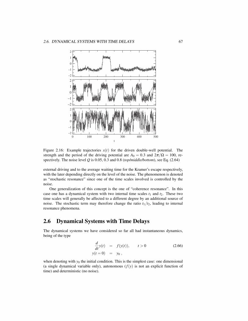
2.6. DYNAMICAL SYSTEMS WITH TIME DELAYS 67
–2
–1
0
1
2
–2
–1
0
1
2
0 100 200 300 400 500
t
–2
–1
0
1
2
Figure 2.16: Example trajectories x(t) for the driven double-well potential. Thestrength and the period of the driving potential are A0 = 0.3 and 2π/Ω = 100, re-spectively. The noise level Q is 0.05, 0.3 and 0.8 (top/middle/bottom), see Eq. (2.64)
external driving and to the average waiting time for the Kramer’s escape respectively,with the later depending directly on the level of the noise. The phenomenon is denotedas “stochastic resonance” since one of the time scales involved is controlled by thenoise.
One generalization of this concept is the one of “coherence resonance”. In thiscase one has a dynamical system with two internal time scales t1 and t2. These twotime scales will generally be affected to a different degree by an additional source ofnoise. The stochastic term may therefore change the ratio t1/t2, leading to internalresonance phenomena.
2.6 Dynamical Systems with Time DelaysThe dynamical systems we have considered so far all had instantaneous dynamics,being of the type
ddt
y(t) = f (y(t)), t > 0 (2.66)
y(t = 0) = y0 ,
when denoting with y0 the initial condition. This is the simplest case: one dimensional(a single dynamical variable only), autonomous ( f (y) is not an explicit function oftime) and deterministic (no noise).

68 CHAPTER 2. CHAOS, BIFURCATIONS AND DIFFUSION
0 0.2 0.4 0.6 0.8 1
Q
0
0.4
0.8
1.2
x
Figure 2.17: The gain x, see Eq. (2.65), as a function of noise level Q. The strength ofthe driving amplitude A0 is 0.1, 0.2 and 0.3 (bottom/middle/top curves), see Eq. (2.64)and the period 2π/Ω = 100. The response x is very small for vanishing noise Q = 0,when the system performs only small-amplitude oscillations in one of the local minima
Time Delays In many real-world applications the couplings between different sub-systems and dynamical variables is not instantaneous. Signals and physical interactionsneed a certain time to travel from one subsystem to the next. Time delays are thereforeencountered commonly and become important when the delay time T becomes com-parable with the intrinsic time scales of the dynamical system. We consider here thesimplest case, a noise-free one-dimensional dynamical system with a single delay time,
ddt
y(t) = f (y(t),y(t−T )), t > 0 (2.67)
y(t) = φ(t), t ∈ [−T,0] .
Due to the delayed coupling we need now to specify an entire initial function φ(t).Differential equations containing one or more time delays need to be considered verycarefully, with the time delay introducing an additional dimension to the problem. Wewill discuss here a few illustrative examples.Linear Couplings We start with the linear differential equation
ddt
y(t) = −ay(t) − by(t−T ), a,b> 0 . (2.68)
The only constant solution for a+b 6= 0 is the trivial state y(t)≡ 0. The trivial solutionis stable in the absence of time delays, T = 0, whenever a+ b > 0. The question isnow, whether a finite T may change this.
We may expect the existence of a certain critical Tc, such that y(t) ≡ 0 remainsstable for small time delays 0≤ T < Tc. In this case the initial function φ(t) will affectthe orbit only transiently, in the long run the motion would be damped out, approachingthe trivial state asymptotically for t→ ∞.

2.6. DYNAMICAL SYSTEMS WITH TIME DELAYS 69
–3
–2
–1
0
0 0.5 1 1.5 2 2.5 3
delay time T
Im - part q
Re - part p
Figure 2.18: The solution e(p+iq)t of the time-delayed system, Eq. (2.68), for a = 0.1and b = 1. The state y(t)≡ 0 become unstable whenever p> 0. q is given in units of π
Hopf Bifurcation Trying our luck with the usual exponential ansatz, we find
λ = −a−be−λT , y(t) = y0eλ t , λ = p+ iq .
Separating into a real and imaginary part we obtain
p+a = −be−pT cos(qT ),
q = be−pT sin(qT ).(2.69)
For T = 0 the solution is p = −(a+ b), q = 0, as expected, and the trivial solutiony(t) ≡ 0 is stable. A numerical solution is shown in Fig. 2.18 for a = 0.1 and b = 1.The crossing point p = 0 is determined by
a = −bcos(qT ), q = bsin(qT ) . (2.70)
The first condition in Eq. (2.70) can be satisfied only for a < b. Taking the squares inEq. (2.70) and eliminating qT one has
q =√
b2−a2, T ≡ Tc = arccos(−a/b)/q .
One therefore has a Hopf bifurcation at T = Tc and the trivial solution becomesunstable for T > Tc. For the case a = 0 one has simply q = b, Tc = π/(2b). Note, thatthere is a Hopf bifurcation only for a< b, viz whenever the time-delay dominates, andthat q becomes non-zero well before the bifurcation point, compare Fig. 2.18. One hastherefore a region of damped oscillatory behavior with q 6= 0 and p< 0.Discontinuities For time-delayed differential equations one may specify an arbitraryinitial function φ(t) and the solutions may in general show discontinuities in their

70 CHAPTER 2. CHAOS, BIFURCATIONS AND DIFFUSION
derivatives, as a consequence. As an example we consider the case a = 0, b = 1 ofEq. (2.68), with a non-zero constant initial function,
ddt
y(t) = −y(t−T ), φ(t)≡ 1 . (2.71)
The solution can be evaluated simply by stepwise integration,
y(t)− y(0) =∫ t
0dt ′y(t ′) = −
∫ t
0dt ′y(t ′−T ) = −
∫ t
0dt ′ = −t, 0< t < T .
The first derivative in consequently discontinuous at t = 0,
limt→0−
ddt
y(t) = 0, limt→0+
ddt
y(t) = −1 .
For larger times, T < t < 2T , one finds
y(t)− y(T ) =−∫ t
Tdt ′y(t ′−T ) =
∫ t
Tdt ′[t ′−1
]=
t2−T 2
2− (t−T ) ,
and the second derivative has a discontinuity at t = T .
Dependence on Initial Function The solution of ordinary differential equations isdetermined by their initial condition and different initial conditions lead to distincttrajectories (injectivity). This is not necessarily the case anymore in the presence oftime delays. We consider
ddt
y(t) = y(t−T )(y(t)−1
), φ(t = 0) = 1 . (2.72)
For any φ(t) with φ(0) = 1 the solution is y(t)≡ 1 for all t ∈ [0,∞].
Non-Constant Time Delays Thinks may become rather weird when the time delaysare not constant anymore. Consider
ddt y(t) = y
(t−|y(t)|−1
)+ 1
2 , t > 0,
φ(t) =
0 −1< t < 01 t <−1 .
(2.73)
It is easy to see, that both functions
y(t) =t2, y(t) =
3t2, t ∈ [0,2] ,
are solutions of Eq. (2.73), with appropriate continuations for t > 2. Two differentsolutions of the same differential equation and identical initial conditions, that cannothappen for ordinary differential equations. It is evident, that especial care must betaken when examining dynamical systems with time delays numerically.
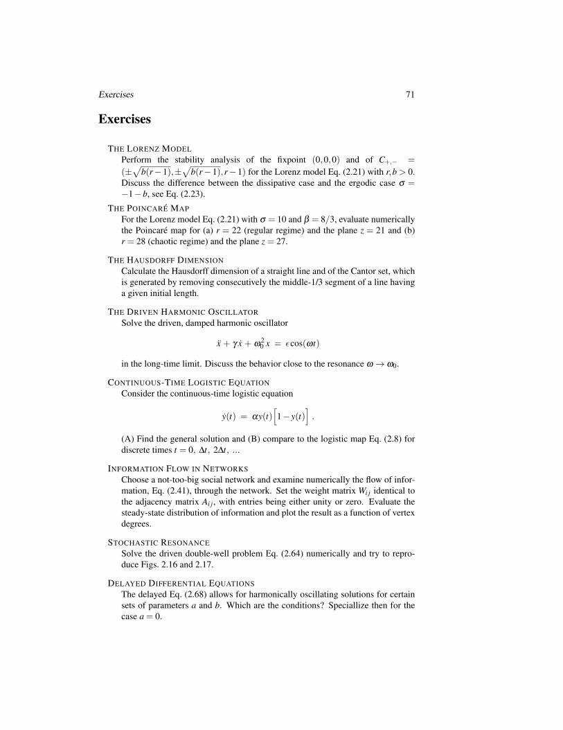
Exercises 71
Exercises
THE LORENZ MODELPerform the stability analysis of the fixpoint (0,0,0) and of C+,− =
(±√
b(r−1),±√
b(r−1),r−1) for the Lorenz model Eq. (2.21) with r,b> 0.Discuss the difference between the dissipative case and the ergodic case σ =−1−b, see Eq. (2.23).
THE POINCARE MAPFor the Lorenz model Eq. (2.21) with σ = 10 and β = 8/3, evaluate numericallythe Poincare map for (a) r = 22 (regular regime) and the plane z = 21 and (b)r = 28 (chaotic regime) and the plane z = 27.
THE HAUSDORFF DIMENSIONCalculate the Hausdorff dimension of a straight line and of the Cantor set, whichis generated by removing consecutively the middle-1/3 segment of a line havinga given initial length.
THE DRIVEN HARMONIC OSCILLATORSolve the driven, damped harmonic oscillator
x + γ x + ω20 x = εcos(ωt)
in the long-time limit. Discuss the behavior close to the resonance ω → ω0.
CONTINUOUS-TIME LOGISTIC EQUATIONConsider the continuous-time logistic equation
y(t) = αy(t)[1− y(t)
].
(A) Find the general solution and (B) compare to the logistic map Eq. (2.8) fordiscrete times t = 0, ∆t, 2∆t, ...
INFORMATION FLOW IN NETWORKSChoose a not-too-big social network and examine numerically the flow of infor-mation, Eq. (2.41), through the network. Set the weight matrix Wi j identical tothe adjacency matrix Ai j, with entries being either unity or zero. Evaluate thesteady-state distribution of information and plot the result as a function of vertexdegrees.
STOCHASTIC RESONANCESolve the driven double-well problem Eq. (2.64) numerically and try to repro-duce Figs. 2.16 and 2.17.
DELAYED DIFFERENTIAL EQUATIONSThe delayed Eq. (2.68) allows for harmonically oscillating solutions for certainsets of parameters a and b. Which are the conditions? Speciallize then for thecase a = 0.

72 2 Chaos, Bifurcations and Diffusion
CAR-FOLLOWING MODELA car moving with velocity x(t) follows another car driving with velocity v(t)via
x(t +T ) = α(v(t)− x(t)), α > 0 , (2.74)
with T > 0 being the reaction time of the driver. Prove the stability of the steady-state solution for a constant velocity v(t)≡ v0 of the preceding car.
Further ReadingFor further studies we refer to introductory texts for dynamical system theory (Katokand Hasselblatt, 1995), classical dynamical systems (Goldstein, 2002), chaos (Schusterand Just, 2005; Devaney, 1989; Gutzwiller, 1990, Strogatz, 1994), stochastic systems(Ross, 1982; Lasota and Mackey, 1994) and differential equations with time delays(Erneux, 2009). Other textbooks on complex and/or adaptive systems are those bySchuster (2001) and Boccara (2003). For an alternative approach to complex systemtheory via Brownian agents consult Schweitzer (2003).
The interested reader may want to study some selected subjects in more depth, suchas the KAM theorem (Ott, 2002), relaxation oscillators (Wang, 1999), stochastic res-onance (Benzit et al., 1981; Gammaitoni et al., 1998), coherence resonance (Pikovskyand Kurths, 1997), Levy flights (Metzler and Klafter, 2000), the connection of Levyflights to the patterns of wandering albatrosses (Viswanathan et al., 1996), human trav-eling (Brockmann, Hufnagel and Geisel, 2006) and diffusion of information in net-works (Eriksen et al., 2003).
The original literature provides more insight, such as the seminal works of Einstein(1905) and Langevin (1908) on Brownian motion or the first formulation and study ofthe Lorenz (1963) model.
BENZIT, R., SUTERA, A., VULPIANI, A. 1981 The mechanism of stochastic resonance.Journal of Physics A 14, L453–L457.
BROCKMANN, D., HUFNAGEL, L., GEISEL, T. 2006 The scaling laws of human travel. Na-ture 439, 462.
BOCCARA, N. 2003 Modeling Complex Systems. Springer, Berlin.
DEVANEY, R.L. 1989 An Introduction to Chaotic Dynamical Systems. Addison-Wesley,Reading, MA.
EINSTEIN, A. 1905 Uber die von der molekularkinetischen Theorie der Warme geforderteBewegung von in ruhenden Flussigkeiten suspendierten Teilchen. Annalen der Physik 17,549.
ERIKSEN, K.A., SIMONSEN, I., MASLOV, S., SNEPPEN, K. 2003 Modularity and extremeedges of the internet. Physical Review Letters 90, 148701.
ERNEUX, T. 2009 Applied Delay Differential Equations. Springer, New York.
GAMMAITONI, L., HANGGI, P., JUNG, P., MARCHESONI, F. 1998 Stochastic resonance.Review of Modern Physics 70, 223–287.
GOLDSTEIN, H. 2002 Classical Mechanics. 3rd Edition, Addison-Wesley, Reading, MA.
GUTZWILLER, M.C. 1990 Chaos in Classical and Quantum Mechanics. Springer, New York.

Further Reading 73
KATOK, A., HASSELBLATT, B. 1995 Introduction to the Modern Theory of Dynamical Sys-tems. Cambridge University Press, Cambridge.
LANGEVIN, P. 1908 Sur la theorie du mouvement brownien. Comptes Rendus 146, 530–532.
LASOTA, A., MACKEY, M.C. 1994 Chaos, Fractals, and Noise – Stochastic Aspects ofDynamics. Springer, New York.
LORENZ, E.N. 1963 Deterministic nonperiodic flow. Journal of the Atmospheric Sciences20, 130–141.
METZLER, R., KLAFTER J. 2000 The random walk’s guide to anomalous diffusion: a frac-tional dynamics approach Physics Reports 339, 1.
OTT, E. 2002 Chaos in Dynamical Systems. Cambridge University Press, Cambridge.
PIKOVSKY, A.S., KURTHS, J. 1997 Coherence resonance in a noise-driven excitable systemPhysical Review Letters 78, 775.
ROSS, S.M. 1982 Stochastic Processes. Wiley, New York.
SCHUSTER, H.G. 2001 Complex Adaptive Systems. Scator, Saarbrucken.
SCHUSTER, H.G., JUST, W. 2005 Deterministic Chaos. 4th. Edition, Wiley-VCH, NewYork.
SCHWEITZER, F. 2003 Brownian Agents and Active Particles: Collective Dynamics in theNatural and Social Sciences. Springer, New York.
STROGATZ, S.H 1994 Nonlinear Systems and Chaos. Perseus Publishing, Cambridge, MA.
VISWANATHAN, G.M., AFANASYEV, V., BULDYREV, S.V., MURPHY, E.J., PRINCE, P.A.,STANLEY, H.E. 1996 Levy flight search patterns of wandering albatrosses. Nature 381,413.
WANG, D.L. 1999 Relaxation oscillators and networks. In J.G. Webster (ed.), Encyclopediaof Electrical and Electronic Engineers, pp. 396–405, Wiley, New York.

74 2 Chaos, Bifurcations and Diffusion

Chapter 3
Complexity and InformationTheory
What do we mean when by saying that a given system shows “complex behavior”,can we provide precise measures for the degree of complexity? This chapter offers anaccount of several common measures of complexity and the relation of complexity topredictability and emergence.
The chapter starts with a self-contained introduction to information theory andstatistics. We will learn about probability distribution functions, the law of large num-bers and the central limiting theorem. We will then discuss the Shannon entropy andthe mutual information, which play central roles both in the context of time series anal-ysis and as starting points for the formulation of quantitative measures of complexity.This chapter then concludes with a short overview over generative approaches to com-plexity.
3.1 Probability Distribution FunctionsStatistics is ubiquitous in everyday life and we are used to chat, e.g., about the probabil-ity that our child will have blue or brown eyes, the chances to win a lottery or those ofa candidate to win the presidential elections. Statistics is also ubiquitous in all realmsof the sciences and basic statistical concepts are used throughout these lecture notes1.Variables and Symbols Probability distribution functions may be defined for contin-uous or discrete variables as well as for sets of symbols,
x ∈ [0,∞], xi ∈ 1,2,3,4,5,6, α ∈ blue,brown,green .
E.g. we may define with p(x) the probability distribution of human life expectancy x,with p(xi) the chances to obtain xi when throwing a dice or with p(α) the probability to
1In some areas, like the neurosciences or artificial intelligence, the term “Bayesian” is used for ap-proaches using statistical methods, in particular in the context of hypothesis building, when estimates ofprobability distribution functions are derived from observations.
75

76 CHAPTER 3. COMPLEXITY AND INFORMATION THEORY
meet somebody having eyes of color α . Probabilities are in any case positive definiteand the respective PDF2 normalized,
p(x), p(xi), p(α) ≥ 0,∫
∞
0p(x)dx = 1 = ∑
α
p(α), . . . .
The notation used for a given variable will indicate in the following its nature, i.e.whether it is a continuous or discrete variable, or denoting a symbol.Continuous vs. Discrete Stochastic Variables When discretizing a stochastic vari-able, e.g. when approximating an integral by a Riemann sum,∫
∞
0p(x)dx ≈
∞
∑i=0
p(xi)∆x, xi = ∆x(0.5+ i) , (3.1)
the resulting discrete PDF p(xi) is not any more normalized; the properly normalizeddiscrete PDF is p(xi)∆x. Note, that both notations pi and p(xi) are used for discretedistribution functions3.Mean, Median and Standard Deviation The average 〈x〉, denoted also by x, andthe standard deviation σ are given by
〈x〉 =∫
x p(x)dx, σ2 =
∫(x− x)2 p(x)dx . (3.2)
One also calls x the expectation value or just the mean, and σ2 the variance4. Foreveryday life situations the median x,∫
x<xp(x)dx =
12
=∫
x>xp(x)dx , (3.3)
is somewhat more intuitive than the mean. We have a 50% chance to meet somebodybeing smaller/taller than the median height.Exponential Distribution Let us consider, as an illustration, the exponential distri-bution, which describes, e.g. the distribution of waiting times for radioactive decay,
p(t) =1T
e−t/T ,∫
∞
0p(t)dt = 1 , (3.4)
with the mean waiting time
〈t〉 = 1T
∫∞
0t e−t/T dt =
tT
e−t/T ∣∣∞0 +
∫∞
0e−t/T dt = T .
The median t and the standard deviation σ are evaluated readily as
t = T ln(2), σ = T .
2PDF is a commonly used abbreviation for “probability distribution function”.3The expression p(xi) is therefore context specific and can denote both a properly normalized discrete
PDF as well as the value of a continuous probability distribution function.4In formal texts on statistics and information theory the notation µ = E(X) is often used for the mean
µ , the expectation value E(X) and a random variable X , where X represents the abstract random variable,whereas x denotes its particular value and pX (x) the probability distribution.
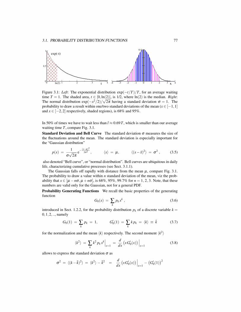
3.1. PROBABILITY DISTRIBUTION FUNCTIONS 77
0 1 2 3 4t0
0.5
1
exp(-t)
ln(2) -4 -3 -2 -1 0 1 2 3 4x
0.4
Figure 3.1: Left: The exponential distribution exp(−t/T )/T , for an average waitingtime T = 1. The shaded area, t ∈ [0, ln(2)], is 1/2, where ln(2) is the median. Right:The normal distribution exp(−x2/2)/
√2π having a standard deviation σ = 1. The
probability to draw a result within one/two standard deviations of the mean (x∈ [−1,1]and x ∈ [−2,2] respectively, shaded regions), is 68% and 95%.
In 50% of times we have to wait less than t ≈ 0.69T , which is smaller than our averagewaiting time T , compare Fig. 3.1.Standard Deviation and Bell Curve The standard deviation σ measures the size ofthe fluctuations around the mean. The standard deviation is especially important forthe “Gaussian distribution”
p(x) =1
σ√
2πe−
(x−µ)2
2σ2 , 〈x〉 = µ, 〈(x− x)2〉 = σ2 , (3.5)
also denoted “Bell curve”, or “normal distribution”. Bell curves are ubiquitous in dailylife, characterizing cumulative processes (see Sect. 3.1.1).
The Gaussian falls off rapidly with distance from the mean µ , compare Fig. 3.1.The probability to draw a value within n standard deviation of the mean, viz the prob-ability that x ∈ [µ−nσ ,µ +nσ ], is 68%, 95%, 99.7% for n = 1, 2, 3. Note, that thesenumbers are valid only for the Gaussian, not for a general PDF.Probability Generating Functions We recall the basic properties of the generatingfunction
G0(x) = ∑k
pk xk , (3.6)
introduced in Sect. 1.2.2, for the probability distribution pk of a discrete variable k =0,1,2, .., namely
G0(1) = ∑k
pk = 1, G′0(1) = ∑k
k pk = 〈k〉 ≡ k (3.7)
for the normalization and the mean 〈k〉 respectively. The second moment 〈k2〉
〈k2〉 = ∑k
k2 pk xk∣∣∣x=1
=ddx
(xG′0(x)
)∣∣∣x=1
(3.8)
allows to express the standard deviation σ as
σ2 = 〈(k− k)2〉 = 〈k2〉 − k2 =
ddx
(xG′0(x)
)∣∣∣x=1−(G′0(1)
)2

78 CHAPTER 3. COMPLEXITY AND INFORMATION THEORY
= G′′0(1) + G′0(1)−(G′0(1)
)2. (3.9)
The importance of probability generating functions lies in the fact that the distributionfor the sum k = ∑i ki of independent stochastic variables ki is generated by the productof the generating functions G(i)
0 (x) of the respective individual processes p(i)ki, viz
G0(x) = ∑k
pkxk = ∏i
G(i)0 (x), G(i)
0 (x) = ∑ki
p(i)kixki ,
see Sect. 1.2.2 for further details and examples.Bayesian Theorem Events and processes may have dependencies upon each other. Aphysician will typically have to know, to give an example, the probability that a patienthas a certain illness, given that the patient shows a specific symptom.
Conditional Probability. The probability that an event x occurs, giventhat an event y has happened, is denoted “conditional probability” p(x|y).
Throwing a dice twice, the probability that the first throw resulted in a 1, given that thetotal result was 4 = 1+3 = 2+2 = 3+1, is 1/3. Obviously,
p(x) =∫
p(x|y) p(y)dy (3.10)
holds. The probability distribution of throwing x in the first throw and y in the secondthrow is determined, on the other hand, by the joint distribution p(x,y).
Joint Probability Distribution. The probability of events x and y oc-curring is given by the “joint probability” p(x,y).
Note, that∫
p(x,y)dxdy = 1. The self-evident relation
p(x,y) = p(x|y) p(y) (3.11)
is denoted “Bayes’ theorem”. As a corollary of Eq. (3.11), p(y|x)p(x) = p(x|y)p(y)holds.
3.1.1 The Law of Large NumbersThrowing a dice many times and adding up the results obtained, the resulting averagewill be close to 3.5N, where N is the number of throws. This is the typical outcomefor cumulative stochastic processes5.
Law of Large Numbers. Repeating N times a stochastic process withmean x and standard deviation σ , the mean and the standard deviationof the cumulative result will approach xN and σ
√N respectively in the
thermodynamic limit N→ ∞.
5Please take note of the difference between a cumulative stochastic process, when adding the results ofindividual trials, and the “cumulative PDF” F(x) defined by F(x) =
∫ x−∞
p(x′)dx′.

3.1. PROBABILITY DISTRIBUTION FUNCTIONS 79
The law of large numbers implies, that one obtains x as an averaged result, with astandard deviation σ/
√N for the averaged process. One needs to square the number
of trials in order to improve accuracy by a factor of two.Proof For a proof of the law of large numbers we consider a discrete process pk de-scribed by the generating functional G0(x). This is not really a restriction, since PDFsof continuous variables can be discretized with arbitrary accuracy. The cumulativestochastic process is then characterized by a generating functional
GN0 (x), k(N) =
ddx
GN0 (x)
∣∣∣x=1
= N GN−10 (x)G′0(x)
∣∣∣x=1
= N k
and the mean k(N) = Nk respectively. For the standard deviation σ (N) of the cumulativeprocess we use Eq. (3.9),(
σ(N))2
=ddx
(x
ddx
GN0 (x)
)∣∣∣x=1−(Nk)2
=ddx
(xN GN−1
0 (x)G′0(x))∣∣∣
x=1− N2 (G′0(1))2
= NG′0(1) + N(N−1)(G′0(1)
)2+ NG′′0(1) − N2 (G′0(1))2
= N(
G′′0(1)+G′0(1)−(G′0(1)
)2)≡ N σ
2 , (3.12)
and obtain the law of large numbers.Central Limiting Theorem The law of large numbers tells us, that the variance σ2 isadditive for cumulative processes, not the standard deviation σ . The “central limitingtheorem” then tells us, that the limiting distribution function is a Gaussian.
Central Limiting Theorem. Given i = 1, . . . ,N independent randomvariables xi, distributed with mean µi and standard deviations σi. The cu-mulative distribution x = ∑i xi is then described, for N→∞, by a Gaussianwith mean µ = ∑i µi and variance σ2 = ∑i σ2
i .
In most cases one is not interested in the cumulative result, but in the averaged one,which is obtained by rescaling of variables
y = x/N, µ = µ/N, σ = σ/N, p(y) =1
σ√
2πe−
(y−µ)2
2σ2 .
The rescaled standard deviation scales with 1/√
N. To see this, just consider identicalprocesses with σi ≡ σ0,
σ =1N
√∑
iσ2
i =σ0√
N,
in accordance with the law of large numbers.Is Everything Boring Then? One might be tempted to draw the conclusion thatsystems containing a large number of variables are boring, since everything seems toaverage out. This is actually not the case, the law of large numbers holds only forstatistically independent processes. Subsystems of distributed complex systems arehowever dynamically dependent and these dynamical correlations may lead to highlynon-trivial properties in the thermodynamic limit.

80 CHAPTER 3. COMPLEXITY AND INFORMATION THEORY
0 0,2 0,4 0,6 0,8 1t0
2
4
6
xn+1
= rxn(1-x
n)
0
0,2
0,4
join
t p
rob
abil
itie
s
p++
p+-
p-+
p--
Figure 3.2: For the logistic map with r = 3.9 and x0 = 0.6, two statistical analysesof the time series xn, n = 0, . . . ,N, with N = 106. Left: The distribution p(x) of thexn. Plotted is Nbin p(x)/N, for Nbin = 10/100 bins (curve with square symbols andopen vertical bars respectively). The data is plotted at the midpoints of the respectivebins. Right: The joint probabilities p±±, as defined by Eq. (3.15), of consecutive in-creases/decreases of the xn. The probability p−− that the data decreases consecutivelytwice vanishes.
3.1.2 Time Series Characterization
In many cases one is interested in estimating the probability distribution functions fordata generated by some known or unknown process, like the temperature measurementsof a weather station. It is important, when doing so, to keep a few caveats in mind.
Binning of Variables Here we will be dealing mainly with the time series of datagenerated by dynamical systems. As an example we consider the logistic map, compareSect. 2.2,
xn+1 = f (xn) ≡ r xn (1− xn), xn ∈ [0,1], r ∈ [0,4] . (3.13)
The dynamical variable is continuous and in order to estimate the probability distribu-tion of the xn we need to bin the data. In Fig. 3.2 the statistics of a time series in thechaotic regime, for r = 3.9, is given.
One needs to select the number of bins Nbin and, in general, also the positions andthe widths of the bins. When the data is not uniformly distributed one may place morebins in the region of interest, generalizing the relation (3.1) through ∆x→ ∆xi, with the∆xi being the width of the individual bins.
For our illustrative example see Fig. 3.2, we have selected Nbin = 10/100 equidis-tant bins. The data is distributed over more bins, when Nbin increases. In order to makethe PDFs for different number of bins comparable one needs to rescale them with Nbin,as it has been done for the data shown in Fig. 3.2.
The selection of the binning procedure is in general a difficult choice. Fine structurewill be lost when Nbin is too low, but statistical noise will dominate for a too largenumber of bins.
Symbolization One denotes by “symbolization” the construction of a finite number of

3.1. PROBABILITY DISTRIBUTION FUNCTIONS 81
symbols suitable for the statistical characterization of a given time series6. The binningprocedure discussed above is a commonly used symbolization procedure.
For a further example of a symbolization procedure we denote with δt =±1,
δt = sign(xt − xt−1) =
1 xt > xt−1−1 xt < xt−1
(3.14)
the direction of the time development. The consecutive development of the δt may thenbe encoded in higher-level symbolic stochastic variables. E.g. one might be interestedin the joint probabilities
p++ = 〈p(δt = 1,δt−1 = 1)〉t p+− = 〈p(δt = 1,δt−1 =−1)〉tp−+ = 〈p(δt =−1,δt−1 = 1)〉t p−− = 〈p(δt =−1,δt−1 =−1)〉t
,
(3.15)where p++ gives the probability that the data increases at least twice consecutively, etc.,and where 〈. . .〉t denotes the time average. In Fig. 3.2 the values for the joint probabil-ities p±± are given for a selected time series of the logistic map in the chaotic regime.The data never decreases twice consecutively, p−− = 0, a somewhat unexpected result.
There are many possible symbolization procedures and the procedure used to an-alyze a given time series determines the kind of information one may hope to extract,as evident from the results illustrated in Fig. 3.2. The selection of the symbolizationprocedures needs to be given attention, and will be discussed further in Sect. 3.2.1.Self Averaging A time series produced by a dynamical system depends on the initialcondition and so will generally also the statistical properties of the time series. As anexample we consider the XOR series7
σt+1 = XOR(σt ,σt−1), σt = 0, 1 . (3.16)
The four initial conditions 00, 01, 10 and 11 give rise to the respective time series
. . .000000000 . . .101101101
. . .110110110 . . .011011011 (3.17)
where time runs from right to left and where we have underlined the initial condi-tion σ1 and σ0. The typical time series, occurring for 75% of the initial conditions,is ..011011011011.., with p(0) = 1/3 and p(1) = 2/3 for the probability to find a0/1. When averaging over all four initial conditions, we have on the other hand(2/3)(3/4) = 1/2 for the probability to find a 1. Then
p(1) =
2/3 typical1/2 average .
When observing a single time series we are likely to obtain the typical probability,analyzing many time series will result on the other hand in the average probability.
6For continuous-time data, as for an electrocardiogram, an additional symbolization step is necessary,the discretization of time. Here we consider however only discrete-time series.
7Remember, that XOR(0,0) = 0 = XOR(1,1) and XOR(0,1) = 1 = XOR(1,0).

82 CHAPTER 3. COMPLEXITY AND INFORMATION THEORY
Self Averaging. When the statistical properties of a time series gen-erated by a dynamical process are independent of the respective initialconditions, one says the time series is “self averaging”.
The XOR series is not self averaging and one can generally not assume self averagingto occur. An inconvenient situation whenever only a single time series is available, asit is the case for most historical data, e.g. of past climatic conditions.
XOR Series with Noise Most real-world processes involve a certain degree of noiseand one may be tempted to assume, that noise could effectively restart the dynam-ics, leading to an implicitly averaging over initial conditions. This assumption is notgenerally valid but works out for XOR process with noise,
σt+1 =
XOR(σt ,σt−1) probability 1−ξ
¬XOR(σt ,σt−1) probability ξ0≤ ξ 1 . (3.18)
For low level of noise, ξ → 0, the time series
. . .000000001101101101011011011011101101101100000000 . . .
has stretches of regular behavior interseeded by four types of noise induced dynamics(underlined, time running from right to left). Denoting with p000 and p011 the probabil-ity of finding regular dynamics of type ..000000000.. and ..011011011.. respectively,we find the master equation
p011 = ξ p000 − ξ p011/3 = −p000 (3.19)
for the noise-induced transition probabilities. In the stationary case p000 = p011/3 forthe XOR process with noise, the same ratio one would obtain for the deterministicXOR series averaged over the initial conditions.
The introduction of noise generally introduces a complex dynamics akin to themaster Eq. (3.19) and it is generally not to be expected that the time series becomessuch self-averaging. A simple counter example is the OR time series; we leave itsanalysis to the reader.
Time Series Analysis and Cognition Time series analysis is a tricky business when-ever the fundamentals of the generative process are unknown, e.g. whether noise is im-portant or not. This is however the setting in which cognitive systems, see Chap. 8, areoperative. Our sensory organs, eyes and ears, provide us with a continuous time seriesencoding environmental information. Performing an informative time series analysisis paramount for surviving.
3.2 Entropy and InformationEntropy is a venerable concept from physics encoding the amount of disorder presentin a thermodynamic system at a given temperature. The “Second Law of Thermo-dynamics” states, that entropy can only increase in an isolated (closed) system. Thesecond law has far reaching consequences, e.g. determining the maximal efficiency of

3.2. ENTROPY AND INFORMATION 83
engines and power plants, and philosophical implications for our understanding of thefundamentals underpinning the nature of life as such.Entropy and Life Living organisms have a body and such create ordered structuresfrom basic chemical constituents. Living beings therefore decrease entropy locally, intheir bodies, seemingly in violation of the second law. In reality, the local entropydepressions are created on the expense of corresponding entropy increases in the envi-ronment, in agreement with the second law of thermodynamics. All living beings needto be capable of manipulating entropy.Information Entropy and Predictability Entropy is also a central concept in in-formation theory, where it is commonly denoted “Shannon entropy” or “informationentropy”. In this context one is interested in the amount of information encoded by asequence of symbols
. . .σt+2, σt+1, σt , σt−1, σt−2, . . . ,
e.g. when transmitting a message. Typically, in everyday computers, the σt are wordsof bits. Let us consider two time series of bits, e.g.
. . .101010101010 . . . , . . .1100010101100 . . . . (3.20)
The first example is predictable, from the perspective of a time-series, and ordered,from the perspective of an one-dimensional alignment of bits. The second example isunpredictable and disordered respectively.
Information can be transmitted through a time series of symbols only when thistime series is not predictable. Talking to a friend, to illustrate this statement, we willnot learn anything new when capable of predicting his next joke. We have thereforethe following two perspectives,
high entropy =
large disorder physics
high information content information theory ,
and vice versa. Only seemingly disordered sequences of symbols are unpredictableand thus potential carriers of information. Note, that the predictability of a given timeseries, or its degree of disorder, may not necessarily be as self evident as in above ex-ample, Eq. (3.20), depending generally on the analysis procedure used, see Sect. 3.2.1.Extensive Information In complex system theory, as well as in physics, we are ofteninterested in properties of systems composed of many subsystems.
Extensive and Intensive Properties. For systems composed of N sub-systems a property is denoted “extensive” if it scales as O(N1) and “inten-sive” when it scales with O(N0).
A typical extensive property is the mass, a typical intensive property the density. Whenlumping together two chunks of clay, their mass adds, but the density does not change.
One demands, both in physics and in information theory, that the entropy should bean extensive quantity. The information content of two independent transmission chan-nels should be just the sum of the information carried by the two individual channels.
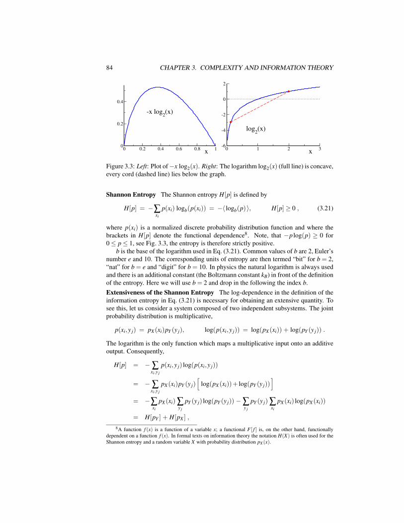
84 CHAPTER 3. COMPLEXITY AND INFORMATION THEORY
0 0.2 0.4 0.6 0.8 1x0
0.2
0.4
-x log2(x)
0 1 2 3x
-6
-4
-2
0
2
log2(x)
Figure 3.3: Left: Plot of−x log2(x). Right: The logarithm log2(x) (full line) is concave,every cord (dashed line) lies below the graph.
Shannon Entropy The Shannon entropy H[p] is defined by
H[p] = −∑xi
p(xi) logb(p(xi)) = −〈 logb(p)〉, H[p]≥ 0 , (3.21)
where p(xi) is a normalized discrete probability distribution function and where thebrackets in H[p] denote the functional dependence8. Note, that −p log(p) ≥ 0 for0≤ p≤ 1, see Fig. 3.3, the entropy is therefore strictly positive.
b is the base of the logarithm used in Eq. (3.21). Common values of b are 2, Euler’snumber e and 10. The corresponding units of entropy are then termed “bit” for b = 2,“nat” for b = e and “digit” for b = 10. In physics the natural logarithm is always usedand there is an additional constant (the Boltzmann constant kB) in front of the definitionof the entropy. Here we will use b = 2 and drop in the following the index b.Extensiveness of the Shannon Entropy The log-dependence in the definition of theinformation entropy in Eq. (3.21) is necessary for obtaining an extensive quantity. Tosee this, let us consider a system composed of two independent subsystems. The jointprobability distribution is multiplicative,
p(xi,y j) = pX (xi)pY (y j), log(p(xi,y j)) = log(pX (xi)) + log(pY (y j)) .
The logarithm is the only function which maps a multiplicative input onto an additiveoutput. Consequently,
H[p] = −∑xi,y j
p(xi,y j) log(p(xi,y j))
= −∑xi,y j
pX (xi)pY (y j)[
log(pX (xi))+ log(pY (y j))]
= −∑xi
pX (xi) ∑y j
pY (y j) log(pY (y j)) −∑y j
pY (y j) ∑xi
pX (xi) log(pX (xi))
= H[pY ] + H[pX ] ,
8A function f (x) is a function of a variable x; a functional F [ f ] is, on the other hand, functionallydependent on a function f (x). In formal texts on information theory the notation H(X) is often used for theShannon entropy and a random variable X with probability distribution pX (x).

3.2. ENTROPY AND INFORMATION 85
as necessary for the extensiveness of H[p]. Hence the log-dependence in Eq. (3.21).
Degrees of Freedom We consider a discrete system with xi ∈ [1, . . . ,n], having n“degrees of freedom” in physics’ slang. If the probability of finding any value is equallylikely, as it is the case for a thermodynamic system at infinite temperatures, the entropyis
H = −∑xi
p(xi) log(p(xi)) = −n1n
log(1/n) = log(n) , (3.22)
a celebrated result. The entropy grows logarithmically with the number of degrees offreedom.
Shannon’s Source Coding Theorem So far we have shown, that Eq. (3.21) is the onlypossible definition, modulo renormalizing factors, for an extensive quantity dependingexclusively on the probability distribution. The operative significance of the entropyH[p] in terms of informational content is given by Shannon’s theorem.
Source Coding Theorem. Given a random variable x with a PDF p(x)and entropy H[p]. The cumulative entropy NH[p] is then, for N → ∞, alower bound for the number of bits necessary when trying to compress Nindependent processes drawn from p(x).
If we compress more, we will lose information, the entropy H[p] is therefore a measureof information content.
Entropy and Compression Let’s make an example. Consider we have words madeout of the four letter alphabet A, B, C and D. Suppose, that these four letters would notoccur with the same probability, the relative frequencies being
p(A) =12, p(B) =
14, p(C) =
18= p(D) .
When transmitting a long series of words using this alphabet we will have the entropy
H[p] =−12
log(1/2) − 14
log(1/4) − 18
log(1/8) − 18
log(1/8)
=12+
24+
38+
38
= 1.75 , (3.23)
since we are using the logarithm with base b = 2. The most naive bit encoding,
A→ 00, B→ 01, C→ 10, D→ 11 ,
would use exactly two bit, which is larger than the Shannon entropy. An optimal en-coding would be, on the other hand,
A→ 1, B→ 01, C→ 001, D→ 000 , (3.24)
leading to an average length of words transmitted of
p(A) + 2p(B) + 3p(C) + 3p(D) =12+
24+
38+
38
= 1.75 , (3.25)

86 CHAPTER 3. COMPLEXITY AND INFORMATION THEORY
which is the same as the information entropy H[p]. The encoding given in Eq. (3.24)is actually “prefix-free”. When we read the words from left to right, we know where anew word starts and stops,
110000010101 ←→ AADCBB ,
without ambiguity. Fast algorithms for optimal, or close to optimal encoding are clearlyof importance in the computer sciences and for the compression of audio and videodata.
Discrete vs. Continuous Variables When defining the entropy we have consideredhitherto discrete variables. The information entropy can also be defined for continousvariables. We should be careful though, being aware that the transition from continuousto discrete stochastic variables, and vice versa, is slightly non-trivial, compare Eq.(3.1):
H[p]∣∣∣con
= −∫
p(x) log(p(x))dx ≈ ∑i
p(xi) log(p(xi)))∆x
= −∑i
pi log(pi/∆x) = −∑i
pi log(pi) + ∑i
pi log(∆x)
= H[p]∣∣∣dis
+ log(∆x) , (3.26)
where pi = p(xi)∆x is here the properly normalized discretized PDF, compare Eq. (3.1).The difference log(∆x) between the continuous-variable entropy H[p]
∣∣con and the dis-
cretized version H[p]∣∣dis diverges for ∆x→ 0, the transition is discontinuous.
Entropy of a Continuous PDF From Eq. (3.26) it follows, that the Shannon en-tropy H[p]
∣∣con can be negative for a continous probability distribution function. As an
example consider the flat distribution
p(x) =
1/ε for x ∈ [0, ε]
0 otherwise ,∫ ε
0p(x)dx = 1
in the small interval [0, ε], with the entropy
H[p]∣∣∣con
= −∫ ε
0
1ε
log(1/ε)dx = log(ε) < 0, for ε < 1 .
The absolute value of the entropy is hence not meaningful for continous PDFs, onlyentropy differences. H[p]
∣∣con is therefore also referred-to as “differential entropy”.
Maximal Entropy Distributions Which kind of distributions maximize entropy, vizinformation content? Remembering that
limp→0,1
p log(p) = 0, log(1) = 0 ,
see Fig. 3.3, it is intuitive that a flat distribution might be optimal. This is indeed correctin the absence of any further constraints. We consider three cases.
3.2. ENTROPY AND INFORMATION 87
– No constraint: we need to maximize
H[p] =∫
f (p(x))dx, f (p) = −p log(p) , (3.27)
where the notation used will turn out useful later on. Maximizing a functionallike H[p] is a typical task of variational calculus. One considers with
p(x) = popt(x) + δ p(x), δ p(x) arbitrary
a general variation of δ p(x) around the optimal function popt(x). At optimality,the dependence of H[p] on the variation δ p should be stationary,
0 ≡ δH[p] =∫
f ′(p)δ pdx, 0 = f ′(p) , (3.28)
where f ′(p) = 0 follows from the fact that δ p is an arbitrary function. Forf (p) =−p log(p) we find then with
f ′(p) = − log(p)−1 = 0, p(x) = const. (3.29)
the expected flat distribution.
– Fixed mean: next we consider the entropy maximization under the constraint offixed average µ ,
µ =∫
x p(x)dx . (3.30)
This condition can be enforced by a Lagrange parameter λ via
f (p) = −p log(p) − λxp .
The stationary condition f ′(p) = 0 then leads to
f ′(p) = − log(p)−1−λx = 0, p(x) ∝ 2−λx ∼ e−x/µ (3.31)
the exponential distribution, see Eq. (3.4), with mean µ . The Lagrange parameterλ needs to be determined such that the condition of fixed mean, Eq. (3.30), issatisfied. For a support x ∈ [0,∞], as assumed above, we have λ loge(2) = 1/µ .
– Fixed mean and variance: Lastly we consider the entropy maximization underthe constraint of fixed average µ and variance σ2,
µ =∫
x p(x)dx, σ2 =
∫(x−µ)2 p(x)dx . (3.32)
We leave it to the reader to show that the entropy is the maximal for a Gaussian.

88 CHAPTER 3. COMPLEXITY AND INFORMATION THEORY
3.2.1 Information Content of a Real-World Time SeriesThe Shannon entropy is a very powerful concept in information theory. The encodingrules are typically known in information theory, there is no ambiguity regarding thesymbolization procedure (see Sect. 3.1.2) to employ when receiving a message viasome technical communication channel. This is however not any more the case, whenwe are interested in determining the information content of real-world processes, e.g.the time series of certain financial data or the data stream produced by our sensoryorgans.
Symbolization and Information Content The result obtained for the informationcontent of a real-world time series σt depends in general on the symbolization pro-cedure used. Let us consider, as an example, the first time series of Eq. (3.20),
. . .101010101010 . . . . (3.33)
When using a one-bit symbolization procedure, we have
p(0) =12= p(1), H[p] = −2
12
log(1/2) = 1 ,
as expected. If, on the other hand, we use a two-bit symbolization, we find
p(00) = p(11) = p(01) = 0, p(10) = 1, H[p] = − log(1) = 0 .
When two-bit encoding is presumed, the time series is predictable and carries no infor-mation. This seems intuitively the correct result and the question is: Can we formulatea general guiding principle which tells us which symbolization procedure would yieldthe more accurate result for the information content of a given time series?
The Minimal Entropy Principle The Shannon entropy constitutes a lower boundfor the number of bits, per symbol, necessary when compressing the data without lossof information. Trying various symbolization procedures, the symbolization procedureyielding the lowest information entropy then allows us to represent, without loss ofinformation, a given time series with the least number of bits.
Minimal Entropy Principle. The information content of a time serieswith unknown encoding is given by the minimum (actually the infimum)of the Shannon entropy over all possible symbolization procedures.
The minimal entropy principle then gives us a definite answer with respect to the in-formation content of the time series given in Eq. (3.33). We have seen that at least onesymbolization procedure yields a vanishing entropy and one cannot get a lower value,since H[p]≥ 0. This is the expected result, since ..01010101.. is predictable.
Information Content of a Predictable Time Series Note, that a vanishing informa-tion content H[p] = 0 only implies that the time series is strictly predictable, not that itis constant. One therefore needs only a finite amount of information to encode the fulltime series, viz for arbitrary lengths N → ∞. When the time series is predictable, theinformation necessary to encode the series is intensive and not extensive.

3.2. ENTROPY AND INFORMATION 89
Symbolization and Time Horizons The minimal entropy principle is rather abstract.In practice one may not be able than to try out more than a handful of different symbol-ization procedures. It is therefore important to gain an understanding of the time seriesat hand.
An important aspect of many time series is the intrinsic time horizon τ . Mostdynamical processes have certain characteristic time scales and memories of past statesare effectively lost for times exceeding these intrinsic time scales. The symbolizationprocedure used should therefore match the time horizon τ
This is what happened when analyzing the time series given in Eq. (3.33), for whichτ = 2. A one-bit symbolization procedure implicitly presumes that σt and σt+1 arestatistically independent and such missed the intrinsic time scale τ = 2, in contrast tothe two-bit symbolization procedure.
3.2.2 Mutual InformationWe have been considering so far the statistical properties of individual stochastic pro-cesses as well as the properties of cumulative processes generated by the sum of stochas-tically independent random variables. In order to understand complex systems we needto develop tools for the description of a large number of interdependent processes. As afirst step towards this direction we consider in the following the case of two stochasticprocesses, which may now be statistically correlated.Two Channels - Markov Process We start by considering an illustrative example oftwo correlated channels σt and τt , with
σt+1 = XOR(σt ,τt), τt+1 =
XOR(σt ,τt) probability 1−ξ
¬XOR(σt ,τt) probability ξ.
(3.34)This dynamics has the “Markov property”, the value for the state σt+1,τt+1 dependsonly on the state at the previous time step, viz on σt ,τt.
Markov Process. A discrete-time memory-less dynamical process isdenoted a “Markov process”. The likelihood of future states depends onlyon the present state, and not on any past states.
When the state space is finite, as in our example, the term “Markov chain” is also used.We will not adhere here to the distinction which is sometimes made between discreteand continuous time, with Markov processes being formulated for discrete time and“master equations” describing stochastic processes for continuous time.Joint Probabilities A typical time series of the Markov chain specified in Eq. (3.34)looks like
. . .σt+1σt . . . : 00010000001010 . . .. . .τt+1τt . . . : 00011000001111 . . . ,
where we have underlined instances of noise-induced transitions. For ξ = 0 the station-ary state is σt ,τt= 0,0 and therefore fully correlated. We now calculate the jointprobabilities p(σ ,τ) for general values of noise ξ , using the transition probabilities
pt+1(0,0) = (1−ξ ) [pt(1,1)+ pt(0,0)]pt+1(1,1) = (1−ξ ) [pt(1,0)+ pt(0,1)]
,pt+1(1,0) = ξ [pt(0,1)+ pt(1,0)]pt+1(0,1) = ξ [pt(0,0)+ pt(1,1)]
,

90 CHAPTER 3. COMPLEXITY AND INFORMATION THEORY
0 0.1 0.2 0.3 0.4 0.5 ξ0
0.5
1
1.5
2
entr
opy [
bit
]
H[pσ]
H[pτ]
H[pσ] + H[p
τ] H[p]
Figure 3.4: For the two-channel XOR-Markov chain σt ,τt with noise ξ , see Eq.(3.34), the entropy H[p] of the combined process (full line, Eq. (3.38)), of the indi-vidual channels (dashed lines, Eq. (3.37)), H[pσ ] and H[pτ ], and of the sum of thejoint entropies (dot-dashed line). Note the positiveness of the mutual information,I(σ ,τ) = H[pσ ]+H[pτ ]−H[p]> 0.
for the ensemble averaged joint probability distributions pt(σ ,τ)= 〈p(σt ,τt)〉ens, wherethe average 〈..〉ens denotes the average over an ensemble of time series. For the solutionin the stationary case pt+1(σ ,τ) = pt(σ ,τ)≡ p(σ ,τ) we use the normalization
p(1,1) + p(0,0) + p(1,0) + p(0,1) = 1 .
We findp(1,1) + p(0,0) = 1−ξ , p(1,0) + p(0,1) = ξ ,
by adding the terms ∝ (1−ξ ) and ∝ ξ respectively. It then follows immediately
p(0,0) = (1−ξ )2
p(1,1) = (1−ξ )ξ,
p(1,0) = ξ 2
p(0,1) = ξ (1−ξ ). (3.35)
For ξ = 1/2 the two channels become 100% uncorrelated, as the τ-channel is then fullyrandom. The dynamics of the Markov process given in Eq. (3.34) is self averaging andit is illustrative to verify the result for the joint PDF, Eq. (3.35), by a straightforwardnumerical simulation.Entropies Using the notation
pσ (σ′) = ∑
τ ′p(σ ′,τ ′), pτ(τ
′) = ∑σ ′
p(σ ′,τ ′)
for the “marginal PDFs” pσ and pτ , we find from Eq. (3.35)
pσ (0) = 1−ξ
pσ (1) = ξ,
pτ(0) = 1−2ξ (1−ξ )pτ(1) = 2ξ (1−ξ )
(3.36)
for the PDFs of the two individual channels. We may now evaluate both the entropiesof the individual channels, H[pσ ] and H[pτ ], the “marginal entropies”, viz
H[pσ ] = −〈log(pσ )〉, H[pτ ] = −〈log(pτ)〉 , (3.37)

3.2. ENTROPY AND INFORMATION 91
as well as the entropy of the combined process, termed “joint entropy”,
H[p] = − ∑σ ′,τ ′
p(σ ′,τ ′) log(p(σ ′,τ ′)) . (3.38)
In Fig. 3.4 the respective entropies are plotted as a function of noise strength ξ . Someobservations:
• In the absence of noise, ξ = 0, both the individual channels as well as the com-bined process are predictable and all three entropies, H[p], H[pσ ] and H[pτ ],vanish consequently.
• For maximal noise ξ = 0.5, the information content of both individual chains isone bit and of the combined process two bits, implying statistical independence.
• For general noise strengths 0< ξ < 0.5, the two channels are statistically corre-lated. The information content of the combined process H[p] is consequentlysmaller than the sum of the information contents of the individual channels,H[pσ ]+H[pτ ].
Mutual Information The degree of statistical dependency of two channels can bemeasured by comparing the joint entropy with the respective marginal entropies.
Mutual Information. For two stochastic processes σt and τt thedifference
I(σ ,τ) = H[pσ ]+H[pτ ]−H[p] (3.39)
between the sum of the marginal entropies H[pσ ] +H[pτ ] and the jointentropy H[p] is denoted “mutual information” I(σ ,τ).
When two dynamical processes become correlated, information is lost and this infor-mation loss is given by the mutual information. Note, that I(σ ,τ) = I[p] is a functionalof the joint probability distribution p only, the marginal PDFs pσ and pτ being them-selves functionals of p.Positiveness We will now discuss some properties of the mutual information, consid-ering the general case of two stochastic processes described by the joint PDF p(x,y)and the respective marginal PDFs pX (x) =
∫p(x,y)dy, pY (y) =
∫p(x,y)dx.
The mutual information
I(X ,Y ) = 〈log(p)〉 − 〈log(pX )〉 − 〈log(pY )〉 I(X ,Y ) ≥ 0 , (3.40)
is strictly positive. Rewriting the mutual information as
I(X ,Y ) =∫
p(x,y)[
log(p(x,y))− log(pX (x))− log(pY (y))]dxdy (3.41)
=∫
p(x,y) log(
p(x,y)pX (x)pY (y)
)dxdy = −
∫p log
(pX pY
p
)dxdy ,
we can easily show that I(X ,Y ) ≥ 0 follows from the concaveness of the logarithm,see Fig. 3.3,
log(p1x1 + p2x2) ≥ p1 log(x1)+ p2 log(x2), ∀x1,x2 ∈ [0,∞] , (3.42)

92 CHAPTER 3. COMPLEXITY AND INFORMATION THEORY
and p1, p2 ∈ [0,1], with p1 + p2 = 1; any cord of a concave function lies below thegraph. We can regard p1 and p2 as the coefficients of a distribution function and gen-eralize,
p1δ (x− x1)+ p2δ (x− x2) −→ p(x) ,
where p(x) is now a generic, properly normalized PDF. The concaveness condition,Eq. (3.42), then reads
log(∫
p(x)xdx))≥∫
p(x) log(x)dx , ϕ (〈x〉) ≥ 〈ϕ(x)〉 , (3.43)
the “Jensen inequality”, which holds for any concave function ϕ(x). This inequalityremains valid when substituting x→ pX pY/p for the argument of the logarithm9. Wethen obtain for the mutual information, Eq. (3.41),
I(X ,Y ) = −∫
p log(
pX pY
p
)dxdy ≥ − log
(∫ppX pY/pdxdy
)= − log
(∫pX (x)dx
∫pY (y)dy
)= − log(1) = 0 ,
viz I(X ,Y ) is non-negative. Information can only be loost when correlating two previ-ously independent processes.Conditional Entropy There are various ways to rewrite the mutual information, usingBayes theorem p(x,y) = p|(x|y)pY (y) between the joint PDF p(x,y), the conditionalPDF p|(x|y) and the marginal PDF pY (y), e.g.
I(X ,Y ) =
⟨log(
ppX pY
)⟩=∫
p(x,y) log(
p(x|y)pX (x)
)dxdy
≡ H[pX ] − H[p|] ,
where we have defined the “conditional entropy”
H[p|] = −〈 log(p|)〉 = −∫
p(x,y) log(p|(x|y))dxdy . (3.44)
The conditional entropy is positive for discrete processes, since
−p(xi,y j) log(p|(xi|y j)) = −p|(xi|y j)pY (y j) log(p|(xi|y j))
is positive, as−p| log(p|)≥ 0 in the interval p| ∈ [0,1], compare Fig. 3.3 and Eq. (3.26)for the change-over from continous to discrete variables. Several variants of the condi-tional entropy may be used to extend the statistical complexity measures discussed inSect. 3.3.1.Kullback-Leibler Divergence The mutual information, Eq. (3.41), is a special caseof the “Kullback-Leibler Divergence”
9For a proof consider the generic substitution x→ q(x) and a transformation of variables x→ q viadx = dq/q′, with q′ = dq(x)/dx, for the integration in Eq. (3.43).

3.3. COMPLEXITY MEASURES 93
Kullback-Leibler Divergence. Given two probability distribution func-tions p(x) and q(x) the functional
K[p;q] =∫
p(x) log(
p(x)q(x)
)dx ≥ 0 (3.45)
is a non-symmetric measure of the difference between p(x) and q(x).
The Kullback-Leibler divergence K[p;q] is also denoted “relative entropy” and theproof for K[p;q] ≥ 0 is analogous to the one for the mutual information given above.The Kullback-Leibler divergence vanishes for p(x)≡ q(x).Example As a simple example we consider two distributions, p(σ) and q(σ), for abinary variable σ = 0,1,
p(0) = 1/2 = p(1), q(0) = α, q(1) = 1−α , (3.46)
with p(σ) being flat and α ∈ [0,1]. The Kullback-Leibler divergence,
K[p;q] = ∑σ=0,1
p(σ) log(
p(σq(σ)
)=−12
log(2α) − 12
log(2(1−α))
= − log(4(1−α)α)/2 ≥ 0 ,
is unbounded, since limα→0,1 K[p;q]→ ∞. Interchanging p↔ q we find
K[q; p] = α log(2α) + (1−α) log(2(1−α))
= log(2) + α log(α) + (1−α) log(1−α) ≥ 0 ,
which is now finite in the limit limα→0,1. The Kullback-Leibler divergence is highlyasymmetric, compare Fig. 3.5.
3.3 Complexity MeasuresCan we provide a single measure, or a small number of measures, suitable for char-acterizing the “degree of complexity” of any dynamical system at hand? This ratherphilosophical question has fascinated researchers for decades and no definitive answeris known.
The quest of complexity measures touches many interesting topics in dynamicalsystem theory and has led to a number of powerful tools suitable for studying dynam-ical systems, the original goal of developing a one-size-fit-all measure for complexityseems however not anymore a scientifically valid target. Complex dynamical systemscan show a huge variety of qualitatively different behaviors, one of the reasons whycomplex system theory is so fascinating, and it is not appropriate to shove all complexsystems into a single basket for the purpose of measuring their degree of complexitywith a single yardstick.Intuitive Complexity The task of developing a mathematically well defined measurefor complexity is handicapped by the lack of a precisely defined goal. In the following

94 CHAPTER 3. COMPLEXITY AND INFORMATION THEORY
0 0,5 1 α
1
2
3
K[p;q]
K[q;p]
complexity
order disorder
Figure 3.5: Left: For the two PDFs p and q parametrized by α , see Eq. (3.46), therespective Kullback-Leibler divergences K[p;q] (dashed line) and K[q; p] (full line).Note the maximal asymmetry for α → 0,1, where limα→0,1 K[p;q] = ∞. Right: Thedegree of complexity (full line) should be minimal both in the fully ordered and thefully disordered regime. For some applications it may however be meaningful to con-sider complexity measures maximal for random states (dashed line).
we will discuss some selected prerequisites and constraints one may postulate for avalid complexity measure. In the end it is, however, up to our intuition for decidingwhether these requirements are appropriate or not.
An example of a process one may intuitively attribute a high degree of complexityare the intricate spatio-temporal patterns generated by the forest fire model discussedin Sect. 5.3, and illustrated in Fig. 5.6, with perpetually changing fronts of fires burningthrough a continuously regrowing forest.
Complexity vs. Randomness A popular proposal for a complexity measure is theinformation entropy H[p], see Eq. (3.21). It vanishes when the system is regular, whichagrees with our intuitive presumption that complexity is low when nothing happens.The entropy is however maximal for random dynamics, as shown in Fig. 3.4.
It is a question of viewpoints to which extend one should consider random systemsas complex, compare Fig. 3.5. For some considerations, e.g. when dealing with “algo-rithmic complexity” (see Sect. 3.3.2) it makes sense to attribute maximal complexitydegrees to completely random sets of objects. In general, however, complexity mea-sures should be concave and minimal for regular behavior as well as for purely randomsequences.
Complexity of Multi-Component Systems Complexity should be a positive quantity,like entropy. Should it be, however, extensive or intensive? This is a difficult and highlynon-trivial question to ponder.
Intuitively one may demand complexity to be intensive, as one would not expect togain complexity when considering the behavior of a set of N independent and identicaldynamical systems. On the other side we cannot rule out that N strongly interactingdynamical systems could show more and more complex behavior with an increasingnumber of subsystems, e.g. we consider intuitively the global brain dynamics to beorders of magnitude more complex than the firing patterns of the individual neurons.
There is no simple way out of this quandary when searching for a single one-size-

3.3. COMPLEXITY MEASURES 95
fits-all complexity measure. Both intensive and extensive complexity measures havetheir areas of validity.Complexity and Behavior The search for complexity measures is not just an abstractacademic quest. As an example consider how bored we are when our environment isrepetitive, having low complexity, and how stressed when the complexity of our sen-sory inputs is too large. There are indeed indications that a valid behavioral strategy forhighly developed cognitive systems may consist in optimizing the degree of complex-ity. Well defined complexity measures are necessary in order to quantify this intuitivestatement mathematically.
3.3.1 Complexity and PredictabilityInteresting complexity measures can be constructed using statistical tools, generalizingconcepts like information entropy and mutual information. We will consider here timeseries generated from a finite set of symbols. One may, however, interchange the timelabel with a space label in the following, whenever one is concerned with studying thecomplexity of spatial structures.Stationary Dynamical Processes As a prerequisite we need stationary dynamicalprocesses, viz dynamical processes which do not change their behavior and their sta-tistical properties qualitatively over time. In practice this implies that the time seriesconsidered, as generated by some dynamical system, has a finite time horizon τ . Thesystem might have several time scales τi ≤ τ , but for large times t τ all correla-tion functions need to fall off exponentially, like the autocorrelation function definedin Sect. 5.2. Note, that this assumption may break down for critical dynamical sys-tems, which are characterized, as discussed in Chap. 5, by dynamical and statisticalcorrelations decaying only slowly, with an inverse power of time.Measuring Joint Probabilities For times t0, t1, .., a set of symbols X , and a timeseries containing n elements,
xn, xn−1, . . . , x2, x1, xi = x(ti), xi ∈ X (3.47)
we may define the joint probability distribution
pn : p(xn, . . . ,x1) . (3.48)
The joint probability p(xn, . . . ,x1) is not given a priori. It needs to be measured froman ensemble of time series. This is a very demanding task as p(xn, . . . ,x1) has (Ns)
n
components, with Ns being the number of symbols in X .It clearly makes no sense to consider joint probabilities pn for time differences
tn τ , the evaluation of joint probabilities exceeding the intrinsic time horizon τ is awaste of effort. In practice finite values of n are considered, taking subsets of length nof a complete time series containing normally a vastly larger number of elements. Thisis an admissible procedure for stationary dynamical processes.Entropy Density We recall the definition of the Shannon entropy
H[pn] = − ∑xn,..,x1∈X
p(xn, . . . ,x1) log(p(xn, . . . ,x1)) ≡ −〈 log(pn)〉pn , (3.49)

96 CHAPTER 3. COMPLEXITY AND INFORMATION THEORY
n
E
H[pn]
Figure 3.6: The entropy (full line) H[pn] of a time series of length n increases mono-tonically, with the limiting slope (dashed line) h∞. For large n → ∞ the entropyH[pn] ≈ E +h∞n, with the excess entropy E given by the intercept of asymptote withthe y-axis.
which needs to be measured for an ensemble of time series of length n or greater. Ofinterest is the entropy density in the limit of large times,
h∞ = limn→∞
1n
H[pn] , (3.50)
which exists for stationary dynamical processes with finite time horizons. The entropydensity is the mean number of bits per time step needed for encoding the time seriesstatistically.
Excess Entropy We define the “excess entropy” E as
E = limn→∞
(H[pn] − nh∞
)≥ 0 . (3.51)
The excess entropy is just the non-extensive part of the entropy, it is the coefficient ofthe term ∝ n0 when expanding the entropy in powers of 1/n,
H[pn] = nh∞ + E + O(1/n), n → ∞ , (3.52)
compare Fig. 3.6. The excess entropy E is positive as long as H[pn] is concave asa function of n (we leave the proof of this statement as an exercise to the reader),which is the case for stationary dynamical processes. For practical purposes one mayapproximate the excess entropy via
h∞ = limn→∞
hn, hn = H[pn+1] − H[pn] , (3.53)
since h∞ corresponds to the asymptotic slope of H[pn], compare Fig. 3.6.
• One may also use Eqs. (3.53) and (3.44) for rewriting the entropy density hn interms of an appropriately generalized conditional entropy.

3.3. COMPLEXITY MEASURES 97
• Using Eq. (3.52) we may rewrite the excess entropy as
∑n
[H[pn]
n−h∞
].
In this form the excess entropy is known as the “effective measure complexity”(EMC) or “Grassberger entropy”.
Excess Entropy and Predictability The excess entropy vanishes both for a randomand for an ordered system. For a random system
H[pn] = nH[pX ] ≡ nh∞ ,
where pX is the marginal probability. The excess entropy, Eq. (3.51) vanishes conse-quently. For an example of a system with ordered states we consider the dynamics
. . .000000000000000 . . . , . . .111111111111111 . . . ,
for a binary variable, occurring with probabilities α and 1−α respectively. This kindof dynamics is the natural output of logical AND or OR rules. The joint PDFs thenhave only two non-zero components,
p(0, . . . ,0) = α, p(1, . . . ,1) = 1−α, ∀n ,
all other p(xn, ..,x1) vanish and
H[pn] ≡ −α log(α) − (1−α) log(1−α), ∀n .
The entropy density h∞ vanishes and the excess entropy E becomes H[pn]; it vanishesfor α → 0,1, viz in the deterministic limit.
The excess entropy therefore fulfills the concaveness criteria illustrated in Fig. 3.5,vanishing both in the absence of predictability (random states) and for the case of strongpredictability (i.e. for deterministic systems). The excess entropy does however notvanish in above example for 0< α < 1, when two predictable states are superimposedstatistically in an ensemble of time series. Whether this behavior is compatible withour intuitive notion of complexity is, to a certain extent, a matter of taste.Discussion The excess entropy is a nice tool for time series analysis, satisfying severalbasic criteria for complexity measures, and there is a plethora of routes for furtherdevelopments, e.g. for systems showing structured dynamical activity both in the timeas well as in the spatial domain. The excess entropy is however exceedingly difficultto evaluate numerically and its scope of applications therefore limited to theoreticalstudies.
3.3.2 Algorithmic and Generative ComplexityWe have discussed so far descriptive approaches using statistical methods for the con-struction of complexity measures. One may, on the other hand, be interested in mod-elling the generative process. The question is then: which is the simplest model able toexplain the observed data?
98 CHAPTER 3. COMPLEXITY AND INFORMATION THEORY
Individual Objects For the statistical analysis of a time series we have been con-cerned with ensembles of time series, as generated by the identical underlying dynam-ical system, as well as with the limit of infinitely long times. In this section we will bedealing with individual objects composed of a finite number of n symbols, like
0000000000000000000000, 0010000011101001011001 .
The question is then: which dynamical model can generate the given string of symbols?One is interested, in particular, in strings of bits and in computer codes capable ofreproducing them.Turing Machine The reference computer codes in theoretical informatics is the setof instructions needed for a “Turing machine” to carry out a given computation. Theexact definition for a Turing machine is not of relevance here, it is essentially a finite-state machine working on a set of instructions called code. The Turing machine playsa central role in the theory of computability, e.g. when one is interested in examininghow hard it is to find the solution to a given set of problems.Algorithmic Complexity The notion of algorithmic complexity tries to find an an-swer to the question of how hard it is to reproduce a given time series in the absence ofprior knowledge.
Algorithmic Complexity. The “algorithmic complexity” of a string ofbits is the length of the shortest program that prints the given string of bitsand then halts.
The algorithmic complexity is also called “Kolmogorov complexity”. Note, that theinvolved computer or Turing machine is supposed to start with a blank memory, vizwith no prior knowledge.Algorithmic Complexity and Randomness Algorithmic complexity is a very pow-erful concept for theoretical considerations in the context of optimal computability. Ithas, however, two drawbacks, being not computable and attributing maximal complex-ity to random sequences.
A random number generator can only be approximated by any finite state machinelike the Turing machine and would need an infinite code length to be perfect. Thatis the reason why real-world codes for random number generators are producing only“pseudo random numbers”, with the degree of randomness to be tested by variousstatistical measures. Algorithmic complexity therefore conflicts with the common pos-tulate for complexity measures to vanish for random state, compare Fig. 3.5.Deterministic Complexity There is a vast line of research trying to understand thegenerative mechanism of complex behavior not algorithmically but from the perspec-tive of dynamical system theory, in particular for deterministic systems. The questionis then: in the absence of noise, which are the features needed to produce interestingand complex trajectories?
Of interest are in this context the sensitivity to initial condition for systems havinga transition between chaotic and regular states in phase space, see Chap. 4, the effectof bifurcations and non-trivial attractors like strange attractors, see Chap. 2, and theconsequences of feedback and tendencies toward synchronization, see Chap. 7. This

Exercises 99
line of research is embedded in the general quest of understanding the properties andthe generative causes of complex and adaptive dynamical systems.
Complexity and Emergence Intuitively, we attribute a high degree of complexityto ever changing structure emerging from possibly simple underlying rules, an exam-ple being the forest fires burning their way through the forest along self-organized firefronts, compare Fig. 5.6 for an illustration. This link between complexity and “emer-gence” is, however, not easy to mathematize, as no precise measure for emergence hasbeen proposed to date.
Exercises
THE LAW OF LARGE NUMBERSGeneralize the derivation for the law of large numbers given in Sect. 3.1.1 forthe case of i = 1, . . . ,N independent discrete stochastic processes p(i)k , described
by their respective generating functionals Gi(x) = ∑k p(i)k xk.
SYMBOLIZATION OF FINANCIAL DATAGeneralize the symbolization procedure defined for the joint probabilities p±±defined by Eq. (3.15) to joint probabilities p±±±. E.g. p+++ would measurethe probability of three consecutive increases. Download from the Internet thehistorical data for your favorite financial asset, like the Dow Jones or the Nasdaqstock indices, and analyze it with this symbolization procedure. Discuss, whetherit would be possible, as a matter of principle, to develop in this way a money-making scheme.
THE OR TIME SERIES WITH NOISEConsider the time series generated by a logical OR, akin to Eq. (3.16). Evalu-ate the probability p(1) for finding a 1, with and without averaging over initialconditions, both without and in presence of noise. Discuss the result.
MAXIMAL ENTROPY DISTRIBUTION FUNCTIONDetermine the probability distribution function p(x), having a given mean µ anda given variance σ2, compare Eq. (3.32), which maximizes the Shannon entropy.
TWO-CHANNEL MARKOV PROCESSConsider, in analogy to Eq. (3.34) the two-channel Markov process σt ,τt,
σt+1 = AND(σt ,τt), τt+1 =
OR(σt ,τt) probability 1−α
¬OR(σt ,τt) probability α.
Evaluate the joint and marginal distribution functions, the respective entropiesand the resulting mutual information. Discuss the result as a function of noisestrength α .
KULLBACK-LEIBLER DIVERGENCETry to approximate an exponential distribution function by a scale-invariant PDF,

100 3 Complexity and Information Theory
considering the Kullback-Leibler divergence K[p;q], Eq. (3.45), for the two nor-malized PDFs
p(x) = e−(x−1), q(x) =γ−1
xγ, x, γ > 1 .
Which exponent γ minimizes K[p;q]? How many times do the graphs for p(x)and q(x) cross?
CHI-SQUARED TESTThe quantity
χ2[p;q] =
N
∑i=1
(pi−qi)2
pi(3.54)
measures the similarity of two normalized probability distribution functions piand qi. Show, that the Kullback-Leibler divergence K[p;q], Eq. (3.45), reducesto χ2[p;q]/2 if the two PDFs are quite similar.
EXCESS ENTROPYUse the representation
E = limn→∞
En, En ≈ H[pn] − n(H[pn+1]−H[pn]
)to prove that E ≥ 0, compare Eqs. (3.51) and (3.53), as long as H[pn] is concaveas a function of n.
TSALLIS ENTROPYThe “Tsallis Entropy”
Hq[p] =1
1−q ∑k
[(pk)q− pk
], 0< q≤ 1
of a probability distribution function p is a popular non-extensive generalizationof the Shannon entropy H[p]. Prove that
limq→1
Hq[p] = H[p] , Hq[p] ≥ 0,
and the non-extensiveness
Hq[p] = Hq[pX ]+Hq[pY ]+ (1−q)Hq[pX ]Hq[pY ], p = pX pY
for two statistically independent systems X and Y . For which distribution func-tion p is Hq[p] maximal?
Further ReadingWe recommend for further readings introductions to information theory (Cover &Thomas, 2006), to Bayesian statistics (Bolstad, 2004), to complex system theory ingeneral (Boccara, 2003), and to algorithmic complexity (Li & Vitanyi, 1997)

Further Reading 101
For further studies we recommend several review articles, on evolutionary devel-opment of complexity in organisms (Adami, 2002), on complexity and predictability(Boetta, Cencini, Falcioni & Vulpiani, 2003), a critical assessement of various com-plexity measures (Olbrich et al., 2008) and a thoughtful discussion on various ap-proaches to the notion of complexity (Manson, 2001).
For some further, somewhat more specialized topics, we recommend Binder (2008)for a perspective on the interplay between dynamical frustration and complexity, Binder(2009) for the question of decidability in complex systems, and Tononi & Edelman(1998) on possible interrelations between consciousness and complexity.
ADAMI, C. 2002 What is complexity? BioEssays 24, 1085–1094.
BINDER, P.-M. 2008 Frustration in Complexity Science 320, 322–323.
BINDER, P.-M. 2009 The edge of reductionism Nature 459, 332–334.
BOCCARA, N. 2003 Modeling Complex Systems. Springer, Berlin.
BOETTA, G., CENCINI, M., FALCIONI, M., VULPIANI, A. 2002 Predictability: a way tocharacterize complexity. Physics Reports 356, 367–474.
BOLSTAD, W.M. 2004 Introduction to Bayesian statistics. Wiley-IEEE.
COVER, T.M., THOMAS, J.A. 2006 Elements of information theory. Wiley-Interscience.
LI, M., VITANYI, P.M.B. 1997 An introduction to Kolmogorov complexity and its applica-tions. 1997.Springer
MANSON, S.M. 2001 Simplifying complexity: a review of complexity theory. Geoforum 32,405–414.
OLBRICH, E., BERTSCHINGER, N., AY, N., JOST, J. 2008 How should complexity scalewith system size? The European Physical Journal B 63, 407–415.
TONONI, G., EDELMAN, G.M. 1998 Consciousness and complexity Science 282, 1846.

102 3 Complexity and Information Theory

Chapter 4
Random Boolean Networks
Complex system theory deals with dynamical systems containing a very large numberof variables. The resulting dynamical behavior can be arbitrary complex and sophisti-cated. It is therefore important to have well controlled benchmarks, dynamical systemswhich can be investigated and understood in a controlled way for large numbers ofvariables.
Networks of interacting binary variables, i.e. boolean networks, constitute suchcanonical complex dynamical system. They allow the formulation and investigation ofimportant concepts like phase transition in the resulting dynamical state. They are alsorecognized to be the starting points for the modeling of gene expression and proteinregulation networks; the fundamental networks at the basis of all life.
4.1 Introduction
Boolean Networks In this chapter, we describe the dynamics of a set of N binaryvariables.
Boolean Variables. A boolean or binary variable has two possiblevalues, typically 0 and 1.
The actual values chosen for the binary variable are irrelevant; ±1 is an alternativepopular choice. These elements interact with each other according to some given inter-action rules denoted as coupling functions.
Boolean Coupling Functions. A boolean function 0,1K→0,1maps K boolean variables onto a single one.
The dynamics of the system is considered to be discrete, t = 0,1,2, . . .. The value ofthe variables at the next time step are determined by the choice of boolean couplingfunctions.
The Boolean Network. The set of boolean coupling functions inter-connecting the N boolean variables can be represented graphically by adirected network, the boolean network.
103

104 CHAPTER 4. RANDOM BOOLEAN NETWORKS
12
3
4
Figure 4.1: Illustration of a boolean network with N = 4 sites. σ1(t +1) is determinedby σ2(t), σ3(t) and σ4(t) (K = 3). The controlling elements of σ2 are σ1 and σ3(K = 2). The connectivity of σ3 and σ4 is K = 1
In Fig. 4.1 a small boolean network is illustrated. Boolean networks at first sight seemto be quite esoteric, devoid of the practical significance for real-world phenomena.Why are they then studied so intensively?Cell Differentiation in Terms of Stable Attractors The field of boolean networkswas given the first big boost by the seminal study of Kauffman in the late 1960s. Kauff-man casted the problem of gene expression in terms of a gene regulation network andintroduced the so-called N-K model in this context. All cells of an animal contain thesame genes and cell differentiation, i.e. the fact that a skin cell differs from a musclecell, is due to differences in the gene activities in the respective cells. Kauffman pro-posed that different stable attractors, viz cycles, in his random boolean gene expressionnetwork correspond to different cells in the bodies of animals.
The notion is then that cell types correspond to different dynamical states of acomplex system, i.e. the gene expression network, viz that gene regulation networksare the underpinnings of life. This proposal by Kauffman has received strong supportfrom experimental studies in the last years. In Sect. 3.5.2 we will discuss the case ofthe yeast cell division cycle.Boolean Networks are Everywhere Kauffman’s original work on gene expressionnetworks was soon generalized to a wide spectrum of applications, such as, to give afew examples, the modeling of neural networks by random boolean networks and ofthe “punctuated equilibrium” in long-term evolution; a concept that we will discuss inChap. 6.
Dynamical systems theory (see Chap. 2) deals with dynamical systems containing arelatively small number of variables. General dynamical systems with large numbers ofvariables are very difficult to analyze and control. Random boolean networks can hencebe considered, in a certain sense, as being of prototypical importance in this field, asthey provide well defined classes of dynamical systems for which the thermodynamicallimit N → ∞ can be taken. They show chaotic as well as regular behavior, despitetheir apparent simplicity, and many other typical phenomena of dynamical systems. Inthe thermodynamic limit there can be phase transitions between chaotic and regularregimes. These are the issues studied in this chapter.N–K Networks There are several types of random boolean networks. The most sim-ple realization is the N–K model. It is made up of N boolean variables, each variable

4.2. RANDOM VARIABLES AND NETWORKS 105
interacting exactly with K other randomly chosen variables. The respective couplingfunctions are also chosen randomly from the set of all possible boolean functions map-ping K boolean inputs onto one boolean output.
There is no known realization of N–K models in nature. All real physical or biolog-ical problems have very specific couplings determined by the structure and the physicaland biological interactions of the system considered. The topology of the couplings is,however, often very complex and, in many instances, completely unknown. It is thenoften a good starting point to model the real-world system by a generic model, like theN–K model.Binary Variables Modeling real-world systems by a collection of interacting binaryvariables is often a simplification, as real-world variables are often continuous. For thecase of the gene expression network, one just keeps two possible states for every singlegene: active or inactive.
Thresholds, viz parameter regimes at which the dynamical behavior changes quali-tatively, are wide-spread in biological systems. Examples are neurons, which fire or donot fire depending on the total strength of presynaptic activity. Similar thresholds oc-cur in metabolic networks in the form of activation potentials for the chemical reactionsinvolved. Modeling real-world systems based on threshold dynamics with binary vari-ables is, then, a viable first step towards anunderstanding.
4.2 Random Variables and NetworksBoolean networks have a rich variety of possible concrete model realizations and wewill discuss in the following the most important ones.
4.2.1 Boolean Variables and Graph Topologies
Boolean Variables and State Space We denote by
σi ∈ 0,1, i = 1,2, . . . ,N
the N binary variables and by Σt the state of the system at time t,
Σt = σ1(t),σ2(t), . . . ,σN(t) . (4.1)
Σt can be thought of as a vector pointing to one of the Ω= 2N edges of an N-dimensionalhypercube, where Ω is the number of possible configurations. For numerical imple-mentations and simulations it is useful to consider Σt as the binary representation of aninteger number 0≤ Σt < 2N .Time Dependence Time is assumed to be discrete,
σi = σi(t), t = 1, 2, . . .
The value of a given boolean element σi at the next time step is determined by thevalues of K controlling variables.

106 CHAPTER 4. RANDOM BOOLEAN NETWORKS
K=2
K= 6
K=4
Figure 4.2: Translational invariant linkages for a completely ordered one-dimensionallattice with connectivities K = 2, 4, 6
Controlling Elements. The controlling elements σ j1(i), σ j2(i), . . .,σ jKi (i)
of a boolean variable σi determine its time evolution by
σi(t +1) = fi(σ j1(i)(t),σ j2(i)(t), . . . ,σ jKi (i)(t)) . (4.2)
Here fi is a boolean function associated with σi. The set of controlling elements mightinclude σi itself. Some exemplary boolean functions are given in Table 4.1.Model Definition For a complete definition of the model we then need to specifyseveral parameters:
– The Connectivity: The first step is to select the connectivity Ki of each element,i.e. the number of its controlling elements. With
〈K〉 = 1N
N
∑i=1
Ki
the average connectivity is defined. Here we will consider mostly the case inwhich the connectivity is the same for all nodes: Ki = K, i = 1,2, . . . ,N.
– The Linkages: The second step is to select the specific set of controlling elementsσ j1(i), σ j2(i), . . ., σ jKi (i)
on which the element σi depends. See Fig. 4.1 for an
illustration.
– The Evolution Rule: The third step is to choose the boolean function fi deter-mining the value of σi(t +1) from the values of the linkages
σ j1(i)(t), σ j2(i)(t),
. . ., σ jKi (i)(t)
.
The Geometry of the Network The way the linkages are assigned determines thetopology of the network and networks can have highly diverse topologies, see Chap. 1.It is custom to consider two special cases:
Lattice Assignment. The boolean variables σi are assigned to thenodes of a regular lattice. The K controlling elements
σ j1(i), σ j2(i), . . .,
σ jK(i)
are then chosen in a regular, translational invariant manner, seeFig. 4.2 for an illustration.
Uniform Assignment. In a uniform assignment the set of controllingelements are randomly drawn from all N sites of the network. This is thecase for the N–K model, also called the Kauffman net. In terms of graphtheory one also speaks of an Erdos–Renyi random graph.

4.2. RANDOM VARIABLES AND NETWORKS 107
All intermediate cases are possible. Small-world networks, to give an example, withregular short-distance links and random long-distance links are popular models in net-work theory, as discussed extensively in Chap. 1.
4.2.2 Coupling Functions
Number of Coupling Functions The coupling function
fi :
σ j1(i), . . . , σ jK(i)→ σi
has 2K different arguments. To each argument value one can assign either 0 or 1. Thusthere are a total of
N f = 2(2K) = 22K=
4 K = 116 K = 2
256 K = 3(4.3)
possible coupling functions. In Table 4.1 we present several examples for the caseK = 3, out of the 223
= 256 distinct K = 3 boolean functions.Types of Coupling Ensembles There are a range of different possible choices for theprobability distribution of coupling functions. The following are some examples:
– Uniform Distribution: As introduced originally by Kauffman, the uniform dis-tribution specifies all possible coupling functions to occur with the same proba-bility 1/N f .
– Magnetization Bias1: The probability of a coupling function to occur is propor-tional to p if the outcome is 0 and proportional to 1− p if the outcome is 1.
– Forcing Functions: Forcing functions are also called “canalizing function”. Thefunction value is determined when one of its arguments, say m ∈ 1, . . . ,K, isgiven a specific value, say σm = 0 (compare Table 4.1). The function value is notspecified if the forcing argument has another value, here when σm = 1.
– Additive Functions: In order to simulate the additive properties of inter-neuralsynaptic activities one can choose
σi(t +1) = Θ( fi(t)), fi(t) = h+N
∑j=1
ci j σ j(t), ci j ∈ 0,1 ,
where Θ(x) is the Heaviside step function and h a bias. The value of σi(t + 1)depends only on a weighted sum of its controlling elements at time t.
Classification of Coupling Functions For small numbers of connectivity K one cancompletely classify all possible coupling functions:
1Magnetic moments often have only two possible directions (up or down in the language of spin-1/2particles). A compound is hence magnetic when more moments point into one of the two possible directions,viz if the two directions are populated unequally.

108 CHAPTER 4. RANDOM BOOLEAN NETWORKS
– K = 0There are only two constant functions, f = 1 and f = 0.
– K = 1Apart from the two constant functions, whichone may denote together by A , there are theidentity 1 and the negation ¬σ , which one canlump together into a class B.
σ Class A Class B
0 0 1 0 11 0 1 1 0
– K = 2There are four classes of functions f (σ1,σ2), with each class being invariant un-der the interchange 0↔ 1 in either the arguments or the value of f : A (constantfunctions), B1 (fully canalizing functions for which one of the arguments deter-mines the output deterministically), B2 (normal canalizing functions), C (non-canalizing functions, sometimes also denoted “reversible functions”). CompareTable 4.2.
4.2.3 Dynamics
Model Realizations A given set of linkages and boolean functions fi defines whatone calls a realization of the model. The dynamics then follows from Eq. (4.2). For theupdating of all elements during one time step one has several choices:
– Synchronous Update: All variables σi(t) are updated simultaneously.
– Serial Update (or asynchronous update): Only one variable is updated at everystep. This variable may be picked at random or by some predefined orderingscheme.
The choice of updating does not affect thermodynamic properties, like the phase dia-gram discussed in Sect. 4.3.2. The occurrence and the properties of cycles and attrac-tors, as discussed in Sect. 4.4, however, crucially depends on the form of update.Selection of the Model Realization There are several alternatives for choosing themodel realization during numerical simulations.
– The Quenched Model2: One specific realization of coupling functions is selectedat the beginning and kept throughout all time.
– The Annealed Model3: A new realization is randomly selected after each timestep. Then either the linkages or the coupling functions or both change withevery update, depending on the choice of the algorithm.
– The Genetic Algorithm: If the network is thought to approach a predefined goal,one may employ a genetic algorithm in which the system slowly modifies itsrealization with passing time.
2 An alloy made up of two or more substances is said to be “quenched” when it is cooled so quickly thatit remains stuck in a specific atomic configuration, which does not change anymore with time.
3 A compound is said to be “annealed” when it has been kept long enough at elevated temperatures suchthat the thermodynamic stable configuration has been achieved.

4.3. THE DYNAMICS OF BOOLEAN NETWORKS 109
1
2
000 010
001
111011110
100
101
AND
OR OR
1 2 3
0 0 0
0 1 1
1 0 1
1 1 1
OR
1 1 1
1 0 1
0 1 1
0 0 0
1 3 2
OR
2 3 1
0 0 0
0 1 0
1 0 0
1 1 1
AND
3
Figure 4.3: A boolean network with N = 3 sites and connectivities Ki ≡ 2. Left: Def-inition of the network linkage and coupling functions. Right: The complete networkdynamics (from Luque and Sole, 2000)
Real-world systems are normally modeled by quenched systems with synchronous up-dating. All interactions are then fixed for all times.
Cycles and Attractors Boolean dynamics correspond to a trajectory within a finitestate space of size Ω = 2N . Any trajectory generated by a dynamical system withunmutable dynamical update rules, as for the quenched model, will eventually lead toa cyclical behavior. No trajectory can generate more than Ω distinct states in a row.Once a state is revisited,
Σt = Σt−T , T <Ω ,
part of the original trajectory is retraced and cyclic behavior follows. The resultingcycle acts as an attractor for a set of initial conditions.
Cycles of length 1 are fixpoint attractors. The fixpoint condition σi(t + 1) = σi(t)(i = 1, . . . ,N) is independent of the updating rules, viz synchronous vs. asynchronous.The order of updating the individual σi is irrelevant when none of them changes.
An Example In Fig. 4.3 a network with N = 3 and K = 2 is fully defined. The timeevolution of the 23 = 8 states Σt is given for synchronous updating. One can observeone cycle of length 2 and two cycles of length 1 (fixpoints).
4.3 The Dynamics of Boolean Networks
We will now examine how we can characterize the dynamical state of boolean networksin general and of N-K nets in particular. Two concepts will turn out to be of centralimportance, the relation of robustness to the flow of information and the characteriza-tion of the overall dynamical state, which we will find to be either frozen, critical orchaotic.

110 CHAPTER 4. RANDOM BOOLEAN NETWORKS
4.3.1 The Flow of Information Through the Network
The Response to Changes For random models the value of any given variable σi, orits change with time, is, per se, meaningless. Of fundamental importance, however, forquenched models is its response to changes. We may either change the initial condi-tions, or some specific coupling function, and examine its effect on the time evolutionof the variable considered.Robustness Biological systems need to be robust. A gene regulation network, to givean example, for which even small damage routinely results in the death of the cell,will be at an evolutionary disadvantage with respect to a more robust gene expressionset-up. Here we will examine the sensitivity of the dynamics with regard to the initialconditions. A system is robust if two similar initial conditions lead to similar long-timebehavior.
The Hamming Distance and the Divergence of Orbits We consider two differentinitial states,
Σ0 = σ1(0),σ2(0), . . . ,σN(0), Σ0 = σ1(0), σ2(0), . . . , σN(0) .
Typically we are interested in the case when Σ0 and Σ0 are close, viz when they differ inthe values of only a few elements. A suitable measure for the distance is the “Hammingdistance” D(t) ∈ [0,N],
D(t) =N
∑i =1
(σi(t)− σi(t)
)2, (4.4)
which is just the sum of elements that differ in Σ0 and Σ0. As an example we consider
Σ1 = 1,0,0,1, Σ2 = 0,1,1,0, Σ3 = 1,0,1,1 .
We have 4 for the Hamming distance Σ1-Σ2 and 1 for the Hamming distance Σ1-Σ3. Ifthe system is robust, two close-by initial conditions will never move far apart with timepassingwith passing time, in terms of the Hamming distance.
The Normalized Overlap The normalized overlap a(t) ∈ [0,1] between two config-urations is defined as
a(t) = 1− D(t)N
= 1− 1N
N
∑i=1
(σ
2i (t)−2σi(t)σi(t)+ σ
2i (t)
)
≈ 2N
N
∑i=1
σi(t)σi(t) , (4.5)
where we have assumed the absence of any magnetization bias, namely
1N ∑
iσ
2i ≈
12≈ 1
N ∑i
σ2i ,

4.3. THE DYNAMICS OF BOOLEAN NETWORKS 111
in the last step. The normalized overlap Eq. (4.5) is then like a normalized scalar prod-uct between Σ and Σ. Two arbitrary states have, on the average, a Hamming distanceof N/2 and a normalized overlap a = 1−D/N of 1/2.Information Loss/Retention for Long Time Scales The difference between twoinitial states Σ and Σ can also be interpreted as an information for the system. One thenhas than two possible behaviors:
– Loss of Information: limt→∞ a(t)→ 1a(t)→ 1 implies that two states are identical, or that they differ only by a finitenumber of elements, in the thermodynamic limit. This can happen when twostates are attracted by the same cycle. All information about the starting statesis lost.
– Information Retention: limt→∞ a(t) = a∗ < 1The system “remembers” that the two configurations were initially different,with the difference measured by the respective Hamming distance.
The system is very robust when information is routinely lost. Robustness depends onthe value of a∗ when information is kept. If a∗ > 0 then two trajectories retain a certainsimilarity for all time scales.
Percolation of Information for Short Time Scales Above we considered how infor-mation present in initial states evolves for very long times. Alternatively one may ask,and this a typical question in dynamical system theory, how information is processedfor short times. We write
D(t) ≈ D(0)eλ t , (4.6)
where 0 < D(0) N is the initial Hamming distance and where λ is called the “Lya-punov exponent”, which we discussed in somewhat more detail in Chap. 2.
The question is then whether two initially close trajectories, also called “orbits”within dynamical systems theory, converge or diverge initially. One may generallydistinguish between three different types of behaviors or phases:
– The Chaotic Phase: λ > 0The Hamming distance grows exponentially, i.e. information is transferred toan exponential large number of elements. Two initially close orbits soon be-come very different. This behavior is found for large connectivities K and is notsuitable for real-world biological systems.
– The Frozen Phase: λ < 0Two close trajectories typically converge, as they are attracted by the same at-tractor. This behavior arises for small connectivities K. The system is locallyrobust.
– The Critical Phase: λ = 0An exponential time dependence, when present, dominates all other contribu-tions. There is no exponential time dependence when the Lyapunov exponentvanishes and the Hamming distance then typically depends algebraically on time,D(t) ∝ tγ .

112 CHAPTER 4. RANDOM BOOLEAN NETWORKS
Σt 10 00011
Σ t+1
∼Σ t+1
Σt
∼1 0 1 0 1 0 0
Figure 4.4: The time evolution of the overlap between two states Σt and Σt . The vertices(given by the squares) can have values 0 or 1. Vertices with the same value in bothstates Σt and Σt are highlighted by a gray background. The values of vertices at the nexttime step, t+1, can only differ if the corresponding arguments are different. Therefore,the vertex with gray background at time t + 1 must be identical in both states. Thevertex with the striped background can have different values in both states at time,t + 1, with a probability 2 p(1− p), where p/(1− p) are the probabilities of havingvertices with 0/1, respectively
All three phases can be found in the N–K model when N→ ∞. We will now studythe N–K model and determine its phase diagram.
4.3.2 The Mean-Field Phase DiagramA mean-field theory, also denoted “molecular-field theory” is a simple treatment ofa microscopic model by averaging the influence of many components, lumping themtogether into a single mean- or molecular-field. Mean-field theories are ubiquitous andembedded into the overall framework of the “Landau Theory of Phase Transitions”,which we are going to discuss in Sect. 5.1.Mean-Field Theory We consider two initial states
Σ0, Σ0, D(0) =N
∑i =1
(σi− σi
)2.
We remember that the Hamming distance D(t) measures the number of elements dif-fering in Σt and Σt .
For the N–K model, every boolean coupling function fi is as likely to occur andevery variable is, on the average, a controlling element for K other variables. Therefore,the variables differing in Σt and Σt affect on the average KD(t) coupling functions, seeFig. 4.4 for an illustration. Every coupling function changes with probability half ofits value, in the absence of a magnetization bias. The number of elements different inΣt+1 and Σt+1 , viz the Hamming distance D(t +1) will then be
D(t +1) =K2
D(t), D(t) =
(K2
)t
D(0) = D(0)et ln(K/2) . (4.7)
The connectivity K then determines the phase of the N–K network:
– Chaotic K > 2Two initially close orbits diverge, the number of different elements, i.e. the rela-tive Hamming distance grows exponentially with time t.

4.3. THE DYNAMICS OF BOOLEAN NETWORKS 113
– Frozen (K < 2)The two orbits approach each other exponentially. All initial information con-tained D(0) is lost.
– Critical (Kc = 2)The evolution of Σt relative to Σt is driven by fluctuations. The power lawstypical for critical regimes cannot be deduced within mean-field theory, whichdiscards fluctuations.
The mean-field theory takes only average quantities into account. The evolution lawD(t +1) = (K/2)D(t) holds only on the average. Fluctuations, viz the deviation of theevolution from the mean-field prediction, are however of importance only close to aphase transition, i.e. close to the critical point K = 2.
The mean-field approximation generally works well for lattice physical systems inhigh spatial dimensions and fails in low dimensions, compare Chap. 2. The Kauffmannetwork has no dimension per se, but the connectivity K plays an analogous role.Phase Transitions in Dynamical Systems and the Brain The notion of a “phasetransition” originally comes from physics, where it denotes the transition between twoor more different physical phases, like ice, water and gas, see Chap. 2, which are wellcharacterized by their respective order parameters.
The term phase transition therefore classically denotes a transition between two sta-tionary states. The phase transition discussed here involves the characterization of theoverall behavior of a dynamical system. They are well defined phase transitions in thesense that 1−a∗ plays the role of an order parameter; its value uniquely characterizesthe frozen phase and the chaotic phase in the thermodynamic limit.
An interesting, completely open and unresolved question is then, whether dynam-ical phase transitions play a role in the most complex dynamical system known, themammalian brain. It is tempting to speculate that the phenomena of consciousnessmay result from a dynamical state characterized by a yet unknown order parameter.Were this true, then this phenomena would be “emergent” in the strict physical sense,as order parameters are rigorously defined only in the thermodynamic limit.
Let us stress, however, that these considerations are very speculative at this point.In Chap. 8, we will discuss a somewhat more down-to-earth approach to cognitivesystems theory in general and to aspects of the brain dynamics in particular.
4.3.3 The Bifurcation Phase DiagramIn deriving Eq. (4.7) we assumed that the coupling functions fi of the system acquirethe values 0 and 1 with the same probability p = 1/2. We generalize this approach andconsider the case of a magnetic bias in which the coupling functions are
fi =
0, with probability p1, with probability 1− p .
For a given value of the bias p and connectivity K, there are critical values
Kc(p), pc(K) ,

114 CHAPTER 4. RANDOM BOOLEAN NETWORKS
0 0.2 0.4 0.6 0.8 1
a(t)
0.5
0.6
0.7
0.8
0.9
1
a(t+1)
0 6 10
K
0.6
0.8
1
a*
K=1
K=3K=7
a*
2 4 8
Figure 4.5: Solution of the self-consistency condition a∗ = 1−[1− (a∗)K
]/Kc, see
Eq. (4.11). Left: Graphical solution equating both sides. Right: Numerical result fora∗ for Kc = 3. The fixpoint a∗ = 1 becomes unstable for K > Kc = 3
such that for K < Kc (K > Kc) the system is in the frozen phase (chaotic phase). Whenwe consider a fixed connectivity and vary p, then pc(K) separates the system into achaotic phase and a frozen phase.
The Time Evolution of the Overlap We note that the overlap a(t) = 1−D(t)/Nbetween two states Σt and Σt at time t is the probability that two vertices have the samevalue both in Σt and in Σt . The probability that all arguments of the function fi will bethe same for both configurations is then
ρK =[
a(t)]K. (4.8)
As illustrated by Fig. 4.4, the values at the next time step differ with a probability2p(1− p), but only if the arguments of the coupling functions are non-different. To-gether with the probability that at least one controlling element has different valuesin Σt and Σt , 1− ρK , this gives the probability, (1− ρK)2p(1− p), of values beingdifferent in the next time step. We then have
a(t +1) = 1− (1−ρK)2p(1− p) = 1− 1− [a(t)]K
Kc, (4.9)
where Kc is given in terms of p as
Kc =1
2p(1− p), p1,2
c =12±√
14− 1
2K. (4.10)
The fixpoint a∗ of Eq. (4.9) obeys
a∗ = 1− 1− [a∗]K
Kc. (4.11)
This self-consistency condition for the normalized overlap can be solved graphi-cally or numerically by simple iterations, see Fig. 4.5.
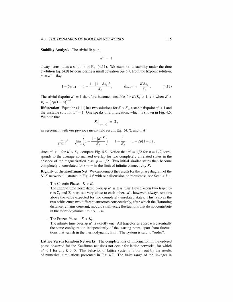
4.3. THE DYNAMICS OF BOOLEAN NETWORKS 115
Stability Analysis The trivial fixpoint
a∗ = 1
always constitutes a solution of Eq. (4.11). We examine its stability under the timeevolution Eq. (4.9) by considering a small deviation δat > 0 from the fixpoint solution,at = a∗−δat :
1−δat+1 = 1− 1− [1−δat ]K
Kc, δat+1 ≈
K δat
Kc. (4.12)
The trivial fixpoint a∗ = 1 therefore becomes unstable for K/Kc > 1, viz when K >
Kc =(2p(1− p)
)−1.
Bifurcation Equation (4.11) has two solutions for K >Kc, a stable fixpoint a∗ < 1 andthe unstable solution a∗ = 1. One speaks of a bifurcation, which is shown in Fig. 4.5.We note that
Kc
∣∣∣p=1/2
= 2 ,
in agreement with our previous mean-field result, Eq. (4.7), and that
limK→∞
a∗ = limK→∞
(1− 1− [a∗]K
Kc
)= 1− 1
Kc= 1−2p(1− p) ,
since a∗ < 1 for K > Kc, compare Fig. 4.5. Notice that a∗ = 1/2 for p = 1/2 corre-sponds to the average normalized overlap for two completely unrelated states in theabsence of the magnetization bias, p = 1/2. Two initial similar states then becomecompletely uncorrelated for t→ ∞ in the limit of infinite connectivity K.
Rigidity of the Kauffman Net We can connect the results for the phase diagram of theN–K network illustrated in Fig. 4.6 with our discussion on robustness, see Sect. 4.3.1.
– The Chaotic Phase: K > KcThe infinite time normalized overlap a∗ is less than 1 even when two trajecto-ries Σt and Σt start out very close to each other. a∗, however, always remainsabove the value expected for two completely unrelated states. This is so as thetwo orbits enter two different attractors consecutively, after which the Hammingdistance remains constant, modulo small-scale fluctuations that do not contributein the thermodynamic limit N→ ∞.
– The Frozen Phase: K < KcThe infinite time overlap a∗ is exactly one. All trajectories approach essentiallythe same configuration independently of the starting point, apart from fluctua-tions that vanish in the thermodynamic limit. The system is said to “order”.
Lattice Versus Random Networks The complete loss of information in the orderedphase observed for the Kauffman net does not occur for lattice networks, for whicha∗ < 1 for any K > 0. This behavior of lattice systems is born out by the resultsof numerical simulations presented in Fig. 4.7. The finite range of the linkages in
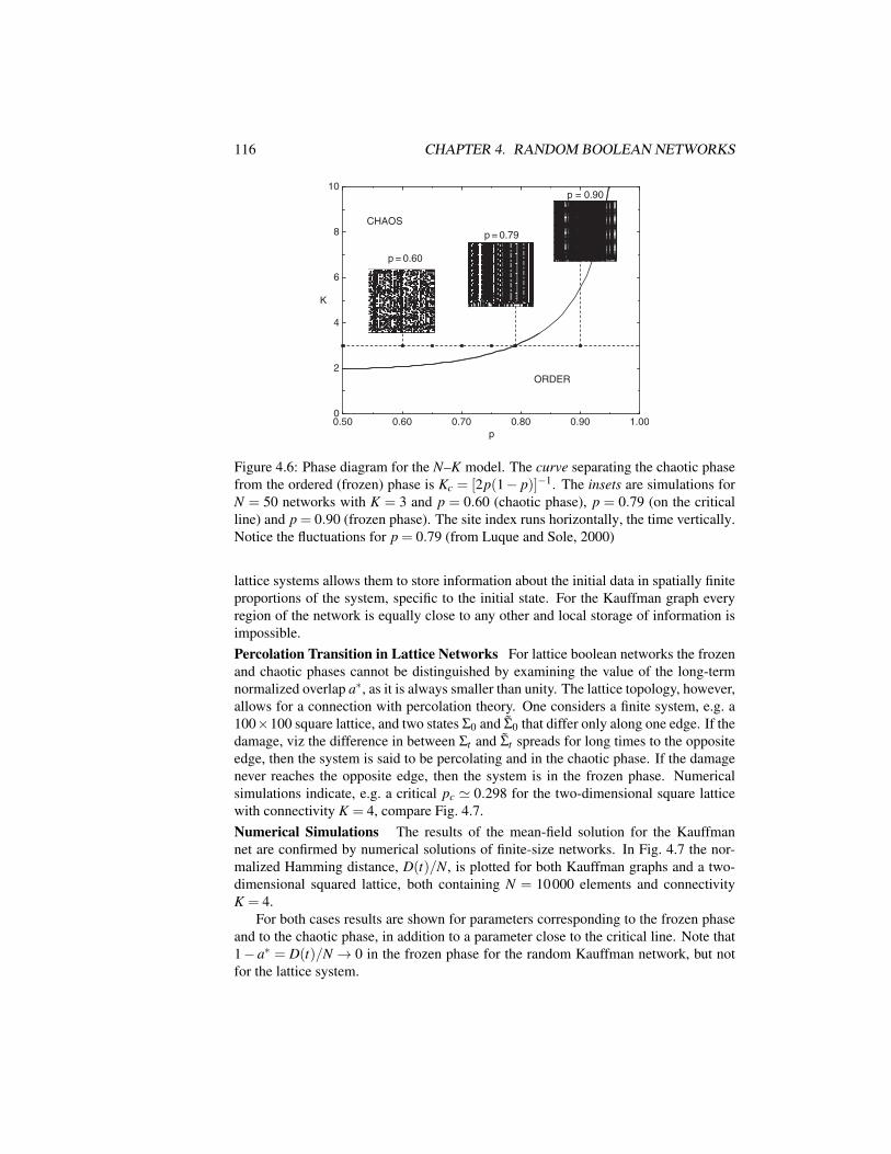
116 CHAPTER 4. RANDOM BOOLEAN NETWORKS
0.50 0.60 0.70 0.80 0.90 1.00
p
0
2
4
6
8
10
K
p = 0.60
p = 0.79
p = 0.90
CHAOS
ORDER
Figure 4.6: Phase diagram for the N–K model. The curve separating the chaotic phasefrom the ordered (frozen) phase is Kc = [2p(1− p)]−1. The insets are simulations forN = 50 networks with K = 3 and p = 0.60 (chaotic phase), p = 0.79 (on the criticalline) and p = 0.90 (frozen phase). The site index runs horizontally, the time vertically.Notice the fluctuations for p = 0.79 (from Luque and Sole, 2000)
lattice systems allows them to store information about the initial data in spatially finiteproportions of the system, specific to the initial state. For the Kauffman graph everyregion of the network is equally close to any other and local storage of information isimpossible.Percolation Transition in Lattice Networks For lattice boolean networks the frozenand chaotic phases cannot be distinguished by examining the value of the long-termnormalized overlap a∗, as it is always smaller than unity. The lattice topology, however,allows for a connection with percolation theory. One considers a finite system, e.g. a100×100 square lattice, and two states Σ0 and Σ0 that differ only along one edge. If thedamage, viz the difference in between Σt and Σt spreads for long times to the oppositeedge, then the system is said to be percolating and in the chaotic phase. If the damagenever reaches the opposite edge, then the system is in the frozen phase. Numericalsimulations indicate, e.g. a critical pc ' 0.298 for the two-dimensional square latticewith connectivity K = 4, compare Fig. 4.7.Numerical Simulations The results of the mean-field solution for the Kauffmannet are confirmed by numerical solutions of finite-size networks. In Fig. 4.7 the nor-malized Hamming distance, D(t)/N, is plotted for both Kauffman graphs and a two-dimensional squared lattice, both containing N = 10000 elements and connectivityK = 4.
For both cases results are shown for parameters corresponding to the frozen phaseand to the chaotic phase, in addition to a parameter close to the critical line. Note that1− a∗ = D(t)/N → 0 in the frozen phase for the random Kauffman network, but notfor the lattice system.

4.3. THE DYNAMICS OF BOOLEAN NETWORKS 117
0 100 200 300 400 500
t
0.007
0.008
0.009
0.010
D(t)/N
10−5
10−4
10−3
10−2
10−1
100
p = 0.4
pc= 0.15
p = 0.05
1 10 100 1000
t
D(t)/N
p = 0.4
pc = 0.27
p = 0.1
10−1
100
10−2
1 10 100 1000
pc= 0.1464
Figure 4.7: Normalized Hamming distance D(t)/N for a Kauffman net (left) and asquare lattice (right) with N = 10000 variables, connectivity K = 4 and D(0) = 100,viz D(0)/N = 0.01. Left: (top) Frozen phase (p = 0.05), critical (pc ' 0.1464) andchaotic (p = 0.4) phases, plotted with a logarithmic scale; (bottom) Hamming distancefor the critical phase (p = pc) but in a non-logarithmic graph. Right: Frozen phase(p = 0.1), critical (pc ' 0.27) and chaotic (p = 0.4) phases, plotted with a logarithmicscale. Note that a∗ = limt→∞(1−D(t)/N)< 1 in the frozen state of the lattice system,compare Fig. 4.5 (from Aldana et al., 2003)
4.3.4 Scale-Free Boolean Networks
The Kauffman model is a reference model which can be generalized in various ways,e.g. by considering small-world or scale-free networks.
Scale-Free Connectivity Distributions Scale-free connectivity distributions
P(K) =1
ζ (γ)K−γ , ζ (γ) =
∞
∑K=1
K−γ , γ > 1 (4.13)
abound in real-world networks, as discussed in Chap. 1. Here P(K) denotes the proba-bility to draw a coupling function fi(·) having Z arguments. The distribution Eq. (4.13)is normalizable for γ > 1.
The average connectivity 〈K〉 is
〈K〉 =∞
∑K=1
KP(K) =
∞ if 1< γ ≤ 2
ζ (γ−1)ζ (γ)
< ∞ if γ > 2, (4.14)
where ζ (γ) is the Riemann zeta function.
Annealed Approximation We consider again two states Σt and Σt and the normalizedoverlap
a(t) = 1−D(t)/N ,

118 CHAPTER 4. RANDOM BOOLEAN NETWORKS
which is identical to the probability that two vertices in Σ and Σ have the same value.In Sect. 4.3.3 we derived, for a magnetization bias p,
a(t +1) = 1− (1−ρK)2p(1− p) (4.15)
for the time-evolution of a(t), where
ρK = [a(t)]K →∞
∑K=1
[a(t)]K P(K) (4.16)
is the average probability that the K = 1,2, . . . controlling elements of the couplingfunction fi() are all identical. In Eq. (4.16) we have generalized Eq. (4.8) to a non-constant connectivity distribution P(K). We then find
a(t +1) = 1−2p(1− p)
1−
∞
∑K=1
aK(t)P(K)
≡ F(a(t)) , (4.17)
compare Eq. (4.9). Effectively we have used here an annealed model, due to the statis-tical averaging in Eq. (4.16).Fixpoints Within the Annealed Approximation In the limit t → ∞, Eq. (4.17) be-comes the self-consistency equation
a∗ = F(a∗) ,
for the fixpoint a∗, where F(a) is defined as the right-hand-side of Eq. (4.17). Again,a∗ = 1 is always a fixpoint of Eq. (4.17), since ∑K P(K) = 1 per definition.Stability of the Trivial Fixpoint We repeat the stability analysis of the trivial fixpointa∗ = 1 of Sect. 4.3.3 and assume a small deviation δa> 0 from a∗:
a∗−δa = F(a∗−δa) = F(a∗)−F ′(a∗)δa, δa = F ′(a∗)δa .
The fixpoint a∗ becomes unstable if F ′(a∗)> 1. We find for a∗ = 1
1 = lima→1−
dF(a)da
= 2p(1− p)∞
∑k=1
KP(K)
= 2p(1− p)〈K〉 . (4.18)
For lima→1− dF(a)/da < 1 the fixpoint a∗ = 1 is stable, otherwise it is unstable. Thephase transition is then given by
2p(1− p)〈K〉 = 1 . (4.19)
For the classical N–K model all elements have the same connectivity, Ki = 〈K〉 = K,and Eq. (4.19) reduces to Eq. (4.12).The Frozen and Chaotic Phases for the Scale-Free Model For 1< γ ≤ 2 the averageconnectivity is infinite, see Eq. (4.14). F ′(1) = 2p(1− p) 〈K〉 is then always larger thanunity and a∗ = 1 unstable, as illustrated in Fig. 4.8. Equation (4.17) then has a stablefixpoint a∗ 6= 1; the system is in the chaotic phase for all p ∈]0,1[.

4.4. CYCLES AND ATTRACTORS 119
1 1.5 2.5 3
γ
0
0.2
0.4
0.6
0.8
1
pChaotic Phase
Ordered
Phase
2
Figure 4.8: Phase diagram for a scale-free boolean network with connectivity distribu-tion ∝ K−γ . The average connectivity diverges for γ < 2 and the network is chaotic forall p (from Aldana and Cluzel, 2003)
For γ > 2 the first moment of the connectivity distribution P(K) is finite and thephase diagram is identical to that of the N–K model shown in Fig. 4.6, with K replacedby ζ (γc−1)/ζ (γc). The phase diagram in γ–p space is presented in Fig. 4.8. One findsthat γc ∈ [2,2.5] for any value of p. There is no chaotic scale-free network for γ > 2.5.It is interesting to note that γ ∈ [2,3] for many real-world scale-free networks.
4.4 Cycles and AttractorsWe have emphasized so far the general properties of boolean networks, such as thephase diagram. We now turn to a more detailed inspection of the dynamics, particularyregarding the structure of the attractors.
4.4.1 Quenched Boolean Dynamics
Self-Retracting Orbits From now on we consider quenched systems for whichthe coupling functions fi(σi1 , . . . ,σiK ) are fixed for all times. Any orbit eventuallypartly retraces itself, since the state space Ω = 2N is finite. The long-term trajectory istherefore cyclic.
Attractors. An attractor A0 of a discrete dynamical system is a regionΣt ⊂ Ω in phase space that maps completely onto itself under the timeevolution At+1 = At ≡ A0.
Attractors are typically cycles
Σ(1) → Σ
(2) → . . . → Σ(1) ,

120 CHAPTER 4. RANDOM BOOLEAN NETWORKS
σ2
σ12
σ11 σ14
σ1 σ17
σ3 σ1
σ5 σ18
σ6 σ1
σ7 σ17
σ8 σ18
σ9 σ13
σ10 σ15
σ12 σ11
σ13 σ16
σ15 σ7
σ16 σ19
σ17 σ16
σ18 σ7
σ19 σ15
σ20 σ10
σ2σ2
σ4 σ18
σ11 σ11
σ14 σ11
σ16
σ17
σ7
σ15
σ18 σ5
σ4
σ13
σ1
σ9
σ20
σ8σ19
σ3σ6
σ10
Figure 4.9: Cycles and linkages. Left: Sketch of the state space where every boldpoint stands for a state Σt = σ1, . . . ,σN. The state space decomposes into distinctattractor basins for each cycle attractor or fixpoint attractor. Right: Linkage loops foran N = 20 model with K = 1. The controlling elements are listed in the center column.Each arrow points from the controlling element toward the direct descendant. Thereare three modules of uncoupled variables (from Aldana et al., 2003)
see Figs. 4.3 and 4.9 for some examples. Fixed points are cycles of length 1.
The Attraction Basin. The attraction basin B of an attractor A0 is theset Σt ⊂Ω for which there is a time T < ∞ such that ΣT ∈ A0.
The probability to end up in a given cycle is directly proportional, for randomly drawninitial conditions, to the size of its basin of attraction. The three-site network illustratedin Fig. 4.3 is dominated by the fixpoint 1,1,1, which is reached with probability 5/8for random initial starting states.Attractors are Everywhere Attractors and fixpoints are generic features of dynami-cal systems and are very important for their characterization, as they dominate the timeevolution in state space within their respective basins of attraction. Random booleannetworks allow for very detailed studies of the structure of attractors and of the connec-tion to network topology. Of special interest in this context is how various propertiesof the attractors, like the cycle length and the size of the attractor basins, relate to thethermodynamic differences between the frozen phase and the chaotic phase. These arethe issues that we shall now discuss.Linkage Loops, Ancestors and Descendants Every variable σi can appear as anargument in the coupling functions for other elements; it is said to act as a controllingelement. The collections of all such linkages can be represented graphically by a di-rected graph, as illustrated in Figs. 4.1, 4.3 and 4.9, with the vertices representing theindividual binary variables. Any given element σi can then influence a large number ofdifferent states during the continued time evolution.
Ancestors and Descendants. The elements a vertex affects con-secutively via the coupling functions are called its descendants. Goingbackwards in time one find ancestors for each element.

4.4. CYCLES AND ATTRACTORS 121
In the 20-site network illustrated in Fig. 4.9 the descendants of σ11 are σ11, σ12 andσ14.
When an element is its own descendant (and ancestor) it is said to be part of a“linkage loop”. Different linkage loops can overlap, as is the case for the linkage loops
σ1→ σ2→ σ3→ σ4→ σ1, σ1→ σ2→ σ3→ σ1
shown in Fig. 4.1. Linkage loops are disjoint for K = 1, compare Fig. 4.9.
Modules and Time Evolution The set of ancestors and descendants determines theoverall dynamical dependencies.
Module. The collection of all ancestors and descendants of a givenelement σi is called the module (or component) to which σi belongs.
If we go through all variables σi, i = 1, . . . ,N we find all modules, with every elementbelonging to one and only one specific module. Otherwise stated, disjoint modules cor-respond to disjoint subgraphs, the set of all modules constitute the full linkage graph.The time evolution is block-diagonal in terms of modules; σi(t) is independent of allvariables not belonging to its own module, for all times t.
In lattice networks the clustering coefficient (see Chap. 1) is large and closed link-age loops occur frequently. For big lattice systems with a small mean linkage K weexpect far away spatial regions to evolve independently, due the lack of long-rangeconnections.
Relevant Nodes and Dynamic Core Taking a look at dynamics of the 20-site modelillustrated in Fig. 4.9, we notice that, e.g., the elements σ12 and σ14 just follow the dy-namics of σ11, they are “enslaved” by σ11. These two elements do not control any otherelement and one could just delete them from the system wihout qualitative changes tothe overall dynamics.
Relevant Nodes. A node is termed relevant if its state is not constantand if it controls at least one other relevant element (eventually itself).
An element is constant if it evolves, indepedently of the initial conditions, always tothe same state and not constant otherwise. The set of relevant nodes, the dynamic core,controls the overall dynamics. The dynamics of all other nodes can be disregardedwithout changing the attractor structure. The node σ13 of the 20-site network illustratedin Fig. 4.9 is relevant if the boolean function connecting it to itself is either the identityor the negation (see p. 108).
The concept of a dynamic core is of great importance for practical applications.Gene expression networks may be composed of thousands of nodes, but contain gener-ally a relatively small dynamic core controlling the overall network dynamics. This isthe case, e.g., for the gene regulation network controlling the yeast cell cycle discussedin Sect. 4.5.2.
Lattice Nets versus Kauffman Nets For lattice systems the linkages are short-rangedand whenever a given element σ j acts as a controlling element for another element σithere is a high probability that the reverse is also true, viz that σi is an argument of f j.

122 CHAPTER 4. RANDOM BOOLEAN NETWORKS
The linkages are generally non-reciprocal for the Kauffman net; the probability forreciprocality is just K/N and vanishes in the thermodynamic limit for finite K. Thenumber of disjoint modules in a random network therefore grows more slowly thanthe system size. For lattice systems, on the other hand, the number of modules isproportional to the size of the system. The differences between lattice and Kauffmannetworks translate to different cycle structures, as every periodic orbit for the full sys-tem is constructed out of the individual attractors of all modules present in the networkconsidered.
4.4.2 The K = 1 Kauffman Network
We start our discussion of the cycle structure of Kauffman nets with the case K = 1,which can be solved exactly. The maximal length for a linkage loop lmax is on theaverage of the order of
lmax ∼ N1/2 . (4.20)
The linkage loops determine the cycle structure together with the choice of the couplingensemble. As an example we discuss the case of an N = 3 linkage loop.
The Three-site Linkage Loop with Identities For K = 1 there are only two non-constant coupling functions, i.e. the identity I and the negation ¬, see p. 108. We startby considering the case of all the coupling functions being the identity:
ABC → CAB → BCA → ABC → . . . ,
where we have denoted by A,B,C the values of the binary variables σi, i= 1,2,3. Thereare two cycles of length 1, in which all elements are identical. When the three elementsare not identical, the cycle length is 3. The complete dynamics is then:
000 → 000111 → 111
100 → 010 → 001 → 100011 → 101 → 110 → 011
Three-Site Linkage Loops with Negations Let us consider now the case that allthree coupling functions are negations:
ABC → CAB → BCA → ABC → . . . A = ¬A, etc. .
The cycle length is 2 if all elements are identical
000 → 111 → 000
and of length 6 if they are not.
100 → 101 → 001 → 011 → 010 → 110 → 100 .
The complete state space Ω = 23 = 8 decomposes into two cycles, one of length 6 andone of length 2.

4.4. CYCLES AND ATTRACTORS 123
Three-Site Linkage Loops with a Constant Function Let us see what happens if anyof the coupling functions are a constant function. For illustration purposes we considerthe case of two constant functions 0 and 1 and the identity:
ABC → 0A1 → 001 → 001 . (4.21)
Generally it holds that the cycle length is 1 if any of the coupling functions is anidentity and that there is then only a single fixpoint attractor. Equation (4.21) holds forall A,B,C ∈ 0,1; the basin of attraction for 001 is therefore the whole state space,and 001 is a global attractor.
The Kauffman net can contain very large linkage loops for K = 1, see Eq. (4.20),but then the probability that a given linkage loop contains at least one constant functionis also very high. The average cycle length therefore remains short for the K = 1Kauffman net.
Loops and Attractors The attractors are made up of the set of linkage loops. As anexample we consider a 5-site network with two linkage loops,
A →I B →I C →I A, D →I E →I D ,
with all coupling functions being the identity I. The states
00000, 00011, 11100, 11111
are fixpoints in phase space Σ = ABCDE. Examples of cyclic attrators of length 3 and6 are
10000 → 01000 → 00100 → 10000
and
10010 → 01001 → 00110 → 10001 → 01010 → 00101 → 10010 .
In general, the length of an attractor is given by the least common multiple of theperiods of the constituent loops. This relation holds for K = 1 Boolean networks, forgeneral K the attractors are composed of the cycles of the constituent set of modules.
Critical K = 1 Boolean networks When the coupling ensemble is selected uniformly,compare Sect. 4.2.2, the K = 1 network is in the frozen state. If we do however restrictour coupling ensemble to the identity I and to the negation ¬, the value of one nodeis just copied or inverted to exactly one other node. There is no loss of informationanymore, when disregarding the two constant K = 1 coupling functions (see p. 108).The information is not multiplied either, being transmitted to exactly one and not morenodes. The network is hence critical, as pointed out in Sect. 4.3.1.
4.4.3 The K = 2 Kauffman NetworkThe K = 2 Kauffman net is critical, as discussed in Sects. 4.3.1 and 4.3.2. When phys-ical systems undergo a (second-order) phase transition, power laws are expected rightat the point of transition for many response functions; see the discussion in Chap. 2. It

124 CHAPTER 4. RANDOM BOOLEAN NETWORKS
is therefore natural to expect the same for critical dynamical systems, such as a randomboolean network.
This expectation was indeed initially born out of a series of mostly numerical in-vestigations, which indicated that both the typical cycle lengths, as well as the meannumber of different attractors, would grow algebraically with N, namely like
√N. It
was therefore tempting to relate many of the power laws seen in natural organisms tothe behavior of critical random boolean networks.Undersampling of the State Space The problem to determine the number and thelength of cycles is, however, numerically very difficult. In order to extract power lawsone has to simulate systems with large N. The state space Ω = 2N , however, growsexponentially, so that an exhaustive enumeration of all cycles is impossible. One hastherefore to resort to a weighted sampling of the state space for any given network re-alization and to extrapolate from the small fraction of states sampled to the full statespace. This method yielded the
√N dependence referred to above.
The weighted sampling is, however, not without problems; it might in principleundersample the state space. The number of cycles found in the average state spacemight not be representative for the overall number of cycles, as there might be smallfractions of state space with very high number of attractors dominating the total numberof attractors.
This is indeed the case. One can prove rigorously that the number of attractorsgrows faster than any power for the K = 2 Kauffman net. One might still argue, how-ever, that for biological applications the result for the “average state space” is relevant,as biological systems are not too big anyway. The hormone regulation network ofmammals contains of the order of 100 elements, the gene regulation network of theorder of 20 000 elements.
4.4.4 The K = N Kauffman NetworkMean-field theory holds for the fully connected network K = N and we can evaluatethe average number and length of cycles using probability arguments.The Random Walk Through Configuration Space We consider an orbit startingfrom an arbitrary configuration Σ0 at time t = 0. The time evolution generates a seriesof states
Σ0, Σ1, Σ2, . . .
through the configuration space of size Ω = 2N . We consider all Σt to be uncorrelated,viz we consider a random walk. This assumption holds due to the large connectivityK = N.Closing the Random Walk The walk through configuration space continues until wehit a previously visited point, see Fig. 4.10. We define by
– qt : the probability that the trajectory remains unclosed after t steps;
– Pt : the probability of terminating the excursion exactly at time t.
If the trajectory is still open at time t, we have already visited t + 1 different sites(including the sites Σ0 and Σt ). Therefore, there are t +1 ways of terminating the walk

4.4. CYCLES AND ATTRACTORS 125
Σ 0 Σ 1
1−ρt
ρt
Σ 2 Σ 3 Σ t Σ t+1
Σ t+1
Figure 4.10: A random walk in configuration space. The relative probability of closingthe loop at time t, ρt = (t + 1)/Ω, is the probability that Σt+1 ≡ Σt ′ , with a certaint ′ ∈ [0, t]
at the next time step. The relative probability of termination is then ρt = (t +1)/Ω andthe overall probability Pt+1 to terminate the random walk at time t +1 is
Pt+1 = ρt qt =t +1
Ωqt .
The probability of still having an open trajectory after t +1 steps is
qt+1 = qt(1−ρt) = qt
(1− t +1
Ω
)= q0
t+1
∏i=1
(1− i
Ω
), q0 = 1 .
The phase space Ω = 2N diverges in the thermodynamic limit N→ ∞ and the approxi-mation
qt =t
∏i=1
(1− i
Ω
)≈
t
∏i=1
e−i/Ω = e−∑i i/Ω = e−t(t+1)/(2Ω) (4.22)
becomes exact in this limit. For large times t we have t(t + 1)/(2Ω) ≈ t2/(2Ω) inEq. (4.22). The probability
Ω
∑t=1
Pt '∫
∞
0dt
tΩ
e−t2/(2Ω) = 1
for the random walk to close at all is unity.Cycle Length Distribution The probability 〈Nc(L)〉 that the system contains a cycleof length L is
〈Nc(L)〉 =qt=L
Ω
Ω
L=
exp[−L2/(2Ω)]
L, (4.23)
where we used Eq. (4.22). 〈· · ·〉 denotes an ensemble average over realizations. Inderiving Eq. (4.23) we used the following considerations:
(i) The probability that Σt+1 is identical to Σ0 is 1/Ω.
(ii) There are Ω possible starting points (factor Ω).
(iii) Factor 1/L corrects for the overcounting of cycles when considering the L pos-sible starting sites of the L-cycle.

126 CHAPTER 4. RANDOM BOOLEAN NETWORKS
Average Number of Cycles We are interested in the mean number Nc of cycles,
Nc =N
∑L=1〈Nc(L)〉 '
∫∞
1dL〈Nc(L)〉 . (4.24)
When going from the sum ∑L to the integral∫
dL in Eq. (4.24) we neglected terms oforder unity. We find
Nc =∫
∞
1dL
exp[−L2/(2Ω)]
L=∫ 1
1/√
2Ω
due−u2
u︸ ︷︷ ︸≡ I1
+∫
∞
1du
e−u2
u︸ ︷︷ ︸≡ I2
,
where we rescaled the variable by u=L/√
2Ω. For the separation∫
∞
1/√
2Ω=∫ c
1/√
2Ω+∫
∞
cof the integral above we used c = 1 for simplicity; any other finite value for c would doalso the job.
The second integral, I2, does not diverge as Ω→ ∞. For I1 we have
I1 =∫ 1
1/√
2Ω
due−u2
u=∫ 1
1/√
2Ω
du1u
(1−u2 +
12
u4 + . . .)
≈ ln(√
2Ω) , (4.25)
since all further terms ∝∫ 1
1/√
2Ωduun−1 <∞ for n = 2,4, . . . and Ω→∞. The aver- age
number of cycles is then
Nc = ln(√
2N) + O(1) =N ln2
2+ O(1) (4.26)
for the N = K Kauffman net in thermodynamic limit N→ ∞.Mean Cycle Length The average length L of a random cycle is
L =1
Nc
∞
∑L=1
L〈Nc(L)〉 ≈1
Nc
∫∞
1dLL
exp[−L2/(2Ω)]
L
=1
Nc
∫∞
1dL e−L2/(2Ω) =
√2Ω
Nc
∫∞
1/√
2Ω
du e−u2(4.27)
after rescaling with u=L/√
2Ω and using Eq. (4.23). The last integral on the right-hand-sideof Eq. (4.27) converges for Ω→∞ and the mean cycle length L consequently scales as
L ∼ Ω1/2/N = 2N/2/N (4.28)
for the K = N Kauffman net, when using Eq. (4.24), Nc ∼ N.
4.5 Applications
4.5.1 Living at the Edge of Chaos
Gene Expression Networks and Cell Differentiation Kauffman introduced the N–Kmodel in the late 1960s for the purpose of modeling the dynamics and time evolution

4.5. APPLICATIONS 127
of networks of interacting genes, i.e. the gene expression network. In this model anactive gene might influence the expression of any other gene, e.g. when the proteintranscripted from the first gene influences the expression of the second gene.
The gene expression network of real-world cells is not random. The web of linkagesand connectivities among the genes in a living organism is, however, very intricate,and to model the gene–gene interactions as randomly linked is a good zero-th orderapproximation. One might then expect to gain a generic insight into the properties ofgene expression networks; insights that are independent of the particular set of linkagesand connectivities realized in any particular living cell.
Dynamical Cell Differentiation Whether random or not, the gene expression net-work needs to result in a stable dynamics in order for the cell to keep functioning.Humans have only a few hundreds of different cell types in their bodies. Consideringthe fact that every single cell contains the identical complete genetic material, in 1969Kauffman proposed an, at that time revolutionary, suggestion that every cell type cor-responds to a distinct dynamical state of the gene expression network. It is natural toassume that these states correspond to attractors, viz in general to cycles. The averagelength L of a cycle in a N–K Kauffman net is
L ∼ 2αN
in the chaotic phase, e.g. for N = K where α = 1/2, see Eq. (4.28), The mean cy-cle length L is exponentially large; consider that N ≈ 20000 for the human genome.A single cell would take the universe’s lifetime to complete a single cycle, which isan unlikely setting. It then follows that gene expression networks of living organismscannot be operational in the chaotic phase.
Living at the Edge of Chaos If the gene expression network cannot operate in thechaotic phase there are but two possibilities left: the frozen phase or the critical point.The average cycle length is short in the frozen phase, see Sect. 4.4.2, and the dynamicsstable. The system is consequently very resistant to damage of the linkages.
But what about Darwinian evolution? Is too much stability good for the adapt-ability of cells in a changing environment? Kauffman suggested that gene expressionnetworks operate at the edge of chaos, an expression that has become legendary. Bythis he meant that networks close to criticality may benefit from the stability propertiesof the close-by frozen phase and at the same time exhibit enough sensitivity to changesin the network structure so that Darwinian adaption remains possible.
But how can a system reach criticality by itself? For the N–K network there is noextended critical phase, only a single critical point K = 2. In Chap. 5 we will discussmechanisms that allow certain adaptive systems to evolve their own internal parametersautonomously in such a way that they approach the critical point. This phenomenon iscalled “self-organized criticality”.
One could then assume that Darwinian evolution trims the gene expression net-works towards criticality: Cells in the chaotic phase are unstable and die; cells deepin the frozen phase cannot adapt to environmental changes and are selected out in thecourse of time.
128 CHAPTER 4. RANDOM BOOLEAN NETWORKS
Cell Size
Cln3
MBF
Clb5,6
Mcm1/SFF
Swi5 Cdc20&Cdc14
Cdh1
Cln1,2
SBF
Sic1
Clb1,2
Figure 4.11: The N = 11 core network responsible for the yeast cell cycle. Acronymsdenote protein names, solid arrows excitatory connections and dashed arrows in-hibitory connections. Cln3 is inactive in the resting state G1 and becomes active whenthe cell reaches a certain size (top), initiating the cell division process (compare Li etal., 2004)
4.5.2 The Yeast Cell Cycle
The Cell Division Process Cells have two tasks: to survive and to multiply. When aliving cell grows too big, a cell division process starts. The cell cycle has been studiedintensively for the budding yeast. In the course of the division process the cell goesthrough a distinct set of states
G1 → S → G2 → M → G1 ,
with G1 being the “ground state” in physics slang, viz the normal cell state and thechromosome division takes place during the M phase. These states are characterizedby distinct gene activities, i.e. by the kinds of proteins active in the cell. All eukaryotecells have similar cell division cycles.
The Yeast Gene Expression Network From the ≈ 800 genes involved only 11–13core genes are actually regulating the part of the gene expression network responsiblefor the division process; all other genes are more or less just descendants of the coregenes. The cell dynamics contains certain checkpoints, where the cell division processcan be stopped if something were to go wrong. When eliminating the checkpoints acore network with only 11 elements remains. This network is shown in Fig. 4.11.
Boolean Dynamics The full dynamical dependencies are not yet known for the yeastgene expression network. The simplest model is to assume
σi(t) =
1 if ai(t)> 00 if ai(t)≤ 0 , ai(t) = ∑
jwi jσ j(t) , (4.29)

4.5. APPLICATIONS 129
Figure 4.12: The yeast cell cycle as an attractor trajectory of the gene expression net-work. Shown are the 1764 states (green dots, out of the 211 = 2048 states in phasespace Ω) making up the basin of attraction of the biologically stable G1 state (at thebottom). After starting with the excited G1 normal state (the first state in the biolog-ical pathway represented by blue arrows), compare Fig. 4.11, the boolean dynamicsruns through the known intermediate states (blue arrows) until the G1 states attractor isagain reached, representing the two daughter cells (from Li et al., 2004)
i.e. a boolean dynamics4 for the binary variables σi(t) = 0,1 representing the acti-vation/deactivation of protein i, with couplings wi j = ±1 for an excitatory/inhibitoryfunctional relation.Fixpoints The 11-site network has 7 attractors, all cycles of length 1, viz fixpoints.The dominating fixpoint has an attractor basin of 1764 states, representing about 72%of the state space Ω = 211 = 2048. Remarkably, the protein activation pattern of thedominant fixpoint corresponds exactly to that of the experimentally determined G1ground state of the living yeast cell.The Cell Division Cycle In the G1 ground state the protein Cln3 is inactive. Whenthe cell reaches a certain size it becomes expressed, i.e. it becomes active. For thenetwork model one then just starts the dynamics by setting
σCln3 → 1, at t = 0
in the G1 state. The ensuing simple boolean dynamics, induced by Eq. (4.29), is de-picted in Fig. 4.12.
The remarkable result is that the system follows an attractor pathway that runsthrough all experimentally known intermediate cell states, reaching the ground stateG1 in 12 steps.
4Genes are boolean variables in the sense that they are either expressed or not. The quantitative amountof proteins produced by a given active gene is regulated via a separate mechanism involving microRNA,small RNA snippets.

130 CHAPTER 4. RANDOM BOOLEAN NETWORKS
Ensembles of neurons
Random boolean network
with cycles and attractors
t
t
Time−dependent output−
cycles depend on input
Figure 4.13: Illustration of ensemble (a) and time (b) encoding. Left: All receptorneurons corresponding to the same class of input signals are combined, as occurs inthe nose for different odors. Right: The primary input signals are mixed together by arandom neural network close to criticality and the relative weights are time encoded bythe output signal
Comparison with Random Networks The properties of the boolean network de-picted in Fig. 4.11 can be compared with those of a random boolean network. A ran-dom network of the same size and average connectivity would have more attractorswith correspondingly smaller basins of attraction. Living cells clearly need a robustprotein network to survive in harsh environments.
Nevertheless, the yeast protein network shows more or less the same susceptibilityto damage as a random network. The core yeast protein network has an average con-nectivity of 〈K〉= 27/11' 2.46. The core network has only N = 11 sites, a number fartoo small to allow comparison with the properties of N–K networks in the thermody-namic limit N→ ∞. Nevertheless, an average connectivity of 2.46 is remarkably closeto K = 2, i.e. the critical connectivity for N–K networks.Life as an Adaptive Network Living beings are complex and adaptive dynamicalsystems; a subject that we will further dwell on in Chap. 6. The here discussed prelim-inary results on the yeast gene expression network indicate that this statement is notjust an abstract notion. Adaptive regulative networks constitute the core of all living.
4.5.3 Application to Neural Networks
Time Encoding by Random Neural Networks There is some debate in neurosciencewhether, and to which extent, time encoding is used in neural processing.
– Ensemble Encoding: Ensemble encoding is present when the activity of a sen-sory input is transmitted via the firing of certain ensembles of neurons. Everysensory input, e.g. every different smell sensed by the nose, has its respectiveneural ensemble.
– Time Encoding: Time encoding is present if the same neurons transmit more thanone piece of sensory information by changing their respective firing patterns.
Cyclic attractors in a dynamical ensemble are an obvious tool to generate time encodedinformation. For random boolean networks as well as for random neural networks ap-
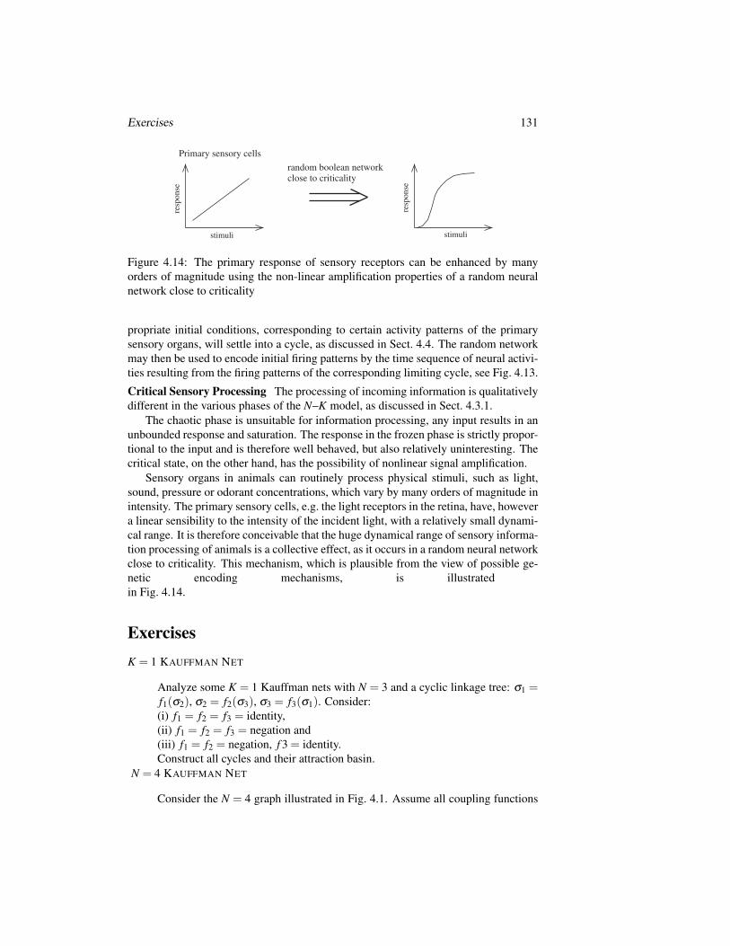
Exercises 131
resp
onse
stimuli
resp
onse
stimuli
Primary sensory cells
random boolean networkclose to criticality
Figure 4.14: The primary response of sensory receptors can be enhanced by manyorders of magnitude using the non-linear amplification properties of a random neuralnetwork close to criticality
propriate initial conditions, corresponding to certain activity patterns of the primarysensory organs, will settle into a cycle, as discussed in Sect. 4.4. The random networkmay then be used to encode initial firing patterns by the time sequence of neural activi-ties resulting from the firing patterns of the corresponding limiting cycle, see Fig. 4.13.
Critical Sensory Processing The processing of incoming information is qualitativelydifferent in the various phases of the N–K model, as discussed in Sect. 4.3.1.
The chaotic phase is unsuitable for information processing, any input results in anunbounded response and saturation. The response in the frozen phase is strictly propor-tional to the input and is therefore well behaved, but also relatively uninteresting. Thecritical state, on the other hand, has the possibility of nonlinear signal amplification.
Sensory organs in animals can routinely process physical stimuli, such as light,sound, pressure or odorant concentrations, which vary by many orders of magnitude inintensity. The primary sensory cells, e.g. the light receptors in the retina, have, howevera linear sensibility to the intensity of the incident light, with a relatively small dynami-cal range. It is therefore conceivable that the huge dynamical range of sensory informa-tion processing of animals is a collective effect, as it occurs in a random neural networkclose to criticality. This mechanism, which is plausible from the view of possible ge-netic encoding mechanisms, is illustratedin Fig. 4.14.
ExercisesK = 1 KAUFFMAN NET
Analyze some K = 1 Kauffman nets with N = 3 and a cyclic linkage tree: σ1 =f1(σ2), σ2 = f2(σ3), σ3 = f3(σ1). Consider:(i) f1 = f2 = f3 = identity,(ii) f1 = f2 = f3 = negation and(iii) f1 = f2 = negation, f 3 = identity.Construct all cycles and their attraction basin.
N = 4 KAUFFMAN NET
Consider the N = 4 graph illustrated in Fig. 4.1. Assume all coupling functions

132 CHAPTER 4. RANDOM BOOLEAN NETWORKS
to be generalized XOR-functions (1/0 if the number of input-1’s is odd/even).Find all cycles.
SYNCHRONOUS VS. ASYNCHRONOUS UPDATING
Consider the dynamics of the three-site network illustrated in Fig. 4.3 undersequential asynchronous updating. At every time step first update σ1 then σ2and then σ3. Determine the full network dynamics, find all cycles and fixpointsand compare with the results for synchronous updating shown in Fig. 4.3.
LOOPS AND ATTRACTORS
Consider, as in Sect. 4.4.2, a K = 1 network with two linkage loops,
A →I B →¬ C →I A, D →¬ E →¬ D ,
with I denoting the identity coupling and ¬ the negation, compare p. 108. Findall attractors by considering first the dynamics of the individual linkage loops. Isthere any state in phase space which is not part of any cycle?
RELEVANT NODES AND DYNAMIC CORE
How many constant nodes does the network shown in Fig. 4.3 have? Replacethen the AND function with XOR and calculated the complete dynamics. Howmany relevant nodes are there now?
THE HUEPE AND ALDANA NETWORK
Solve the boolean neural network with uniform coupling functions and noise,
σi(t +1) =
sign
(∑
Kj=1 σi j(t)
)with probability 1−η ,
−sign(
∑Kj=1 σi j(t)
)with probability η ,
via mean-field theory, where σi =±1, by considering the order parameter
Ψ = limT→∞
1T
∫ T
0|s(t)|dt, s(t) = lim
N→∞
1N
N
∑i=1
σi(t) .
See Huepe and Aldana-Gonzalez (2002) and additional hints in the solutionssection.
BOND PERCOLATION
Consider a finite L×L two-dimensional square lattice. Write a code that gen-erates a graph by adding with probability p ∈ [0,1] nearest-neighbor edges. Tryto develop an algorithm searching for a non-interrupted path of bonds from oneedge to the opposite edge; you might consult web resources. Try to determinethe critical pc, for p > pc, a percolating path should be present with probability1 for very large systems L.

Further Reading 133
Further Reading
The interested reader may want to take a look at Kauffman’s (1969) seminal work onrandom boolean networks, or to study his book (Kauffman, 1993). For reviews onboolean networks please consult Aldana, Coppersmith and Kadanoff (2003) and thecorresponding chapter by B. Drossel in Schuster (2008).
Examples of additional applications of boolean network theory regarding the mod-eling of neural networks (Wang et al., 1990) and of evolution (Bornholdt and Sneppen,1998) are also recommended. Some further interesting original literature concerns theconnection of Kauffman nets with percolation theory (Lam, 1988), as well as the exactsolution of the Kauffman net with connectivity one (Flyvbjerg and Kjaer, 1988), nu-merical studies of the Kauffman net (Flyvbjerg, 1989; Kauffman, 1969, 1990; Bastollaand Parisi, 1998), as well as the modeling of the yeast reproduction cycle by booleannetworks (Li et al., 2004).
Some of the new developments concern the stability of the Kauffman net (Bilke andSjunnesson, 2001) and the number of attractors (Samuelsson and Troein, 2003) andapplications to time encoding by the cyclic attractors (Huerta and Rabinovich, 2004)and nonlinear signal amplification close to criticality (Kinouchi and Copelli, 2006).
ALDANA-GONZALEZ, M., CLUZEL, P. 2003 A natural class of robust networks. Proceedingsof the National Academy of Sciences 100, 8710–8714.
ALDANA-GONZALEZ, M., COPPERSMITH, S., KADANOFF, L.P. 2003 Boolean dynamicswith random couplings. In Kaplan, E., Marsden, J.E., Sreenivasan, K.R. (eds.) Perspectivesand Problems in Nonlinear Science. A Celebratory Volume in Honor of Lawrence Sirovich,pp. 23–89. Springer Applied Mathematical Sciences Series, Berlin.
BASTOLLA, U., PARISI, G. 1998 Relevant elements, magnetization and dynamical propertiesin Kauffman networks: A numerical study. Physica D 115, 203–218.
BILKE, S., SJUNNESSON, F. 2001 Stability of the Kauffman model. Physical Review E 65,016129.
BORNHOLDT, S., SNEPPEN, K. 1998 Neutral mutations and punctuated equilibrium in evolv-ing genetic networks. Physical Review Letters 81, 236–239.
FLYVBJERG, H. 1989 Recent results for random networks of automata. Acta Physica PolonicaB 20, 321–349.
FLYVBJERG, H., KJAER, N.J. 1988 Exact solution of Kauffman model with connectivityone. Journal of Physics A: Mathematical and General 21, 1695–1718.
HUEPE, C., ALDANA-GONZALEZ, M. 2002 Dynamical phase transition in a neural networkmodel with noise: An exact solution. Journal of Statistical Physics 108, 527–540.
HUERTA, R., RABINOVICH, M. 2004 Reproducible sequence generation in random neuralensembles. Physical Review Letters 93, 238104.
KAUFFMAN, S. A. 1969 Metabolic stability and epigenesis in randomly constructed nets.Journal of Theoretical Biology 22, 437–467.
KAUFFMAN, S.A. 1990 Requirements for evolvability in complex systems – orderly dynam-ics and frozen components. Physica D 42, 135–152.
KAUFFMAN, S.A. 1993 The Origins of Order: Self-Organization and Selection in Evolution.Oxford University Press, New York.
134 4 Random Boolean Networks
KINOUCHI, O., COPELLI, M. 2006 Optimal dynamical range of excitable networks at criti-cality. Nature Physics 2, 348–352.
LAM, P.M. 1988 A percolation approach to the Kauffman model. Journal of StatisticalPhysics 50, 1263–1269.
LI, F., LONG, T., LU, Y., OUYANG, Q., TANG, C. 2004 The yeast cell-cycle network isrobustly designed. Proceedings of the National Academy Science 101, 4781–4786.
LUQUE, B., SOLE, R.V. 2000 Lyapunov exponents in random boolean networks. Physica A284, 33–45.
SAMUELSSON, B., TROEIN, C. 2003 Superpolynomial growth in the number of attractors inKauffman networks. Physical Review Letters 90, 098701.
SCHUSTER, H.G. (EDITOR) 2008 Reviews of Nonlinear Dynamics and Complexity: Volume1. Wiley-VCH, New York.
SOMOGYI, R., SNIEGOSKI, C.A. 1996 Modeling the complexity of genetic networks: Un-derstanding multigenetic and pleiotropic regulation. Complexity 1, 45–63.
WANG, L., PICHLER, E.E., ROSS, J. 1990 Oscillations and chaos in neural networks – anexactly solvable model. Proceedings of the National Academy of Sciences of the UnitedStates of America 87, 9467–9471.

Further Reading 135
Table 4.1: Examples of boolean functions of three arguments. (a) A particu-lar random function. (b) A canalizing function of the first argument. Whenσ1 = 0, the function value is 1. If σ1 = 1, then the output can be either 0or 1. (c) An additive function. The output is 1 (active) if at least two in-puts are active. (d) The generalized XOR, which is true when the number of1-bits is odd
σ1 σ2 σ3 f (σ1,σ2,σ3)
Random Canalizing Additive Gen. XOR
0 0 0 0 1 0 00 0 1 1 1 0 10 1 0 1 1 0 10 1 1 0 1 1 01 0 0 1 0 0 11 0 1 0 1 1 01 1 0 1 0 1 01 1 1 1 0 1 1
Table 4.2: The 16 boolean functions for K = 2. For the definition of the various classessee p. 108 and Aldana et al. (2003)σ1 σ2 Class A Class B1 Class B2 Class C
0 0 1 0 0 1 0 1 1 0 0 0 0 1 1 1 1 00 1 1 0 0 1 1 0 0 1 0 0 1 0 1 1 0 11 0 1 0 1 0 0 1 0 0 1 0 1 1 0 1 0 11 1 1 0 1 0 1 0 0 0 0 1 1 1 1 0 1 0

136 4 Random Boolean Networks

Chapter 5
Cellular Automata andSelf-Organized Criticality
The notion of “phase transition” is a key concept in the theory of complex systems. Weencountered an important class of phase transitions in Chap. 4, viz transitions in theoverall dynamical state induced by changing the average connectivity in networks ofrandomly interacting boolean variables.
The concept of phase transition originates from physics. At its basis lies the “Lan-dau theory of phase transition”, which we will discuss in this chapter. Right at the pointof transition between one phase and another, systems behave in a very special fashion;they are said to be “critical”. Criticality is reached normally when tuning an externalparameter, such as the temperature for many physical phase transitions or the averageconnectivity for the case of random boolean networks.
The central question discussed in this chapter is whether “self-organized critical-ity” is possible in complex adaptive systems, i.e. whether a system can adapt its ownparameters in a way to move towards criticality on its own, as a consequence of a suit-able adaptive dynamics. The possibility of self-organized criticality is a very intriguingoutlook. In this context, we discussed in Chap. 4, the notion of “life at the edge ofchaos”, viz the hypothesis that the dynamical state of living beings may be close toself-organized criticality.
We will introduce and discuss “cellular automata” in this chapter, an important andpopular class of standardized dynamical systems. Cellular automata allow a very intu-itive construction of models, such as the famous “sandpile model”, showing the phe-nomenon of self-organized criticality. The chapter then concludes with a discussion ofwhether self-organized criticality occurs in the most adaptive dynamical system of all,namely in the context of long-term evolution.
5.1 The Landau Theory of Phase TransitionsOne may describe the physics of thermodynamic phases either microscopically withthe tools of statistical physics, or by considering the general properties close to a phase
137

138CHAPTER 5. CELLULAR AUTOMATA AND SELF-ORGANIZED CRITICALITY
Tc
h
T
M>0
M<0
M=0
h = 0 h > 0
M
T
Tc
ordered
disordered
Figure 5.1: Phase diagram of a magnet in an external magnetic field h. Left: Theorder parameter M (magnetization) as a function of temperature across the phase tran-sition. The arrows illustrate typical arrangements of the local moments. In the orderedphase there is a net magnetic moment (magnetization). For h = 0/h > 0 the transitiondisorder–order is a sharp transition/crossover. Right: The T − h phase diagram. Asharp transition occurs only for vanishing external field h
transition. The Landau theory of phase transitions does the latter, providing a generalframework valid irrespectively of the microscopic details of the material.
Second-Order Phase Transitions Phase transitions occur in many physical systemswhen the number of components diverges, viz “macroscopic” systems. Every phasehas characteristic properties. The key property, which distinguishes one phase fromanother, is denoted the “order parameter”. Mathematically one can classify the type ofordering according to the symmetry of the ordering breaks.
The Order Parameter. In a continuous or “second-order” phase tran-sition the high-temperature phase has a higher symmetry than the low-temperature phase and the degree of symmetry breaking can be character-ized by an order parameter φ .
Note that all matter is disordered at high enough temperatures and ordered phases occurat low to moderate temperatures in physical systems.
Ferromagnetism in Iron The classical example for a phase transition is that of amagnet like iron. Above the Curie temperature of Tc = 1043K the elementary mag-nets are disordered, see Fig. 5.1 for an illustration. They fluctuate strongly and point inrandom directions. The net magnetic moment vanishes. Below the Curie temperaturethe moments point on the average to a certain direction creating such a macroscopicmagnetic field. Since magnetic fields are generated by circulating currents and sincean electric current depends on time, one speaks of a breaking of “time-reversal symme-try” in the magnetic state of a ferromagnet like iron. Some further examples of orderparameters characterizing phase transitions in physical systems are listed in Table 5.1.
Free Energy A statistical mechanical system takes the configuration with the lowestenergy at zero temperature. A physical system at finite temperatures T > 0 does not

5.1. THE LANDAU THEORY OF PHASE TRANSITIONS 139
Table 5.1: Examples of important types of phase transitions in physical systems. Whenthe transition is continuous/discontinuous one speaks of a second-/first-order phasetransition. Note that most order parameters are non-intuitive. The superconductingstate, notable for its ability to carry electrical current without dispersion, breaks whatone calls the U(1)-gauge invariance of the normal (non-superconducting) metallic state
Transition Type Order parameter φ
Superconductivity Second-order U(1)-gaugeMagnetism Mostly second-order MagnetizationFerroelectricum Mostly second-order PolarizationBose–Einstein Second-order Amplitude of k = 0 stateLiquid–gas First-order Density
minimize its energy but a quantity called the free energy F, which differs from theenergy by a term proportional to the entropy and to the temperature.1
Close to the transition temperature Tc the order parameter φ is small and one as-sumes within the Landau–Ginsburg model that the free energy density f = F/V ,
f = f (T,φ ,h) ,
can be expanded for a small order parameter φ and a small external field h:
f (T,φ ,h) = f0(T,h) − hφ + aφ2 + bφ
4 + . . . (5.1)
where the parameters a = a(T ) and b = b(T ) are functions of the temperature T andof an external field h, e.g. a magnetic field for the case of magnetic systems. Note thelinear coupling of the external field h to the order parameter in lowest order and thatb> 0 (stability for large φ ), compare Fig. 5.2.Spontaneous Symmetry Breaking All odd terms ∼ φ 2n+1 vanish in the expansion(5.1). The reason is simple. The expression (5.1) is valid for all temperatures close toTc and the disordered high-temperature state is invariant under the symmetry operation
f (T,φ ,h) = f (T,−φ ,−h), φ ↔ −φ , h ↔ −h .
This relation must therefore hold also for the exact Landau–Ginsburg functional. Whenthe temperature is lowered the order parameter φ will acquire a finite expectation value.One speaks of a “spontaneous” breaking of the symmetry inherent to the system.The Variational Approach The Landau–Ginsburg functional (5.1) expresses thevalue that the free-energy would have for all possible values of φ . The true physi-cal state, which one calls the “thermodynamical stable state”, is obtained by findingthe minimal f (T,φ ,h) for all possible values of φ :
δ f =(−h+2aφ +4bφ
3)δφ = 0,
0 = −h + 2aφ +4bφ3 , (5.2)
1Details can be found in any book on thermodynamics and phase transitions, e.g. Callen (1985), theyare, however, not necessary for an understanding of the following discussions.

140CHAPTER 5. CELLULAR AUTOMATA AND SELF-ORGANIZED CRITICALITY
0 φ
0
f(T
, φ, h
) -
f 0 (T
,h)
h > 0
h = 0
φ1
φ3
a>0
0 φ
0
P( φ ) P( φ ) = (t - 1) φ + φ 3
t > 1 t < 1
h > 0
φ 1
φ 0
φ 2
φ 3
Figure 5.2: Left: The functional dependence of the Landau–Ginzburg free energyf (T,φ ,h)− f0(T,h) = −hφ + aφ 2 + bφ 4, with a = (t− 1)/2. Plotted is the free en-ergy for a< 0 and h> 0 (dashed line) and h = 0 (full line) and for a> 0 (dotted line).Right: Graphical solution of Eq. (5.9) for a non-vanishing field h 6= 0; φ0 is the orderparameter in the disordered phase (t > 1, dotted line), φ1, φ3 the stable solutions in theorder phase (t < 1, dashed line) and φ2 the unstable solution, compare the left-handside illustrationwhere δ f and δφ denote small variations of the free energy and of the order parameter,respectively. This solution corresponds to a minimum in the free energy if
δ2 f > 0, δ
2 f =(2a+12bφ
2) (δφ)2 . (5.3)
One also says that the solution is “locally stable”, since any change in φ from its opti-mal value would raise the free energy.Solutions for h = 0 We consider first the case with no external field, h = 0. Thesolution of Eq. (5.2) is then
φ =
0 for a> 0
±√−a/(2b) for a< 0
. (5.4)
The trivial solution φ = 0 is stable,(δ
2 f)
φ=0 = 2a(δφ)2 , (5.5)
if a> 0. The nontrivial solutions φ =±√−a/(2b) of Eq. (5.4) are stable,(
δ2 f)
φ 6=0 = −4a(δφ)2 , (5.6)
for a < 0. Graphically this is immediately evident, see Fig. 5.2. For a > 0 there is asingle global minimum at φ = 0, for a< 0 we have two symmetric minima.Continuous Phase Transition We therefore find that the Ginsburg–Landau functional(5.1) describes continuous phase transitions when a = a(T ) changes sign at the criticaltemperature Tc. Expanding a(T ) for small T −Tc we have
a(T ) ∼ T −Tc, a = a0 (t−1), t = T/Tc, a0 > 0 ,
where we have used a(Tc) = 0. For T < Tc (ordered phase) the solution Eq. (5.4) thentakes the form
φ = ±√
a0
2b(1− t), t < 1, T < Tc . (5.7)

5.1. THE LANDAU THEORY OF PHASE TRANSITIONS 141
0 field h
0
ord
er p
aram
eter
φ
φ 3
φ 1
temperature T
susc
epti
bil
ity
χ
h = 0 h > 0
T c
Figure 5.3: Left: Discontinuous phase transition and hysteresis in the Landau model.Plotted is the solution φ = φ(h) of h = (t−1)φ +φ 3 in the ordered phase (t < 1) whenchanging the field h. Right: The susceptibility χ = ∂φ/∂h for h = 0 (solid line) andh > 0 (dotted line). The susceptibility divergence in the absence of an external field(h = 0), compare Eq. (5.11)
Simplification by Rescaling We can always rescale the order parameter φ , the ex-ternal field h and the free energy density f such that a0 = 1/2 and b = 1/4. We thenhave
a =t−1
2, f (T,φ ,h)− f0(T,h) = −hφ +
t−12
φ2 +
14
φ4
andφ = ±
√1− t, t = T/Tc (5.8)
for the non-trivial solution Eq. (5.7).
Solutions for h 6= 0 The solutions of Eq. (5.2) are determined in rescaled form by
h = (t−1)φ + φ3 ≡ P(φ) , (5.9)
see Fig. 5.2. In general one finds three solutions φ1 < φ2 < φ3. One can show (see theExercises) that the intermediate solution is always locally instable and that φ3 (φ1) isglobally stable for h> 0 (h< 0).
First-Order Phase Transition We note, see Fig. 5.2, that the solution φ3 for h > 0remains locally stable when we vary the external field slowly (adiabatically)
(h> 0) → (h = 0) → (h< 0)
in the ordered state T < Tc. At a certain critical field, see Fig. 5.3, the order param-eter changes sign abruptly, jumping from the branch corresponding to φ3 > 0 to thebranch φ1 < 0. One speaks of hysteresis, a phenomenon typical for first-order phasetransitions.
Susceptibility When the system is disordered and approaches the phase transitionfrom above, it has an increased sensitivity towards ordering under the influence of anexternal field h.

142CHAPTER 5. CELLULAR AUTOMATA AND SELF-ORGANIZED CRITICALITY
Susceptibility. The susceptibility χ of a system denotes its responseto an external field:
χ =
(∂φ
∂h
)T, (5.10)
where the subscript T indicates that the temperature is kept constant. Thesusceptibility measures the relative amount of the induced order φ = φ(h).
Diverging Response Taking the derivative with respect to the external field h inEq. (5.9), h = (t−1)φ + φ 3, we find for the disordered phase T > Tc,
1 =[(t−1) + 3φ
2]
∂φ
∂h, χ(T )
∣∣∣h→0
=1
t−1=
Tc
T −Tc, (5.11)
since φ(h = 0) = 0 for T > Tc. The susceptibility diverges at the phase transition forh= 0, see Fig. 5.3. This divergence is a typical precursor of ordering for a second-orderphase transition. Exactly at Tc, viz at criticality, the response of the system is, strictlyspeaking, infinite.
A non-vanishing external field h 6= 0 induces a finite amount of ordering φ 6= 0 atall temperatures and the phase transition is masked, compare Fig. 5.1. In this case, thesusceptibility is a smooth function of the temperature, see Eq. (5.11) and Fig. 5.3.
5.2 Criticality in Dynamical Systems
Length Scales Any physical or complex system normally has well defined time andspace scales. As an example we take a look at the Schrodinger equation for the hydro-gen atom,
ih∂Ψ(t, r)
∂ t= H Ψ(t, r), H = − h2
∆
2m− Ze2
| r|,
where∆ =
∂ 2
∂x2 +∂ 2
∂y2 +∂ 2
∂ z2
is the Laplace operator. We do not need to know the physical significance of the param-eters to realize that we can rewrite the differential operator H, called the “Hamilton” operator,as
H = −ER
(a2
0∆ +2a0
|r|
), ER =
mZ2e4
2h2 , a0 =h2
mZe2 .
The length scale a0 = 0.53 A/Z is called the “Bohr radius” and the energy scale ER =13.6 eV the “Rydberg energy”, which corresponds to a frequency scale of ER/h= 3.39 ·1015 Hz. The energy scale ER determines the ground state energy and the characteristicexcitation energies. The length scale a0 determines the mean radius of the ground statewavefunction and all other radius-dependent properties.
Similar length scales can be defined for essentially all dynamical systems definedby a set of differential equations. The damped harmonic oscillator and the diffusionequations, e.g. are given by
x(t)− γ x(t)+ω2x(t) = 0,
∂ρ(t, r)∂ t
= D∆ρ(t, r) . (5.12)

5.2. CRITICALITY IN DYNAMICAL SYSTEMS 143
The parameters 1/γ and 1/ω , respectively, determine the time scales for relaxation andoscillation, and D is the diffusion constant.Correlation Function A suitable quantity to measure and discuss the properties ofthe solutions of dynamical systems like the ones defined by Eq. (5.12) is the equal-timecorrelation function S(r), which is the expectation value
S(r) = 〈ρ(t0, x)ρ(t0, y)〉, r = | x− y| . (5.13)
Here ρ(t0, x) denotes the particle density, for the case of the diffusion equation orwhen considering a statistical mechanical system of interacting particles. The exactexpression for ρ(t0, x) in general depends on the type of dynamical system considered;for the Schrodinger equation ρ(t, x) = Ψ∗(t, x)Ψ(t, x), i.e. the probability to find theparticle at time t at the point x.
The equal-time correlation function then measures the probability to find a particleat position x when there is one at y. S(r) is directly measurable in scattering experi-ments and therefore a key quantity for the characterization of a physical system. Oftenone is interested in the deviation of the correlation from the average behaviour. In thiscase one considers 〈ρ(x)ρ(y)〉−〈ρ(x)〉〈ρ(y)〉 for the correlation function S(r).Correlation Length Of interest is the behavior of the equal-time correlation functionS(r) for large distances r→ ∞. In general we have two possibilities:
S(r)∣∣∣r→∞
∼
e−r/ξ non-critical1/rd−2+η critical
. (5.14)
In any “normal” (non-critical) system, correlations over arbitrary large distances cannotbe built up, and the correlation function decays exponentially with the “correlationlength” ξ . The notation d−2+η > 0 for the decay exponent of the critical system isa convention from statistical physics, where d = 1,2,3, . . . is the dimensionality of thesystem.Scale-Invariance and Self-Similarity If a control parameter, often the temperature,of a physical system is tuned such that it sits exactly at the point of a phase transition,the system is said to be critical. At this point there are no characteristic length scales.
Scale Invariance. If a measurable quantity, like the correlation func-tion, decays like a power of the distance∼ (1/r)δ , with a critical exponentδ , the system is said to be critical or scale-invariant.
Power laws have no scale; they are self-similar,
S(r) = c0
( r0
r
)δ
≡ c1
( r1
r
)δ
, c0 rδ0 = c1 rδ
1 ,
for arbitrary distances r0 and r1.Universality at the Critical Point The equal-time correlation function S(r) is scale-invariant at criticality, compare Eq. (5.14). This is a surprising statement, since wehave seen before that the differential equations determining the dynamical system havewell defined time and length scales. How then does the solution of a dynamical systembecome effectively independent of the parameters entering its governing equations?

144CHAPTER 5. CELLULAR AUTOMATA AND SELF-ORGANIZED CRITICALITY
Figure 5.4: Simulation of the 2D-Ising model H = ∑<i, j>σiσ j, < i, j > nearest neigh-bors on a square lattice. Two magnetization orientations σi = ±1 correspond to thedark/light dots. For T < Tc (left, ordered), T ≈ Tc (middle, critical) and T > Tc (right,disordered). Note the occurrence of fluctuations at all length scales at criticality (self-similarity)
Scale invariance implies that fluctuations occur over all length scales, albeit withvarying probabilities. This can be seen by observing snapshots of statistical mechanicalsimulations of simple models, compare Fig. 5.4. The scale invariance of the correlationfunction at criticality is a central result of the theory of phase transitions and statisticalphysics. The properties of systems close to a phase transition are not determined by theexact values of their parameters, but by the structure of the governing equations andtheir symmetries. This circumstance is denoted “universality” and constitutes one ofthe reasons for classifying phase transitions according to the symmetry of their orderparameters, see Table 5.1.
Autocorrelation Function The equal-time correlation function S(r) measures real-space correlations. The corresponding quantity in the time domain is the autocorrela-tion function
Γ(t) =〈A(t + t0)A(t0)〉−〈A〉2
〈A2〉−〈A〉2, (5.15)
which can be defined for any time-dependent measurable quantity A, e.g. A(t)= ρ(t,~r).Note that the autocorrelations are defined relative to 〈A〉2, viz the mean (time-independent)fluctuations. The denominator in Eq. (5.15) is a normalization convention, namelyΓ(0)≡ 1.
In the non-critical regime, viz the diffusive regime, no long-term memory is presentin the system and all information about the initial state is lost exponentially,
Γ(t) ∼ e−t/τ , t→ ∞ . (5.16)
τ is called the relaxation time. The relaxation or autocorrelation time τ is the time scaleof diffusion processes.
Dynamical Critical Exponent The relaxation time entering Eq. (5.16) diverges atcriticality, as does the real-space correlation length ξ entering Eq. (5.14). One can thendefine an appropriate exponent z, dubbed the “dynamical critical exponent” z, in order

5.2. CRITICALITY IN DYNAMICAL SYSTEMS 145
to relate the two power laws for τ and ξ via
τ ∼ ξz, for ξ = |T −Tc|−ν → ∞ .
The autocorrelation time is divergent in the critical state T → Tc.Self-Organized Criticality We have seen that phase transitions can be characterizedby a set of exponents describing the respective power laws of various quantities likethe correlation function or the autocorrelation function. The phase transition occursgenerally at a single point, viz T = Tc for a thermodynamical system. At the phasetransition the system becomes effectively independent of the details of its governingequations, being determined by symmetries.
It then comes as a surprise that there should exist complex dynamical systems thatattain a critical state for a finite range of parameters. This possibility, denoted “self-organized criticality” and the central subject of this chapter, is to some extent counterintuitive. We can regard the parameters entering the evolution equation as given ex-ternally. Self-organized criticality then signifies that the system effectively adapts tochanges in the external parameters, e.g. to changes in the given time and length scales,in such a way that the stationary state becomes independent of those changes.
5.2.1 1/f NoiseSo far we have discussed the occurrence of critical states in classical thermodynamicsand statistical physics. We now ask ourselves for experimental evidence that criticalitymight play a central role in certain time-dependent phenomena.
1/f Noise The power spectrum of the noise generated by many real-world dynamicalprocesses falls off inversely with frequency f . This 1/ f noise has been observed forvarious biological activities, like the heart beat rhythms, for functioning electrical de-vices or for meteorological data series. Per Bak and coworkers have pointed out thatthe ubiquitous 1/ f noise could be the result of a self-organized phenomenon. Withinthis view one may describe the noise as being generated by a continuum of weaklycoupled damped oscillators representing the environment.
Power Spectrum of a Single Damped Oscillator A system with a single relaxationtime τ , see Eq. (5.12), and eigenfrequency ω0 has a Lorentzian power spectrum
S(ω,τ) = Re∫
∞
0dt eiωte−iω0t−t/τ = Re
−1i(ω−ω0)−1/τ
=τ
1+ τ2(ω−ω0)2 .
For large frequencies ω 1/τ the power spectrum falls off like 1/ω2. Being interestedin the large- f behavior we will neglect ω0 in the following.
Distribution of Oscillators The combined power or frequency spectrum of a contin-uum of oscillators is determined by the distribution D(τ) of relaxation times τ . For acritical system relaxation occurs over all time scales, as discussed in Sect. 5.2 and wemay assume a scale-invariant distribution
D(τ) ≈ 1τα
(5.17)

146CHAPTER 5. CELLULAR AUTOMATA AND SELF-ORGANIZED CRITICALITY
for the relaxation times τ . This distribution of relaxation times yields a frequencyspectrum
S(ω) =∫
dτ D(τ)τ
1+(τω)2 ∼∫
dττ1−α
1+(τω)2
=1
ω ω1−α
∫d(ωτ)
(ωτ)1−α
1+(τω)2 ∼ ωα−2 . (5.18)
For α = 1 we obtain 1/ω , the typical behavior of 1/ f noise.The question is then how assumption (5.17) can be justified. The wide-spread
appearance of 1/ f noise can only happen when scale-invariant distribution of relax-ation times are ubiquitous, viz if they were self-organized. The 1/ f noise thereforeconstitutes an interesting motivation for the search of possible mechanisms leading toself-organized criticality.
5.3 Cellular AutomataCellular automata are finite state lattice systems with discrete local update rules.
zi → fi(zi,zi+δ , . . .), zi ∈ [0,1, . . . ,n] , (5.19)
where i+δ denote neighboring sites of site i. Each site or “cell” of the lattice followsa prescribed rule evolving in discrete time steps. At each step the new value for a celldepends only on the current state of itself and on the state of its neighbors.
Cellular automata differ from the dynamical networks we studied in Chap. 4, intwo aspects:
(i) The update functions are all identical: fi() ≡ f (), viz they are translationalinvariant.
(ii) The number n of states per cell is usually larger than 2 (boolean case).
Cellular automata can give rise to extremely complex behavior despite their decep-tively simple dynamical structure. We note that cellular automata are always updatedsynchronously and never sequentially or randomly. The state of all cells is updatedsimultaneously.
Number of Update Rules The number of possible update rules is huge. Take, e.g.a two-dimensional model (square lattice), where each cell can take only one of twopossible states,
zi = 0, (dead), zi = 1, (alive) .
We consider, for simplicity, rules for which the evolution of a given cell to the nexttime step depends on the current state of the cell and on the values of each of its eightnearest neighbors. In this case there are
29 = 512 configurations, 2512 = 1.3×10154 possible rules ,

5.3. CELLULAR AUTOMATA 147
since any one of the 512 configurations can be mapped independently to “live” or“dead”. For comparison note that the universe is only of the order of 3×10¹⁷ secondsold.Totalistic Update Rules It clearly does not make sense to explore systematically theconsequences of arbitrary updating rules. One simplification is to consider a mean-fieldapproximation that results in a subset of rules called “totalistic”. For mean-field rulesthe new state of a cell depends only on the total number of living neighbors and on itsown state. The eight-cell neighborhood has
9 possible total occupancy states of neighboring sites,2 ·9 = 18 configurations, 218 = 262,144 totalistic rules .
This is a large number, but it is exponentially smaller than the number of all possibleupdate rules for the same neighborhood.
5.3.1 Conway’s Game of LifeThe “game of life” takes its name because it attempts to simulate the reproductive cycleof a species. It is formulated on a square lattice and the update rule involves the eight-cell neighborhood. A new offspring needs exactly three parents in its neighborhood. Aliving cell dies of loneliness if it has less than two live neighbors, and of overcrowdingif it has more than three live neighbors. A living cell feels comfortable with two orthree live neighbors; in this case it survives. The complete set of updating rules islisted in Table 5.2.Living Isolated Sets The time evolution of an initial set of a cluster of living cellscan show extremely varied types of behavior. Fixpoints of the updating rules, such asa square
(0,0),(1,0),(0,1),(1,1)
of four neighboring live cells, survive unaltered. There are many configurations ofliving cells which oscillate, such as three live cells in a row or column,
(−1,0),(0,0),(1,0),
(0,−1),(0,0),(0,1)
.
It constitutes a fixpoint of f ( f (.)), alternating between a vertical and a horizontal bar.The configuration
(0,0),(0,1),(0,2),(1,2),(2,1)
is dubbed “glider”, since it returns to its initial shape after four time steps but is dis-placed by (−1,1), see Fig. 5.5. It constitutes a fixpoint of f ( f ( f ( f (.)))) times thetranslation by (−1,1). The glider continues to propagate until it encounters a clusterof other living cells.The Game of Life as a Universal Computer It is interesting to investigate, froman engineering point of view, all possible interactions between initially distinct setsof living cells in the game of life. In this context one finds that it is possible to em-ploy gliders for the propagation of information over arbitrary distances. One can provethat arbitrary calculations can be performed by the game of life, when identifying the

148CHAPTER 5. CELLULAR AUTOMATA AND SELF-ORGANIZED CRITICALITY
(a) block (b) blinker
(c) glider
Figure 5.5: Time evolution of some living configurations for the game of life, see Table5.2. (a) The “block”; it quietly survives. (b) The “blinker”; it oscillates with period 2.(c) The “glider”; it shifts by (−1, 1) after four time steps
gliders with bits. Suitable and complicated initial configurations are necessary for thispurpose, in addition to dedicated living subconfigurations performing logical compu-tations, in analogy to electronic gates, when hit by one or more gliders.
5.3.2 The Forest Fire ModelThe forest fires automaton is a very simplified model of real-world forest fires. It isformulated on a square lattice with three possible states per cell,
zi = 0, (empty), zi = 1, (tree), zi = 2, (fire) .
A tree sapling can grow on every empty cell with probability p < 1. There is no needfor nearby parent trees, as sperms are carried by wind over wide distances. Trees donot die in this model, but they catch fire from any burning nearest neighbor tree. Therules are:
The forest fire automaton differs from typical rules, such as Conway’s game of life,because it has a stochastic component. In order to have an interesting dynamics oneneeds to adjust the growth rate p as a function of system size, so as to keep the fireburning continuously. The fires burn down the whole forest when trees grow too fast.
Table 5.2: Updating rules for the game of life; zi = 0,1 corresponds to empty and livingcells. An “x” as an entry denotes what is going to happen for the respective number ofliving neighbors
zi(t) zi(t +1) Number of living neighbors
0 1 2 3 4..8
0 1 x0 x x x x
1 1 x x0 x x x

5.3. CELLULAR AUTOMATA 149
zi(t) zi(t +1) Condition
Empty Tree With probability p< 1Tree Tree No fire close byTree Fire At least one fire close byFire Empty Always
Figure 5.6: Simulations of the forest fire model. Left: Fires burn in characteristicspirals for a growth probability p = 0.005 and no lightning, f = 0 (from Clar et al.1996). Right: A snapshot of the forest fire model with a growth probability p = 0.06and a lightning probability f = 0.0001. Note the characteristic fire fronts with trees infront and ashes behind
When the growth rate is too low, on the other hand, the fires, being surrounded byashes, may die out completely.
When adjusting the growth rate properly one reaches a steady state, the systemhaving fire fronts continually sweeping through the forest, as is observed for real-worldforest fires; this is illustrated in Fig. 5.6. In large systems stable spiral structures formand set up a steady rotation.
Criticality and Lightning The forest fire model, as defined above, is not critical,since the characteristic time scale 1/p for the regrowth of trees governs the dynamics.This time scale translates into a characteristic length scale 1/p, which can be observedin Fig. 5.6, via the propagation rule for the fire.
Self-organized criticality can, however, be induced in the forest fire model whenintroducing an additional rule, namely that a tree might ignite spontaneously with asmall probability f , when struck by lightning, causing also small patches of forestto burn. We will not discuss this mechanism in detail here, treating instead in thenext section the occurrence of self-organized criticality in the sandpile model on a firmmathematical basis.

150CHAPTER 5. CELLULAR AUTOMATA AND SELF-ORGANIZED CRITICALITY
5.4 The Sandpile Model and Self-Organized Criticality
Self-Organized Criticality We have learned in Chap. 4 about the concept “life at theedge of chaos”. Namely, that certain dynamical and organizational aspects of livingorganisms may be critical. Normal physical and dynamical systems, however, showcriticality only for selected parameters, e.g. T = Tc, see Sect. 5.1. For criticality to bebiologically relevant, the system must evolve into a critical state starting from a widerange of initial states – one speaks of “self-organized criticality”.
The Sandpile Model Per Bak and coworkers introduced a simple cellular automatonthat mimics the properties of sandpiles, i.e. the BTW model. Every cell is characterizedby a force
zi = z(x,y) = 0, 1, 2, . . . , x,y = 1, . . . ,L
on a finite L×L lattice. There is no one-to-one correspondence of the sandpile modelto real-world sandpiles. Loosely speaking one may identify the force zi with the slopeof real-world sandpiles. But this analogy is not rigorous, as the slope of a real-worldsandpile is a continuous variable. The slopes belonging to two neighboring cells shouldtherefore be similar, whereas the values of zi and z j on two neighboring cells can differby an arbitrary amount within the sandpile model.
The sand begins to topple when the slope gets too big:
z j → z j − ∆i j, if z j > K ,
where K is the threshold slope and with the toppling matrix
∆i, j =
4 i = j−1 i, j nearest neighbors
0 otherwise. (5.20)
This update rule is valid for the four-cell neighborhood (0,±1),(±1,0). The thresh-old K is arbitrary, a shift in K simply shifts zi. It is customary to consider K = 3.Any initial random configuration will then relax into a steady-state final configuration(called the stable state) with
zi = 0, 1, 2, 3, (stable state) .
Open Boundary Conditions The update rule Eq. (5.20) is conserving:
Conserving Quantities. If there is a quantity that is not changed bythe update rule it is said to be conserving.
The sandpile model is locally conserving. The total height ∑ j z j is constant due to∑ j ∆i, j = 0. Globally, however, it is not conserving, as one uses open boundary condi-tions for which excess sand is lost at the boundary. When a site at the boundary topples,some sand is lost there and the total ∑ j z j is reduced by one.
However, here we have only a vague relation of the BTW model to real-worldsandpiles. The conserving nature of the sandpile model mimics the fact that sand grains

5.4. THE SANDPILE MODEL AND SELF-ORGANIZED CRITICALITY 151
3
3
33
2
2
2
1
1
1
10
0
0
0
2
1
3
3
1 3
2
0
3+1
3 0 3 2 3
1 2 4
2 0 2 3
3 1 1 2 0
0
0 2 1 3 1
4
3 0 2 3
1
1
1
2 3
2 0
0 2 1 3 1
0
0
2
2
4
4
3
3 2
3
3
3
3
3
32
2 2
22
2
2
2
0
0
0
0
0
1
1
1 1
2
3
Step 1 Step 2 Step 3 Step 4
0
3
Figure 5.7: The progress of an avalanche, with duration t = 3 and sizes = 13, for a sandpile configuration on a 5 × 5 lattice with K = 3. Theheight of the sand in each cell is indicated by the numbers. The shadedregion is where the avalanche has progressed. The avalanche stops afterstep 3
cannot be lost in real-world sandpiles. This interpretation , however, contrasts with thepreviously assumed correspondence of zi with the slope of real-world sandpiles.
Avalanches When starting from a random initial state with zi K the system settlesin a stable configuration when adding “grains of sand” for a while. When a grain ofsand is added to a site with zi = K
zi → zi +1, zi = K ,
a toppling event is induced, which may in turn lead to a whole series of topplings. Theresulting avalanche is characterized by its duration t and the size s of affected sites. Itcontinues until a new stable configuration is reached. In Fig. 5.7 a small avalanche isshown.
Distribution of Avalanches We define with D(s) and D(t) the distributions of thesize and of the duration of avalanches. One finds that they are scale-free,
D(s) ∼ s−αs , D(t) ∼ t−αt , (5.21)
as we will discuss in the next section. Equation (5.21) expresses the essence of self-organized criticality. We expect these scale-free relations to be valid for a wide rangeof cellular automata with conserving dynamics, independent of the special values ofthe parameters entering the respective update functions. Numerical simulations andanalytic approximations for d = 2 dimensions yield
αs ≈54, αt ≈
34.
Conserving Dynamics and Self-Organized Criticality We note that the toppling
events of an avalanche are (locally) conserving. Avalanches of arbitrary large sizesmust therefore occur, as sand can be lost only at the boundary of the system. Onecan indeed prove that Eqs. (5.21) are valid only for locally conserving models. Self-

152CHAPTER 5. CELLULAR AUTOMATA AND SELF-ORGANIZED CRITICALITY
organized criticality breaks down as soon as there is a small but non-vanishing proba-bility to lose sand somewhere inside the system.
Features of the Critical State The empty board, when all cells are initially empty,zi ≡ 0, is not critical. The system remains in the frozen phase when adding sand;compare Chap. 4, as long as most zi < K. Adding one sand corn after the other thecritical state is slowly approached. There is no way to avoid the critical state.
Once the critical state is achieved the system remains critical. This critical stateis paradoxically also the point at which the system is dynamically most unstable. Ithas an unlimited susceptibility to an external driving (adding a grain of sand), usingthe terminology of Sect. 5.1, as a single added grain of sand can trip avalanches ofarbitrary size.
It needs to be noted that the dynamics of the sandpile model is deterministic, oncethe grain of sand has been added, and that the disparate fluctuations in terms of in-duced avalanches are features of the critical state per se and not due to any hiddenstochasticity, as discussed in Chap. 2, or due to any hidden deterministic chaos.
5.5 Random Branching TheoryBranching theory deals with the growth of networks via branching. Networks generatedby branching processes are loopless; they typically arise in theories of evolutionaryprocesses.
5.5.1 Branching Theory of Self-Organized CriticalityAvalanches have an intrinsic relation to branching processes: at every time step theavalanche can either continue or stop. Random branching theory is hence a suitablemethod for studying self-organized criticality.Branching in Sandpiles A typical update during an avalanche is of the form
time 0: zi→ zi−4 z j→ z j +1 ,time 1: zi→ zi +1 z j→ z j−4 ,
when two neighboring cells i and j initially have zi = K + 1 and z j = K. This im-plies that an avalanche typically intersects with itself. Consider, however, a generald-dimensional lattice with K = 2d−1. The self-interaction of the avalanche becomesunimportant in the limit 1/d→ 0 and the avalanche can be mapped rigorously to a ran-dom branching process. Note that we encountered an analogous situation in the contextof high-dimensional or random graphs, discussed in Chap. 1, which are also looplessin the thermodynamic limit.Binary Random Branching In d→∞ the notion of neighbors loses meaning, avalanchesthen have no spatial structure. Every toppling event affects 2d neighbors, on a d-dimensional hypercubic lattice. However, only the cumulative probability of topplingof the affected cells is relevant, due to the absence of geometric constraints in the limitd → ∞. All that is important then is the question whether an avalanche continues,increasing its size continuously, or whether it stops.

5.5. RANDOM BRANCHING THEORY 153
1−p p 1−p p
p
p
1−p
Figure 5.8: Branching processes. Left: The two possible processes of order n = 1.Right: A generic process of order n = 3 with an avalanche of size s = 7
We can therefore consider the case of binary branching, viz that a toppling eventcreates two new active sites.
Binary Branching. An active site of an avalanche topples with theprobability p and creates two new active sites.
For p< 1/2 the number of new active sites decreases on the average and the avalanchedies out. pc = 1/2 is the critical state with (on the average) conserving dynamics. SeeFig. 5.8 for some examples of branching processes.Distribution of Avalanche Sizes The properties of avalanches are determined by theprobability distribution,
Pn(s, p),∞
∑s=1
Pn(s, p) = 1 ,
describing the probability to find an avalanche of size s in a branching process of ordern. Here s is the (odd) number of sites inside the avalanche, see Figs. 5.8 and 5.9 forsome examples.Generating Function Formalism In Chap. 4, we introduced the generatingfunctions for probability distribution. This formalism is very useful when one has todeal with independent stochastic processes, as the joint probability of two independentstochastic processes is equivalent to the simple multiplication of the correspondinggenerating functions.
We define via
fn(x, p) = ∑s
Pn(s, p)xs, fn(1, p) = ∑s
Pn(s, p) = 1 (5.22)
the generating functional fn(x, p) for the probability distribution Pn(s, p). We note that
Pn(s, p) =1s!
∂ s fn(x, p)∂xs
∣∣∣x=0
, n, p fixed . (5.23)
Small Avalanches For small s and large n one can evaluate the probability for small

154CHAPTER 5. CELLULAR AUTOMATA AND SELF-ORGANIZED CRITICALITY
p
1−p1−p p
p
1−p p
p
p
Figure 5.9: Branching processes of order n = 2 with avalanches of sizes s = 3,5,7 (left,middle, right) and boundaries σ = 0,2,4
avalanches to occur by hand and one finds for the corresponding generating functionals:
Pn(1, p) = 1− p, Pn(3, p) = p(1− p)2, Pn(5, p) = 2p2(1− p)3 ,
compare Figs. 5.8 and 5.9. Note that Pn(1, p) is the probability to find an avalanche ofjust one site.The Recursion Relation For generic n the recursion relation
fn+1(x, p) = x(1− p) + x p f 2n (x, p) (5.24)
is valid. To see why, one considers building the branching network backwards, addinga site at the top:
– With the probability (1− p)one adds a single-site avalanche described by the generating functional x.
– With the probability pone adds a site, described by the generating functional x, which generated twoactive sites, described each by the generating functional fn(x, p).
In the terminology of branching theory, one also speaks of a decomposition of thebranching process after its first generation, a standard procedure.The Self-Consistency Condition For large n and finite x the generating functionalsfn(x, p) and fn+1(x, p) become identical, leading to the self-consistency condition
fn(x, p) = fn+1(x, p) = x(1− p) + x p f 2n (x, p) , (5.25)
with the solution
f (x, p) ≡ fn(x, p) =1−√
1−4x2 p(1− p)2xp
(5.26)
for the generating functional f (x, p). The normalization condition
f (1, p) =1−√
1−42 p(1− p)2p
=1−√
(1−2p)2
2p= 1
is fulfilled for p ∈ [0,1/2]. For p > 1/2 the last step in above equation would not becorrect.

5.5. RANDOM BRANCHING THEORY 155
The Subcritical Solution Expanding Eq. (5.26) in powers of x2 we find terms like
1p
[4p(1− p)
]k(x2)k
x=
1p
[4p(1− p)
]kx2k−1 .
Comparing this with the definition of the generating functional Eq. (5.22) we note thats = 2k−1, k = (s+1)/2 and that
P(s, p) ∼ 1p
√4p(1− p)
[4p(1− p)
]s/2∼ e−s/sc(p) , (5.27)
where we have used the relation
as/2 = eln(as/2) = e−s(lna)/(−2), a = 4p(1− p) ,
and where we have defined the avalanche correlation size
sc(p) =−2
ln[4p(1− p)], lim
p→1/2sc(p) → ∞ .
For p< 1/2 the size correlation length sc(p) is finite and the avalanche is consequentlynot scale-free, see Sect. 5.2. The characteristic size of an avalanche sc(p) diverges forp→ pc = 1/2. Note that sc(p)> 0 for p ∈]0,1[.The Critical Solution We now consider the critical case with
p = 1/2, 4p(1− p) = 1, f (x, p) =1−√
1− x2
x.
The expansion of√
1− x2 with respect to x is
√1− x2 =
∞
∑k=0
12
( 12 −1
)( 12 −2
)· · ·( 1
2 − k+1)
k!
(− x2
)k
in Eq. (5.26) and therefore
Pc(k) ≡ P(s = 2k−1, p = 1/2) =12
( 12 −1
)( 12 −2
)· · ·( 1
2 − k+1)
k!(−1)k .
This expression is still unhandy. We are, however, only interested in the asymptoticbehavior for large avalanche sizes s. For this purpose we consider the recursive relation
Pc(k+1) =1/2− k
k+1(−1)Pc(k) =
1−1/(2k)1+1/k
Pc(k)
in the limit of large k = (s+1)/2, where 1/(1+1/k)≈ 1−1/k,
Pc(k+1) ≈[1−1/(2k)
][1−1/k
]Pc(k) ≈
[1−3/(2k)
]Pc(k) .
This asymptotic relation leads to

156CHAPTER 5. CELLULAR AUTOMATA AND SELF-ORGANIZED CRITICALITY
Pc(k+1)−Pc(k)1
=−32k
Pc(k),∂Pc(k)
∂k=−32k
Pc(k) ,
with the solution
Pc(k) ∼ k−3/2, D(s) = Pc(s) ∼ s−3/2, αs =32, (5.28)
for large k,s, since s = 2k−1.Distribution of Relaxation Times The distribution of the duration n of avalanchescan be evaluated in a similar fashion. For this purpose one considers the probabilitydistribution function
Qn(σ , p)
for an avalanche of duration n to have σ cells at the boundary, see Fig. 5.9.One can then derive a recursion relation analogous to Eq. (5.24) for the correspond-
ing generating functional and solve it self-consistently. We leave this as an exercise forthe reader.
The distribution of avalanche durations is then given by considering Qn = Qn(σ = 0, p = 1/2), i.e. the probability that the avalanche stops after n steps. One finds
Qn ∼ n−2, D(t) ∼ t−2, αt = 2 . (5.29)
Tuned or Self-Organized Criticality? The random branching model discussed inthis section had only one free parameter, the probability p. This model is critical onlyfor p→ pc = 1/2, giving rise to the impression that one has to fine tune the parametersin order to obtain criticality, just like in ordinary phase transitions.
This, however, is not the case. As an example we could generalize the sandpilemodel to continuous forces zi ∈ [0,∞] and to the update rules
zi → zi − ∆i j, if zi > K ,
and
∆i, j =
K i = j
−cK/4 i, j nearest neighbors−(1− c)K/8 i, j next-nearest neighbors
0 otherwise
(5.30)
for a square-lattice with four nearest neighbors and eight next-nearest neighbors (Man-hattan distance). The update rules are conserving,
∑j
∆i j = 0, ∀c ∈ [0,1] .
For c = 1 this model corresponds to the continuous field generalization of the BTWmodel. The model defined by Eqs. (5.30), which has not yet been studied in the litera-ture, might be expected to map in the limit d→ ∞ to an appropriate random branchingmodel with p = pc = 1/2 and to be critical for all values of the parameters K and c,due to its conserving dynamics.
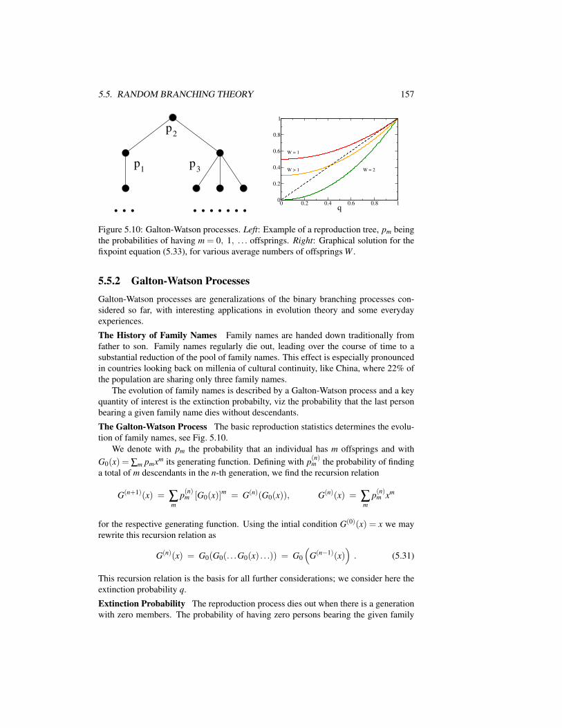
5.5. RANDOM BRANCHING THEORY 157
. . . . . . . . . .
p
p1
p3
2
0 0.2 0.4 0.6 0.8 1q
0
0.2
0.4
0.6
0.8
1
W = 1
W > 1 W = 2
Figure 5.10: Galton-Watson processes. Left: Example of a reproduction tree, pm beingthe probabilities of having m = 0, 1, . . . offsprings. Right: Graphical solution for thefixpoint equation (5.33), for various average numbers of offsprings W .
5.5.2 Galton-Watson ProcessesGalton-Watson processes are generalizations of the binary branching processes con-sidered so far, with interesting applications in evolution theory and some everydayexperiences.
The History of Family Names Family names are handed down traditionally fromfather to son. Family names regularly die out, leading over the course of time to asubstantial reduction of the pool of family names. This effect is especially pronouncedin countries looking back on millenia of cultural continuity, like China, where 22% ofthe population are sharing only three family names.
The evolution of family names is described by a Galton-Watson process and a keyquantity of interest is the extinction probabilty, viz the probability that the last personbearing a given family name dies without descendants.
The Galton-Watson Process The basic reproduction statistics determines the evolu-tion of family names, see Fig. 5.10.
We denote with pm the probability that an individual has m offsprings and withG0(x) = ∑m pmxm its generating function. Defining with p(n)m the probability of findinga total of m descendants in the n-th generation, we find the recursion relation
G(n+1)(x) = ∑m
p(n)m [G0(x)]m = G(n)(G0(x)), G(n)(x) = ∑
mp(n)m xm
for the respective generating function. Using the intial condition G(0)(x) = x we mayrewrite this recursion relation as
G(n)(x) = G0(G0(. . .G0(x) . . .)) = G0
(G(n−1)(x)
). (5.31)
This recursion relation is the basis for all further considerations; we consider here theextinction probability q.
Extinction Probability The reproduction process dies out when there is a generationwith zero members. The probability of having zero persons bearing the given family

158CHAPTER 5. CELLULAR AUTOMATA AND SELF-ORGANIZED CRITICALITY
name in the n-th generation is
q = p(n)0 = G(n)(0) = G0
(G(n−1)(0)
)= G0(q) , (5.32)
where we have used the recursion relation Eq. (5.31) and the stationary conditionG(n)(0) ≈ G(n−1)(0). The extinction probability q is hence given by the fixpoint q =G0(q) of the generating functional G0(x) of the reproduction probability.Binary Branching as a Galton-Watson Process As an example we consider the casethat
G0(x) = 1−W2+
W2
x2, G ′0(1) = W ,
viz that people may not have but either zero or two sons, with probabilities 1−W/2 andW/2< 1 respectively. The expected number of offsprings W is also called the fitness inevolution theory, see Chap. 6. This setting corresponds to the case of binary branching,see Fig. 5.8, with W/2 being the branching probability, describing the reproductivedynamics of unicellular bacteria.
The self-consistency condition (5.32) for the extinction probability q = q(W ) thenreads
q = 1−W2+
W2
q2, q(W ) =1
W±√
1W 2 −
(2−W )2
W 2 , (5.33)
with the smaller root being here of relevance. The extinction probability vanishes for areproduction rate of two,
q(W ) =
0 W = 2q ∈ ]0,1[ 1<W < 2
1 W ≤ 1
and is unity for a fitness below one, compare Fig. 5.10.
5.6 Application to Long-Term EvolutionAn application of the techniques developed in this chapter can be used to study a modelfor the evolution of species proposed by Bak and Sneppen.Fitness Landscapes Evolution deals with the adaption of species and their fitnessrelative to the ecosystem they live in.
Fitness Landscapes. The function that determines the chances of sur-vival of a species, its fitness, is called the fitness landscape.
In Fig. 5.11 a simple fitness landscape, in which there is only one dimension in thegenotype (or phenotype)2 space, is illustrated.
2The term “genotype” denotes the ensemble of genes. The actual form of an organism, the“phenotype”, is determined by the genotype plus environmental factors, like food supply duringgrowth.
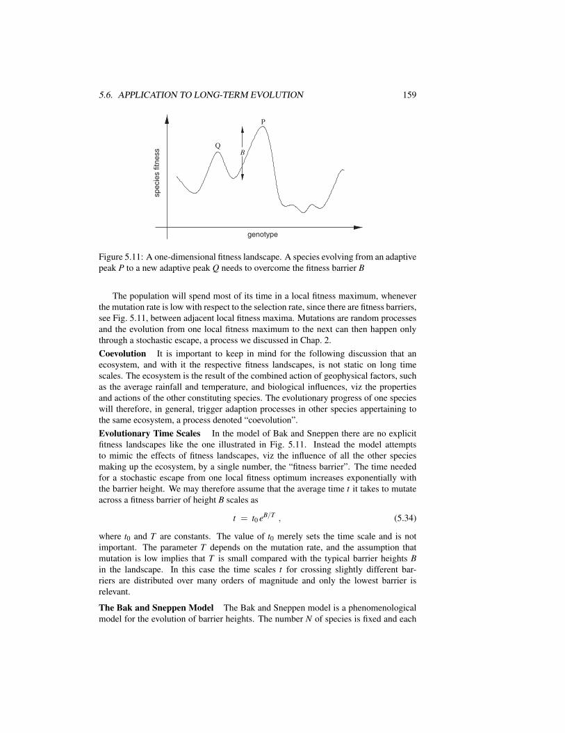
5.6. APPLICATION TO LONG-TERM EVOLUTION 159
genotype
specie
s fitness
B
P
Q
Figure 5.11: A one-dimensional fitness landscape. A species evolving from an adaptivepeak P to a new adaptive peak Q needs to overcome the fitness barrier B
The population will spend most of its time in a local fitness maximum, wheneverthe mutation rate is low with respect to the selection rate, since there are fitness barriers,see Fig. 5.11, between adjacent local fitness maxima. Mutations are random processesand the evolution from one local fitness maximum to the next can then happen onlythrough a stochastic escape, a process we discussed in Chap. 2.Coevolution It is important to keep in mind for the following discussion that anecosystem, and with it the respective fitness landscapes, is not static on long timescales. The ecosystem is the result of the combined action of geophysical factors, suchas the average rainfall and temperature, and biological influences, viz the propertiesand actions of the other constituting species. The evolutionary progress of one specieswill therefore, in general, trigger adaption processes in other species appertaining tothe same ecosystem, a process denoted “coevolution”.Evolutionary Time Scales In the model of Bak and Sneppen there are no explicitfitness landscapes like the one illustrated in Fig. 5.11. Instead the model attemptsto mimic the effects of fitness landscapes, viz the influence of all the other speciesmaking up the ecosystem, by a single number, the “fitness barrier”. The time neededfor a stochastic escape from one local fitness optimum increases exponentially withthe barrier height. We may therefore assume that the average time t it takes to mutateacross a fitness barrier of height B scales as
t = t0 eB/T , (5.34)
where t0 and T are constants. The value of t0 merely sets the time scale and is notimportant. The parameter T depends on the mutation rate, and the assumption thatmutation is low implies that T is small compared with the typical barrier heights Bin the landscape. In this case the time scales t for crossing slightly different bar-riers are distributed over many orders of magnitude and only the lowest barrier isrelevant.
The Bak and Sneppen Model The Bak and Sneppen model is a phenomenologicalmodel for the evolution of barrier heights. The number N of species is fixed and each

160CHAPTER 5. CELLULAR AUTOMATA AND SELF-ORGANIZED CRITICALITY
species has a respective barrier
Bi = Bi(t) ∈ [0,1], t = 0,1,2, . . .
for its further evolution. The initial Bi(0) are drawn randomly from [0,1]. The modelthen consists of the repetition of two steps:
(1) The times for a stochastic escape are exponentially distributed, see Eq. (5.34).It is therefore reasonable to assume that the species with the lowest barrier Bimutates and escapes first. After escaping, it will adapt quickly to a new localfitness maximum. At this point it will then have a new barrier for mutation,which is assumed to be uniformly distributed in [0,1].
(2) The fitness function for a species i is given by the ecological environment itlives in, which is made up of all the other species. When any given speciesmutates it therefore influences the fitness landscape for a certain number ofother species. Within the Bak and Sneppen model this translates into assigningnew random barriers B j for K−1 neighbors of the mutating species i.
The Bak and Sneppen model therefore tries to capture two essential ingredients oflong-term evolution: The exponential distribution of successful mutations and the in-teraction of species via the change of the overall ecosystem, when one constitutingspecies evolves.
The Random Neighbor Model The topology of the interaction between speciesin the Bak–Sneppen model is unclear. It might be chosen as two-dimensional, if thespecies are thought to live geographically separated, or one-dimensional in a toy model.In reality the topology is complex and can be assumed to be, in first approximation,random, resulting in the soluble random neighbor model.
Evolution of Barrier Distribution Let us discuss qualitatively the redistribution ofbarrier heights under the dynamics, the sequential repetition of step (1) and (2) above,see Fig. 5.12. The initial barrier heights are uniformly distributed over the interval[0,1] and the lowest barrier, removed in step (1), is small. The new heights reassignedin steps (1) and (2) will therefore lead, on the average, to an increase of the averagebarrier height with passing time.
With increasing average barrier height the characteristic lowest barrier is also raisedand eventually a steady state will be reached, just as in the sandpile model discussedpreviously. It turns out that the characteristic value for the lowest barrier is about 1/Kat equilibrium in the mean-field approximation and that the steady state is critical.Molecular Field Theory In order to solve the Bak–Sneppen model, we define thebarrier distribution function,
p(x, t) ,
viz the probability to find a barrier of hight x∈ [0,1] at time step t = 1,2, . . .. In addition,we define with Q(x) the probability to find a barrier above x:
Q(x) =∫ 1
xdx′ p(x′), Q(0) = 1, Q(1) = 0 . (5.35)

5.6. APPLICATION TO LONG-TERM EVOLUTION 161
60 80 100
species i
0.2
0.4
0.6
0.8
1
bar
rier
bi
species i
0
0.2
0.4
0.6
0.8
1
species i
0
0.2
0.4
0.6
0.8
1
40200
bar
rier
bi
bar
rier
bi
60 80 10040200 60 80 10040200
Figure 5.12: The barrier values (dots) for a 100 species one-dimensional Bak–Sneppen model after 50, 200 and 1600 steps of a simulation. The horizon-tal line in each frame represents the approximate position of the upper edge ofthe “gap”. A few species have barriers below this level, indicating that theywere involved in an avalanche at the moment when the snapshot of the systemwas taken
The dynamics is governed by the size of the smallest barrier. The distribution functionp1(x) for the lowest barrier is
p1(x) = N p(x)QN−1(x) , (5.36)
given by the probability p(x) for one barrier (out of the N barriers) to have the barrierheight x, while all the other N−1 barriers are larger. p1(x) is normalized,∫ 1
0dx p1(x) = (−N)
∫ 1
0dxQN−1(x)
∂Q(x)∂x
= −QN(x)∣∣∣x=1
x=0= 1 ,
where we used p(x) =−Q′(x), Q(0) = 1 and Q(1) = 0, see Eq. (5.35).Time Evolution of Barrier Distribution The time evolution for the barrier distribu-tion consists in taking away one (out of N) barrier, the lowest, via
p(x, t) − 1N
p1(x, t) ,
and by removing randomly K−1 barriers from the remaining N−1 barriers, and addingK random barriers:
p(x, t +1) = p(x, t) − 1N
p1(x, t) (5.37)
− K−1N−1
(p(x, t) − 1
Np1(x, t)
)+
KN.
We note that p(x, t + 1) is normalized whenever p(x, t) and p1(x, t) were normalizedcorrectly:∫ 1
0dx p(x, t +1) = 1− 1
N− K−1
N−1
(1− 1
N
)+
KN
=
(1− K−1
N−1
)N−1
N+
KN
=N−K
N+
KN≡ 1 .

162CHAPTER 5. CELLULAR AUTOMATA AND SELF-ORGANIZED CRITICALITY
Stationary Distribution After many iterations of Eq. (5.37) the barrier distributionwill approach a stationary solution p(x, t+1) = p(x, t)≡ p(x), as can be observed fromthe numerical simulation shown in Fig. 5.12. The stationary distribution correspondsto the fixpoint condition
0 = p1(x)1N
(K−1N−1
−1)− p(x)
K−1N−1
+KN
of Eq. (5.37). Using the expression p1 = N pQN−1, see Eq. (5.36), for p1(x) we thenhave
0 = N p(x)QN−1(x)(K−N) − p(x)(K−1)N + K(N−1) .
Using p(x) =− ∂Q(x)∂x we obtain
0 = N(N−K)∂Q(x)
∂xQN−1 + (K−1)N
∂Q(x)∂x
+ K(N−1)
0 = N(N−K)QN−1 dQ + (K−1)N dQ + K(N−1)dx .
We can integrate this last expression with respect to x,
0 = (N−K)QN(x) + (K−1)N Q(x) + K(N−1)(x−1) , (5.38)
where we took care of the boundary condition Q(1) = 0, Q(0) = 1.Solution in the Thermodynamic Limit The polynomial Eq. (5.38) simplifies in thethermodynamic limit, with N→ ∞ and K/N→ 0, to
0 = QN(x) + (K−1)Q(x) − K (1− x) . (5.39)
We note that Q(x) ∈ [0,1] and that Q(0) = 1, Q(1) = 0. There must therefore be somex ∈]0,1[ for which 0< Q(x)< 1. Then
QN(x)→ 0, Q(x) ≈ KK−1
(1− x) . (5.40)
Equation (5.40) remains valid as long as Q< 1, or x> xc:
1 =K
K−1(1− xc), xc =
1K.
We then have in the limit N→ ∞
limN→∞
Q(x) =
1 for x< 1/K
(1− x)K/(K−1) for x> 1/K , (5.41)
compare Fig. 5.13, and, using p(x) =−∂Q(x)/∂x,
limN→∞
p(x) =
0 for x< 1/K
K/(K−1) for x> 1/K . (5.42)

5.6. APPLICATION TO LONG-TERM EVOLUTION 163
0
at equilibrium
random
Q(x)
x1/K
0
1
1
Figure 5.13: The distribution Q(x) to find a fitness barrier larger than x ∈ [0,1] for theBak and Sneppen model, for the case of random barrier distribution (dashed line) andthe stationary distribution (dashed-dotted line), compare Eq. (5.41)
This result compares qualitatively well with the numerical results presented in Fig. 5.12.Note, however, that the mean-field solution Eq. (5.42) does not predict the exact criticalbarrier height, which is somewhat larger for K = 2 and a one-dimensional arrangementof neighbors, as in Fig. 5.12.1/N Corrections Equation (5.42) cannot be rigorously true for N <∞, since there is afinite probability for barriers with Bi < 1/K to reappear at every step. One can expandthe solution of the self-consistency Eq. (5.38) in powers of 1/N. One finds
p(x) '
K/N for x< 1/KK/(K−1) for x> 1/K . (5.43)
We leave the derivation as an exercise for the reader.Distribution of the Lowest Barrier If the barrier distribution is zero below the self-organized threshold xc = 1/K and constant above, then the lowest barrier must be belowxc with equal probability:
p1(x) →
K for x< 1/K0 for x> 1/K ,
∫ 1
0dx p1(x) = 1 . (5.44)
Equations (5.44) and (5.36) are consistent with Eq. (5.43) for x< 1/K.Coevolution and Avalanches When the species with the lowest barrier mutates weassign new random barrier heights to it and to its K − 1 neighbors. This causes anavalanche of evolutionary adaptations whenever one of the new barriers becomes thenew lowest fitness barrier. One calls this phenomenon “coevolution” since the evolu-tion of one species drives the adaption of other species belonging to the same ecosys-tem. We will discuss this and other aspects of evolution in more detail in Chap. 6.In Fig. 5.14 this process is illustrated for the one-dimensional model. The avalanchesin the system are clearly visible and well separated in time. In between the individ-ual avalanches the barrier distribution does not change appreciably; one speaks of a“punctuated equilibrium”.

164CHAPTER 5. CELLULAR AUTOMATA AND SELF-ORGANIZED CRITICALITY
0 20 40 60 80 100
species i
0
0.2
0.4
0.6
0.8
1
tim
e (a
rbit
rary
un
its)
Figure 5.14: A time series of evolutionary activity in a simulation of the one-dimensional Bak–Sneppen model with K = 2 showing coevolutionary avalanches in-terrupting the punctuated equilibrium. Each dot represents the action of choosing anew barrier value for one species
Critical Coevolutionary Avalanches In Sect. 5.5 we discussed the connection be-tween avalanches and random branching. The branching process is critical when itgoes on with a probability of 1/2. To see whether the coevolutionary avalanches withinthe Bak and Sneppen model are critical we calculate the probability pbran that at leastone of the K new, randomly selected, fitness barriers will be the new lowest barrier.
With probability x one of the new random barriers is in [0,x] and below the actuallowest barrier, which is distributed with p1(x), see Eq. (5.44). We then have
pbran = K∫ 1
0p1(x)xdx = K
∫ 1/K
0K xdx =
K2
2x2∣∣∣1/K
0≡ 1
2,
viz the avalanches are critical. The distribution of the size s of the coevolutionaryavalanches is then
D(s) ∼(
1s
)3/2
,
as evaluated within the random branching approximation, see Eq. (5.28), and indepen-dent of K. The size of a coevolutionary avalanche can be arbitrarily large and involve,in extremis, a finite fraction of the ecosystem, compare Fig. 5.14.
Features of the Critical State The sandpile model evolves into a critical state underthe influence of an external driving, when adding one grain of sand after another. Thecritical state is characterized by a distribution of slopes (or heights) zi, one of its char-acteristics being a discontinuity; there is a finite fraction of slopes with zi = Z−1, butno slope with zi = Z, apart from some of the sites participating in an avalanche.
In the Bak and Sneppen model the same process occurs, but without external driv-ings. At criticality the barrier distribution p(x) = ∂Q(x)/∂x has a discontinuity at

Exercises 165
xc = 1/K, see Fig. 5.13. One could say, cum grano salis, that the system has devel-oped an “internal phase transition”, namely a transition in the barrier distribution p(x),an internal variable. This emergent state for p(x) is a many-body or collective effect,since it results from the mutual reciprocal interactions of the species participating inthe formation of the ecosystem.
Exercises
SOLUTIONS OF THE LANDAU–GINZBURG FUNCTIONALDetermine the order parameter for h 6= 0 via Eq. (5.9) and Fig. 5.2. Discuss thelocal stability condition Eq. (5.3) for the three possible solutions and their globalstability. Note that F = f V , where F is the free energy, f the free energy densityand V the volume.
ENTROPY AND SPECIFIC HEAT WITHIN THE LANDAU MODELDetermine the entropy S(T ) = ∂F
∂T and the specific heat cV = T ∂S∂T within the
Landau–Ginzburg theory Eq. (5.1) for phase transitions.
THE GAME OF LIFEConsider the evolution of the following states, see Fig. 5.5, under the rules forConway’s game of life:
(0,0),(1,0),(0,1),(1,1)(0,-1),(0,0),(0,1)(0,0),(0,1),(1,0),(−1,0),(0,−1)(0,0),(0,1),(0,2),(1,2),(2,1)The predictions can be checked with Java-applets you may easily find in theInternet.
THE GAME OF LIFE ON A SMALL-WORLD NETWORKWrite a program to simulate the game of life on a 2D lattice. Consider thislattice as a network with every site having edges to its eight neighbors. Rewirethe network such that (a) the local connectivities zi ≡ 8 are retained for every siteand (b) a small-world network is obtained. This can be achieved by cutting twoarbitrary links with probability p and rewiring the four resulting stubs randomly.
Define an appropriate dynamical order parameter and characterize the changesas a function of the rewiring probability. Compare Chap. 1 and Chap. 2.
THE FOREST FIRE MODELDevelop a mean-field theory for the forest fire model by introducing appropriateprobabilities to find cells with trees, fires and ashes. Find the critical number ofnearest neighbors Z for fires to continue burning.
THE REALISTIC SANDPILE MODELPropose a cellular automata model that simulates the physics of real-world sand-piles somewhat more realistically than the BTW model. The cell values z(x,y)

166 5 Cellular Automata and Self-Organized Criticality
should correspond to the local height of the sand. Write a program to simulatethe model.
THE RANDOM BRANCHING MODELDerive the distribution of avalanche durations Eq. (5.29) in analogy to the stepsexplained in Sect. 5.5, by considering a recursion relation for the integrated du-ration probability Qn = ∑
nn′=0 Qn(0, p), viz for the probability that an avalanche
last maximally n time steps.
THE GALTON-WATSON PROCESSUse the fixpoint condition, Eq. (5.32) and show that the extinction probability isunity if the average reproduction rate is smaller than one.
THE BAK AND SNEPPEN MODELWrite a program to simulate the Bak and Sneppen model in Sect. 5.6 and com-pare it with the molecular field solution Eq. (5.38).
Further Reading
Introductory texts to cellular automata and to the game of life are Wolfram (1986),Creutz (1997) and Berlekamp et al. (1982). For a review of the forest fire and severalrelated models, see Clar et al. (1996); for a review of sandpiles, see Creutz (2004),and for a general review of self-organized criticality, see Paczuski and Bak (1999).Exemplary textbooks on statistical physics and phase transitions have been written byCallen (1985) and Goldenfeld (1992).
Some general features of 1/ f noise are discussed by Press (1978); its possiblerelation to self-organized criticality has been postulated by Bak et al. (1987). The for-mulation of the Bak and Sneppen (1993) model for long-term coevolutionary processesand its mean-field solution are discussed by Flyvbjerg et al. (1993).
The interested reader may also glance at some original research literature, such asa numerical study of the sandpile model (Priezzhev et al. 1996) and the application ofrandom branching theory to the sandpile model (Zapperi et al. 1995). The connectionof self-organized criticality to local conservation rules is worked out by Tsuchiya andKatori (2000), and the forest fire model with lightning is introduced by Drossel andSchwabl (1992).
BAK, P., SNEPPEN, K. 1993 Punctuated equilibrium and criticality in a simple model ofevolution. Physical Review Letters 71, 4083–4086.
BAK, P., TANG, C., WIESENFELD, K. 1987 Self-organized criticality: An explanation of1/ f noise. Physical Review Letters 59, 381–384.
BERLEKAMP, E., CONWAY, J., GUY, R. 1982 Winning Ways for Your Mathematical Plays,Vol. 2. Academic Press, New York.
CALLEN, H.B. 1985 Thermodynamics and Introduction to Thermostatistics. Wiley, NewYork.

Further Reading 167
CLAR, S., DROSSEL, B., SCHWABL, F. 1996 Forest fires and other examples of self-organizedcriticality. Journal of Physics: Condensed Matter 8, 6803–6824.
CREUTZ, M. 1997 Cellular automata and self-organized criticality. In G. Bhanot, S. Chenand P. Seiden (eds). Some New Directions in Science on Computers, pp. 147–169, WorldScientific, Singapore.
CREUTZ, M. 2004 Playing with sandpiles. Physica A 340, 521–526.
DROSSEL, B., SCHWABL, F. 1992 Self-organized critical forest-fire model. Physical ReviewLetters 69, 1629–1632.
FLYVBJERG, H., SNEPPEN, K., BAK, P. 1993 Mean field theory for a simple model of evo-lution. Physical Review Letters 71, 4087–4090.
GOLDENFELD, N. 1992 Lectures on Phase Transitions and the Renormalization Group. PerseusPublishing, Reading, MA.
NEWMAN, M.E.J., PALMER, R.G. 2002 Models of Extinction. Oxford University Press,New York.
PACZUSKI, M., BAK. P. 1999 Self organization of complex systems. In: Proceedings of 12thChris Engelbrecht Summer School; also available as http://www.arxiv.org/abs/cond-mat/9906077.
PRESS, W.H. 1978 Flicker noises in astronomy and elsewhere. Comments on Modern Physics,Part C 7, 103–119.
PRIEZZHEV, V.B., KTITAREV, D.V., IVASHKEVICH, E.V. 1996 Formation of avalanches andcritical exponents in an abelian sandpile model. Physical Review Letters 76, 2093–2096.
TSUCHIYA, T., KATORI, M. 2000 Proof of breaking of self-organized criticality in a noncon-servative abelian sandpile model. Physical Review Letters 61, 1183–1186.
WOLFRAM, S., EDITOR 1986 Theory and Applications of Cellular Automata. World Scien-tific, Singapore.
ZAPPERI, S., LAURITSEN, K.B., STANLEY, H.E. 1995 Self-organized branching processes:Mean-field theory for avalanches. Physical Review Letters 75, 4071–4074.

168 5 Cellular Automata and Self-Organized Criticality
Chapter 6
Darwinian Evolution,Hypercycles and Game Theory
Adaptation and evolution are quasi synonymous in popular language and Darwinianevolution is a prime application of complex adaptive system theory. We will see thatadaptation does not happen automatically and discuss the concept of “error catastro-phe” as a possible root for the downfall of a species. Venturing briefly into the mys-teries surrounding the origin of life, we will investigate the possible advent of a “qua-sispecies” in terms of mutually supporting hypercycles. The basic theory of evolutionis furthermore closely related to game theory, the mathematical theory of interactingagents, viz of rationally acting economic persons.
We will learn in this chapter, on the one hand, that every complex dynamical sys-tem has its distinct characteristics to be considered. In the case of Darwinian evolutionthese are concepts like fitness, selection and mutation. General notions from complexsystem theory are, on the other hand, important for a thorough understanding. An ex-ample is the phenomenon of stochastic escape discussed in Chap. 2, which is operativein the realm of Darwinian evolution.
6.1 Introduction
Microevolution The ecosystem of the earth is a complex and adaptive system. Itformed via Darwinian evolution through species differentiation and adaptation to achanging environment. A set of inheritable traits, the genome, is passed from parentto offspring and the reproduction success is determined by the outcome of randommutations and natural selection – a process denoted “microevolution”1
Asexual Reproduction. One speaks of asexual reproduction when anindividual has a single parent.
1Note that the term “macroevolution”, coined to describe the evolution at the level of organisms, isnowadays somewhat obsolete.
169

170CHAPTER 6. DARWINIAN EVOLUTION, HYPERCYCLES AND GAME THEORY
Here we consider mostly models for asexual reproduction, though most concepts canbe easily generalized to the case of sexual reproduction.
Basic Terminology Let us introduce some basic variables needed to formulate theapproach.
– Population M: The number of individuals.We assume here that M does not change with time, modeling the competition fora limited supply of resources.
– Genome N: Size of the genome.We encode the inheritable traits by a set of N binary variables,
s = (s1,s2, . . . ,sN), si = ±1 .
N is considered fixed.
– GenerationsWe consider time sequences of non-overlapping generations, like in a wheatfield. The population present at time t is replaced by their offspring at gener-ation t +1.
In Table 6.1 some typical values for the size N of the genome are listed. Note the threeorders of magnitude between simple eucaryotic life forms and the human genome.
State of the Population The state of the population at time t can be described byspecifying the genomes of all the individuals,
sα(t), α = 1 . . .M, s = (s1, . . . ,sN) .
We define byXs(t), ∑
sXs(t) = M , (6.1)
the number of individuals with genome s for each of the 2N points s in the genomespace. Typically, most of these occupation numbers vanish; biological populations areextremely sparse in genome space.
Combinatorial Genetics of Alleles Classical genetics focuses on the presence (orabsence) of a few characteristic traits. These traits are determined by specific sites,
Table 6.1: Genome size N and the spontaneous mutation rates µ , compare Eq. (6.3),per base for two RNA-based bacteria and DNA-based eucaryotes. From Jain and Krug(2006) and Drake et al. (1998)
Organism Genome size Rate per base Rate per genome
Bacteriophage Qβ 4.5 ×10³ 1.4 ×10⁻³ 6.5Bacteriophage λ 4.9 ×10⁴ 7.7 ×10⁻⁸ 0.0038E. Coli 4.6 ×10⁶ 5.4 ×10⁻¹⁰ 0.0025C. Elegans 8.0 ×10⁷ 2.3 ×10⁻¹⁰ 0.018Mouse 2.7 ×10⁹ 1.8 ×10⁻¹⁰ 0.49Human 3.2 ×10⁹ 5.0 ×10⁻¹¹ 0.16

6.2. MUTATIONS AND FITNESS IN A STATIC ENVIRONMENT 171
denoted “loci”, in the genome. The genetic realizations of these specific loci are called“alleles”. Popular examples are alleles for blue, brown and green eyes.
Combinatorial genetics deals with the frequency change of the appearance of agiven allele resulting from environmental changes during the evolutionary process.Most visible evolutionary changes are due to a remixing of alleles, as mutation in-duced changes in the genome are relatively rare; compare the mutation rates listed inTable 6.1.
Beanbag Genetics Without Epistatic Interactions One calls “epistasis” the fact thatthe effect of the presence of a given allele in a given locus may depend on which allelesare present in some other loci. Classical genetics neglects epistatic interactions. Theresulting picture is often called “beanbag genetics”, as if the genome were nothing buta bag carrying the different alleles within itself.
Genotype and Phenotype We note that the physical appearance of an organism is notdetermined exclusively by gene expression. One distinguishes between the genotypeand the phenotype.
– The Genotype: The genotype of an organism is the class to which that organismbelongs as determined by the DNA that was passed to the organism by its parentsat the organism’s conception.
– The Phenotype: The phenotype of an organism is the class to which that organ-ism belongs as determined by the physical and behavioral characteristics of theorganism, for example its size and shape, its metabolic activities and its patternof movement.
Selection acts, strictly speaking, only upon phenotypes, but only the genotype is be-queathed. The variations in phenotypes then act as a source of noise for the selectionprocess.
Speciation One denotes by “speciation” the process leading to the differentiationof an initial species into two distinct species. Speciation occurs due to adaptation todifferent ecological niches, often in distinct geographical environments. We will nottreat the various theories proposed for speciation here.
6.2 Mutations and Fitness in a Static Environment
Constant Environment We consider here the environment to be static; an assumptionthat is justified for the case of short-term evolution. This assumption clearly breaksdown for long time scales, as already discussed in Chap. 5 since the evolutionarychange of one species might lead to repercussions all over the ecosystem to whichit appertains.
Independent Individuals An important issue in the theory of evolution is the emer-gence of specific kinds of social behavior. Social behavior can only arise if the indi-viduals of the same population interact. We discuss some of these issues in Sect. 6.6 inthe context of game theory. Until then we assume non-interacting individuals, which

172CHAPTER 6. DARWINIAN EVOLUTION, HYPERCYCLES AND GAME THEORY
implies that the fitness of a given genetic trait is independent of the frequency of thisand of other alleles, apart from the overall competition for resources.Constant Mutation Rates We furthermore assume that the mutation rates are
– constant over time,
– independent of the locus in the genome, and
– not subject to genetic control.
Any other assumption would require a detailed microbiological modeling; a subjectbeyond our scope.Stochastic Evolution The evolutionary process can then be modeled as a three-stagestochastic process:
1. Reproduction: The individual α at generation t is the offspring of an individualα ′ living at generation t − 1. Reproduction is thus represented as a stochasticmap
α −→ α′ = Gt(α) , (6.2)
where Gt(α) is the parent of the individual α , and is chosen at random amongthe M individuals living at generation t−1.
2. Mutation: The genomes of the offspring differ from the respective genomes oftheir parents through random changes.
3. Selection: The number of surviving offspring of each individual depends on itsgenome; it is proportional to its “fitness”, which is a functional of the genome.
Point Mutations and Mutation Rate Here we consider mostly independent pointmutations, namely that every element of the genome is modified independently of theother elements,
sαi (t) = −sGt (α)
i (t−1) with probability µ , (6.3)
where the parameter µ ∈ [0,1/2] is the microscopic “mutation rate”. In real organisms,more complex phenomena take place, like global rearrangements of the genome, copiesof some part of the genome, displacements of blocks of elements from one location toanother, and so on. The values for the real-world mutation rates µ for various specieslisted in Table 6.1 are therefore to be considered as effective mutation rates.Fitness and Fitness Landscape The fitness W (s), also called “Wrightian fitness”,of a genotype trait s is proportional to the average number of offspring an individualpossessing the trait s has. It is strictly positive and can therefore be written as
W (s) = ekF(s)∝ average number of offspring of s. (6.4)
Selection acts in first place upon phenotypes, but we neglect here the difference, con-sidering the variations in phenotypes as a source of noise, as discussed above. Theparameters in Eq. (6.4) are denoted:

6.2. MUTATIONS AND FITNESS IN A STATIC ENVIRONMENT 173
Figure 6.1: (Smooth) one-dimensional model fitness landscapes F(s). Real-world fit-ness landscapes, however, contain discontinuities. Left: A fitness landscape with peaksand valleys, metaphorically also called a “rugged landscape”. Right: A fitness land-scape containing a single smooth peak, as described by Eq. (6.25)
– W (s): Wrightian fitness,
– F(s): fitness landscape,
– k: inverse selection temperature,2 and
– w(s): Malthusian fitness, when rewriting Eq. (6.4) as W (s) = ew(s)∆t ,where ∆t is the generation time.
We will work here with discrete time, viz with non-overlapping generations, and makeuse only of the Wrightian fitness W (s).Fitness of Individuals Versus Fitness of Species We remark that this notion of fitnessis a concept defined at the level of individuals in a homogeneous population. Theresulting fitness of a species or of a group of species needs to be explicitly evaluatedand is model-dependent.Fitness Ratios The assumption of a constant population size makes the reproductivesuccess a relative notion. Only the ratios
W (s1)
W (s2)=
ekF(s1)
ekF(s2)= ek[F(s1)−F((s2)] (6.5)
are important. It follows that the quantity W (s) is defined up to a proportionality con-stant and, accordingly, the fitness landscape F(s) only up to an additive constant, muchlike the energy in physics.The Fitness Landscape The graphical representation of the fitness function F(s) isnot really possible for real-world fitness functions, due to the high dimensional 2N ofthe genome space. It is nevertheless customary to draw a fitness landscape, like the oneshown in Fig. 6.1. However, one must bear in mind that these illustrations are not to betaken at face value, apart from model considerations.The Fundamental Theorem of Natural Selection The so-called fundamental the-orem of natural selection, first stated by Fisher in 1930, deals with adaptation in the
2The probability to find a state with energy E in a thermodynamic system with temperature T is pro-portional to the Boltzmann factor exp(−β E). The inverse temperature is β = 1/(kBT ), with kB being theBoltzmann constant.

174CHAPTER 6. DARWINIAN EVOLUTION, HYPERCYCLES AND GAME THEORY
absence of mutations and in the thermodynamic limit M→ ∞. An infinite populationsize allows one to neglect fluctuations.
The theorem states that the average fitness of the population cannot decrease intime under these circumstances, and that the average fitness becomes stationary onlywhen all individuals in the population have the maximal reproductive fitness.
The proof is straightforward. We define by
〈W 〉t ≡1M
M
∑α=1
W (sα(t)) =1M ∑
sW (s)Xs(t) , (6.6)
the average fitness of the population. Note that the ∑s in Eq. (6.6) contains 2N terms.The evolution equations are given in the absence of mutations by
Xs(t +1) =W (s)〈W 〉t
Xs(t) , (6.7)
where W (s)/〈W 〉t is the relative reproductive success. The overall population sizeremains constant,
∑s
Xs(t +1) =1〈W 〉t ∑
sXs(t)W (s) = M , (6.8)
where we have used Eq. (6.6) for 〈W 〉t . Then
〈W 〉t+1 =1M ∑
sW (s)Xs(t +1) =
1M ∑s W 2(s)Xs(t)1M ∑s′W (s′)Xs′(t)
=〈W 2〉t〈W 〉t
≥ 〈W 〉t , (6.9)
since 〈W 2〉t −〈W 〉2t = 〈∆W 2〉t ≥ 0. The steady state
〈W 〉t+1 = 〈W 〉t , 〈W 2〉t = 〈W 〉2t ,
is only possible when all individuals 1 . . .M in the population have the same fitness, vizthe same genotype.
6.3 Deterministic Evolution
Mutations are random events and the evolution process is therefore a stochastic process.But stochastic fluctuations become irrelevant in the limit of infinite population sizeM → ∞; they average out. In this limit the equations governing evolution becomedeterministic and only the average transition rates are relevant. One can then study indetail the condition necessary for adaptation to occur for various mutation rates.

6.3. DETERMINISTIC EVOLUTION 175
6.3.1 Evolution Equations
The Mutation Matrix The mutation matrix
Qµ(s′→ s), ∑s
Qµ(s′→ s) = 1 (6.10)
denotes the probabilities of obtaining a genotype s when attempting to reproduce anindividual with genotype s′. The mutation rates Qµ(s′→ s) may depend on a parameterµ determining the overall mutation rate. The mutation matrix includes the absence ofany mutation, viz the transition Qµ(s′→ s′). It is normalized.
Deterministic Evolution with Mutations We generalize Eq. (6.7), which is valid inthe absence of mutations, by including the effect of mutations via the mutation matrixQµ(s′→ s):
Xs(t +1)/M =
(∑s′
Xs′(t)W (s′)Qµ(s′→ s)
)/(∑s′
Ws′Xs′(t)
),
or
xs(t +1) =∑s′ xs′(t)W (s′)Qµ(s′→ s)
〈W 〉t, 〈W 〉t = ∑
s′Ws′xs′(t) , (6.11)
where we have introduced the normalized population variables
xs(t) =Xs(t)
M, ∑
sxs(t) = 1 . (6.12)
The evolution dynamics Eq. (6.11) retains the overall size ∑s Xs(t) of the population,due to the normalization of the mutation matrix Qµ(s′→ s), Eq. (6.10).
The Hamming Distance The Hamming distance
dH(s,s′) =N
∑i=1
(si− s′i)2
4=
N2− 1
2
N
∑i=1
sis′i (6.13)
measures the number of units that are different in two genome configurations s and s′,e.g. before and after the effect of a mutation event.
The Mutation Matrix for Point Mutations We consider the simplest mutation pat-tern, viz the case of fixed genome length N and random transcription errors afflictingonly individual loci. For this case, namely point mutations, the overall mutation prob-ability
Qµ(s′→ s) = µdH(1−µ)N−dH (6.14)
is the product of the independent mutation probabilities for all loci i = 1, . . . ,N, withdH denoting the Hamming distance dH(s,s′) given by Eq. (6.13) and µ the mutationrate µ defined in Eq. (6.3). One has
∑s
Qµ(s′→ s) = ∑dH
(NdH
)(1−µ)N−dN µ
dN = (1−µ +µ)N ≡ 1

176CHAPTER 6. DARWINIAN EVOLUTION, HYPERCYCLES AND GAME THEORY
and the mutation matrix defined by Eq. (6.14) is consequently normalized. We rewritethe mutation matrix as
Qµ(s′→ s) = ∝ exp([log(µ)− log(1−µ)]dH
)∝ exp
(β ∑
isis′i
), (6.15)
where we denoted by β an effective inverse temperature, defined by
β =12
log(
1−µ
µ
). (6.16)
The relation of the evolution equation (6.15) to the partition function of a thermo-dynamical system, hinted at by the terminology “inverse temperature” will becomeevident below.Evolution Equations for Point Mutations Using the exponential representationW (s) = exp[kF(s)], see Eq. (6.4), of the fitness W (s) and Eq. (6.15) for the mutationmatrix, we can write the evolution Eq. (6.12) via
xs(t +1) =1〈W 〉t ∑
s′xs′(t)exp
(β ∑
isis′i + kF(s′)
)(6.17)
in a form that is suggestive of a statistical mechanics analogy.Evolution Equations in Linear Form The evolution Eq. (6.17) is non-linear in thedynamical variables xs(t), due to the normalization factor 1/〈W 〉t . A suitable changeof variables does, however, allow the evolution equation to be cast into a linear form.
For this purpose we introduce the unnormalized variables ys(t) via
xs(t) =ys(t)
∑s′ ys′(t), 〈W 〉t = ∑
sW (s)xs(t) =
∑s W (s)ys(t)∑s′ ys′(t)
. (6.18)
Note that ys(t) are determined by Eq. (6.18) implicitly and that the normalization∑s′ ys′(t) can be chosen freely for every generation t = 1,2,3, . . .. The evolution Eq. (6.17)then becomes
ys(t +1) = Zt ∑s′
ys′(t)exp
(β ∑
isis′i + kF(s′)
), (6.19)
where
Zt =∑s′ ys′(t +1)∑s W (s)ys(t)
.
Choosing a different normalization for ys(t) and for ys(t +1) we may achieve Zt ≡ 1.Equation (6.19) is then linear in ys(t).Statistical Mechanics of the Ising Model In the following we will make use of analo-gies to notations commonly used in statistical mechanics. Readers who are unfamiliarwith the mathematics of the one-dimensional Ising model may skip the mathematicaldetails and concentrate on the interpretation of the results.

6.3. DETERMINISTIC EVOLUTION 177
We write the linear evolution Eq. (6.19) as
ys(t +1) = ∑s′
eβH[s,s′] ys′(t), ys(t+1) = ∑s(t)
eβH[s(t+1),s(t)] ys(t) , (6.20)
where we denote by H[s,s′] an effective Hamiltonian3
βH[s,s′] = β ∑i
sis′i + kF(s′) , (6.21)
and where we renamed the variables s by s(t + 1) and s′ by s(t). Equation (6.20) canbe solved iteratively,
ys(t+1) = ∑s(t),...,s(0)
eβH[s(t+1),s(t)] · · · eβH[s(1),s(0)] ys(0) , (6.22)
with the two-dimensional Ising-type Hamiltonian4
βH = β ∑i,t
si(t +1)si(t) + k∑t
F(s(t)) . (6.23)
A Short Detour: The Bra-ket Notation The evolution equation (6.22) can be carriedout in a straight-forward manner. For readers interested in the cross-correlations to thequantum mechanics of transfer matrices we make here a small detour into the Bra-ketnotation, which may otherwise be skipped.
One denotes with the “bra” 〈y| and with the “ket” |y〉 the respective row and columnvectors
〈y| = (y∗1,y∗2, . . . ,y
∗2N ), |y〉 =
y1...
y2N
, y j = ys
of a vector y, where y∗j is the conjugate complex of y j. Our variables are, however, allreal and y∗j ≡ y j. The scalar product x ·y of two vectors is then
x ·y ≡ ∑j
x∗j y j = 〈x|y〉 .
The expectation value 〈A〉y is given in bra-ket notation as
〈A〉y = ∑i, j
y∗i Ai j y j = 〈y|A|y〉 ,
where Ai j are the elements of the matrix A. In this notation we may rewrite the evolu-tion equation (6.22) as
ys(t+1) = 〈s(t +1)|eβH |y(0)〉 , (6.24)
with ys(t) = 〈s|y(t)〉. We are interested in the asymptotic limit t→∞ of the populationstate |y(t)>.
3The energy of a state depends in classical mechanics on the values of the available degrees of freedom,like the position and the velocity of a particle. This function is denoted Hamiltonian. In Eq. (6.21) theHamiltonian is a function of the binary variables s and s′.
4Any system of binary variables is equivalent to a system of interacting Ising spins, which retains onlythe classical contribution to the energy of interacting quantum mechanical spins (the magnetic moments).
178CHAPTER 6. DARWINIAN EVOLUTION, HYPERCYCLES AND GAME THEORY
6.3.2 Beanbag Genetics – Evolutions Without Epistasis
The Fujiyama Landscape The fitness function
F(s) =N
∑i=1
hisi, W (s) =N
∏i=1
ekhisi , (6.25)
is denoted the “Fujiyama landscape” since it corresponds to a single smooth peak asillustrated in Fig. 6.1. To see why, we consider the case hi > 0 and rewrite Eq. (6.25) as
F(s) = s0 · s, s0 = (h1,h2, . . . ,hN) .
The fitness of a given genome s is directly proportional to the scalar product with themaster sequence s0, with a well defined gradient pointing towards the master sequence.The Fujiyama Hamiltonian No epistatic interactions are present in the smooth peaklandscape Eq. (6.25). In terms of the corresponding Hamiltonian, seeEq. (6.23), this fact expresses itself as
βH = β
N
∑i=1
Hi, Hi = ∑t
si(t +1)si(t) +khi
β∑
tsi(t) . (6.26)
Every locus i corresponds exactly to the one-dimensional t = 1,2, . . . Ising-model βHiin an effective uniform magnetic field khi/β .The Transfer Matrix The Hamiltonian Eq. (6.26) does not contain interactions be-tween different loci of the genome; we can just consider a single Hamiltonian Hi andfind for the iterative solution Eq. (6.22)
〈yi(t +1)|eβHi |yi(0)〉 = 〈yi(t +1)|
(t
∏t ′=0
Tt ′
)|yi(0)〉 , (6.27)
with the 2×2 transfer matrix Tt = eβHi[si(t+1),si(t)] given by
(Tt)s,s′ = < s|Tt |s′ >, Tt =
(eβ+khi e−β
e−β eβ−khi
), (6.28)
where we have used s,s′ =±1 and the symmetrized form
βHi = β ∑t
si(t +1)si(t) +khi
2 ∑t
[si(t +1)+ si(t)
].
of the one-dimensional Ising model.Eigenvalues of the Transfer Matrix We consider
hi ≡ 1
and evaluate the eigenvalues ω of Tt :
ω2 − 2ω eβ cosh(k) + e2β − e−2β = 0 .

6.3. DETERMINISTIC EVOLUTION 179
The solutions are
ω1,2 = eβ cosh(k) ±√
e2β cosh2(k)− e2β + e−2β .
The larger eigenvalue ω1 thus has the form
ω1 = eβ cosh(k) +√
e2β sinh2(k)+ e−2β . (6.29)
Eigenvectors of the Transfer Matrix For ω1 > ω2 the eigenvector |ω1〉 correspond-ing to the larger eigenvalue ω1 dominates in the t→ ∞ limit and its components deter-mine the genome distribution. It is determined by(
〈+|ω1〉〈−|ω1〉
)=
(A+
A−
),
(eβ+k−ω1
)A+ + e−β A− = 0 ,
whereω1 − eβ+k =
√e2β sinh2(k)+ e−2β − eβ sinh(k) .
This yields(A+
A−
)=
1√Nω
(e−β√
e2β sinh2(k)+ e−2β − eβ sinh(k)
), (6.30)
with the normalization
Nω = A2++A2
− = e−2β + e2β sinh2(k)
+(
e2β sinh2(k)+ e−2β
)+2eβ sinh(k)
√e2β sinh2(k)+ e−2β
= 2e−2β + e2β sinh2(k)−2eβ sinh(k)√
e2β sinh2(k)+ e−2β .
The Order Parameter The one-dimensional Ising model does not have phase tran-sitions. Thus we reach the conclusion that evolution in the Fujiyama landscape takesplace in a single phase, where there is always some degree of adaptation. One canevaluate the amount of adaptation by introducing the order parameter5
m = limt→∞〈s(t)〉 = A+ − A− , (6.31)
which corresponds to the uniform magnetization in the Ising model analogy. One ob-tains
m =1
Nω
[e−β −
√e2β sinh2(k)+ e−2β + eβ sinh(k)
]. (6.32)
In order to interpret this result for the amount m of adaptation in the smooth Fujiyamalandscape we recall that (see Eqs. (6.16) and (6.4))
β =12
log(
1−µ
µ
), W (s) = ekF(s) ,
where µ is the mutation rate for point mutations. Thus we see that there is somedegree of adaptation whenever the fitness landscape does not vanish (k > 0). Note thatµ → 1/2, β → 0 corresponds to a diverging temperature in the Ising model analogy(6.26), but with an diverging effective magnetic field khi/β .
5The concept of order parameters in the theory of phase transition is discussed in Chap. 5.

180CHAPTER 6. DARWINIAN EVOLUTION, HYPERCYCLES AND GAME THEORY
6.3.3 Epistatic Interactions and the Error CatastropheThe result of the previous Sect. 6.3.2, i.e. the occurrence of adaptation in a smoothfitness landscape for any non-trivial model parameter, is due to the absence of epistaticinteractions in the smooth fitness landscape. Epistatic interactions introduce a phasetransition to a non-adapting regime once the mutation rate becomes too high.
The Sharp Peak Landscape One possibility to study this phenomenon is the limitingcase of very strong epistatic interactions; in this case, a single element of the genotypedoes not give any information on the value of the fitness. This fitness is defined by theequation
W (s) =1 if s = s0
1−σ otherwise. (6.33)
It is also denoted a fitness landscape with a “tower”. In this case, all genome sequenceshave the same fitness, which is lower than the one of the master sequence s0. The corre-sponding landscape F(s), defined by W (s) = ekF(s) is then equally discontinuous. Thislandscape has no gradient pointing towards the master sequence of maximal fitness.
Relative Notation We define by xk the fraction of the population whose genotype hasa Hamming distance k from the preferred genotype,
xk(t) =1M ∑
sδdH(s,s0),k Xs(t) . (6.34)
The evolution equations can be formulated entirely in terms of these xk; they corre-spond to the fraction of the population being k point mutations away from the mastersequence.
Infinite Genome Limit We take the N → ∞ limit and scale the mutation rate, seeEq. (6.3),
µ = u/N , (6.35)
for point mutations such that the average number of mutations
u = Nµ
occurring at every step remains finite.
The Absence of Back Mutations We consider starting from the optimal genome s0and consider the effect of mutations. Any successful mutation increases the distance kfrom the optimal genome s0. Assuming u 1 in Eq. (6.35) implies that
– multiple mutations do not appear, and that
– one can neglect back mutations that reduce the value of k, since they have arelative probability proportional to
kN− k
1 .
The Linear Chain Model The model so defined consequently has the structure of alinear chain. k = 0 being the starting point of the chain.

6.3. DETERMINISTIC EVOLUTION 181
x0 x1 x2 x3 x4
Figure 6.2: The linear chain model for the tower landscape, Eq. (6.33), with k denotingthe number of point mutations necessary to reach the optimal genome. The populationfraction xk+1(t +1) is only influenced by the value of xk and its own value at time t
We have two parameters: u, which measures the mutation rate and σ , which mea-sures the strength of the selection. Remembering that the fitness W (s) is proportionalto the number of offspring, see Eq. (6.33), we then find
x0(t +1) =1〈W 〉
[x0(t)(1−u)
], (6.36)
x1(t +1) =1〈W 〉
[ux0(t)+(1−u)(1−σ)x1(t)
]; (6.37)
xk(t +1) =1〈W 〉
[uxk−1(t)+(1−u)xk(t)
](1−σ) , k > 1, (6.38)
where 〈W 〉 is the average fitness. These equations describe a linear chain model asillustrated in Fig. 6.2. The population of individuals with the optimal genome x0 con-stantly loses members due to mutations. But it also has a higher number of offspringthan all other populations due to its larger fitness.Stationary Solution The average fitness of the population is given by
〈W 〉 = x0 + (1−σ)(1− x0) = 1−σ(1− x0) . (6.39)
We look for the stationary distribution x∗k. The equation for x∗0 does not involvethe x∗k with k > 0:
x∗0 =x∗0(1−u)
1−σ(1− x∗0), 1−σ(1− x∗0) = 1−u .
The solution is
x∗0 =
1−u/σ if u< σ
0 if u≥ σ, (6.40)
due to the normalization condition x∗0 ≤ 1. For u > σ the model becomes ill defined.The stationary solutions for the x∗k are for k = 1
x∗1 =u
1−σ(1− x∗0)− (1−u)(1−σ)x∗0 ,
which follows directly from Eqs. (6.37) and (6.39), and for k > 1
x∗k =(1−σ)u
1−σ(1− x∗0)− (1−u)(1−σ)x∗k−1 , (6.41)
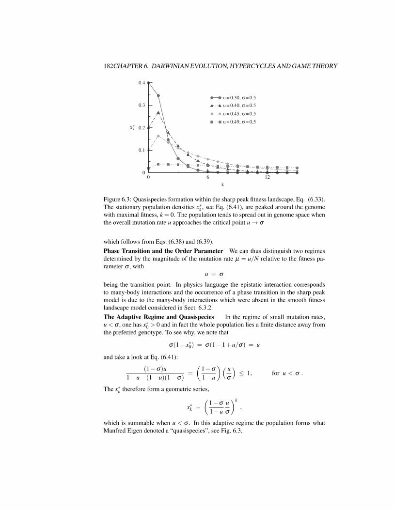
182CHAPTER 6. DARWINIAN EVOLUTION, HYPERCYCLES AND GAME THEORY
0 6 12
k
0
0.1
0.2
0.3
0.4
xk*
u = 0.30, σ = 0.5
u = 0.40, σ = 0.5
u = 0.45, σ = 0.5
u = 0.49, σ = 0.5
Figure 6.3: Quasispecies formation within the sharp peak fitness landscape, Eq. (6.33).The stationary population densities x∗k , see Eq. (6.41), are peaked around the genomewith maximal fitness, k = 0. The population tends to spread out in genome space whenthe overall mutation rate u approaches the critical point u→ σ
which follows from Eqs. (6.38) and (6.39).Phase Transition and the Order Parameter We can thus distinguish two regimesdetermined by the magnitude of the mutation rate µ = u/N relative to the fitness pa-rameter σ , with
u = σ
being the transition point. In physics language the epistatic interaction correspondsto many-body interactions and the occurrence of a phase transition in the sharp peakmodel is due to the many-body interactions which were absent in the smooth fitnesslandscape model considered in Sect. 6.3.2.The Adaptive Regime and Quasispecies In the regime of small mutation rates,u< σ , one has x∗0 > 0 and in fact the whole population lies a finite distance away fromthe preferred genotype. To see why, we note that
σ(1− x∗0) = σ(1−1+u/σ) = u
and take a look at Eq. (6.41):
(1−σ)u1−u− (1−u)(1−σ)
=
(1−σ
1−u
)( uσ
)≤ 1, for u < σ .
The x∗k therefore form a geometric series,
x∗k ∼(
1−σ
1−uuσ
)k
,
which is summable when u < σ . In this adaptive regime the population forms whatManfred Eigen denoted a “quasispecies”, see Fig. 6.3.

6.4. FINITE POPULATIONS AND STOCHASTIC ESCAPE 183
Quasispecies. A quasispecies is a population of genetically close butnot identical individuals.
The Wandering Regime and The Error Threshold In the regime of a large mu-tation rate, u > σ , we have x∗k = 0, ∀k. In this case, a closer look at the finite genomesituation shows that the population is distributed in an essentially uniform way overthe whole genotype space. The infinite genome limit therefore becomes inconsistent,since the whole population lies an infinite number of mutations away from the preferredgenotype. In this wandering regime the effects of finite population size are prominent.
Error Catastrophe. The transition from the adaptive (quasispecies)regime to the wandering regime is denoted the “error threshold” or “errorcatastrophe”.
The notion of error catastrophe is a quite generic feature of quasispecies theory, inde-pendent of the exact nature of the fitness landscape containing epistatic interactions. Aquasispecies can no longer adapt, once its mutation rate becomes too large. In the realworld the error catastrophe implies extinction.
6.4 Finite Populations and Stochastic Escape
Punctuated Equilibrium Evolution is not a steady process, there are regimes of rapidincrease of the fitness and phases of relative stasis. This kind of overall dynamicalbehavior is denoted the “punctuated equilibrium”.
In this context, adaptation can result either from local optimization of the fitness ofa single species or via coevolutionary avalanches, as discussed in Chap. 5.
The Neutral Regime. The stage where evolution is essentially drivenby random mutations is called the neutral (or wandering) regime.
The quasispecies model is inconsistent in the neutral regime. In fact, the populationspreads out in genome space in the neutral regime and the infinite population limit isno longer reachable. In this situation, the fluctuations of the reproductive process in afinite population have to be taken into account.
Deterministic Versus Stochastic Evolution Evolution is driven by stochastic pro-cesses, since mutations are random events. Nevertheless, randomness averages out andthe evolution process becomes deterministic in the thermodynamic limit, as discussedin Sect. 6.3, when the number M of individuals diverges, M→ ∞.
Evolutionary processes in populations with a finite number of individuals differfrom deterministic evolution quantitatively and sometimes also qualitatively, the laterbeing our focus of interest here.
Stochastic Escape. Random mutations in a finite population mightlead to a decrease in the fitness and to a loss of the local maximum in thefitness landscape with a resulting dispersion of the quasispecies.

184CHAPTER 6. DARWINIAN EVOLUTION, HYPERCYCLES AND GAME THEORY
We have given a general account of the theory of stochastic escape in Chap. 2. Here wewill discuss in some detail under which circumstances this phenomenon is importantin evolutionary processes of small populations.
6.4.1 Strong Selective Pressure and Adaptive Climbing
Adaptive Walks We consider a coarse-grained description of population dynamicsfor finite populations. We assume that
(a) the population is finite,
(b) the selective pressure is very strong, and
(c) the mutation rate is small.
It follows from (b) that one can represent the population by a single point in genomespace; the genomes of all individuals are taken to be equal. The evolutionary dynamicsis then the following:
(A) At each time step, only one genome element of some individual in the populationmutates.
(B) If, because of this mutation, one obtains a genotype with higher fitness, the newgenotype spreads rapidly throughout the entire population, which then movesaltogether to the new position in genome space.
(C) If the fitness of the new genotype is lower, the mutation is rejected and the popu-lation remains at the old position.
Physicists would call this type of dynamics a Monte Carlo process at zero temper-ature. As is well known, this algorithm does not lead to a global optimum, but to a“typical” local optimum. Step (C) holds only for the infinite population limit. We willrelax this condition further below.
The Random Energy Model It is thus important to investigate the statistical prop-erties of the local optima, which depend on the properties of the fitness landscape. Asuitable approach is to assume a random distribution of the fitness.
The Random Energy Model. The fitness landscape F(s) is uniformlydistributed between 0 and 1.
The random energy model is illustrated in Fig. 6.4. It captures, as we will see fur-ther below two ingredients expected for real-world fitness landscapes, namely a largenumber of local fitness optima close to the global fitness maximum.
Local Optima in the Random Energy Model Let us denote by N the number ofgenome elements. The probability that a point with fitness F(s) is a local optimum issimply given by
FN = FN(s) ,

6.4. FINITE POPULATIONS AND STOCHASTIC ESCAPE 185
0
1
N = 2
Figure 6.4: Local fitness optima in a one-dimensional random fitness distribution; thenumber of neighbors is two. This simplified picture does not corresponds directly tothe N = 2 random energy model, for which there are just 22 = 4 states in genomespace. It shows, however, that random distributions may exhibit an enormous numberof local optima (filled circles), which are characterized by lower fitness values both onthe left-hand side as well as on the right-hand side
since we have to impose that the N nearest neighbors
(s1, . . . ,−si, . . . ,sN), (i = 1, . . . ,N), s = (s1, . . . ,sN) ,
of the point have fitness less than F . The probability that a point in genome space is alocal optimum is given by
Plocal optimum =∫ 1
0FNdF =
1N +1
, (6.42)
since the fitness F is equally distributed in [0,1]. There are therefore many local optima,namely 2N/(N + 1). A schematic picture of the large number of local optima in arandom distribution is given in Fig. 6.4.Average Fitness at a Local Optimum The typical fitness of a local optimum is
Ftyp =1
1/(N +1)
∫ 1
0F FNdF =
N +1N +2
=1+1/N1+2/N
≈ 1−1/N , (6.43)
viz very close the global optimum of 1, when the genome length N is large. At everysuccessful step the distance from the top is divided, on average, by a factor of 2.Successful Mutations We now consider the adaptation process. Any mutation resultsin a randomly distributed fitness of the offspring. A mutation is successful wheneverthe fitness of the offspring is bigger than the fitness of its parent. The typical fitnessattained after ` successful steps is then of the order of
1− 12`+1 ,
when starting (l = 0) from an average initial fitness of 1/2. It follows that the typicalnumber of successful mutations after which an optimum is attained is
Ftyp = 1−1/N = 1− 12`typ+1 , `typ +1 =
logNlog2
, (6.44)

186CHAPTER 6. DARWINIAN EVOLUTION, HYPERCYCLES AND GAME THEORY
different genotypes
pesc
Fit
nes
s F
climbing
Figure 6.5: Climbing process and stochastic escape. The higher the fitness, the moredifficult it becomes to climb further. With an escape probability pesc the populationjumps somewhere else and escapes a local optimum
i.e. it is relatively small.The Time Needed for One Successful Mutation Even though the number of suc-cessful mutations Eq. (6.44) needed to arrive at the local optimum is small, the time toclimb to the local peak can be very long; see Fig. 6.5 for an illustration of the climbingprocess.
We define by
tF = ∑n
nPn, n : number of generations
the average number of generations necessary for the population with fitness F to achieveone successful mutation, with Pn being the probability that it takes exactly n genera-tions. We obtain:
tF = 1(1−F) + 2(1−F)F + 3(1−F)F2 + 4(1−F)F3 + · · ·
=1−F
F
∞
∑n=0
nFn =1−F
F
(F
∂
∂F
∞
∑n=0
Fn
)= (1−F)
∂
∂F1
1−F
=1
1−F. (6.45)
The average number of generations necessary to further increase the fitness by a suc-cessful mutation diverges close to the global optimum F → 1.
The Total Climbing Time Every successful mutation decreases the distance 1−F tothe top by 1/2 and therefore increases the factor 1/(1−F) on the average by 2. Thetypical number `typ, see Eq. (6.44), of successful mutations needed to arrive at a localoptimum determines, via Eq. (6.45), the expected total number of generations Topt toarrive at the local optimum. It is therefore on the average
Topt = 1 tF + 2 tF + 22 tF + . . . + 2`typtF
= tF1−2`typ+1
1−2≈ tF 2`typ+1 = tF e(`typ+1) log2

6.4. FINITE POPULATIONS AND STOCHASTIC ESCAPE 187
≈ tF elogN =N
1−F≈ 2N , (6.46)
where we have used Eq. (6.44) and F ≈ 1/2 for a typical starting fitness. The timeneeded to climb to a local maximum in the random fitness landscape is therefore pro-portional to the length of the genome.
6.4.2 Adaptive Climbing Versus Stochastic EscapeIn Sect. 6.4.1 the average properties of adaptive climbing have been evaluated. We nowtake the fluctuations in the reproductive process into account and compare the typicaltime scales for a stochastic escape with those for adaptive climbing.
Escape Probability When a favorable mutation appears it spreads instantaneouslyinto the whole population, under the condition of strong selection limit, as assumed inour model.
We consider a population situated at a local optimum or very close to a local op-timum. Every point mutation then leads to a lower fitness and the probability pesc forstochastic escape is
pesc ≈ uM ,
where M is the number of individuals in the population and u ∈ [0,1] the mutation rateper genome, per individual and per generation, compare Eq. (6.35). The escape canonly happen when a mutation occurs in every member of the population within thesame generation (see also Fig. 6.5). If a single individual does not mutate it retains itshigher fitness of the present local optimum and all other mutations are discarded withinthe model, assuming a strong selective pressure.
Stochastic Escape and Stasis We now consider a population climbing towards a localoptimum. The probability that the fitness of a given individual increases is (1−F)u.It needs to mutate with a probability u and to achieve a higher fitness, when mutating,with probability 1−F . We denote by
a = 1− (1−F)u
the probability that the fitness of an individual does not increase with respect to thecurrent fitness F of the population. The probability qbet that at least one better genotypeis found is then given by
qbet = 1−aM .
Considering a population close to a local optimum, a situation typical for real-worldecosystems, we can then distinguish between two evolutionary regimes:
– Adaptive Walk: The escape probability pesc is much smaller than the probabilityto increase the fitness, qbet pesc. The population continuously increases itsfitness via small mutations.
– The Wandering Regime: Close to a local optimum the adaptive dynamics slowsdown and the probability of stochastic escape pesc becomes comparable to thatof an adaptive process, pesc ≈ qbet. The population wanders around in genomespace, starting a new adaptive walk after every successful escape.
188CHAPTER 6. DARWINIAN EVOLUTION, HYPERCYCLES AND GAME THEORY
Typical Escape Fitness During the adaptive walk regime the fitness F increasessteadily, until it reaches a certain typical fitness Fesc for which the probability of stochas-tic escape becomes substantial, i.e. when pesc ≈ qbet and
pesc = uM = 1− [1− (1−Fesc)u]M = qbet
holds. As (1−Fesc) is then small we can expand the above expression in (1−Fesc),
uM ≈ 1− [1−M(1−Fesc)u] = M(1−Fesc)u ,
obtaining1−Fesc = uM−1/M . (6.47)
The fitness Fesc necessary for the stochastic escape to become relevant is exponentiallyclose to the global optimum F = 1 for large populations M.
The Relevance of Stochastic Escape The stochastic escape occurs when a localoptimum is reached, or when we are close to a local optimum. We may estimate theimportance of the escape process relative to that of the adaptive walk by comparing thetypical fitness Ftyp of a local optimum achieved by a typical climbing process with thetypical fitness Fesc needed for the escape process to become important:
Ftyp = 1− 1N≡ Fesc = 1− uM−1
M,
1N
=uM−1
M,
where we have used Eq. (6.43) for Ftyp. The last expression is now independent of thedetails of the fitness landscape, containing only the measurable parameters N, M and u.This condition can be fulfilled only when the number of individuals M is much smallerthan the genome length N, as u< 1. The phenomenon of stochastic escape occurs onlyfor very small populations.
6.5 Prebiotic EvolutionPrebiotic evolution deals with the question of the origin of life. Is it possible to definechemical autocatalytic networks in the primordial soup having properties akin to thoseof the metabolistic reaction networks going on continuously in every living cell?
6.5.1 Quasispecies TheoryThe quasispecies theory was introduced by Manfred Eigen to describe the evolutionof a system of information carrying macromolecules through a set of equations forchemical kinetics,
ddt
xi = xi = Wiixi + ∑j 6=i
Wi jx j − xiφ(t) , (6.48)
where the xi denote the concentrations of i= 1 . . .N molecules. Wii is the (autocatalytic)self-replication rate and the off-diagonal terms Wi, j (i 6= j) the respective mutation rates.

6.5. PREBIOTIC EVOLUTION 189
Mass Conservation We can choose the flux −xφ(t) in Eigen’s equations (6.48) forprebiotic evolution such that the total concentration C, viz the total mass
C = ∑i
xi
is conserved for long times. Summing Eq. (6.48) over i we obtain
C = ∑i j
Wi jx j −C φ , φ(t) = ∑i j
Wi jx j(t) , (6.49)
for a suitable choice for the field φ(t), leading to
C = φ (1−C),ddt(C−1) = −φ (C−1) . (6.50)
The total concentration C(t) will therefore approach 1 for t → ∞ for φ > 0, whichwe assume to be the case here, implying total mass conservation. In this case theautocatalytic rates Wii dominate with respect to the transmolecular mutation rates Wi j(i 6= j).Quasispecies We can write the evolution equation (6.48) in matrix form
ddt
x(t) = (W −1φ) x(t), x =
x1x1· · ·xN
, (6.51)
where W is the matrix Wi j. We assume here for simplicity a symmetric mutationmatrix Wi j =Wji. The solutions of the linear differential equation (6.51) are then givenin terms of the eigenvectors~eλ of W :
Weλ = λ eλ , x(t) = ∑λ
aλ (t) eλ , aλ = [λ −φ(t)]aλ .
The eigenvector eλmax with the largest eigenvalue λmax will dominate for t→∞, due tothe overall mass conservation Eq. (6.50). The flux will adapt to the largest eigenvalue,
limt→∞
(λmax−φ(t)
)→ 0 ,
leading to the stationary condition xi = 0 for the evolution Eq. (6.51) in the long timelimit.
If W is diagonal (no mutations) a single macromolecule will remain in the primor-dial soup for t→ ∞. For small but finite mutation rates Wi j (i 6= j), a quasispecies willemerge, made up of different but closely related macromolecules.The Error Catastrophe The mass conservation equation (6.50) cannot be retainedwhen the mutation rates become too big, viz when the eigenvectors ~eλ become ex-tended. In this case the flux φ(t) diverges, see Eq. (6.49), and the quasispecies modelconsequently becomes inconsistent. This is the telltale sign of the error catastrophe.

190CHAPTER 6. DARWINIAN EVOLUTION, HYPERCYCLES AND GAME THEORY
A B
Figure 6.6: The simplest hypercycle. A and B are self-replicating molecules. A actsas a catalyst for B, i.e. the replication rate of B increases with the concentration of A.Likewise the presence of B favors the replication of A
The quasispecies model Eq. (6.48) is equivalent to the random energy model formicroevolution studied in Sect. 6.4, with the autocatalytic rates Wii corresponding tothe fitness of the xi, which corresponds to the states in genome space. The analysiscarried through in Sect. 6.3.3 for the occurrence of an error threshold is therefore alsovalid for Eigen’s prebiotic evolutionary equations.
6.5.2 Hypercycles and Autocatalytic Networks
RNA World The macromolecular evolution equations (6.48) do not contain termsdescribing the catalysis of molecule i by molecule j. This process is, however, impor-tant both for the prebiotic evolution, as stressed by Manfred Eigen, as well as for theprotein reaction network in living cells.
Hypercycles. Two or more molecules may form a stable catalytic(hyper) cycle when the respective intermolecular catalytic rates are largeenough to mutually support their respective synthesis.

6.5. PREBIOTIC EVOLUTION 191
I1I1
In
I4I3
I2In
I4I3
I2
par
kpar
(a) (b)
Figure 6.7: Hypercycles of higher order. (a) A hypercycle of order n consists of ncyclically coupled self-replicating molecules Ii, and each molecule provides catalyticsupport for the subsequent molecule in the cycle. (b) A hypercycle with a single self-replicating parasitic molecule “par” coupled to it via kpar. The parasite gets catalyticsupport from I2 but does not give back catalytic support to the molecules in the hyper-cycle
An illustration of some hypercycles is given in Figs. 6.6 and 6.7. The most likelychemical candidate for the constituent molecules is RNA, functioning both enzymati-cally and as a precursor of the genetic material. One speaks also of an “RNA world”.
Reaction Networks We disregard mutations in the following and consider the cat-alytic reaction equations
xi = xi
(λi +∑
jκi jx j−φ
)(6.52)
φ = ∑k
xk
(λk +∑
jκk jx j
), (6.53)
where xi are the respective concentrations, λi the autocatalytic growth rates and κi j thetransmolecular catalytic rates. The field φ has been chosen, Eq. (6.53), such that thetotal concentration C = ∑i xi remains constant
C = ∑i
xi = ∑i
xi
(λi +∑
jκi jx j
)−C φ = (1−C)φ → 0
for C→ 1.
The Homogeneous Network We consider the case of homogeneous “interactions”κi6= j and uniformly distributed autocatalytic growth rates:
κi 6= j = κ, κii = 0, λi = α i , (6.54)
compare Fig. 6.8, leading to
xi = xi
(λi +κ ∑
j 6=ix j−φ
)= xi
(λi +κ−κxi−φ
), (6.55)

192CHAPTER 6. DARWINIAN EVOLUTION, HYPERCYCLES AND GAME THEORY
0
0.05
0.1
0.15
0.2
0.25
xi*
xi* : ω = 50
xi* : ω = 200
xi* : ω = 450
0 50
i
0
20
40
λi
403010 20
Figure 6.8: The autocatalytic growth rates λi (left axis), as in Eq. (6.54) with α = 1,and the stationary solution x∗i (right axis) of the concentrations, Eq. (6.57), constitutinga prebiotic quasispecies, for various mean intercatalytic rates κ ≡ ω . The horizontalaxis i = 1,2, . . . ,50 denotes the respective molecules
where we have used ∑i xi = 1. The fixed points x∗i of Eq. (6.55) are
x∗i =
(λi +κ−φ)/κ
0 λi = α,2α, . . . ,Nα , (6.56)
where the non-zero solution is valid for λi−κ−φ > 0. The flux φ in Eq. (6.56) needsto obey Eq. (6.53), as the self-consistency condition.The Stationary Solution The case of homogeneous interactions, Eq. (6.54), can besolved analytically. Dynamically, the xi(t) with the largest growth rates λi will dom-inate and obtain a non-zero steady-state concentration x∗i . We may therefore assumethat there exists an N∗ ∈ [1,N] such that
x∗i =
(λi +κ−φ)/κ N∗ ≤ i≤ N
0 1≤ i< N∗ , (6.57)
compare Fig. 6.8, where N∗ and φ are determined by the normalization condition
1 =N
∑i=N∗
x∗i =N
∑i=N∗
λi +κ−φ
κ=
α
κ
N
∑i=N∗
i+[
κ−φ
κ
](N +1−N∗
)=
α
2κ
[N(N +1)−N∗(N∗−1)
]+
[κ−φ
κ
](N +1−N∗
)(6.58)
and by the condition that x∗i = 0 for i = N∗−1:
0 =λN∗−1 +κ−φ
κ=
α(N∗−1)κ
+κ−φ
κ. (6.59)

6.6. COEVOLUTION AND GAME THEORY 193
We eliminate (κ−φ)/κ from Eqs. (6.58) and (6.59) for large N, N∗:
2κ
α' N2− (N∗)2−2N∗ (N−N∗)
= N2−2N∗N +(N∗)2 = (N−N∗)2 .
The number of surviving species N−N∗ is therefore
N−N∗ '√
2κ
α, (6.60)
which is non-zero for a finite and positive inter-molecular catalytic rate κ . A hypercycleof mutually supporting species (or molecules) has formed.The Origin of Life The scientific discussions concerning the origin of life are highlycontroversial to date and it is speculative whether hypercycles have anything to do withit. Hypercycles describe closed systems of chemical reactions which have to come toa stillstand eventually, as a consequence of the continuous energy dissipation. In fact,a tellpoint sign of biological activities is the buildup of local structures, resulting in alocal reduction of entropy, possible only at the expense of an overall increase of theenvironmental entropy. Life, as we understand it today, is possible only as an opensystem driven by a constant flux of energy.
Nevertheless it is interesting to point out that Eq. (6.60) implies a clear divisionbetween molecules i = N∗, . . . , N which can be considered to form a primordial “lifeform” separated by molecules i = 1, . . . ,N∗−1 belonging to the “environment”, sincethe concentrations of the latter are reduced to zero. This clear separation betweenparticipating and non-participating substances is a result of the non-linearity of thereaction equations (6.52). The linear evolution equations (6.48) would, on the otherhand, result in a continuous density distribution, as illustrated in Fig. 6.3 for the caseof the sharp peak fitness landscape. One could then conclude that life is possible onlyvia cooperation, resulting from non-linear evolution equations.
6.6 Coevolution and Game TheoryThe average number of offsprings, viz the fitness, is the single relevant reward functionwithin Darwinian evolution. There is hence a direct connection between evolutionaryprocesses and game theory, which deals with interacting agents trying to maximize asingle reward function denoted utility. Several types of games may be considered inthis context, namely games of interacting species giving rise to coevolutionary phenom-ena or games of interacting members of the same species, pursuing distinct behavioralstrategies.Coevolution In the discussion so far we first considered the evolution of a singlespecies and then in Sect. 6.5.2, the stabilization of an “ecosystem” made of a hypercycleof mutually supporting species.
Coevolution. When two or more species form an interdependentecosystem the evolutionary progress of part of the ecosystem will gen-erally induce coevolutionary changes also in the other species.

194CHAPTER 6. DARWINIAN EVOLUTION, HYPERCYCLES AND GAME THEORY
sequence space S sequence space S
x(S)
F(S)
sequence space S sequence space S
x(S)
F(S)
Figure 6.9: Top: Evolutionary process of a single (quasi) species in a fixed fitnesslandscape (fixed ecosystem), here with tower-like structures, see Eq. (6.33). Bottom: Acoevolutionary process might be regarded as changing the respective fitness landscapes
One can view the coevolutionary process also as a change in the respective fitnesslandscapes, see Fig. 6.9. A prominent example of phenomena arising from coevolutionis the “red queen” phenomenon.
The Red Queen Phenomenon. When two or more species are inter-dependent then “It takes all the running, to stay in place” (from LewisCarroll’s children’s book “Through the Looking Glass”).
A well-known example of the red queen phenomenon is the “arms race” between preda-tor and prey commonly observed in natural ecosystems.The Green World Hypothesis Plants abound in real-world ecosystems, geologyand climate permitting, they are rich and green. Naively one may expect that her-bivores should proliferate when food is plenty, keeping vegetation constantly down.This doesn’t seem to happen in the world and Hairston, Smith and Slobodkin proposedthat coevolution gives rise to a trophic cascade, where predators keep the herbivoressubstantially below the support level of the bioproductivity of the plants. This “greenworld hypothesis” arises natural in evolutionary models, but has been difficult to verifyin field studies.Avalanches and Punctuated Equilibrium In Chap. 5 we discussed the Bak andSneppen model of coevolution. It may explain the occurrence of coevolutionary avalancheswithin a state of punctuated equilibrium.
Punctuated Equilibrium. Most of the time the ecosystem is in equi-librium, in the neutral phase. Due to rare stochastic processes periods ofrapid coevolutionary processes are induced.
The term punctuated equilibrium was proposed by Gould and Eldredge in 1972 to de-scribe a characteristic feature of the evolution of simple traits observed in fossil records.

6.6. COEVOLUTION AND GAME THEORY 195
In contrast to the gradualistic view of evolutionary changes, these traits typically showlong periods of stasis interrupted by very rapid changes.
The random events leading to an increase in genome optimization might be a raremutation bringing one or more individuals to a different peak in the fitness landscape(microevolution) or a coevolutionary avalanche.Strategies and Game Theory One is often interested, in contrast to the stochasticconsiderations discussed so far, in the evolutionary processes giving rise to very spe-cific survival strategies. These questions can be addressed within game theory, whichdeals with strategically interacting agents in economics and beyond. When an ani-mal meets another animal it has to decide, to give an example, whether confrontation,cooperation or defection is the best strategy. The basic elements of game theory are:
– Utility: Every participant, also called an agent, plays for himself, trying to max-imize its own utility.
– Strategy: Every participant follows a set of rules of what to do when encounter-ing an opponent; the strategy.
– Adaptive Games: In adaptive games the participants change their strategy inorder to maximize future return. This change can be either deterministic orstochastic.
– Zero-Sum Games: When the sum of utilities is constant, you can only win whatthe others lose.
– Nash Equilibrium: Any strategy change by a participant leads to a reduction ofhis utility.
Hawks and Doves This simple evolutionary game tries to model competition in termsof expected utilities between aggressive behavior (by the “hawk”) and peaceful (by the“dove”) demeanor. The rules are:Dove meets Dove ADD =V/2 They divide the territory.Hawk meets Dove AHD =V , ADH = 0 The Hawk gets all the territory, the
Dove retreats and gets nothing.Hawk meets Hawk AHH = (V −C)/2 They fight, get injured, and win
half the territory.
The expected returns, the utilities, can be cast in matrix form,
A =
(AHH AHDADH ADD
)=
( 12 (V −C) V
0 V2
).
A is denoted the “payoff” matrix. The question is then, under which conditions it paysto be peaceful or aggressive.

196CHAPTER 6. DARWINIAN EVOLUTION, HYPERCYCLES AND GAME THEORY
Adaptation by Evolution The introduction of reproductive capabilities for the par-ticipants turns the hawks-and-doves game into an evolutionary game. In this contextone considers the behavioral strategies to result from the expression of distinct alleles.
The average number of offspring of a player is proportional to its fitness, which inturn is assumed to be given by its expected utility,
xH =(
AHHxH +AHDxD−φ(t))
xH
xD =(
ADHxH +ADDxD−φ(t))
xD, (6.61)
where xD and xH are the density of doves and hawks, respectively, and where the flux
φ(t) = xHAHHxH + xHAHDxD + xDADHxH + xDADDxD
ensures an overall constant population, xH + xD = 1.The Steady State Solution We are interested in the steady-state solution ofEq. (6.61), with xD = 0 = xH . Setting
xH = x, xD = 1− x ,
we find
φ(t) =x2
2(V −C)+V x(1− x)+
V2(1− x)2 =
V2− C
2x2
and
x =
(V −C
2x+V (1− x)−φ(t)
)x =
(V2− V
2x+
C2(x2− x
))x
=C2
x(
x2− C+VC
x+VC
)=
C2
x (x−1)(x−V/C)
= − ddx
V (x) ,
with
V (x) = −x2
4V +
x3
6(V +C) − x4
8C .
The steady state solution is given by
V ′(x) = 0, x = V/C ,
apart from the trivial solution x= 0 (no hawks) and x= 1 (only hawks). For V >C therewill be no doves left in the population, but for V <C there will be an equilibrium withx=V/C hawks and 1−V/C doves. A population consisting exclusively of cooperatingdoves (x = 0) is unstable against the intrusion of hawks.The Prisoner’s Dilemma The payoff matrix of the prisoner’s dilemma is given by
A =
(R ST P
)T > R> P> S
2R> S+Tcooperator = dove
defector = hawk . (6.62)

6.6. COEVOLUTION AND GAME THEORY 197
(0)
(4) (5) (10) (20)
(1) (2) (3)
Figure 6.10: Time series of the spatial distribution of cooperators (gray) and defectors(black) on a lattice of size N = 40×40. The time is given by the numbers of generationsin brackets. Initial condition: Equal number of defectors and cooperators, randomlydistributed. Parameters for the payoff matrix, T ;R;P;S = 3.5;3.0;0.5;0.0 (fromSchweitzer et al., 2002)
Here “cooperation” between the two prisoners is implied and not cooperation betweena suspect and the police. The prisoners are best off if both keep silent. The standardvalues are
T = 5, R = 3, P = 1, S = 0 .
The maximal global utility NR is obtained when everybody cooperates, but in a situa-tion where agents interact randomly, the only stable Nash equilibrium is when every-body defects, with a global utility NP:
reward for cooperators = Rc =[RNc +S(N−Nc)
]/N ,
reward for defectors = Rd =[T Nc +P(N−Nc)
]/N ,
where Nc is the number of cooperators and N the total number of agents. The differenceis
Rc−Rd ∼ (R−T )Nc + (S−P)(N−Nc) < 0 ,
as R−T < 0 and S−P< 0. The reward for cooperation is always smaller than that fordefecting.
Evolutionary Games on a Lattice The adaptive dynamics of evolutionary games canchange completely when the individual agents are placed on a regular lattice and whenthey adapt their strategies based on past observations. A possible simple rule is thefollowing:
– At each generation (time step) every agent evaluates its own payoff when inter-acting with its four neighbors, as well as the payoff of its neighbors.
– The individual agent then compares his own payoff one-by-one with the payoffsobtained by his four neighbors.

198CHAPTER 6. DARWINIAN EVOLUTION, HYPERCYCLES AND GAME THEORY
– The agent then switches his strategy (to cooperate or to defect) to the strategy ofhis neighbor if the neighbor received a higher payoff.
This simple rule can lead to complex real-space patterns of defectors intruding in abackground of cooperators, see Fig. 6.10. The details depend on the value chosen forthe payoff matrix.
Nash Equilibria and Coevolutionary Avalanches Coevolutionary games on a lat-tice eventually lead to an equilibrium state, which by definition has to be a Nash equi-librium. If such a state is perturbed from the outside, a self-critical coevolutionaryavalanche may follow, in close relation to the sandpile model discussed in Chap. 5.
Game Theory and Memory Standard game theory deals with an anonymous societyof agents, with agents having no memory of previous encounters. Generalizing thisstandard setup it is possible to empower the agents with a memory of their own paststrategies and achieved utilities. Considering additionally individualized societies, thismemory may then include the names of the opponents encountered previously, and thiskind of games provides the basis for studying the emergence of sophisticated survivalstrategies, like altruism, via evolutionary processes.
Opinion Dynamics Agents in classical game theory aim to maximize their respectiveutilities. Many social interactions between interacting agents however do not needexplicitly the concept of rewards or utilities in order to describe interesting phenomena.
Examples of reward-free games are opinion dynamics models. In a simple modelfor continous opinion dynamics i= 1, . . . , N agents have continous opinions xi = xi(t).When two agents interact they change their respective opinions according to
xi(t +1) =
[xi(t)+ x j(t)]/2 |xi(t)− x j(t)|< θ
xi(t) |xi(t)− x j(t)| ≥ θ, (6.63)
where θ is the confidence interval. Consensus can be reached step by step only whenthe initial opinions are not too contrarian. For large confidence intervals θ , relativeto the intial scatter of opinions, global consensus will be reached, clusters of opinionsemerge on the other side for a small confidence interval.
ExercisesTHE ONE-DIMENSIONAL ISING MODEL
Solve the one-dimensional Ising model
H = J ∑i
sisi+1 + B∑i
si
by the transfer matrix method presented in Sect. 6.3.2 and calculate the free en-ergy F(T,B), the magnetization M(T,B) and the susceptibility χ(T ) =
limB→0∂M(T,B)
∂B .ERROR CATASTROPHE

6.6. COEVOLUTION AND GAME THEORY 199
For the prebiotic quasispecies model Eq. (6.51) consider tower-like autocatalyticreproduction rates Wj j and mutation rates Wi j (i 6= j) of the form
Wii =
1 i = 1
1−σ i> 1 , Wi j =
u+ i = j+1u− i = j−10 i 6= j otherwise
,
with σ ,u± ∈ [0,1]. Determine the error catastrophe for the two cases u+ = u− ≡u and u+ = u, u−= 0. Compare it to the results for the tower landscape discussedin Sect. 6.3.3.Hint: For the stationary eigenvalue equation (6.51), with xi = 0 (i = 1, . . .), writex j+1 as a function of x j and x j−1. This two-step recursion relation leads to a2× 2 matrix. Consider the eigenvalues/vectors of this matrix, the initial con-dition for x1, and the normalization condition ∑i xi < ∞ valid in the adaptingregime.
MODELS OF LIFE
Go to the Internet, e.g. http://cmol.nbi.dk/javaapp.php, and try afew JAVA applets simulating models of life. Select a model of your choice andstudy the literature given.
COMPETITION FOR RESOURCES
The competition for scarce resources has been modelled in the quasispecies the-ory, see Eq. (6.48), by an overall constraint on population density. With
xi = Wiixi Wii = f ri−d, f = a− f ∑i
rixi (6.64)
one models the competition for the resource f explicitly, with a ( f ri) being theregeneration rate of the resource f (species i) and d the mortality rate. Eq. (6.64)does not contain mutation terms ∼Wi j describing a simple ecosystem.
Which is the steady-state value of the total population density C = ∑i xi and ofthe resource level f ? Is the ecosystem stable?
HYPERCYCLES
Consider the reaction equations (6.52) and (6.53) for N = 2 molecules and ahomogeneous network. Find the fixpoints and discuss their stability.
THE PRISONER’S DILEMMA ON A LATTICE
Consider the stability of intruders in the prisoner’s dilemma Eq. (6.62) on asquare lattice, as the one illustrated in Fig. 6.10. Namely, the case of just one andof two adjacent defectors/cooperators in a background of cooperators/defectors.Who survives?
NASH EQUILIBRIUM
Examine the Nash equilibrium and its optimality for the following two-playergame:
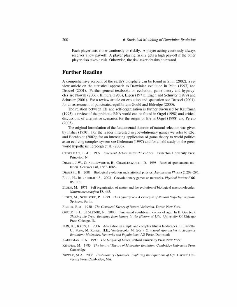
200 6 Statistical Modeling of Darwinian Evolution
Each player acts either cautiously or riskily. A player acting cautiously alwaysreceives a low pay-off. A player playing riskily gets a high pay-off if the otherplayer also takes a risk. Otherwise, the risk-taker obtains no reward.
Further ReadingA comprehensive account of the earth’s biosphere can be found in Smil (2002); a re-view article on the statistical approach to Darwinian evolution in Peliti (1997) andDrossel (2001). Further general textbooks on evolution, game-theory and hypercy-cles are Nowak (2006), Kimura (1983), Eigen (1971), Eigen and Schuster (1979) andSchuster (2001). For a review article on evolution and speciation see Drossel (2001),for an assessment of punctuated equilibrium Gould and Eldredge (2000).
The relation between life and self-organization is further discussed by Kauffman(1993), a review of the prebiotic RNA world can be found in Orgel (1998) and criticaldiscussions of alternative scenarios for the origin of life in Orgel (1998) and Pereto(2005).
The original formulation of the fundamental theorem of natural selection was givenby Fisher (1930). For the reader interested in coevolutionary games we refer to Ebeland Bornholdt (2002); for an interesting application of game theory to world politicsas an evolving complex system see Cederman (1997) and for a field study on the greenworld hypothesis Terborgh et al. (2006).
CEDERMAN, L.-E. 1997 Emergent Actors in World Politics. Princeton University PressPrinceton, N.
DRAKE, J.W., CHARLESWORTH, B., CHARLESWORTH, D. 1998 Rates of spontaneous mu-tation. Genetics 148, 1667–1686.
DROSSEL, B. 2001 Biological evolution and statistical physics. Advances in Physics 2, 209–295.
EBEL, H., BORNHOLDT, S. 2002 Coevolutionary games on networks. Physical Review E 66,056118.
EIGEN, M. 1971 Self organization of matter and the evolution of biological macromolecules.Naturwissenschaften 58, 465.
EIGEN, M., SCHUSTER, P. 1979 The Hypercycle – A Principle of Natural Self-Organization.Springer, Berlin.
FISHER, R.A. 1930 The Genetical Theory of Natural Selection. Dover, New York.
GOULD, S.J., ELDREDGE, N. 2000 Punctuated equilibrium comes of age. In H. Gee (ed),Shaking the Tree: Readings from Nature in the History of Life. University Of ChicagoPress Chicago, IL.
JAIN, K., KRUG, J. 2006 Adaptation in simple and complex fitness landscapes. In Bastolla,U., Porto, M, Roman, H.E., Vendruscolo, M. (eds.) Structural Approaches to SequenceEvolution: Molecules, Networks and Populations. AG Porto, Darmstadt
KAUFFMAN, S.A. 1993 The Origins of Order. Oxford University Press New York.
KIMURA, M. 1983 The Neutral Theory of Molecular Evolution. Cambridge University PressCambridge.
NOWAK, M.A. 2006 Evolutionary Dynamics: Exploring the Equations of Life. Harvard Uni-versity Press Cambridge, MA.

Further Reading 201
ORGEL, L.E 1998 The origin of life: A review of facts and speculations. Trends in Biochem-ical Sciences 23, 491–495.
PELITI, L. 1997 Introduction to the Statistical Theory of Darwinian Evolution. ArXiv preprintcond-mat/9712027.
PERETO, J. 2005 Controversies on the origin of life. International Microbiology 8, 23–31.
SCHUSTER, H.G. 2001 Complex Adaptive Systems – An Introduction. Scator, Saarbrucken.
SCHWEITZER, F., BEHERA, L., MUHLENBEIN, H. 2002 Evolution of cooperation in a spa-tial prisoner’s dilemma. Advances in Complex Systems 5, 269–299.
SMIL, V. 2002 The Earth’s Biosphere: Evolution, Dynamics, and Change. MIT Press,Cambridge, MA.
TERBORGH, J., FEELEY, K., SILMAN, M., NUNEZ, P., BALUKJIAN, B. 2006 Vegetationdynamics of predator-free land-bridge islands. Journal of Ecology 94, 253–263.

202 6 Statistical Modeling of Darwinian Evolution

Chapter 7
Synchronization Phenomena
Here we consider the dynamics of complex systems constituted of interacting localcomputational units that have their own non-trivial dynamics. An example for a localdynamical system is the time evolution of an infectious disease in a certain city thatis weakly influenced by an ongoing outbreak of the same disease in another city; orthe case of a neuron in a state where it fires spontaneously under the influence of theafferent axon potentials.
A fundamental question is then whether the time evolutions of these local units willremain dynamically independent of each other or whether, at some point, they will startto change their states all in the same rhythm. This is the notion of “synchronization”,which we will study throughout this chapter, learning that the synchronization pro-cess may be driven either by averaging dynamical variables or through causal mutualinfluences.
7.1 Frequency LockingIn this chapter we will be dealing mostly with autonomous dynamical systems whichmay synchronize spontaneously. A dynamical system may also be driven by outsideinfluences, being forced to follow the external signal synchronously.
The Driven Harmonic Oscillator As an example we consider the driven harmonicoscillator
x + γ x + ω20 x = F
(eiωt + c.c.
), γ > 0 . (7.1)
In the absence of external driving, F ≡ 0, the solution is
x(t) ∼ eλ t , λ ± =−γ
2±√
γ2
4−ω2
0 , (7.2)
which is damped/critical/overdamped for γ < 2ω0, γ = 2ω0 and γ > 2ω0.
Frequency Locking In the long time limit, t→∞, the dynamics of the system followsthe external driving, for all F 6= 0, due the damping γ > 0. We therefore consider the
203

204 CHAPTER 7. SYNCHRONIZATION PHENOMENA
ansatzx(t) = aeiωt + c.c., (7.3)
where the amplitude a may contain an additional time-independent phase. Using thisansatz for Eq. (7.1) we obtain
F = a(−ω
2 + iωγ +ω20)
= −a(ω
2− iωγ−ω20)= −a(ω + iλ+)(ω + iλ−) ,
where the eigenfrequencies λ± are given by Eq. (7.2). The solution for the amplitudea can then be written in terms of λ± or alternatively as
a =−F(
ω2−ω20
)− iωγ
. (7.4)
The response becomes divergent, viz a→ ∞, at resonance ω = ω0 and small dampingγ → 0.
The General Solution The driven, damped harmonic oscillator Eq. (7.1) is an inho-mogeneous linear differential equation and its general solution is given by the super-position of the special solution Eq. (7.4) with the general solution of the homogeneoussystem Eq. (7.2). The latter dies out for t → ∞ and the system synchronizes with theexternal driving frequency ω .
7.2 Synchronization of Coupled OscillatorsAny set of local dynamical systems may synchronize, whenever their dynamical be-haviours are similary and the mutual couplings substantial. We start by discussing thesimplest non-trivial set-up, viz harmonically coupled harmonic oscillators.Limiting Cycles A free rotation
~x(t) = r(
cos(ωt +φ0),sin(ωt +φ0)), θ(t) = ωt +θ0, θ = ω
often occurs (in suitable coordinates) as limiting cycles of dynamical systems, seeChap. 2. One can then use the phase variable θ(t) for an effective description.
Coupled Dynamical Systems We consider a collection of individual dynamical sys-tems i = 1, . . . ,N, which have limiting cycles with natural frequencies ωi. The coupledsystem then obeys
θi = ωi +N
∑j=1
Γi j(θi,θ j), i = 1, . . . ,N , (7.5)
where the Γi j are suitable coupling constants.
The Kuramoto Model A particularly tractable choice for the coupling constants Γi jhas been proposed by Kuramoto:
Γi j(θi,θ j) =KN
sin(θ j−θi) , (7.6)

7.2. SYNCHRONIZATION OF COUPLED OSCILLATORS 205
0 5 10 15 200
0.5
1
1.5
2
2.5
∆ω = 1.0 K = 0.9
K = 1.01
t
∆θ/π
Figure 7.1: The relative phase ∆θ(t) of two coupled oscillators, obeying Eq. (7.7), with∆ω = 1 and a critical coupling strength Kc = 1. For an undercritical coupling strengthK = 0.9 the relative phase increases steadily, for an overcritical coupling K = 1.01 itlocks
where K ≥ 0 is the coupling strength and the factor 1/N ensures that the model is wellbehaved in the limit N→ ∞.
Two Coupled Oscillators We consider first the case N = 2:
θ1 = ω1 +K2
sin(θ2−θ1), θ2 = ω2 +K2
sin(θ1−θ2) ,
or∆θ = ∆ω − K sin(∆θ), ∆θ = θ2−θ1, ∆ω = ω2−ω1 . (7.7)
The system has a fixpoint ∆θ ∗ for which
ddt
∆θ∗ = 0, sin(∆θ
∗) =∆ω
K(7.8)
and therefore∆θ∗ ∈ [−π/2,π/2], K > |∆ω| . (7.9)
This condition is valid for attractive coupling constants K > 0. For repulsive K < 0 anti-phase states are stabilized. We analyze the stability of the fixpoint using ∆θ = ∆θ ∗+δ
and Eq. (7.7). We obtain
ddt
δ = −(K cos∆θ∗) δ , δ (t) = δ0 e−K cos∆θ∗t .
The fixpoint is stable since K > 0 and cos∆θ ∗ > 0, due to Eq. (7.9). We thereforehave a bifurcation.
– For K < |∆ω| there is no phase coherence between the two oscillators, they aredrifting with respect to each other.
– For K > |∆ω| there is phase locking and the two oscillators rotate together witha constant phase difference.

206 CHAPTER 7. SYNCHRONIZATION PHENOMENA
This situation is illustrated in Fig. 7.1.
Natural Frequency Distribution We now consider the case of many coupled oscil-lators, N→ ∞. The individual systems have different individual frequencies ωi with aprobability distribution
g(ω) = g(−ω),∫
∞
−∞
g(ω)dω = 1 . (7.10)
We note that the choice of a zero average frequency∫∞
−∞
ω g(ω)dω = 0
implicit in Eq. (7.10) is actually generally possible, as the dynamical equations (7.5)and (7.6) are invariant under a global translation
ω → ω +Ω, θi → θi +Ωt ,
with Ω being the initial non-zero mean frequency.
The Order Parameter The complex order parameter
r eiψ =1N
N
∑j=1
eiθ j (7.11)
is a macroscopic quantity that can be interpreted as the collective rhythm produced bythe assembly of the interacting oscillating systems. The radius r(t) measures the degreeof phase coherence and ψ(t) corresponds to the average phase.
Molecular Field Representation We rewrite the order parameter definitionEq. (7.11) as
r ei(ψ−θi) =1N
N
∑j=1
ei(θ j−θi), r sin(ψ−θi) =1N
N
∑j=1
sin(θ j−θi) ,
retaining the imaginary component of the first term. Inserting the second expressioninto the governing equation (7.5) we find
θi = ωi +KN ∑
jsin(θ j−θi) = ωi + Kr sin(ψ−θi) . (7.12)
The motion of every individual oscillator i = 1, . . . ,N is coupled to the other oscillatorsonly through the mean-field phase ψ; the coupling strength being proportional to themean-field amplitude r.
The individual phases θi are drawn towards the self-consistently determined meanphase ψ , as can be seen in the numerical simulations presented in Fig. 7.2. Mean-fieldtheory is exact for the Kuramoto model. It is nevertheless non-trivial to solve, as theself-consistency condition (7.11) needs to be fulfilled.

7.2. SYNCHRONIZATION OF COUPLED OSCILLATORS 207
Figure 7.2: Spontaneous synchronization in a network of limit cycle oscillators withdistributed individual frequencies. Color coding: slowest (red)–fastest (violet) naturalfrequency. With respect to Eq. (7.5) an additional distribution of individual radii ri(t)has been assumed, the asterisk denotes the mean field reiψ = ∑i rieiθi/N, compareEq. (7.11), and the individual radii ri(t) are slowly relaxing (from Strogatz, 2001)
The Rotating Frame of Reference The order parameter reiψ performs a free rotationin the thermodynamic limit,
r(t) → r, ψ(t) → Ωt, N → ∞ ,
and one can transform via
θi → θi +ψ = θi +Ωt, θi → θi +Ω, ωi → ω +Ω
to the rotating frame of reference. The governing equation (7.12) then becomes
θi = ωi − Kr sin(θi) . (7.13)
This expression is identical to the one for the case of two coupled oscillators, Eq. (7.7),when substituting Kr by K. It then follows directly that ωi = Kr constitutes a specialpoint.
Drifting and Locked Components Equation (7.13) has a fixpoint θ ∗i for which θ ∗i =0 and
Kr sin(θ ∗i ) = ωi, |ωi| < Kr, θ∗i ∈ [−π
2,
π
2] . (7.14)
θ ∗i = 0 in the rotating frame of reference means that the participating limit cycles os-cillate with the average frequency ψ; they are “locked” to ψ , see Figs. 7.2 and 7.3.

208 CHAPTER 7. SYNCHRONIZATION PHENOMENA
−Kr
locked
Kr0 ω
drifingdrifting
Figure 7.3: The region of locked and drifting natural frequencies ωi → ω within theKuramoto model
For |ωi| > Kr the participating limit cycle drifts, i.e. θi never vanishes. They do,however, slow down when they approach the locked oscillators, see Eq. (7.13) andFig. 7.1.Stationary Frequency Distribution We denote by
ρ(θ ,ω)dθ
the fraction of drifting oscillators with natural frequency ω that lie between θ andθ +dθ . It obeys the continuity equation
∂ρ
∂ t+
∂
∂θ
(ρ θ
)= 0 ,
where ρθ is the respective current density. In the stationary case, ρ = 0, the stationaryfrequency distribution ρ(θ ,ω) needs to be inversely proportional to the speed
θ = ω − Kr sin(θ) .
The oscillators pile up at slow places and thin out at fast places on the circle. Hence
ρ(θ ,ω) =C
|ω−Kr sin(θ)|,
∫π
−π
ρ(θ ,ω)dθ = 1 , (7.15)
for ω > 0, where C is an appropriate normalization constant.Formulation of the Self-Consistency Condition We write the self-consistency con-dition (7.11) as
〈eiθ 〉 = 〈eiθ 〉locked + 〈eiθ 〉drifting = r eiψ ≡ r , (7.16)
where the brackets 〈·〉 denote population averages and where we have used the fact thatwe can set the average phase ψ to zero.Locked Contribution The locked contribution is
〈eiθ 〉locked =∫ Kr
−Kreiθ∗(ω)g(ω)dω =
∫ Kr
−Krcos((θ ∗(ω)) g(ω)dω ,
where we have assumed g(ω) = g(−ω) for the distribution g(ω) of the natural fre-quencies within the rotating frame of reference. Using Eq. (7.14),
dω = Kr cosθ∗ dθ
∗ ,
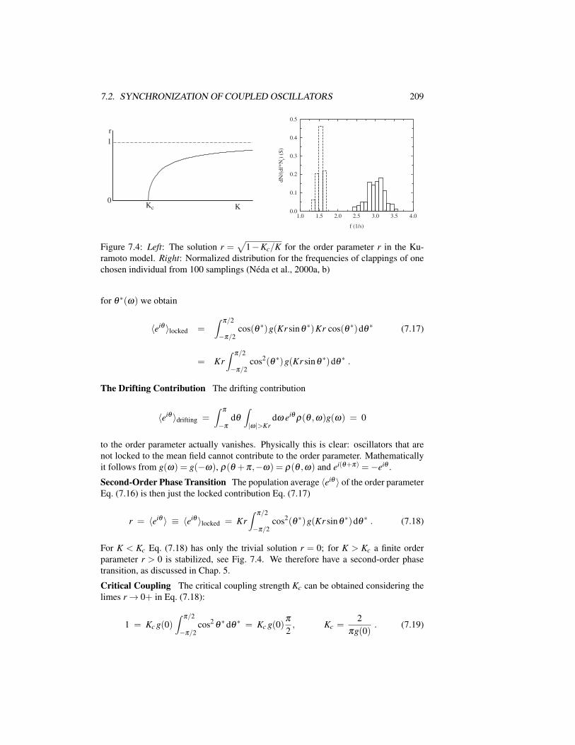
7.2. SYNCHRONIZATION OF COUPLED OSCILLATORS 209
K
1.00.0
0.1
0.2
0.3
0.4
0.5
1.5 2.0 2.5
f (1/s)
dN
/(df*
Nt)
(S
)
3.0 3.5 4.0
Kc
0
1
r
Figure 7.4: Left: The solution r =√
1−Kc/K for the order parameter r in the Ku-ramoto model. Right: Normalized distribution for the frequencies of clappings of onechosen individual from 100 samplings (Neda et al., 2000a, b)
for θ ∗(ω) we obtain
〈eiθ 〉locked =∫
π/2
−π/2cos(θ ∗)g(Kr sinθ
∗)Kr cos(θ ∗)dθ∗ (7.17)
= Kr∫
π/2
−π/2cos2(θ ∗)g(Kr sinθ
∗)dθ∗ .
The Drifting Contribution The drifting contribution
〈eiθ 〉drifting =∫
π
−π
dθ
∫|ω|>Kr
dω eiθρ(θ ,ω)g(ω) = 0
to the order parameter actually vanishes. Physically this is clear: oscillators that arenot locked to the mean field cannot contribute to the order parameter. Mathematicallyit follows from g(ω) = g(−ω), ρ(θ +π,−ω) = ρ(θ ,ω) and ei(θ+π) =−eiθ .
Second-Order Phase Transition The population average 〈eiθ 〉 of the order parameterEq. (7.16) is then just the locked contribution Eq. (7.17)
r = 〈eiθ 〉 ≡ 〈eiθ 〉locked = Kr∫
π/2
−π/2cos2(θ ∗)g(Kr sinθ
∗)dθ∗ . (7.18)
For K < Kc Eq. (7.18) has only the trivial solution r = 0; for K > Kc a finite orderparameter r > 0 is stabilized, see Fig. 7.4. We therefore have a second-order phasetransition, as discussed in Chap. 5.
Critical Coupling The critical coupling strength Kc can be obtained considering thelimes r→ 0+ in Eq. (7.18):
1 = Kc g(0)∫
π/2
−π/2cos2
θ∗ dθ
∗ = Kc g(0)π
2, Kc =
2πg(0)
. (7.19)

210 CHAPTER 7. SYNCHRONIZATION PHENOMENA
The self-consistency condition Eq. (7.18) can actually be solved exactly with the result
r =
√1− Kc
K, Kc =
2πg(0)
, (7.20)
as illustrated in Fig. 7.4.The Physics of Rhythmic Applause A nice application of the Kuramoto model isthe synchronization of the clapping of an audience after a performance, which happenswhen everybody claps at a slow frequency and in tact. In this case the distribution of“natural clapping frequencies” is quite narrow and K > Kc ∝ 1/g(0).
When an individual wants to express especial satisfaction with the performancehe/she increases the clapping frequency by about a factor of 2, as measured experimen-tally, in order to increase the noise level, which just depends on the clapping frequency.Measurements have shown, see Fig. 7.4, that the distribution of natural clapping fre-quencies is broader when the clapping is fast. This leads to a drop in g(0) and thenK < Kc ∝ 1/g(0). No synchronization is possible when the applause is intense.
7.3 Synchronization with Time DelaysSynchronization phenomena need the exchange of signals from one subsystem to an-other and this information exchange typically needs a certain time. These time delaysbecome important when they are comparable to the intrinsic time scales of the indi-vidual subsystems. A short introduction into the intricacies of time-delayed dynamicalsystems has been given in Sect. 2.6, here we discuss the effect of time delays on thesynchronization process.The Kuramoto Model with Time Delays We start with two limiting-cycle oscilla-tors, coupled via a time delay T :
θ1(t) = ω1 +K2
sin[θ2(t−T )−θ1(t)], θ2(t) = ω2 +K2
sin[θ1(t−T )−θ2(t)] .
In the steady state,
θ1(t) = ω t, θ2(t) = ω t + ∆θ∗ , (7.21)
there is a synchronous oscillation with a yet to be determined locking frequency ω anda phase slip ∆θ ∗. Using sin(α +β ) = sin(α)cos(β )+ cos(α)sin(β ) we find
ω = ω1 +K2[− sin(ωT )cos(∆θ
∗)+ cos(ωT )sin(∆θ∗)], (7.22)
ω = ω2 +K2[− sin(ωT )cos(∆θ
∗)− cos(ωT )sin(∆θ∗)].
Taking the difference we obtain
∆ω = ω2−ω1 = K sin(∆θ∗)cos(ωT ) , (7.23)
which generalizes Eq. (7.8) to the case of a finite time delay T . Eqs. (7.22) and (7.23)then determine together locking frequency ω and the phase slip ∆θ ∗.

7.3. SYNCHRONIZATION WITH TIME DELAYS 211
0 0.5 1 1.5ω
0
0.5
1
1.5
2ω
1-0.9*sin(ω)1-0.9*sin(6ω)
1
2
3
4
5
Figure 7.5: Left: Graphical solution of the self-consistency condition (7.24), given bythe intersections of the solid line with the dashed lines, for the locking frequency ω , andtime delays T = 1 (one solution) and T = 6 (three solutions in the inteval ω ∈ [0,1.5]).The coupling constant is K = 1.8. Right: An example of a directed ring, containingfive sites
Multiple Synchronization Frequencies For finite time delays T , there are generallymore than one solution for the synchronization frequency ω . For concreteness weconsider now the case
ω1 = ω2 ≡ 1, ∆θ∗ ≡ 0, ω = 1− K
2sin(ωT ) , (7.24)
compare Eqs. (7.23) and (7.22). This equation can be solved graphically, see Fig. 7.5.For T → 0 the two oscillators are phase locked, oscillating with the original natural
frequency ω = 1. A finite time delay then leads to a change of the synchronizationfrequency and eventually, for large enough time delay T and couplings K, to multiplesolutions for the locking frequency. These solutions are stable for
K cos(ωT ) > 0 ; (7.25)
we leave the derivation as an exercise to the reader. The time delay such results in aqualitative change in the structure of the phase space.Rings of Delayed-Coupled Oscillators As an example of the possible complexityarising from delayed couplings we consider a ring of N oscillators, as illustrated inFig. 7.5, coupled unidirectionally,
θ j = ω j + K sin[θ j−1(t−T )−θ j(t)], j = 1, ..,N . (7.26)
The periodic boundary conditions imply that N +1=1 in Eq. (7.26). We specialize tothe uniform case ω j ≡ 1. The network is then invariant under rotations of multiples of2π/N.
We consider plane-wave solutions1 with frequency ω and momentum k,
θ j = ω t − k j, k = nk2π
N, nk = 0, ..,N−1 , (7.27)
1In the complex plane ψ j(t) = eiθ j(t) = ei(ωt−k j) corresponds to a plane wave on a periodic ring.Eq. (7.26) is then equivalent to the phase evolution of the wavefunction ψ j(t). The system is invariant undertranslations j→ j+ 1 and the discrete momentum k is therefore a good quantum number, in the jargon ofquantum mechanics. The periodic boundary condition ψ j+N = ψ j is satisfied for the momenta k = 2πnk/N.

212 CHAPTER 7. SYNCHRONIZATION PHENOMENA
where j = 1, ..,N. For N = 2 only in-phase k = 0 and anti-phase k = π solutions exist.The locking frequency ω is then determined by the self-consistency condition
ω = 1 + K sin(k−ωT ) . (7.28)
For a given momentum k a set of solutions is obtained. The resulting solutions θ j(t) arecharacterized by complex spatio-temporal symmetries, oscillating fully in phase onlyfor vanishing momentum k→ 0. Note however, that additional unlocked solutions can-not be excluded and may show up in numerical solutions. It is important to rememberin this context, as discussed in Sect. 2.6, that initial conditions in the entire intervalt ∈ [−T,0] need to be provided.
7.4 Synchronization via Aggregate AveragingThe synchronization of the limiting cycle oscillators discussed in Sect. 7.2 is mediatedby the molecular field, which is an averaged quantity. Averaging plays a central role inmany synchronization processes and may act both on a local basis and on a global level.Alternatively, synchronization may be driven by the casual influence of temporally welldefined events, a route to synchronization we will discuss in Sect. 7.5.Pairwise Averaging The coupling term of the Kuramoto model, see Eq. (7.6), con-tains differences θi− θ j in the respective dynamical variables θi and θ j. With an ap-propriate sign of the coupling constant, this coupling results in a driving force towardsthe average,
θ1 →θ1 +θ2
2, θ2 →
θ1 +θ2
2.
This driving force competes with the differences in the time-development of the indi-vidual oscillators, which is present whenever their natural frequencies ωi and ω j donot coincide. A detailed analysis is then necessary, as carrried out in Sect. 7.2, in or-der to study this competion between the synchronizing effect of the coupling and thedesynchronizing influence of a non-trivial natural frequency distribution.Aggregate Variables Generalizing above considerations we consider now a set ofdynamical variables xi, with xi = fi(xi) being the evolution rule for the isolated units.The geometry of the couplings is given by the normalized weighted adjacency matrix
Ai j, ∑j
Ai j = 1 .
The matrix elements are Ai j > 0 if the units i and j are coupled, and zero otherwise,compare Chap. 1, with Ai j representing the relative weight of the link. We define nowthe aggregate variables xi = xi(t) by
xi = (1−κi)xi + κi ∑j
Ai jx j , (7.29)
where κi ∈ [0,1] is the local coupling strength. The aggregate variables xi correspondto a superposition of xi with the weighted mean activtiy ∑ j Ai jx j of all its neighbors.

7.4. SYNCHRONIZATION VIA AGGREGATE AVERAGING 213
Coupling via Aggregate Averaging A quite general class of dynamical networks cannow be formulated in terms of aggregate variables through
xi = fi(xi), i = 1, . . . , N , (7.30)
with the xi given by Eq. (7.29). The fi describe the local dynamical systems whichcould be, e.g., harmonic oscillators, relaxation oscillators or chaotic systems.
Expansion around the Synchronized State In order to expand Eq. (7.30) around theglobally synchronized state we first rewrite the aggregate variables as
xi = (1−κi)xi + κi ∑j
Ai j(x j− xi + xi) (7.31)
= xi
(1−κi +κi ∑
jAi j
)+κi ∑
jAi j(x j− xi) = xi + κi ∑
jAi j(x j− xi) ,
where we have used the normalization ∑ j Ai j = 1. The differences in activies x j− xiare small close to the synchronized state and we may expand
fi(xi) ≈ fi(xi) + f ′i (xi)κi ∑j
Ai j(x j− xi) . (7.32)
Differential couplings ∼ (x j− xi) between the nodes of the network are hence equiva-lent, close to synchronization, to the aggregate averaging of the local dynamics via therespective xi.
General Coupling Functions We may go one step further and define with
xi = f (xi) + ∑j
gi j(x j− xi) (7.33)
a general system of i = 1, . . . , N dynamical units interacting via the coupling functionsgi j(x j− xi). Close to the synchronized state we may expand Eq. (7.33) as
xi ≈ f (xi) + ∑j
g′i j(0)(x j− xi), g′i j(0) = f ′i (xi)κiAi j . (7.34)
The equivalence of g′i j(0) and f ′i (xi)κiAi j is only local in time, with the later being timedependent, but this equivalence is sufficient for a local stability analysis; the synchro-nized state of the system with differential couplings, Eq. (7.33), is locally stable thenand only then if the corresponding system with aggregate couplings, Eq. (7.30), is alsostable against perturbations.
Synchronization via Aggregated Averaging The equivalence of Eqs. (7.30) and(7.33) tells us that the driving forces leading to synchronization are aggregated averag-ing processes of neighboring dynamical variables.
Till now we considered globally synchronized states. Synchronization processesare however in general quite intricate processes, we mention here two alternative pos-sibilities. Above discussion concerning aggregate averaging remains however valid,when generalized suitably, also for these more generic synchronized states.

214 CHAPTER 7. SYNCHRONIZATION PHENOMENA
– We saw, when discussing the Kuramoto model in Sect. 7.2, that generically notall nodes of a network participate in a synchronization process. For the Kuramotomodel the oscillators with natural frequencies far away from the average do notbecome locked to the time development of the order parameter, see Fig. 7.3,retaining drifting trajectories.
– Generically, synchronization takes the form of coherent time evolution withphase lags, we have seen an example when discussing two coupled oscillatorsin Sect. 7.2. The synchronized orbit is then
xi(t) = x(t)+∆xi, ∆xi const. ,
viz the elements i = 1, . . . ,N are all locked in.
Stability Analysis via the Second-Largest Lyapunov Exponent The stability ofa globally synchronized state, xi(t) = x(t) for i = 1, . . . , N, can be determined byconsidering small perturbations, viz
xi(t) = x(t) + δi ct , |c|t = eλ t , (7.35)
where λ is the Lyapunov exponent. The eigenvectors (δ1, . . . , δN) of the perturbationare determined by the equation of motion linearized around the synchronized trajectory.There is one Lyapunov exponent for every eigenvector, N in all:
λ1 ≥ λ2 ≥ λ3 ≥ . . .≥ λN .
In general the largest eigenvector λ1 > 0 will correspond to the synchronized direction,
λ1, δi = δ , i = 1, . . . , N ,
corresponding to the dominant flow in phase space. The second largest Lyapunovexponent determines hence the stabilty of the synchronized orbit:
(λ2 < 0) ⇔ stability ,
and vice versa.
Coupled Logistic Maps As an example we consider two coupled logistic maps, seeFig. 2.5,
xi(t +1) = r xi(t)(1− xi(t)
), i = 1, 2, r ∈ [0,4] , (7.36)
withx1 = (1−κ)x1 +κx2, x2 = (1−κ)x2 +κx1
and κ ∈ [0,1] being the coupling strength. Using Eq. (7.35) as an Ansatz we obtain
c(
δ1δ2
)= r
(1−2x(t)
)( (1−κ) κ
κ (1−κ)
)(δ1δ2
),

7.5. SYNCHRONIZATION VIA CAUSAL SIGNALING 215
which determines c as the eigenvalues of the Jacobian of Eq. (7.36). We have hencetwo local pairs of eigenvalues and eigenvectors, namely
c1 = r(1−2x) (δ1,δ2) =1√2(1,1)
c2 = r(1−2x)(1−2κ) (δ1,δ2) =1√2(1,−1)
corresponding to the respective local Lyapunov exponents, λ = log |c|,
λ1 = log |r(1−2x)|, λ2 = log |r(1−2x)(1−2κ)| . (7.37)
As expected, λ1 > λ2, since λ1 corresponds to a perturbation along the synchronizedorbit. The overall stability of the synchronized trajectory can be examined by averagingabove local Lyapunov exponents over the full time development, obtaining such themaximal Lyapunov exponent, see Eq. (2.16).Synchronization of Coupled Chaotic Maps The maximal Lyapunov exponent needsto be evaluated numerically, but we can obtain an upper bound for the coupling strengthκ needed for stable synchronization by observing that |1−2x| ≤ 1 and hence
|c2| ≤ r|1−2κ| .
The synchronized orbit is stable for |c2|< 1. Considering the case κ ∈ [0,1/2] we find
1 > r(1−2κs) ≥ |c2|, κs >r−1
2r
for the upper bound for κs. The logistic map is chaotic for r > r∞ ≈ 3.57 and aboveresult, being valid for all r ∈ [0,4], therefore proves that also chaotic coupled systemsmay synchronize.
For the maximal reproduction rate, r = 4, synchronization is guaranteed for 3/8<κs ≤ 1/2. Note that x1 = x2 for κ = 1/2, synchronization through aggregate averagingis hence achieved in one step for κ = 1/2.
7.5 Synchronization via Causal SignalingThe synchronization of the limiting cycle oscillators discussed in Sect. 7.2 is very slow,see Fig. 7.2, as the information between the different oscillators is exchanged only in-directly via the molecular field, which is an averaged quantity. Synchronization may besustantially faster, when the local dynamical units influence each other with preciselytimed signals, the route to synchronization discussed here.
Relaxational oscillators, like the van der Pol oscillator discussed in Chap. 2 havea non-uniform cycle and the timing of the stimulation of one element by another isimportant. This is a characteristic property of real-world neurons in particular and ofmany models of artificial neurons, like the so-called integrate-and-fire models. Relax-ational oscillators are hence well suited to study the phenomena of synchronization viacausal signaling.

216 CHAPTER 7. SYNCHRONIZATION PHENOMENA
-2 1 2
x
0
4
8
y
-2 –1
dy/dt=0
dx/dt=0
relaxational state
I > 0
LB RB
–2 –1 2
x
0
4
8
y
dy/dt=0
dx/dt=0
PI
excitable state
I < 0
0 10
Figure 7.6: The y = 0 (thick dashed-dotted lines) and the x = 0 (thick full lines) isoclineof the Terman–Wang oscillator, Eq. (7.38), for α = 5, β = 0.2, ε = 0.1. Left: I = 0.5with the limiting relaxational cycle for ε 1 (thin dotted line with arrows). Right:I =−0.5 with the stable fixpoint: PI
Terman–Wang Oscillators There are many variants of relaxation oscillators relevantfor describing integrate-and-fire neurons, starting from the classical Hodgkin–Huxleyequations. Here we discuss the particularly transparent dynamical system introducedby Terman and Wang, namely
x = f (x)− y+ I
y = ε(g(x)− y
) f (x) = 3x− x3 +2
g(x) = α(1+ tanh(x/β )
) . (7.38)
Here x corresponds in neural terms to the membrane potential and I represents theexternal stimulation to the neural oscillator. The amount of dissipation is given by
∂ x∂x
+∂ y∂y
= 3−3x2− ε = 3(1− x2)− ε .
For small ε 1 the system takes up energy for membrane potentials |x|< 1 and dissi-pates energy for |x|> 1.
Fixpoints The fixpoints are determined via
x = 0y = 0
y = f (x)+ I
y = g(x)
by the intersection of the two functions f (x)+ I and g(x), see Fig. 7.6. We find twoparameter regimes:
– For I ≥ 0 we have one unstable fixpoint (x∗,y∗) with x∗ ' 0.
– For I < 0 and |I| large enough we have two additional fixpoints given by thecrossing of the sigmoid α
(1+ tanh(x/β )
)with the left branch (LB) of the cubic
f (x) = 3x− x3 +2, with one fixpoint being stable.

7.5. SYNCHRONIZATION VIA CAUSAL SIGNALING 217
0 20 40 60 80
time
–2
0
2
4
6x
(t),
y(t
)relaxationalI > 0
y(t)
x(t)
0 20 40 60 80
time
–2
0
2
4excitable stateI < 0
y(t)
x(t)
Figure 7.7: Sample trajectories y(t) (thick dashed-dotted lines) and x(t) (thick full lines)of the Terman–Wang oscillator Eq. (7.38) for α = 5, β = 0.2, ε = 0.1. Left: I = 0.5exhibiting spiking behavior, having silent/active phases for negative/positive x. Right:I =−0.5, relaxing to the stable fixpoint
The stable fixpoint PI is indicated in Fig. 7.6.
The Relaxational Regime For the case I > 0 the Terman–Wang oscillator relaxesin the long time limit to a periodic solution, see Fig. 7.6, which is very similar tothe limiting relaxation oscillation of the Van der Pol oscillator discussed inChap. 2.
Silent and Active Phases In its relaxational regime, the periodic solution jumps veryfast (for ε 1) between trajectories that approach closely the right branch (RB) andthe left branch (LB) of the x = 0 isocline. The time development on the RB and the LBare, however, not symmetric, see Figs. 7.6 and 7.7, and we can distinguish two regimes:
The Silent Phase. We call the relaxational dynamics close to the LB(x< 0) of the x = 0 isocline the silent phase or the refractory period.
The Active Phase. We call the relaxational dynamics close to the RB(x> 0) of the x = 0 isocline the active phase.
The relative rate of the time development y in the silent and active phases are deter-mined by the parameter α , compare Eq. (7.38).
The active phase on the RB is far from the y = 0 isocline for α 1, see Fig. 7.6,and the time development y is then fast. The silent phase on the LB is, however, alwaysclose to the y = 0 isocline and the system spends considerable time there.
The Spontaneously Spiking State and the Separation of Time Scales In its re-laxational phase, the Terman–Wang oscillator can therefore be considered as a spon-taneously spiking neuron, see Fig. 7.7, with the spike corresponding to the active phase,which might be quite short compared to the silent phase forα 1.
The Terman–Wang differential equations (7.38) are examples of a standard tech-nique within dynamical system theory, the coupling of a slow variable, y, to a fastvariable, x, which results in a separation of time scales. When the slow variable y(t)

218 CHAPTER 7. SYNCHRONIZATION PHENOMENA
RBE
LBE
LB
RB
o1(t2)
o2(t2)
o2(t)
o1(t)
o1(t1)
o2(t1)
o1(0)
o2(0)
x
y
−2 10 2
2
4
6
8
dy/dt = 0
C
CE
–1
Figure 7.8: Fast threshold modulation for two excitatory coupled Terman–Wang oscil-lators, Eq. (7.38) o1 = o1(t) and o2 = o2(t), which start at time 0. When o1 jumps att = t1 the cubic x = 0 isocline for o2 is raised from C to CE . This induces o2 to jumpas well. Note that the jumping from the right branches (RB and RBE ) back to the leftbranches occurs in the reverse order: o2 jumps first (from Wang, 1999)
relaxes below a certain threshold, see Fig. 7.7, the fast variable x(t) responds rapidlyand resets the slow variable. We will encounter further applications of this procedurein Chap. 8.The Excitable State The neuron has an additional phase with a stable fixpoint PI onthe LB (within the silent region), for negative external stimulation (suppression) I < 0.The dormant state at the fixpoint PI is “excitable”: A positive external stimulationabove a small threshold will force a transition into the active phase, with the neuronspiking continuously.Synchronization via Fast Threshold Modulation Limit cycle oscillators can syn-chronize, albeit slowly, via the common molecular field, as discussed in Sect. 7.2. Amuch faster synchronization can be achieved via fast threshold synchronization for anetwork of interacting relaxation oscillators.
The idea is simple. Relaxational oscillators have distinct states during their cy-cle; we called them the “silent phase” and the “active phase” for the case of theTerman–Wang oscillator. We then assume that a neural oscillator in its (short) activephase changes the threshold I of the other neural oscillator in Eq. 7.38 as
I → I + ∆I, ∆I > 0 ,
such that the second neural oscillator changes from an excitable state to the oscillatingstate. This process is illustrated graphically in Fig. 7.8; it corresponds to a signal sendfrom the first to the second dynamical unit. In neural terms: when the first neuron fires,the second neuron follows suit.Propagation of Activity We consider a simple model

7.6. SYNCHRONIZATION AND OBJECT RECOGNITION IN NEURAL NETWORKS219
0 50 100 150
time
–3
–2
–1
0
1
2
xi(t)
i = 1,2,3,4,5
∆I1(t)
Figure 7.9: Sample trajectories xi(t) (lines) for a line of coupled Terman–Wang oscil-lators, an example of synchronization via causal signaling. The relaxational oscillatorsare in excitable states, see Eq. (7.38), with α = 10, β = 0.2, ε= 0.1 and I =−0.5. Fort ∈ [20,100] a driving current ∆I1 = 1 is added to the first oscillator. x1 then starts tospike, driving the other oscillators one by one via a fast threshold modulation.
1 ⇒ 2 ⇒ 3 ⇒ . . .of i = 1, . . . ,N coupled oscillators xi(t), yi(t), all being initially in the excitable statewith Ii ≡−0.5. They are coupled via fast threshold modulation, specifically via
∆Ii(t) = Θ(xi−1(t)) , (7.39)
where Θ(x) is the Heaviside step function. That is, we define an oscillator i to be in itsactive phase whenever xi > 0. The resulting dynamics is shown in Fig. 7.9. The chainis driven by setting the first oscillator of the chain into the spiking state for a certainperiod of time. All other oscillators start to spike consecutively in rapid sequence.
7.6 Synchronization and Object Recognitionin Neural Networks
Synchronization phenomena can be observed in many realms of the living world. Asan example we discuss here the hypothesis of object definition via synchronous neuralfiring, a proposal by Singer and von der Malsburg which is at the same time bothfascinating and controversial.Temporal Correlation Theory The neurons in the brain have time-dependent ac-tivities and can be described by generalized relaxation oscillators, as outlined in theprevious Section. The “temporal correlation theory” assumes that not only the averageactivities of individual neurons (the spiking rate) are important, but also the relativephasing of the individual spikes. Indeed, experimental evidence supports the notionof object definition in the visual cortex via synchronized firing. In this view neuronsencoding the individual constituent parts of an object, like the mouth and the eyes of a

220 CHAPTER 7. SYNCHRONIZATION PHENOMENA
face, fire in tact. Neurons being activated simultaneously by other objects in the visualfield, like a camera, would fire independently.
The LEGION Network of Coupled Relaxation Oscillators As an example of howobject definition via coupled relaxation oscillators can be achieved we consider theLEGION (local excitatory globally inhibitory oscillator network) network by Termanand Wang. Each oscillator i is defined as
xi = f (xi)− yi + Ii +Si +ρ
yi = ε(g(xi)− yi
) f (x) = 3x− x3 +2g(x) = α
(1+ tanh(x/β )
) . (7.40)
There are two terms in addition to the ones necessary for the description of a singleoscillator, compare Eq. (7.38):
ρ : a random-noise term andSi : the interneural interaction.
The interneural coupling in Eq. (7.40) occurs exclusively via the modulation of thethreshold, the three terms Ii +Si +ρ constitute an effective threshold.
Interneural Interaction The interneural interaction is given for the LEGION networkby
Si = ∑l∈N(i)
Til Θ(xl− xc) −WzΘ(z− zc) , (7.41)
where Θ(z) is the Heaviside step function. The parameters have the following meaning:Til > 0 : Interneural excitatory couplings.
N(i) : Neighborhood of neuron i.xc : Threshold determining the active phase.z : Variable for the global inhibitor.
−Wz < 0 : Coupling to the global inhibitor z.zc : Threshold for the global inhibitor.
Global Inhibition Global inhibition is a quite generic strategy for neural networkswith selective gating capabilities. A long-range or global inhibition term assures thatonly one or only a few of the local computational units are active coinstantaneously. Inthe context of the Terman–Wang LEGION network it is assumed to have the dynamics
z = (σz− z)φ , φ > 0 , (7.42)
where the binary variable σz is determined by the following rule:
σz = 1 if at least one oscillator is active.
σz = 0 if all oscillators are silent or in the excitable state.
This rule is very non-biological, the LEGION network is just a proof of the prin-ciple for object definition via fast synchronization. When at least one oscillator is inits active phase the global inhibitor is activated, z→ 1, and inhibition is turned offwhenever the network is completely inactive.
Simulation of the LEGION Network A simulation of a 20×20 LEGION networkis presented in Fig. 7.10. We observe the following:

7.6. SYNCHRONIZATION AND OBJECT RECOGNITION IN NEURAL NETWORKS221
(a) (b) (c)
(f)(e)(d)
(g)
Left O
Pattern H
Pattern I
RightO
Inhibitor
Time
Figure 7.10: (a) A pattern used to stimulate a 20× 20 LEGION network. (b) Initialrandom activities of the relaxation oscillators. (c, d, e, f) Snapshots of the activities atdifferent sequential times. (g) The corresponding time-dependent activities of selectedoscillators and of the global inhibitor (from Wang, 1999)
– The network is able to discriminate between different input objects.
– Objects are characterized by the coherent activity of the corresponding neurons,while neurons not belonging to the active object are in the excitable state.
– Individual input objects pop up randomly one after the other.
Working Principles of the LEGION Network The working principles of the LE-GION network are the following:
– When the stimulus begins there will be a single oscillator k, which will jump firstinto the active phase, activating the global inhibitor, Eq. (7.42), via σz→ 1. Thenoise term ∼ ρ in Eq. (7.40) determines the first active unit randomly from theset of all units receiving an input signal ∼ Ii, whenever all input signals havethe same strength.
– The global inhibitor then suppresses the activity of all other oscillators, apartfrom the stimulated neighbors of k, which also jump into the active phase, havingset the parameters such that
I +Tik−Wz > 0, I : stimulus

222 CHAPTER 7. SYNCHRONIZATION PHENOMENA
is valid. The additional condition
I−Wz < 0
assures, that units receiving an input, but not being topologically connected tothe cluster of active units, are suppressed. No two distinct objects can then beactivated coinstantaneously.
– This process continues until all oscillators representing the stimulated patternare active. As this process is very fast, all active oscillators fire nearly simulta-neously, compare also Fig. 7.9.
– When all oscillators in a pattern oscillate in phase, they also jump back to thesilent state simultaneously. At that point the global inhibitor is turned off: σz→ 0in Eq. (7.42) and the game starts again with a different pattern.
Discussion Even though the network nicely performs its task of object recognitionvia coherent oscillatory firing, there are a few aspects worth noting:
– The functioning of the network depends on the global inhibitor triggered by thespecific oscillator that jumps first. This might be difficult to realize in biologicalnetworks, like the visual cortex, which do not have well defined boundaries.
– The first active oscillator sequentially recruits all other oscillators belonging toits pattern. This happens very fast via the mechanism of rapid threshold modula-tion. The synchronization is therefore not a collective process in which the inputdata is processed in parallel; a property assumed to be important for biologicalnetworks.
– The recognized pattern remains active for exactly one cycle and no longer.
We notice, however, that the design of neural networks capable of fast synchronizationvia a collective process remains a challenge, since collective processes have an inherenttendency towards slowness, due to the need to exchange information, e.g. via molecularfields. Without reciprocal information exchange, a true collective state, as an emergentproperty of the constituent dynamical units, is not possible.
7.7 Synchronization Phenomena in EpidemicsThere are illnesses, like measles, that come and go recurrently. Looking at the localstatistics of measle outbreaks, see Fig. 7.11, one can observe that outbreaks occur inquite regular time intervals within a given city. Interestingly though, these outbreakscan be either in phase (synchronized) or out of phase between different cities.
The oscillations in the number of infected persons are definitely not harmonic, theyshare many characteristics with relaxation oscillations, which typically have silent andactive phases, compare Sect. 7.5.The SIRS Model A standard approach to model the dynamics of infectious diseasesis the SIRS model. At any time an individual can belong to one of the three classes:

7.7. SYNCHRONIZATION PHENOMENA IN EPIDEMICS 223
0
0.5
1
44 46 48 50 52 54 56 58 0
0.5
1
years
(a)
(b)
wee
kly
mea
sle
case
s
Figure 7.11: Observation of the number of infected persons in a study on illnesses. (a)Weekly cases of measle cases in Birmingham (red line) and Newcastle (blue line). (b)Weekly cases of measle cases in Cambridge (green line) and in Norwich (pink line)(from He, 2003)
S : susceptible,I : infected,
R : recovered.
The dynamics is governed by the following rules:
(a) Susceptibles pass to the infected state, with a certain probability, after cominginto contact with one infected individual.
(b) Infected individuals pass to the recovered state after a fixed period of time τI .
(c) Recovered individuals return to the susceptible state after a recovery time τR,when immunity is lost, and the S→I→R→ S cycle is complete.
When τI → ∞ (lifelong immunity) the model reduces to the SIR-model.The Discrete Time Model We consider a discrete time SIRS model with t = 1,2,3, . . .and τI = 1: The infected phase is normally short and we can use it to set the unit oftime. The recovery time τR is then a multiple of τI = 1.We define with
xt the fraction of infected individuals at time t,st the percentage of susceptible individuals at time t,
which obey
st = 1− xt −τR
∑k=1
xt−k = 1−τR
∑k=0
xt−k , (7.43)
as the fraction of susceptible individuals is just 1 minus the number of infected indi-viduals minus the number of individuals in the recovery state, compare Fig. 7.12.

224 CHAPTER 7. SYNCHRONIZATION PHENOMENA
S S S I R R R S S State
1 Time98765432
Figure 7.12: Example of the course of an individual infection within the SIRS modelwith an infection time τI = 1 and a recovery time τR = 3. The number of individualsrecovering at time t is just the sum of infected individuals at times t−1, t−2 and t−3,compare Eq. (7.43)
The Recursion Relation We denote with a the rate of transmitting an infection whenthere is a contact between an infected individual and a susceptible individual:
xt+1 = axtst = axt
(1−
τR
∑k=0
xt−k
). (7.44)
Relation to the Logistic Map For τR = 0 the discrete time SIRS model (7.44)reduces to the logistic map
xt+1 = axt (1− xt) ,
which we studied in Chap. 2. For a< 1 it has only the trivial fixpoint xt ≡ 0, the illnessdies out. The non-trivial steady state is
x(1) = 1− 1a, for 1< a< 3 .
For a = 3 there is a Hopf bifurcation and for a > 3 the system oscillates with a periodof 2. Equation (7.44) has a similar behavior, but the resulting oscillations may dependon the initial condition and for τR τI ≡ 1 show features characteristic of relaxationoscillators, see Fig. 7.13.Two Coupled Epidemic Centers We consider now two epidemic centers with vari-ables
s(1,2)t , x(1,2)t ,
denoting the fraction of susceptible/infected individuals in the respective cities. Dif-ferent dynamical couplings are conceivable, via exchange or visits of susceptible orinfected individuals. We consider with
x(1)t+1 = a(
x(1)t + ex(2)t
)s(1)t , x(2)t+1 = a
(x(2)t + ex(1)t
)s(2)t (7.45)
the visit of a small fraction e of infected individuals to the other center. Equation (7.45)determines the time evolution of the epidemics together with Eq. (7.43), generalized toboth centers. For e = 1 there is no distinction between the two centers anymore andtheir dynamics can be merged via xt = x(1)t + x(2)t and st = s(1)t + s(2)t to the one of asingle center.In Phase Versus Out of Phase Synchronization We have seen in Sect. 7.2 that astrong coupling of relaxation oscillators during their active phase leads in a quite natu-ral way to a fast synchronization. Here the active phase corresponds to an outbreak of

7.7. SYNCHRONIZATION PHENOMENA IN EPIDEMICS 225
0 60 800
0.05
0.1
0.15
0.2
0.25
xt+1 = 2.2 xt (1–xt–xt–1–xt–2–xt–3–xt–4–xt–5–xt–6)
t1004020
Figure 7.13: Example of a solution to the SIRS model, Eq. (7.44), for τR = 6. Thenumber of infected individuals might drop to very low values during the silent phase inbetween two outbreaks as most of the population is first infected and then immunizedduring an outbreak
the illness and Eq. (7.45) indeed implements a coupling equivalent to the fast thresholdmodulation discussed in Sect. 7.5, since the coupling is proportional to the fraction ofinfected individuals.
In Fig. 7.14 we present the results from a numerical simulation of the coupledmodel, illustrating the typical behavior. We see that the outbreaks of epidemics in theSIRS model indeed occur in phase for a moderate to large coupling constant e. Forvery small coupling e between the two centers of epidemics on the other hand, thesynchronization becomes antiphase, as is sometimes observed in reality, see Fig. 7.11.
Time Scale Separation The reason for the occurrence of out of phase synchronizationis the emergence of two separate time scales in the limit tR 1 and e 1. A smallseed ∼ eax(1)s(2) of infections in the second city needs substantial time to induce afull-scale outbreak, even via exponential growth, when e is too small. But in order toremain in phase with the current outbreak in the first city the outbreak occurring inthe second city may not lag too far behind. When the dynamics is symmetric underexchange 1↔ 2 the system then settles in antiphase cycles.
ExercisesTHE DRIVEN HARMONIC OSCILLATOR
Solve the driven harmonic oscillator, Eq. (7.1), for all times t and compare itwith the long time solution t→ ∞, Eqs. (7.3) and (7.4).
SELF-SYNCHRONIZATION

226 CHAPTER 7. SYNCHRONIZATION PHENOMENA
0
0.1
0.2
0.3
xt(i)
xt(i)
a = 2, e = 0.005, τR = 6, x0(1)
= 0.01, x0(2)
= 0
a = 2, e = 0.100, τR = 6, x0(1)
= 0.01, x0(2)
= 0
t0 10 20 30 40 50 60
0
0.1
0.2
0.3
Figure 7.14: Time evolution of the fraction of infected individuals x(1)(t) and x(2)(t)within the SIRS model, Eq. (7.45), for two epidemic centers i = 1,2 with recoverytimes τR = 6 and infection rates a = 2, see Eq. (7.44). For a very weak couplinge = 0.005 (top) the outbreaks occur out of phase, for a moderate coupling e = 0.1(bottom) in phase
Consider an oscillator with feedback,
θ(t) = ω0 + K sin[θ(t−T )−θ(t)] .
Discuss the self-synchronization in analogy to Sect. 7.3, the stability of thesteady-state solutions and the auto-locking frequencies in the limit of strong self-coupling K→ ∞.
SYNCHRONIZATION OF CHAOTIC MAPS
The Bernoulli shift map f (x) = ax mod 1 with x ∈ [0,1] is chaotic for a > 1.Consider with
x1(t +1) = f((1−κ)x1(t)+κx2(t−T )
)x2(t +1) = f
((1−κ)x2(t)+κx1(t−T )
) (7.46)
two coupled chaotic maps, with κ ∈ [0,1] being the coupling strength and T thetime delay, compare Eq. (7.30). Discuss the stability of the synchronized statesx1(t) = x2(t)≡ x(t) for general time delays T . What drives the synchronizationprocess?
THE TERMAN–WANG OSCILLATOR
Discuss the stability of the fixpoints of the Terman–Wang oscillator, Eq. (7.38).Linearize the differential equations around the fixpoint solution and consider thelimit β → 0.
THE SIRS MODEL – ANALYTICAL

Further Reading 227
Find the fixpoints xt ≡ x∗ of the SIRS model, Eq. (7.44), for all τR, as a functionof a and study their stability for τR = 0,1.
THE SIRS MODEL – NUMERICAL
Study the SIRS model, Eq. (7.44), numerically for various parameters a andτR = 0,1,2,3. Try to reproduce Figs. 7.13 and 7.14.
Further ReadingA nice review of the Kuramoto model, together with historical annotations, has beenpublished by Strogatz (2000), for a textbook containing many examples of synchro-nization see Pikovsky et al. (2003). Some of the material discussed in this chapterrequires a certain background in theoretical neuroscience, see e.g. Dayan and Abbott(2001).
We recommend that the interested reader takes a look at some of the original re-search literature, such as the exact solution of the Kuramoto (1984) model, the Termanand Wang (1995) relaxation oscillators, the concept of fast threshold synchronization(Somers and Kopell, 1993), the temporal correlation hypothesis for cortical networks(von der Malsburg and Schneider, 1886), and its experimental studies (Gray et al.,1989), the LEGION network (Terman and Wang, 1995), the physics of synchronizedclapping (Neda et al., 2000a, b) and synchronization phenomena within the SIRS modelof epidemics (He and Stone, 2003). For an introductory-type article on synchronizationwith delays see (D’Huys et al, 2008).
DAYAN, P., ABBOTT, L.F. 2001 Theoretical Neuroscience: Computational and Mathemati-cal Modeling of Neural Systems. MIT Press, Cambridge.
D′HUYS, O.,VICENTE, R., ERNEUX, T., DANCKAERT, J., FISCHER, I. 2008 Synchroniza-tion properties of network motifs: Influence of coupling delay and symmetry. Chaos 18,037116.
GRAY, C.M., KONIG, P., ENGEL, A.K., SINGER, W. 1989 Oscillatory responses in cat vi-sual cortex exhibit incolumnar synchronization which reflects global stimulus properties.Nature 338, 334–337.
HE, D., STONE, L. 2003 Spatio-temporal synchronization of recurrent epidemics. Proceed-ings of the Royal Society London B 270, 1519–1526.
KURAMOTO, Y. 1984 Chemical Oscillations, Waves and Turbulence. Springer, Berlin.
NEDA, Z., RAVASZ, E., VICSEK, T., BRECHET, Y., BARABASI, A.L. 2000a Physics of therhythmic applause. Physical Review E 61, 6987–6992.
NEDA, Z., RAVASZ, E., VICSEK, T., BRECHET, Y., BARABASI, A.L. 2000b The sound ofmany hands clapping. Nature 403, 849–850.
PIKOVSKY, A., ROSENBLUM, M., KURTHS, J. 2003 Synchronization: A Universal Conceptin Nonlinear Sciences. Cambridge University Press.
SOMERS, D., KOPELL, N. 1993 Rapid synchronization through fast threshold modulation.Biological Cybernetics 68, 398–407.

228 7 Synchronization Phenomena
STROGATZ, S.H. 2000 From Kuramoto to Crawford: Exploring the onset of synchronizationin populations of coupled oscillators. Physica D 143, 1–20.
STROGATZ, S.H. 2001 Exploring complex networks. Nature 410, 268–276.
TERMAN, D., WANG, D.L. 1995 Global competition and local cooperation in a network ofneural oscillators. Physica D 81, 148–176.
VON DER MALSBURG, C., SCHNEIDER, W. 1886 A neural cocktail-party processor. Biolog-ical Cybernetics 54, 29–40.
WANG, D.L. 1999 Relaxation oscillators and networks. In Webster, J.G. (ed.) Encyclopediaof Electrical and Electronic Engineers, pp. 396–405, Wiley, New York.

Chapter 8
Elements of Cognitive SystemsTheoryThe brain is without doubt the most complex adaptive system known to humanity, ar-guably also a complex system about which we know very little.
Throughout this book we have considered and developed general guiding principlesfor the understanding of complex networks and their dynamical properties; principlesand concepts transcending the details of specific layouts realized in real-world complexsystems. We follow the same approach here, considering the brain as just one exampleof what is called a cognitive system, a specific instance of what one denotes, cum granosalis, a living dynamical system.
In the first part we will treat general layout considerations concerning dynamicalorganizational principles, an example being the role of diffuse controlling and home-ostasis for stable long-term cognitive information processing. Special emphasis willbe given to the motivational problem – how the cognitive system decides what to do –in terms of survival parameters of the living dynamical system and the so-called emo-tional diffusive control.
In the second part we will discuss two specific generalized neural networks imple-menting various aspects of these general principles: a dense and homogeneous asso-ciative network (dHAN) for environmental data representation and associative thoughtprocesses, and the simple recurrent network (SRN) for concept extraction from univer-sal prediction tasks.
8.1 IntroductionWe start with a few basic considerations concerning the general setting.What is a Cognitive System? A cognitive system may be either biological, likethe brain, or artificial. It is, in both instances, a dynamical system embedded into anenvironment, with which it mutually interacts.
Cognitive Systems. A cognitive system is a continuously active com-plex adaptive system autonomously exploring and reacting to the environ-ment with the capability to “survive”.
229

230 CHAPTER 8. ELEMENTS OF COGNITIVE SYSTEMS THEORY
sensory signals
survivial variables
cognitive
system
output signals − actions
environmentautonomous
dynamics
Figure 8.1: A cognitive system is placed in an environment (compare Sect. 8.2.4) fromwhich it receives two kinds of signals. The status of the survival parameters, whichit needs to regulate (see Sect. 8.3.2), and the standard sensory input. The cognitivesystem generates output signals via its autonomous dynamics, which act back onto theoutside world, viz the environment
For a cognitive system, the only information source about the outside is given, to beprecise, by its sensory data input stream, viz the changes in a subset of variables trig-gered by biophysical processes in the sensory organs or sensory units. The cognitivesystem does therefore not react directly to environmental events but to the resultingchanges in the sensory data input stream, compare Fig. 8.1.Living Dynamical Systems A cognitive system is an instance of a living dynam-ical system, being dependent on a functioning physical support unit, the body. Thecognitive system is terminated when its support unit ceases to work properly.
Living Dynamical Systems. A dynamical system is said to “live”in an abstract sense if it needs to keep the ongoing dynamical activity incertain parameter regimes.
As an example we consider a dynamical variable y(t) ≥ 0, part of the cognitive sys-tem, corresponding to the current amount of pain or hunger. This variable could bedirectly set by the physical support unit, i.e. the body, of the cognitive system, tellingthe dynamical system about the status of its support unit.
The cognitive system can influence the value of y(t) indirectly via its motor outputsignals, activating its actuators, e.g. the limbs. These actions will, in general, triggerchanges in the environment, like the uptake of food, which in turn will influence thevalues of the respective survival variables. One could then define the termination of thecognitive system when y(t) surpasses a certain threshold yc. The system “dies” wheny(t)> yc. These issues will be treated in depth in Sect. 8.3.2.Cognition Versus Intelligence A cognitive system is not necessarily intelligent, but itmight be in principle. Cognitive system theory presumes that artificial intelligence canbe achieved only once autonomous cognitive systems have been developed. This stanceis somewhat in contrast with the usual paradigm of artificial intelligence (AI), whichfollows an all-in-one-step approach to intelligentsystems.Universality Simple biological cognitive systems are dominated by cognitive capabil-ities and algorithms hard-wired by gene expression. These features range from simplestimulus–response reactions to sophisticated internal models for limb dynamics.

8.2. FOUNDATIONS OF COGNITIVE SYSTEMS THEORY 231
A priori information is clearly very useful for task solving in particular and for cog-nitive systems in general. A main research area in AI is therefore the development ofefficient algorithms making maximal use of a priori information about the environment.A soccer-playing robot normally does not acquire the ball dynamics from individual ex-perience. Newton’s law is given to the robot by its programmer and hard-wired withinits code lines.
Cognitive system theory examines, on the other hand, universal principles and al-gorithms necessary for the realization of an autonomous cognitive system. This chapterwill be devoted to the discussion and possible implementations of such universal prin-ciples.
A cognitive system should therefore be able to operate in a wide range of environ-mental conditions, performing tasks of different kinds. A rudimentary cognitive systemdoes not need to be efficient. Performance boosting specialized algorithms can alwaysbe added afterwards.A Multitude of Possible Formulations Fully functional autonomous cognitive sys-tems may possibly have very different conceptual foundations. The number of consis-tent approaches to cognitive system theory is not known, it may be substantial. Thisis a key difference to other areas of research treated in this book, like graph theory,and is somewhat akin to ecology, as there are a multitude of fully functional ecologicalsystems.
It is, in any case, a central challenge to scientific research to formulate and to ex-amine self-consistent building principles for rudimentary but autonomous cognitivesystems. The venue treated in this chapter represents a specific approach towards theformulation and the understanding of the basic requirements needed for the construc-tion of a cognitive system.Biologically Inspired Cognitive Systems Cognitive system theory has two long-term targets: To understand the functioning of the human brain and to develop anautonomous cognitive system. The realization of both goals is still far away, but theymay be combined to a certain degree. The overall theory is however at an early stageand it is presently unclear to which extent the first implemented artificial cognitivesystems will resemble our own cognitive organ, the brain.
8.2 Foundations of Cognitive Systems Theory
8.2.1 Basic Requirements for the Dynamics
Homeostatic Principles Several considerations suggest that self-regulation via adap-tive means, viz homeostatic principles, are widespread in the domain of life in generaland for biological cognitive systems in particular.
– There are concrete instances for neural algorithms, like the formation of topo-logical neural maps, based on general, self-regulating feedback. An example isthe topological map connecting the retina to the primary optical cortex.
– The number of genes responsible for the development of the brain is relativelylow, perhaps a few thousands. The growth of about 100 billion neurons and ofaround 1015 synapses can only result in a functioning cognitive system if verygeneral self-regulating and self-guiding algorithms are used.
232 CHAPTER 8. ELEMENTS OF COGNITIVE SYSTEMS THEORY
– The strength and the number of neural pathways interconnecting different re-gions of the brain or connecting sensory organs to the brain may vary sub-stantially during development or during lifetime, e.g. as a consequence of in-juries. This implies, quite generally, that the sensibility of neurons to the averagestrength of incoming stimuli must be adaptive.
It is tempting to speak in this context of “target-oriented self-organization”, since mere“blind”, viz basic self-organizational processes might be insufficient tools for the suc-cessful self-regulated development of the brain in a first step and of the neural circuitsin a second step.Self-Sustained Dynamics Simple biological neural networks, e.g. the ones in mostworms, just perform stimulus–response tasks. Highly developed mammal brains, onthe other side, are not directly driven by external stimuli. Sensory information in-fluences the ongoing, self-sustained neuronal dynamics, but the outcome cannot bepredicted from the outside viewpoint.
Indeed, the human brain is on the whole occupied with itself and continuouslyactive even in the sustained absence of sensory stimuli. A central theme of cognitivesystems theory is therefore to formulate, test and implement the principles that governthe autonomous dynamics of a cognitive system.Transient State Versus Fluctuation Dynamics There is a plurality of approaches forthe characterization of the time development of a dynamical system. A key questionsin this context regards the repeated occurrence of well defined dynamical states, thatis, of states allowing for a well defined characterization of the current dynamical stateof the cognitive system, like the ones illustrated in Fig. 8.2.
Transient States. A transient state of a dynamical system correspondsto a quasistationary plateau in the value of the variables.
Transient state dynamics can be defined mathematically in a rigorous way. It is presentin a dynamical system if the governing equations of the system contain parameters thatregulate the length of the transient state, viz whenever it is possible, by tuning thesesparameters, to prolong the length of the plateaus arbitrarily.
In the case of the human brain, several experiments indicate the occurrence of spon-taneously activated transient neural activity patterns in the cortex,1 on timescales cor-responding to the cognitive timescale2 of about 80−100ms. It is therefore natural toassume that both fluctuating states and those corresponding to transient activity arecharacteristic for biological inspired cognitive systems. In this chapter we will espe-cially emphasize the transient state dynamics and discuss the functional roles of thetransient attractors generated by this kind of dynamics.Competing Dynamics The brain is made up of many distinct regions that are highlyinterconnected. The resulting dynamics is thought to be partly competing.
Competing Dynamics. A dynamical system made up of a collectionof interacting centers is said to show competing dynamics if active centerstry to suppress the activity level of the vast majority of competing centers.
1See, e.g., Abeles et al. (1995) and Kenet et al. (2003).2Humans can distinguish cognitively about 10–12 objects per second.

8.2. FOUNDATIONS OF COGNITIVE SYSTEMS THEORY 233
time
Figure 8.2: Fluctuating (top) and transient state (bottom) dynamics
In neural network terminology, competing dynamics is also called a winners-take-all setup. In the extreme case, when only a single neuron is active at any given time,one speaks of a winner-take-all situation.
The Winning Coalition. In a winners-take-all network the winnersare normally formed by an ensemble of mutually supportive centers, whichone also denotes the “winning coalition”.
A winning coalition needs to be stable for a certain minimal period of time, in orderto be well characterized. Competing dynamics therefore frequently results in transientstate dynamics.
Competing dynamics in terms of dynamically forming winning coalitions is a pos-sible principle for achieving the target-oriented self-organization needed for a self-regulating autonomously dynamical systems. We will treat this subject in detail inSect. 8.4.States-of-the-Mind and the Global Workspace A highly developed cognitive sys-tem is capable of generating autonomously a very large number of different transientstates, which represent the “states-of-the-mind”. This feature plays an important rolein present-day investigations of the neural correlates of consciousness, which we shallnow briefly mention for completeness. We will not discuss the relation of cognitionand consciousness any further in this chapter.
Edelman and Tononi3 argued that these states-of-the-mind can be characterized by“critical reentrant events”, constituting transient conscious states in the human brain.Several authors have proposed the notion of a “global workspace”. This workspacewould be the collection of neural ensembles contributing to global brain dynamics. Itcould serve, among other things, as an exchange platform for conscious experienceand working memory.4 The constituting neural ensembles of the global workspacehave also been dubbed “essential nodes”, i.e. ensembles of neurons responsible for the
3See Edelman and Tononi (2000).4See Dehaene and Naccache (2003), and Baars and Franklin (2003).

234 CHAPTER 8. ELEMENTS OF COGNITIVE SYSTEMS THEORY
explicit representation of particular aspects of visual scenes or other sensory informa-tion.5
Spiking Versus Non-Spiking Dynamics Neurons emit an axon potential called aspike, which lasts about a millisecond. They then need to recover for about 10 ms, therefractory period. Is it then important for a biologically inspired cognitive system touse spiking dynamics? We note here in passing that spiking dynamics can be generatedby interacting relaxation oscillators, as discussed in Chap. 7.
The alternative would be to use a network of local computational units having acontinuously varying activity, somewhat akin to the average spiking intensity of neuralensembles. There are two important considerations in this context:
– At present, it does not seem plausible that spiking dynamics is a condition sinequa non for a cognitive system. It might be suitable for a biological system, butnot a fundamental prerequisite.
– Typical spiking frequencies are in the range of 5–50 spikes per second. A typicalcortical neuron receives input from about ten thousand other neurons, viz 50–500 spikes per millisecond. The input signal for typical neurons is thereforequasicontinuous.
The exact timing of neural spikes is clearly important in many areas of the brain, e.g.for the processing of acoustic data. Individual incoming spikes are also of relevance,when they push the postsynaptic neuron above the firing threshold. However, the aboveconsiderations indicate a reduced importance of precise spike timing for the averageall-purpose neuron.Continuous Versus Discrete Time Dynamics Neural networks can be modeled eitherby using a discrete time formulation t = 1,2,3, . . . or by employing continuous timet ∈ [0,∞].
Synchronous and Asynchronous Updating. A dynamical systemwith discrete time is updated synchronously (asynchronously) when allvariables are evaluated simultaneously (one after another).For a continuous time formulation there is no difference between synchronous and
asynchronous updating however, it matters for a dynamical system with discrete time,as we discussed in Chap. 4.
The dynamics of a cognitive system needs to be stable. This condition requiresthat the overall dynamical feature cannot depend, e.g., on the number of componentsor on the local numerical updating procedure. Continuous or quasi-continous time istherefore the only viable option for real-world cognitive systems.Continuous Dynamics and Online Learning The above considerations indicate thata biologically inspired cognitive system should be continuously active.
Online Learning. When a neural network type system learns duringits normal mode of operation one speaks of “online learning”. The case of“offline learning” is given when learning and performance are separated intime.
5See Crick and Koch (2003).

8.2. FOUNDATIONS OF COGNITIVE SYSTEMS THEORY 235
Learning is a key aspect of cognition and online learning is the only possible learningparadigm for an autonomous cognitive system. Consequently there can be no distincttraining and performance modes. We will come back to this issue in Sect. 8.4.3.
8.2.2 Cognitive Information Processing Versus Diffusive ControlA cognitive system is an (exceedingly) complex adaptive system per excellence. Assuch it needs to be adaptive on several levels.
Biological considerations suggest to use networks of local computational units withprimary variables xi = (x0
i ,x1i , . . .). Typically x0
i would correspond to the average firingrate and the other xα
i (α = 1, . . .) would characterize different dynamical propertiesof the ensemble of neurons represented by the local computational unit as well as the(incoming) synaptic weights.
The cognitive system, as a dynamical system, is governed by a set of differentialequations, such as
xi = f i(x1, . . . ,xN), i = 1, . . . ,N . (8.1)
Primary and Secondary Variables The functions f i governing the time evolutionequation (8.1) of the primary variables xi generally depend on a collection of param-eters ~γi, such as learning rates, firing thresholds, etc.:
f i(x1, . . . ,xN) = f i(γ1,γ2, . . . |x1,x2, . . .) . (8.2)
The time evolution of the system is fully determined by Eq. (8.1) whenever the pa-rameters γ j are unmutable, that is, genetically predetermined. Normally, however, thecognitive system needs to adjust a fraction of these parameters with time, viz
γi = gi(γ1,γ2, . . . |x1,x2, . . .) , (8.3)
In principle one could merge x j and γi into one large set of dynamical vari-ables yl= γi|x j. It is, however, meaningful to keep them separated whenever theirrespective time evolution differs qualitatively and quantitatively.
Fast and Slow Variables. When the average rate changes of twovariables x = x(t) and y = y(t) are typically very different in magnitude,|x| |y|, then one calls x(t) the fast variable and y(t) the slow variable.
The parameters γ j are, per definition, slow variables. One can then also call them“secondary variables” as they follow the long-term average of the primary variablesxi.Adiabatic Approximation The fast variables xi change rapidly with respect tothe time development of the slow variables γ j in Eq. (8.3). It is then often a goodapproximation to substitute the xi by suitable time-averages 〈xi〉t . In physics jargonone speaks then of an “adiabatic approximation”.Adaptive Parameters A cognitive system needs to self-adapt over a wide range ofstructural organizations, as discussed in Sect. 8.2.1. Many parameters relevant for thesensibility to presynaptic activities, for short-term and long-term learning, to give a fewexamples, need therefore to be adaptive, viz time-dependent.

236 CHAPTER 8. ELEMENTS OF COGNITIVE SYSTEMS THEORY
Metalearning. The time evolution of the slow variables, the param-eters, is called “metalearning” in the context of cognitive systems theory.
With (normal) learning we denote the changes in the synaptic strength, i.e. the con-nections between distinct local computational units. Learning (of memories) thereforeinvolves part of the primary variables.
The other primary variables characterize the current state of a local computationalunit, such as the current average firing rate. Their time evolution corresponds to theactual cognitive information processing, see Fig. 8.3.Diffusive Control Neuromodulators, like dopamine, serotonin, noradrenaline andacetylcholine, serve in the brain as messengers for the transmission of general infor-mation about the internal status of the brain, and for overall system state control. Arelease of a neuromodulator by the appropriate specialized neurons does not influenceindividual target neurons, but extended cortical areas.
Diffusive Control. A signal by a given part of a dynamical system iscalled a “diffusive control signal” if it tunes the secondary variables in anextended region of the system.
A diffusive control signal6 does not influence the status of individual computationalunits directly, i.e. their primary variables. Diffusive control has a wide range of tasks.It plays an important role in metalearning and reinforcement learning.
As an example of the utility of diffusive control signals we mention the “learningfrom mistakes” approach, see Sect. 8.2.4. Within this paradigm synaptic plasticities aredegraded after an unfavorable action has been performed. For this purpose a diffusivecontrol signal is generated whenever a mistake has been made, with the effect that allpreviously active synapses are weakened.
8.2.3 Basic Layout PrinciplesThere is, at present, no fully developed theory for real-world cognitive systems. Herewe discuss some recent proposals for a possible self-consistent set of requirements forbiologically inspired cognitive systems.
(A) Absence of A Priori Knowledge About the EnvironmentPreprogrammed information about the outside world is normally a necessary in-gredient for the performance of robotic systems at least within the artificial intel-ligence paradigm. However, a rudimentary system needs to perform dominantlyon the base of universal principles.
(B) Locality of Information ProcessingBiologically inspired models need to be scalable and adaptive to structural mod-ifications. This rules out steps in information processing needing non-local in-formation, as is the case for the standard back-propagation algorithm, viz theminimization of a global error function.
6Note that neuromodulators are typically released in the intercellular medium from where they physi-cally diffuse towards the surrounding neurons.

8.2. FOUNDATIONS OF COGNITIVE SYSTEMS THEORY 237
primary secondary
x
x
w
w γ γ
: cognitive information processing
: learning
γ : metalearning
γ = 0
Figure 8.3: General classification scheme for the variables and the parameters of a cog-nitive system. The variables can be categorized as primary variables and as secondaryvariables (parameters). The primary variables can be subdivided into the variablescharacterizing the current state of the local computational units x and into generalizedsynaptic weights w. The “parameters” γ are slow variables adjusted for homeostaticregulation. The true unmutable (genetically predetermined) parameters are γ ′
(C) Modular ArchitectureBiological observations motivate a modular approach, with every individual mod-ule being structurally homogeneous. An autonomous cognitive system needsmodules for various cognitive tasks and diffusive control. Well defined interfacespecifications are then needed for controlled intermodular information exchange.Homeostatic principles are necessary for the determination of the intermoduleconnections, in order to allow for scalability and adaptability to structural modi-fications.
(D) Metalearning via Diffusive ControlMetalearning, i.e. the tuning of control parameters for learning and sensitivityto internal and external signals, occurs exclusively via diffusive control. Thecontrol signal is generated by diffusive control units, which analyze the overallstatus of the network and become active when certain conditions are achieved.
(E) Working Point OptimizationThe length of the stability interval of the transient states relative to the length ofthe transition time from one state-of-mind to the next (the working point of thesystem) needs to be self-regulated by homeostatic principles.
Learning influences the dynamical behavior of the cognitive system in generaland the time scales characterizing the transient state dynamics in particular.Learning rules therefore need to be formulated in a way that autonomous work-ing point optimization is guaranteed.
The Central Challenge The discovery and understanding of universal principles,especially for cognitive information processing, postulated in (A)–(F) is the key toultimately understanding the brain or to building an artificial cognitive system. In

238 CHAPTER 8. ELEMENTS OF COGNITIVE SYSTEMS THEORY
Sect. 8.5 we will discuss an example for a universal principle, namely environmentalmodel building via universal prediction tasks.
The Minimal Set of Genetic Knowledge No cognitive system can be universal in astrict sense. Animals, to give an example, do not need to learn that hunger and painare negative reward signals. This information is genetically preprogrammed. Otherexperiences are not genetically fixed, e.g. some humans like the taste of coffee, othersdo not.
No cognitive system could be functioning with strictly zero a priori knowledge,it would have no “purpose”. A minimal set of goals is necessary, as we will discussfurther in depth in Sect. 8.3. A minimal goal of fundamental significance is to “survive”in the sense that certain internal variables need to be kept within certain parameterranges. A biological cognitive system needs to keep the pain and hunger signals thatit receives from its own body at low average levels, otherwise its body would die. Anartificial system could be given corresponding tasks.
Consistency of Local Information Processing with Diffusive Control We note thatthe locality principle (B) for cognitive information processing is consistent with non-local diffusive control (D). Diffusive control regulates the overall status of the system,like attention focusing and sensibilities, but it does not influence the actual informationprocessing directly.
Logical Reasoning Versus Cognitive Information Processing Very intensive re-search on logical reasoning theories is carried out in the context of AI. From (A) itfollows that logical manipulation of concepts is, however, not suitable as an exclusiveframework for universal cognitive systems. Abstract concepts cannot be formed with-out substantial knowledge about the environment, but this knowledge is acquired by anautonomous cognitive system only step-by-step during its “lifetime”.
8.2.4 Learning and Memory Representations
With “learning” one denotes quite generally all modifications that influence the dynam-ical state and the behavior. One distinguishes the learning of memories and actions.
Memories. By memory one denotes the storage of a pattern foundwithin the incoming stream of sensory data, which presumably encodesinformation about the environment.
The storage of information about its own actions, i.e. about the output signals of a cog-nitive system is also covered by this definition. Animals probably do not remember theoutput signal of the motor cortex directly, but rather the optical or acoustical responseof the environment as well as the feedback of its body via appropriate sensory nervesembedded in the muscles.
The Outside World – The Cognitive System as an Abstract Identity A ratherphilosophical question is whether there is, from the perspective of a cognitive system,a true outside world. The alternative would be to postulate that only the internal rep-resentations of the outside world, i.e. the environment, are known to the cognitive

8.2. FOUNDATIONS OF COGNITIVE SYSTEMS THEORY 239
system. For all practical purposes it is useful to postulate an environment existingindependently of the cognitive system.
It is, however, important to realize that the cognitive system per se is an abstractidentity, i.e. the dynamical activity patterns. The physical support, i.e. computerchips and brain tissue, are not part of the cybernetic or of the human cognitive system,respectively. We, as cognitive systems, are abstract identities and the physical braintissue therefore also belongs to our environment!
One may differentiate this statement to a certain extent, as direct manipulations ofour neurons may change the brain dynamics directly. This may possibly occur withoutour external and internal sensory organs noticing the manipulatory process. In thisrespect the brain tissue is distinct from the rest of the environment, since changes inthe rest of the environment influence the brain dynamics exclusively via sensory inputs,which may be either internal, such as a pain signal, or external, like an auditory signal.
For practical purposes, when designing an artificial environment for a cognitivesystem, the distinction between a directly observable part of the outside world and thenon-observable part becomes important. Only the observable part generates, per defi-nition, sensorial stimuli, but one needs to keep in mind that the actions of the cognitivesystem may also influence the non-observable environment.Classification of Learning Procedures It is customary to broadly classify possiblelearning procedures. We discuss briefly the most important cases of learning algo-rithms; for details we refer to the literature.
– Unsupervised Learning: The system learns completely by itself, without anyexternal teacher.
– Supervised Learning: Synaptic changes are made “by hand”, by the externalteacher and not determined autonomously. Systems with supervised learning inmost cases have distinguished periods for training and performance (recall).
– Reinforcement Learning: Any cognitive system faces the fundamental dilemmaof action selection, namely that the final success or failure of a series of actionsmay often be evaluated only at the end. When playing a board game one knowsonly at the end whether one has won or lost.
Reinforcement learning denotes strategies that allow one to employ the positiveor negative reward signal obtained at the end of a series of actions to either ratethe actions taken or to reinforce the problem solution strategy.
– Learning from Mistakes: Random action selection will normally result in mis-takes and not in success. In normal life learning from mistakes is therefore byfar more important than learning from positive feedback.
– Hebbian Learning: Hebbian learning denotes a specific instance of a linear synap-tic modification procedure in neural networks.
– Spiking Neurons: For spiking neurons Hebbian learning results in a long-term potentiation (LTP) of the synaptic strength when the presynaptic neu-ron spikes shortly before the postsynaptic neuron (causality principle). Thereversed spiking timing results in long-term depression (LTD).
240 CHAPTER 8. ELEMENTS OF COGNITIVE SYSTEMS THEORY
– Neurons with Continuous Activity: The synaptic strength is increased whenboth postsynaptic and presynaptic neurons are active. Normally one as-sumes the synaptic plasticity to be directly proportional to the product ofpostsynaptic and presynaptic activity levels.
Learning Within an Autonomous Cognitive System Learning within an autonomouscognitive system with self-induced dynamics is, strictly speaking, unsupervised. Di-rect synaptic modifications by an external teacher are clearly notadmissible. But also reinforcement learning is, at its basis, unsupervised, as the systemhas to select autonomously what it accepts as a reward signal.
The different forms of learning are, however, significant when taking the internalsubdivision of the cognitive system into various modules into account. In this case adiffusive control unit can provide the reward signal for a cognitive information pro-cessing module. Also internally supervised learning is conceivable.
Runaway Synaptic Growth Learning rules in a continuously active dynamical sys-tem need careful considerations. A learning rule might foresee fixed boundaries, vizlimitations, for the variables involved in learning processes and for the parameters mod-ified during metalearning. In this case when the parameter involved reaches the limit,learning might potentially lead to saturation, which is suboptimal for information stor-age and processing. With no limits encoded the continuous learning process might leadto unlimited synaptic weight growth.
Runaway Learning. When a specific learning rule acts over time con-tinuously with the same sign it might lead to an unlimited growth of theaffected variables.
Any instance of runaway growth needs to be avoided, as it will inevitably lead thesystem out of suitable parameter ranges. This is an example of the general problem ofworking point optimization, see Sect. 8.2.3.Optimization vs. Maximization Biological processes generally aim for optimizationand not for maximization. The naive formulation of Hebbian learning is an instance ofa maximization rule. It can be transformed into an optimization process by demandingfor the sum of active incoming synaptic strengths to adapt towards a given value. Thisprocedure leads to both LTP and LTD; an explicit rule for LTD is then not necessary.Biological Memories Higher mammalian brains are capable of storing information inseveral distinct ways. Both experimental psychology and neuroscience are investigat-ing the different storage capabilities and suitable nomenclatures have been developed.Four types of biophysical different storing mechanisms have been identified so far:
(i) Long-Term Memory: The brain is made up by a network of neurons that areinterconnected via synapses. All long-term information is therefore encoded,directly or indirectly, in the respective synaptic strengths.
(ii) Short-Term Memory: The short-term memory corresponds to transient modifi-cations of the synaptic strength. These modifications decay after a characteris-tic time, which may be of the order of minutes.

8.2. FOUNDATIONS OF COGNITIVE SYSTEMS THEORY 241
(iii) Working Memory: The working memory corresponds to firing states of indi-vidual neurons or neuron ensembles that are kept active for a certain period, upto several minutes, even after the initial stimulus has subsided.
(iv) Episodic Memory: The episodic memory is mediated by the hippocampus, asubcortical neural structure. The core of the hippocampus, called CA3, con-tains only about 3 · 105 neurons (for humans). All daily episodic experiences,from the visit to the movie theater to the daily quarrel with the spouse, are keptactive by the hippocampus. A popular theory of sleep assumes that fixation ofthe episodic memory in the cortex occurs during dream phases when sleeping.
In Sect. 8.4 we will treat a generalized neural network layout illustrating the homeo-static self-regulation of long-term synaptic plasticities and the encoding of memoriesin terms of local active clusters.Learning and Memory Representations The representation of the environment, viasuitable filtering of prominent patterns from the sensory input data stream, is a basicneed for any cognitive system. We discuss a few important considerations.
– Storage Capacity: Large quantities of new information needs to be stored withouterasing essential memories.
Sparse/Distributed Coding. A network of local computationalunits in which only a few units are active at any given time is said touse “sparse coding”. If on the average half of the neurons are active,one speaks of “distributed coding”.
Neural networks with sparse coding have a substantially higher storage capacitythan neural networks with an average activity of about 1/2. The latter have astorage capacity scaling only linearly with the number of nodes. A typical valuefor the storage capacity is in this case 14%, with respect to the system size.7
In the brain only a few percent of all neurons are active at any given time.Whether this occurs in order to minimize energy consumption or to maximizethe storage capacity is not known.
– Forgetting: No system can acquire and store new information forever. There arevery different approaches to how to treat old information and memories.
– Catastrophic Forgetting: One speaks of “catastrophic forgetting” if all pre-viously stored memories are erased completely whenever the system sur-passes its storages capacity.
– Fading Memory: The counterpoint is called “fading memory”; old and sel-domly reactivated memories are overwritten gradualy with fresh impres-sions.
7This is a standard result for so-called Hopfield neural networks, see e.g. Ballard (2000).

242 CHAPTER 8. ELEMENTS OF COGNITIVE SYSTEMS THEORY
Recurrent neural networks8 with distributed coding forget catastrophically. Cog-nitive systems can only work with a fading memory, when old information isoverwritten gradualy.9
– The Embedding Problem: There is no isolated information. Any new informa-tion is only helpful if the system can embed it into the web of existing memories.This embedding, at its basic level, needs to be an automatic process, since anysearch algorithm would blast away any available computing power.
In Sect. 8.4 we will present a cognitive module for environmental data repre-sentation, which allows for a crude but automatic embedding.
– Generalization Capability: The encoding used for memories must allow the sys-tem to work with noisy and incomplete sensory data. This is a key requirementthat one can regard as a special case of a broader generalization capability nec-essary for universal cognitive systems.
An efficient data storage format would allow the system to automatically find,without extensive computations, common characteristics of distinct input pat-terns. If all patterns corresponding to “car” contain elements corresponding to“tires” and “windows” the data representation should allow for an automatic pro-totyping of the kind “car = tires + windows”.
Generalization capabilities and noise tolerance are intrinsically related. Manydifferent neural network setups have this property, due to distributed and over-lapping memory storage.
8.3 Motivation, Benchmarks and Diffusive EmotionalControl
Key issues to be considered for the general layout of a working cognitive system are:
– Cognitive Information Processing: Cognitive information processing involvesthe dynamics of the primary variables, compare Sect. 8.2.3. We will discuss apossible modular layout in Sect. 8.3.1.
– Diffusive Control: Diffusive control is at the heart of homeostatic self-regulationfor any cognitive system. The layout of the diffusive control depends to a cer-tain extent on the specific implementation of the cognitive modules. We willtherefore restrict ourselves here to general working principles.
– Decision Processes: Decision making in a cognitive system depends stronglyon the specifics of its layout. A few general guidelines may be formulated forbiologically inspired cognitive systems; we will discuss these in Sect. 8.3.2
8A neural network is denoted “recurrent” when loops dominate the network topology.9For a mathematically precise definition, a memory is termed fading when forgetting is scale-invariant,
viz having a power law functional time dependence.

8.3. MOTIVATION, BENCHMARKS AND DIFFUSIVE EMOTIONAL CONTROL243
8.3.1 Cognitive Tasks
Basic Cognitive Tasks A rudimentary cognitive system needs at least three types ofcognitive modules. The individual modules comprise cognitive units for
(a) environmental data representation via unsupervised learning (compareSect. 8.2.4),
(b) modules for model building of the environment via internal supervised learning,and
(c) action selection modules via learning by reinforcement or learning by error.
We mention here in passing that the assignment of these functionalities to specific brainareas is an open issue, one possibility being a delegation to the cortex, the cerebellumand to the basal ganglia, respectively.
Data Representation and Model Building In Sect. 8.4 we will treat in depth theproblem of environmental data representation and automatic embedding. Let us notehere that the problem of model building is not an all-in-one-step operation. Environ-mental data representation and basic generalization capabilities normally go hand inhand, but this feature falls far short of higher abstract concept generation.
An example of a basic generalization process is, to be a little more concrete, thegeneration of the notion of a “tree” derived by suitable averaging procedures out ofmany instances of individual trees occurring in the visual input data stream.
Time Series Analysis and Model Building The analysis of the time sequence of theincoming sensory data has a high biological survival value and is, in addition, at thebasis of many cognitive capabilities. It allows for quite sophisticated model buildingand for the generation of abstract concepts. In Sect.8.5 we will treat a neural networksetup allowing for universal abstract concept generation, resulting from the task topredict the next incoming sensory data; a task that is independent of the nature of thesensory data and in this sense universal. When applied to a linguistic incoming datastream, the network generates, with zero prior grammatical knowledge, concepts like“verb”, “noun” and so on.
8.3.2 Internal Benchmarks
Action selection occurs in an autonomous cognitive system via internal reinforcementsignals. The reward signal can be either genetically predetermined or internally gener-ated. To give a high-level example: We might find it positive to win a chess game ifplaying against an opponent but we may also enjoy losing when playing with our sonor daughter. Our internal state is involved when selecting the reward signal.
We will discuss the problem of action selection by a cognitive system first on aphenomenological level and then relate these concepts to the general layout in terms ofvariables and diffusive control units.
Action Selection Two prerequisites are fundamental to any action taken by a cognitivesystem:

244 CHAPTER 8. ELEMENTS OF COGNITIVE SYSTEMS THEORY
(α) Objective: No decision can be taken without an objective of what to do. Agoal can be very general or quite specific. “I am bored, I want to do somethinginteresting” would result in a general explorative strategy, whereas “I am thirstyand I have a cup of water in my hand” will result in a very concrete action,namely drinking.
(β ) Situation Evaluation: In order to decide between many possible actions the sys-tem needs to evaluate them. We define by “situation” the combined attributescharacterizing the current internal status and the environmental conditions.
Situation = (internal status) + (environmental conditions)Situation → value
The situation “(thirsty) + (cup with water in my hands)” will normally be eval-uated positively, the situation “(sleepy) + (cup with water in my hand)” on theother hand not.
Evaluation and Diffusive Control The evaluation of a situation goes hand in handwith feelings and emotions. Not only for most human does the evaluation belong tothe domain of diffusive control. The reason being that the diffusive control units, seeSect. 8.2.2, are responsible for keeping an eye on the overall status of the cognitive sys-tem; they need to evaluate the internal status constantly in relation to what is happeningin the outside world, viz in the sensory input.Primary Benchmarks Any evaluation needs a benchmark: What is good and what isbad for oneself? For a rudimentary cognitive system the benchmarks and motivationsare given by the fundamental need to survive: If certain parameter values, like hungerand pain signals arriving from the body, or more specific signals about protein supportlevels or body temperature, are in the “green zone”, a situation, or a series of eventsleading to the present situation, is deemed good. Appropriate corresponding “survivalvariables” need to be defined for an artificial cognitivesystem.
Survival Parameters. We denote the parameters regulating the con-dition of survival for a living dynamical system as survival parameters.
The survival parameters are part of the sensory input, compare Fig. 8.1, as they conveneinformation about the status of the body, viz the physical support complex for thecognitive system. The survival parameters affect the status of selected diffusive controlunits; generally they do not interact directly with the cognitive information processing.
Rudimentary Cognitive Systems A cognitive system will only survive if its bench-marking favors actions that keep the survival parameters in the green zone.
Fundamental Genetic Preferences. The necessity for biological orartificial cognitive systems to keep the survival parameters in a given rangecorresponds to primary goals, which are denoted “fundamental geneticpreferences”.

8.3. MOTIVATION, BENCHMARKS AND DIFFUSIVE EMOTIONAL CONTROL245
The fundamental genetic preferences are not “instincts” in the classical sense, as theydo not lead deterministically and directly to observable behavior. The cognitive sys-tem needs to learn which of its actions satisfy the genetic preferences, as it acquiresinformation about the world it is born into only by direct personal experiences.
Rudimentary Cognitive Systems. A rudimentary cognitive system isdetermined fully by its fundamental genetic preferences.
A rudimentary cognitive system is very limited with respect to the complexity levelthat its actions can achieve, since they are all directly related to primary survival. Thenext step in benchmarking involves the diffusive control units.
Secondary Benchmarks and Emotional Control Diffusive control units are respon-sible for keeping an eye on the overall status of the dynamical system. We can dividethe diffusive control units into two classes:

246 CHAPTER 8. ELEMENTS OF COGNITIVE SYSTEMS THEORY
– Neutral Units: These diffusive control units have no preferred activity level.
– Emotional Units: These diffusive control units have a (genetically determined)preferred activity level.
Secondary benchmarks involve the emotional diffusive control units. The system triesto keep the activity level of those units in a certain green zone.
Emotions. By emotions we denote for a cognitive system the goalsresulting from the desire to keep emotional diffusive control units at apreprogrammed level.
We note that the term “emotion” is to a certain extent controversial here. The rela-tion of real emotions experienced by biological cognitive systems, e.g. us humans, tothe above definition from cognitive system theory is not fully understood at present. Itis however known, that there are no emotions without the concomitant release of ap-propriate neuromodulators, viz without the activation of diffusive control mechanisms.
Diffusive Emotional Control and Lifetime Fitness Emotional control is very pow-erful. An emotional diffusive control signal like “playing is good when you are nothungry or thirsty”, to give an example, can lead a cognitive system to slowly developcomplex behavioral patterns. Higher-order explorative strategies, like playing, can beactivated when the fundamental genetic preferences are momentarily satisfied. Fromthe evolutionary perspective emotional control serves to optimize lifetime fitness, withthe primary genetic preferences being responsible for the day-to-day survival.
Tertiary Benchmarks and Acquired Tastes The vast majority of our daily actions isnot directly dictated by our fundamental genetic preferences. A wish to visit a movietheater instead of a baseball match cannot be tracked back in any meaningful way tothe need to survive, to eat and to sleep.
Many of our daily actions are also difficult to directly relate to emotional control.The decision to eat an egg instead of a toast for breakfast involves partly what one callsacquired tastes or preferences.
Acquired Preferences. A learned connection, or association, betweenenvironmental sensory input signals and the status of emotional controlunits is denoted as an acquired taste or preference.
The term “acquired taste” is used here in a very general context, it could contain bothpositive or negative connotations, involve the taste of food or the artistic impression ofa painting.
Humans are able to go even one step further. We can establish positive/negativefeedback relations between essentially every internal dynamical state of the cognitivesystem and emotional diffuse control, viz we can set ourselves virtually any goal andtask. This capability is called “freedom of will” in everyday language. This kind offreedom of will is an emergent feature of certain complex but deterministic dynamical

8.4. COMPETITIVE DYNAMICS AND WINNING COALITIONS 247
culturally and intellectually acquired motivations
secondary objectives and benchmarks
fundamental genetic
preferences
Figure 8.4: The inverse pyramid for the internal benchmarking of complex and uni-versal cognitive systems. The secondary benchmarks correspond to the emotional dif-fusive control and the culturally acquired motivations to the tertiary benchmarks, theacquired preferences. A rudimentary cognitive system contains only the basic geneticpreferences, viz the preferred values for the survival variables, for action selection
systems and we sidestep here the philosophically rather heavy question of whether thethus defined freedom of will corresponds to the true freedom of will.10
The Inverse Pyramid An evolved cognitive system will develop complex behavioralpatterns and survival strategies. The delicate balance of internal benchmarks needed tostabilize complex actions goes beyond the capabilities of the primary genetic prefer-ences. The necessary fine tuning of emotional control and acquired preferences is thedomain of the diffusive control system.
Climbing up the ladder of complexity, the cognitive system effectively acquires ade facto freedom of action. The price for this freedom is the necessity to benchmarkinternally any possible action against hundreds and thousands of secondary and tertiarydesires and objectives, which is a delicate balancing problem.
The layers of internal benchmarking can be viewed as an inverse benchmarkingpyramid, see Fig. 8.4 for an illustration. The multitude of experiences and tertiary pref-erences plays an essential role in the development of the inverse pyramid; an evolvedcognitive system is more than the sum of its genetic or computer codes.
8.4 Competitive Dynamics and Winning CoalitionsMost of the discussions presented in this chapter so far were concerned with generalprinciples and concepts. We will now discuss a functional basic cognitive moduleimplementing illustratively the concepts treated in the preceding sections. This networkis useful for environmental data representation and storage and shows a continuous andself-regulated transient state dynamics in terms of associative thought processes. Forsome of the more technical details we refer to the literature.
10From the point of view of dynamical systems theory effective freedom of action is conceivable inconnection to a true dynamical phase transition, like the ones discussed in the Chap. 4 possibly occurringin a high-level cognitive system. Whether dynamical phase transitions are of relevance for the brain ofmammals, e.g. in relation to the phenomenon of consciousness, is a central and yet unresolved issue.

248 CHAPTER 8. ELEMENTS OF COGNITIVE SYSTEMS THEORY
Figure 8.5: Extract of the human associative database. Test subjects were asked toname the first concept coming to their mind when presented with a cue randomly drawnfrom a dictionary database. In this graphical representation, starting from “cool”, linkshave been drawn whenever the corresponding association was named repeatedly inseveral trials (generated from Nelson et al., 1998)
8.4.1 General Considerations
The Human Associative Database The internal representation of the outside worldis a primary task of any cognitive system with universal cognitive capabilities, i.e. ca-pabilities that are suitable for a certain range of environments that are not explicitlyencoded in genes or in software. Associations between distinct representations of theenvironment play an important role in human thought processes and may rank evolu-tionary among the first cognitive capabilities not directly determined by gene expres-sion. Humans dispose of a huge commonsense knowledge base, organized dominantlyvia associations, compare Fig. 8.5. These considerations imply that associative infor-mation processing in the form of associative thought processes plays a basic role inhuman thinking.
Associative Thought Processes. An associative thought process is thespontaneous generation of a time series of transient memory states with ahigh associative overlap.
Associative thought processes are natural candidates for transient state dynamics (seeSect. 8.2.1). The above considerations indicate that associative thoughtprocesses are, at least in part, generated directly in the cognitive modules responsiblefor the environmental data representation. Below we will define the notion of “asso-ciative” overlaps, see Eqs. (8.4) and (8.5).
The Winners-Take-All Network Networks in which the attractors are given by finiteclusters of active sites, the “winners”, are suitable candidates for data storage because

8.4. COMPETITIVE DYNAMICS AND WINNING COALITIONS 249
(0)
(1)
(2)
(3) (4)
(5)
(6)
(0)(1)(2)
(3)
(4)
(5)
(6)
(7)
(8)
(9) (10) (11)
(12)
(13)
(14)
(15)
(16)
(17)
(18)
(19)
Figure 8.6: Illustration of winners-take-all networks with clique encoding. Shown arethe excitatory links. Sites not connected by a line are inhibitorily connected. Left: This7-site network contains the cliques (0,1,2), (1,2,3), (1,3,4), (4,5,6) and (2,6). Middle:This 20-site network contains 19, 10 and 1 cliques with 2, 3 and 4 sites. The only 4-siteclique (2,3,5,6) is highlighted. Right: This 48-site network contains 2, 166, 66 and 2cliques (a total of 236 memories) with 2, 3, 4 and 5 sites, respectively. Note the veryhigh density of links
(i) they have a very high storage capacity and (ii) the competitive dynamics is directlycontrollable when clique encoding is used.
Cliques. A fully connected subgraph of a network is called a clique,compare Sect. 1.1.2.
Cliques are natural candidates for winning coalitions of mutually supporting local com-puting units. Examples for cliques in the human associative database, see Fig. 8.5, are(heat,hot,warm) and (drink,thirst,water).Data Embedding Data is meaningless when not embedded into the context of other,existing data. When properly embedded, data transmutes to information, see the dis-cussion in Sect. 8.2.4.
Sparse networks with clique encoding allow for a crude but automatic embedding,viz embedding with zero computational effort. Any memory state added to an existingnetwork in the form of a clique, compare Fig. 8.6, will normally share nodes withother existing cliques, viz with other stored memories. It thus automatically acquiresan “associative context”. The notion of associative context or associative overlap willbe defined precisely below, see Eqs. (8.4) and (8.5).Inhibitory Background Winners-take-all networks function on the basis of a stronginhibitory background. In Fig. 8.6 a few examples of networks with clique encodingare presented. Fully connected clusters, the cliques, mutually excite themselves. Thewinning coalition suppresses the activities of all other sites, since there is at least oneinhibitory link between one of the sites belonging to the winning coalition and anyother site. All cliques therefore form stable attractors.
The storage capacity is very large, due to the sparse coding. The 48-site networkillustrated in Fig. 8.6 has 236 stable memory states (cliques). We note for compari-son that maximally 6 ≈ 1.4 ∗N memories could be stored for a N = 48 network withdistributed coding.

250 CHAPTER 8. ELEMENTS OF COGNITIVE SYSTEMS THEORY
inhibitory interneuron
(2)
(1)0
w
−|z|
inhibitory
allowed values for
link−strengths
excitatory
Figure 8.7: Synaptic strengths might be discontinuous when using effective neurons.Left: A case network of biological neurons consisting of two neurons with exhibitorycouplings (1) and (2) and an inhibitory interneuron. The effective synaptic strength(1)→(2) might be weakly positive or strongly negative depending on the activity sta-tus of the interneuron. The vertical lines symbolize the dendritic tree, the thin linesthe axons ending with respective synapses. Right: The resulting effective synapticstrength. Weak inhibitory synaptic strengths do not occur. For the significance of thesmall negative allowed range for wi j compare the learning rule Eq. (8.11) (from Gros,2007b)
Discontinuous Synaptic Strengths The clique encoding works when the excitatorylinks are weak compared to the inhibitory background. This implies that any given linkcannot be weakly inhibitory; the synaptic strength is discontinuous, see Fig. 8.7.
Discontinuous synaptic strengths also arise generically when generating effectiveneural networks out of biological neural nets. Biological neurons come in two types,excitatory neurons and inhibitory interneurons. A biological neuron has either exclu-sively excitatory or inhibitory outgoing synapses, never both types. Most effectiveneurons used for technical neural networks have, on the other hand, synaptic strengthsof both signs. Thus, when mapping a biological network to a network of effectiveneurons one has to eliminate one degree of freedom, e.g. the inhibitory interneurons.
Integrating out Degrees of Freedom. A transformation of a model(A) to a model (B) by eliminating certain degrees of freedom occurring in(A), but not in (B) is called “integrating out a given degree of freedom”, anotion of widespread use in theoretical physics.
This transformation depends strongly on the properties of the initial model. Considerthe small biological network depicted in Fig. 8.7, for the case of strong inhibitorysynaptic strength. When the interneuron is active/inactive the effective (total) influenceof neuron (1) on neuron (2) will be strongly negative/weakly positive.11
11 We note that general n-point interactions could be generated additionally when eliminating the in-terneurons. “n-point interactions” are terms entering the time evolution of dynamical systems dependingon (n−1) variables. Normal synaptic interactions are 2-point interactions, as they involve two neurons, thepresynaptic and the postsynaptic neuron. When integrating out a degree of freedom, like the activity of theinterneurons, n-point interactions are generated generally. The postsynaptic neuron is then influenced onlywhen (n−1) presynaptic neurons are active simultaneously. n-point interactions are normally not consideredin neural networks theory. They complicate the analysis of the network dynamics considerably.

8.4. COMPETITIVE DYNAMICS AND WINNING COALITIONS 251
Transient Attractors The network described so far has many stable attractors, i.e. thecliques. These patterns are memories representing environmental data found as typicalpatterns in the incoming sensory data stream.
It clearly does not make sense for a cognitive system to remain stuck for eternityin stable attractors. Every attractor of a cognitive system needs to be a transient attrac-tor,12 i.e. to be part of the transient state dynamics.
There are many ways in dynamical systems theory by which attractors can becomeunstable. The purpose of any cognitive system is cognitive information processingand associative thought processes constitute the most fundamental form of cognitiveinformation processing. We therefore discuss here how memories can take part, in theform of transient attractors, in associative thought processes.Associative Overlaps Let us denote by xi ∈ [0,1] the activities of the network (i =1, . . . ,N) and by
x(α)i , α = 1, . . . ,N(m)
the activation patterns of the N(m) memories, the stable attractors. In winners-take-allnetworks x(α)
i → 0,1.For the seven-site network illustrated in Fig. 8.6 the number of cliques is N(m) = 5
and for the clique α =(0,1,2) the activities approach x(0,1,2)i → 1 (i=0,1,2) for membersof the winning coalition and x(0,1,2)j → 0 ( j = 3,4,5,6) for the out-of-clique units.
Associative Overlap of Order Zero. We define the associative overlapof zero order
A0[α,β ] =N
∑i=0
x(α)i x(β )i (8.4)
for two memory states α and β and for a network using clique encoding.
The associative overlap of order zero just counts the number of common constitutingelements.
For the seven-site network shown in Fig. 8.6 we have A0[(0,1,2),(2,6)] = 1 andA0[(0,1,2),(1,2,3)] = 2.
Associative Overlap of Order 1. We define by
A1[α,β ] = ∑γ 6=α,β
(∑
ix(α)
i (1− x(β )i )x(γ)i
)(∑
jx(γ)j (1− x(α)
j )x(β )j
)(8.5)
the associative overlap of first order for two memory states α and β and anetwork using clique encoding.
The associative overlap of order 1 is the sum of multiplicative associative overlap ofzero order that the disjunct parts of two memory states α and β have with all thirdmemory states γ . It counts the number of associative links connecting two memories.
12Here we use the term “transient attractor” as synonymous with “attractor ruin”, an alternative termi-nology from dynamical system theory.

252 CHAPTER 8. ELEMENTS OF COGNITIVE SYSTEMS THEORY
For the seven-site network shown in Fig. 8.6 we have A1[(0,1,2),(4,5,6)] = 2 andA1[(0,1,2),(1,3,4)] = 1.Associative Thought Processes Associative thought processes convenes maximalcognitive information processing when they correspond to a time series of memoriescharacterized by high associative overlaps of order zero or one.
In Fig. 8.10 the orbits resulting from a transient state dynamics, which we willintroduce in Sect. 8.4.2 are illustrated. Therein two consecutive winning coalitions haveeither an associative overlap of order zero, such as the transition (0,1)→ (1,2,4,5) orof order 1, as the transition (1,2,4,5)→ (3,6).
8.4.2 Associative Thought ProcessesWe now present a functioning implementation, in terms of a set of appropriate coupleddifferential equations, of the notion of associative thought processes as a time seriesof transient attractors representing memories in the environmental data representationmodule.Reservoir Variables A standard procedure, in dynamical system theory, to control thelong-term dynamics of a given variable of interest is to couple it to a second variablewith much longer time scales. This is the principle of time scale separation. To beconcrete we denote, as hitherto, by xi ∈ [0,1] the activities of the local computationalunits constituting the network and by
ϕi ∈ [0,1]
a second variable, which we denote reservoir. The differential equations
xi = (1− xi)Θ(ri)ri + xi Θ(−ri)ri , (8.6)
ri =N
∑j=1
[fw(ϕi)Θ(wi j)wi, j + zi, j fz(ϕ j)
]x j , (8.7)
ϕi = Γ+ϕ (1− ϕi)(1− xi/xc)Θ(xc− xi) − Γ
−ϕ ϕi Θ(xi− xc) , (8.8)
zi j = −|z|Θ(−wi j) (8.9)
generate associative thought processes. We now discuss some properties of Eqs. (8.6),(8.7), (8.8) and (8.9). The general form of these differential equations is termed the“Lotka–Volterra” type.
– Normalization: Equations (8.6), (8.7) and (8.8) respect the normalization xi,ϕi ∈[0,1], due to the prefactors xi,(1− xi), ϕi and (1−ϕi) in Eqs. (8.6) and (8.8),for the respective growth and depletion processes, and Θ(r) is the Heaviside stepfunction.
– Synaptic Strength: The synaptic strength is split into excitatory and inhibitorycontributions, ∝ wi, j and ∝ zi, j, respectively, with wi, j being the primary variable:The inhibition zi, j is present only when the link is not excitatory, Eq. (8.9). Withz≡−1 one sets the inverse unit of time.

8.4. COMPETITIVE DYNAMICS AND WINNING COALITIONS 253
Figure 8.8: [
b]0 0.2 0.4 0.6 0.8 1
ϕ
0
0.2
0.4
0.6
0.8
1
reserv
oir
functi
ons
ϕc(z) = 0.15 ϕc
(w) = 0.7
fz(min) = 0.0 fw
(min) = 0.05
Figure 8.9: The reservoir functions fw(ϕ) (solid line) and fz(ϕ) (dashed line), seeEq. (8.7), of sigmoidal form with respective turning points ϕ
( f/z)c and width Γϕ = 0.05
– The Winners-Take-All Network: Equations (8.6) and (8.7) describe, in the ab-sence of a coupling to the reservoir via fz/w(ϕ), a competitive winners-take-allneural network with clique encoding. The system relaxes towards the next attrac-tor made up of a clique of Z sites (p1, . . . , pZ) connected excitatory via wpi,p j > 0(i, j = 1, . . . ,Z).
– Reservoir Functions: The reservoir functions fz/w(ϕ) ∈ [0,1] govern the inter-action between the activity levels xi and the reservoir levels ϕi. They may bechosen as washed out step functions of sigmoidal form13 with a suitable widthΓϕ and inflection points ϕ
(w/z)c , see Fig. 8.9.
– Reservoir Dynamics: The reservoir levels of the winning clique deplete slowly,see Eq. (8.8), and recovers only once the activity level xi of a given site hasdropped below xc. The factor (1− xi/xc) occurring in the reservoir growthprocess, see the right-hand side of Eq. (8.8), serves as a stabilization of the tran-sition between subsequent memory states.
– Separation of Time Scales: A separation of time scales is obtained when Γ±ϕ aremuch smaller than the average strength of an excitatory link, w, leading to tran-sient state dynamics. Once the reservoir of a winning clique is depleted, it loses,via fz(ϕ), its ability to suppress other sites. The mutual intraclique excitation issuppressed via fw(ϕ).
Fast and Slow Thought Processes Figure 8.10 illustrates the transient state dynamicsresulting from Eqs. (8.6), (8.7), (8.8) and (8.9), in the absence of any sensory signal.
13A possible mathematical implementation for the reservoir functions, with α = w,z, is fα (ϕ) =
f (min)α +
(1− f (min)
α
)atan[(ϕ−ϕ
(α)c )/Γϕ ]−atan[(0−ϕ
(α)c )/Γϕ ]
atan[(1−ϕ(α)c )/Γϕ ]−atan[(0−ϕ
(α)c )/Γϕ ]
. Suitable values are ϕ(z)c = 0.15, ϕ
(w)c = 0.7 Γϕ =
0.05, f (min)w = 0.1 and f (min)
z = 0.

254 CHAPTER 8. ELEMENTS OF COGNITIVE SYSTEMS THEORY
(0)
(1)
(2)
(3) (4)
(5)
(6)
0 100 200 300 400 500 600
(0)
(1)
(2)
(3)
(4)
(5)
(6)
Figure 8.10: Left: A seven-site network; shown are links with wi, j > 0, containingsix cliques, (0,1), (0,6), (3,6), (1,2,3), (4,5,6) and (1,2,4,5). Right: The activities xi(t)(solid lines) and the respective reservoirs ϕi(t) (dashed lines) for the transient statedynamics (0,1)→ (1,2,4,5)→ (3,6)→ (1,2,4,5)
When the growth/depletion rates Γ±ϕ → 0 are very small, the individual cliques turninto stable attractors.
The possibility to regulate the “speed” of the associative thought process arbitrarilyby setting Γ±ϕ is important for applications. For a working cognitive system it is enoughif the transient states are just stable for a certain minimal period, anything longer justwould be a “waste of time”.
Cycles The system in Fig. 8.10 is very small and the associative thought process soonsettles into a cycle, since there are no incoming sensory signals in the simulation ofFig. 8.10.
For networks containing a somewhat larger number of sites, see Fig. 8.11, the num-ber of attractors can be very large. The network will then generate associative thoughtprocesses that will go on for very long time spans before entering a cycle. Cyclic“thinking” will normally not occur for real-world cognitive systems interacting contin-uously with the environment. Incoming sensory signals will routinely interfere withthe ongoing associative dynamics, preempting cyclic activation of memories.
Dual Functionalities for Memories The network discussed here is a dense andhomogeneous associative network (dHAN). It is homogeneous since memories havedual functionalities:
– Memories are the transient states of the associative thought process.
– Memories define the associative overlaps, see Eq. (8.5), between two subsequenttransient states.
The alternative would be to use networks with two kinds of constituent elements, as insemantic networks. The semantic relation
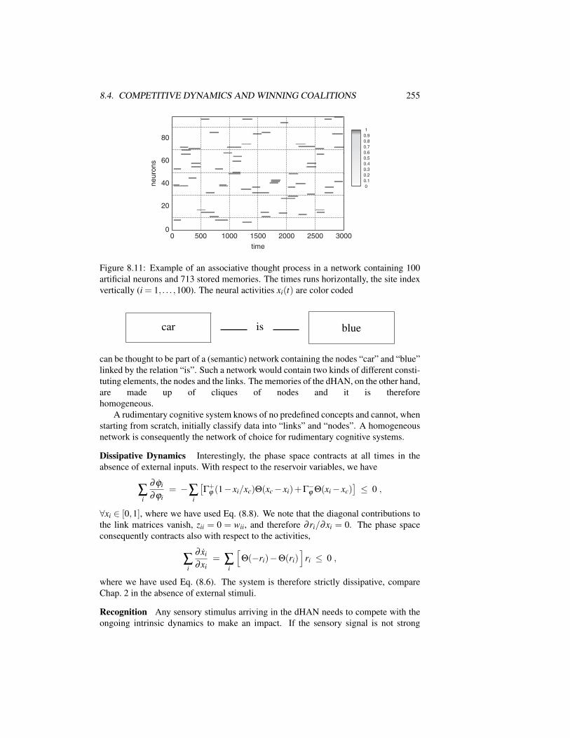
8.4. COMPETITIVE DYNAMICS AND WINNING COALITIONS 255
0
0.1
0.2
0.3
0.4
0.5
0.6
0.7
0.8
0.9
1
time
neuro
ns
0 500 1000 1500 2000 2500 30000
20
40
60
80
Figure 8.11: Example of an associative thought process in a network containing 100artificial neurons and 713 stored memories. The times runs horizontally, the site indexvertically (i = 1, . . . ,100). The neural activities xi(t) are color coded
car is blue
can be thought to be part of a (semantic) network containing the nodes “car” and “blue”linked by the relation “is”. Such a network would contain two kinds of different consti-tuting elements, the nodes and the links. The memories of the dHAN, on the other hand,are made up of cliques of nodes and it is thereforehomogeneous.
A rudimentary cognitive system knows of no predefined concepts and cannot, whenstarting from scratch, initially classify data into “links” and “nodes”. A homogeneousnetwork is consequently the network of choice for rudimentary cognitive systems.
Dissipative Dynamics Interestingly, the phase space contracts at all times in theabsence of external inputs. With respect to the reservoir variables, we have
∑i
∂ ϕi
∂ϕi= −∑
i
[Γ+ϕ (1− xi/xc)Θ(xc− xi)+Γ
−ϕ Θ(xi− xc)
]≤ 0 ,
∀xi ∈ [0,1], where we have used Eq. (8.8). We note that the diagonal contributions tothe link matrices vanish, zii = 0 = wii, and therefore ∂ ri/∂xi = 0. The phase spaceconsequently contracts also with respect to the activities,
∑i
∂ xi
∂xi= ∑
i
[Θ(−ri)−Θ(ri)
]ri ≤ 0 ,
where we have used Eq. (8.6). The system is therefore strictly dissipative, compareChap. 2 in the absence of external stimuli.
Recognition Any sensory stimulus arriving in the dHAN needs to compete with theongoing intrinsic dynamics to make an impact. If the sensory signal is not strong

256 CHAPTER 8. ELEMENTS OF COGNITIVE SYSTEMS THEORY
enough, it cannot deviate the autonomous thought process. This feature results in anintrinsic recognition property of the dHAN: A background of noise will not influencethe transient state dynamics.
8.4.3 Autonomous Online LearningIt is characteristic to the theory of cognitive systems, as pointed out in the introduc-tion (Sect. 8.1), that the exact equations used to model a phenomena of interest are notof importance. There is a multitude of possible formulations and a range of suitablemodeling approaches may lead to similar overall behavior – the principles are moreimportant than the details of their actual implementation. In the preceding section wehave discussed a formulation of transient state dynamics based on competitive cliqueencoding. Within this framework we will now illustrate the basic functioning of home-ostatic regulation.Local Working Point Optimization Dynamical systems normally retain their func-tionalities only when they keep their dynamical properties within certainregimes. They need to regulate their own working point, as discussed in Sect. 8.2.3,via homeostatic regulation. The working point optimization might be achieved eitherthrough diffusive control signals or via local optimization rules. Here we discuss anexample of a local rule.Synaptic Plasticities The inhibitory and the excitatory synaptic strength have differ-ent functional roles in the dHan formulation of transient state dynamics. The averagestrengths |z| and w of the inhibitory and excitatory links differ substantially,
|z| w ,
compare Fig. 8.7. Homeostatic regulation is a slow process involving incrementalchanges. It is then clear that these gradual changes in the synaptic strengths will af-fect dominantly the excitatory links, as they are much smaller, since small changes oflarge parameters (like the inhibitory links) do not influence substantially, quite in gen-eral, the properties of a dynamical system. We may therefore consider the inhibitorybackground as given and fixed and restrict the effect of homeostatic regulation to theexcitatory wi j.Effective Incoming Synaptic Strength The average magnitude of the growth ratesri, see Eq. (8.7), determines the time scales of the autonomous dynamics and thus theworking point. The ri(t) are, however, quite strongly time dependent. The effectiveincoming synaptic signal
ri = ∑j
[wi, jx j + zi, jx j fz(ϕ j)
],
which is independent of the postsynaptic reservoir, ϕi, is a more convenient control pa-rameter for a local homeostatic regulation, since ri tends to the sum of active incominglinks,
ri → ∑j∈α
wi, j ,

8.4. COMPETITIVE DYNAMICS AND WINNING COALITIONS 257
for a transiently stable clique α = (p1, . . . , pZ).
Optimal Growth Rates The working point of the dHan is optimal when the effectiveincoming signal is, on the average, of comparable magnitude r(opt) for all sites,
ri → r(opt) . (8.10)
r(opt) is an unmutable parameter, compare Fig. 8.3. There is no need to fulfill this ruleexactly for every site i. The dHan network will retain functionality whenever Eq. (8.10)is approached slowly and on the average by suitable synaptic plasticities.
Long-Term Homeostatic Plasticities The working point optimization Eq. (8.10) canbe achieved through a suitable local rule:
wi j(t) = Γ(opt)L ∆ri
[ (wi j−W (min)
L
)Θ(−∆ri)+Θ(∆ri)
](8.11)
·Θ(xi− xc)Θ(x j− xc),
− Γ−L d(wi j)Θ(xi− xc)Θ(xc− x j) , (8.12)
with∆ri = r(opt)− ri .
Some comments:
– Hebbian learning: The learning rule Eq. (8.11) is local and of Hebbian type.Learning occurs only when the presynaptic and the postsynaptic neurons areactive. Weak forgetting, i.e. the decay of rarely used links, Eq. (8.12) is localtoo.
– Synaptic Competition: When the incoming signal is weak/strong, relative to theoptimal value r(opt), the active links are reinforced/weakened, with W (min)
L beingthe minimal value for the wi j. The baseline W (min)
L may be chosen to be slightlynegative, compare Fig. 8.7.
The Hebbian-type learning then takes place in the form of a competition betweenincoming synapses – frequently active incoming links will gain strength, on theaverage, on the expense of rarely used links.
– Asymmetric Decay of Inactive Links: The decay term ∝ Γ−L > 0 in Eq. (8.12)
is taken to be asymmetric, viz when the presynaptic neuron is inactive with thepostsynaptic neuron being active. The strength of the decay is a suitable non-linear function d(wi j) of the synaptic strength wi j. Note that the opposite asym-metric decay, for which wi j is weakened whenever the presynaptic/postsynapticneurons are active/inactive, may potentially lead to the dynamical isolation ofthe currently active clique by suppressing excitatory out-of-clique synapses.
– Suppression of Runaway Synaptic Growth: The link dynamics, Eq. (8.11) sup-presses synaptic runaway growth, a general problem common to adaptive andcontinuously active neural networks. It has been shown that similar rules fordiscrete neural networks optimize the overall storage capacity.

258 CHAPTER 8. ELEMENTS OF COGNITIVE SYSTEMS THEORY
– Long-Term Dynamical Stability: In Fig. 8.11 an example for an associativethought process is shown for a 100-site network containing 713 memories. Whenrunning the simulation for very long times one finds that the values of excitatorylinks wi j tend to a steady-state distribution, as the result of the continuous onlinelearning. The system is self-adapting.
Conclusions In this section we presented and discussed the concrete implementationof a module for competitive transient state dynamics within the dHan (dense and ho-mogeneous associative network) approach. Here we have discussed only the isolatedmodule, one can couple this module to a sensory input stream and the competitive neu-ral dynamics will then lead to semantic learning. The winning coalitions of the dHanmodule, the cliques, will then acquire a semantic context, corresponding via their re-spective receptive fields to prominent and independent patterns and objects present inthe sensory stimuli.
The key point is however that this implementation fulfills all requirements neces-sary for an autonomous cognitive system, such as locality of information processing,unsupervised online learning, huge storage capacity, intrinsic generalization capac-ity and self-sustained transient state dynamics in terms of self-generated associativethought processes.
8.5 Environmental Model BuildingThe representation of environmental data, as discussed in Sect. 8.4, allows for simpleassociational reasoning. For anything more sophisticated, the cognitive system needsto learn about the structure of the environment itself, i.e. it has to build models of theenvironment.
The key question is then: Are there universal principles that allow for environmen-tal model building without any a priori information about the environment? Principlesthat work independently of whether the cognitive system lives near a lakeside in atropical rain forest or in an artificial cybernetical world.
Here we will discuss how universal prediction tasks allow for such universal envi-ronmental model building and for the spontaneous generation of abstract concepts.
8.5.1 The Elman Simple Recurrent Network
Innate Grammar Is the human brain completely empty at birth and can babies learnwith the same ease any language, natural or artificial, with arbitrary grammatical orga-nization? Or do we have certain gene determined predispositions toward certain innategrammatical structures? This issue has been discussed by linguists for decades.
In this context in 1990 Elman performed a seminal case study, examining the rep-resentation of time-dependent tasks by a simple recurrent network. This network isuniversal in the sense that no information about the content or structure of the inputdata stream is used in its layout.
Elman discovered that lexical classes are spontaneously generated when the net-work is given the task to predict the next word in an incoming data stream made up ofnatural sentences constructed from a reduced vocabulary.
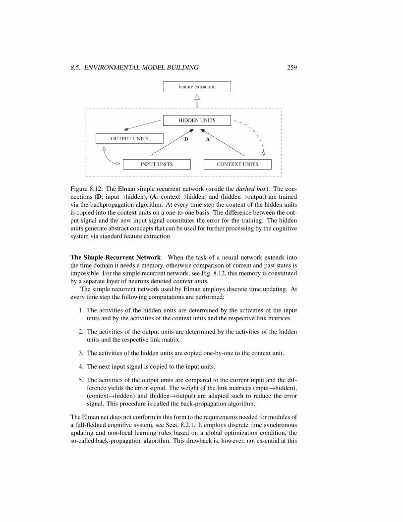
8.5. ENVIRONMENTAL MODEL BUILDING 259
CONTEXT UNITS
HIDDEN UNITS
INPUT UNITS
OUTPUT UNITS
feature extraction
D A
Figure 8.12: The Elman simple recurrent network (inside the dashed box). The con-nections (D: input→hidden), (A: context→hidden) and (hidden→output) are trainedvia the backpropagation algorithm. At every time step the content of the hidden unitsis copied into the context units on a one-to-one basis. The difference between the out-put signal and the new input signal constitutes the error for the training. The hiddenunits generate abstract concepts that can be used for further processing by the cognitivesystem via standard feature extraction
The Simple Recurrent Network When the task of a neural network extends intothe time domain it needs a memory, otherwise comparison of current and past states isimpossible. For the simple recurrent network, see Fig. 8.12, this memory is constitutedby a separate layer of neurons denoted context units.
The simple recurrent network used by Elman employs discrete time updating. Atevery time step the following computations are performed:
1. The activities of the hidden units are determined by the activities of the inputunits and by the activities of the context units and the respective link matrices.
2. The activities of the output units are determined by the activities of the hiddenunits and the respective link matrix.
3. The activities of the hidden units are copied one-by-one to the context unit.
4. The next input signal is copied to the input units.
5. The activities of the output units are compared to the current input and the dif-ference yields the error signal. The weight of the link matrices (input→hidden),(context→hidden) and (hidden→output) are adapted such to reduce the errorsignal. This procedure is called the back-propagation algorithm.
The Elman net does not conform in this form to the requirements needed for modules ofa full-fledged cognitive system, see Sect. 8.2.1. It employs discrete time synchronousupdating and non-local learning rules based on a global optimization condition, theso-called back-propagation algorithm. This drawback is, however, not essential at this
260 CHAPTER 8. ELEMENTS OF COGNITIVE SYSTEMS THEORY
point, since we are interested here in the overall and generic properties of the simplerecurrent network.The Lexical Prediction Task The simple recurrent network works on a time seriesx(t) of inputs
x(1), x(2), x(3), . . .
which are presented to the network one after the other.The network has the task to predict the next input. For the case studied by Elman
the inputs x(t) represented randomly encoded words out of a reduced vocabulary of 29lexical items. The series of inputs corresponded to natural language sentences obeyingEnglish grammar rules. The network then had the task to predict the next word in asentence.The Impossible Lexical Prediction Task The task to predict the next word of anatural language sentence is impossible to fulfill. Language is non-deterministic, com-munication would otherwise convene no information.
The grammatical structure of human languages places constraints on the possiblesequence of words, a verb is more likely to follow a noun than another verb, to give anexample. The expected frequency of possible successors, implicit in the set of trainingsentences, is, however, deterministic and is reproduced well by the simple recurrentnetwork.Spontaneous Generation of Lexical Types Let us recapitulate the situation:
i. The lexical prediction task given to the network is impossible to fulfill.
ii. The data input stream has a hidden grammatical structure.
iii. The frequency of successors is not random.
As a consequence, the network generates in its hidden layer representations of the 29used lexical items, see Fig. 8.13. These representations, and this is the central resultof Elman’s 1990 study, have a characteristic hierarchical structure. Representations ofdifferent nouns, e.g. “mouse” and “cat”, are more alike than the representations of anoun and a verb, e.g. “mouse” and “sleep”. The network has generated spontaneouslyabstract lexical types like verb, nouns of animated objects and nouns of inanimateobjects.Tokens and Types The network actually generated representations of the lexical itemsdependent on the context, the tokens. There is not a unique representation of the itemboy, but several, viz boy1, boy2, . . ., which are very similar to each other, but with finevariations in their respective activation patterns. These depend on the context, as in thefollowing training sentences:
man smell BOY, man chase BOY, ...
The simple recurrent network is thus able to generate both abstract lexical typesand concrete lexical tokens.
Temporal XOR The XOR problem, see Fig. 8.14, is a standard prediction task inneural network theory. In its temporal version the two binary inputs are presented one

8.5. ENVIRONMENTAL MODEL BUILDING 261
smell
move
thinkseeexist
sleepbreak
smash
like
chase
eat
mouse
cat
monster
liondragon
womangirl
man
boy
car
bookrock
sandwichcookie
bread
plate
glass
VERBS
NOUNS
ANIMATES
INANIMATES
humans
animals
food
breakables
transitive (sometimes)
intransitive (always)
transitive (always)
dog
Figure 8.13: Hierarchical cluster diagram of the hidden units activation pattern. Shownare the relations and similarities of the hidden unit activity patterns according to ahierarchical cluster analysis (from Elman, 2004)
after the other to the same input neuron as x(t−1) and x(t), with the task to predict thecorrect x(t +1).
The XOR problem is not linearly decomposable, i.e. there are no constants a,b,csuch that
x(t +1) = ax(t) + bx(t−1) + c ,
and this is why the XOR problem serves as a benchmark for neural prediction tasks.Input sequences like
. . . 000︸︷︷︸ 101︸︷︷︸ 110︸︷︷︸ . . .are presented to the network with the caveat that the network does not know when anXOR-triple starts. A typical result is shown in Fig. 8.14. Two out of three predictionresults are random, as expected but every third prediction is quite good.The Time Horizon Temporal prediction tasks may vary in complexity depending onthe time scale τ characterizing the duration of the temporal dependencies in the inputdata x(t). A well known example is the Markov process.
The Markov Assumption. The distribution of possible x(t) dependsonly on the value of the input at the previous time step, x(t−1).

262 CHAPTER 8. ELEMENTS OF COGNITIVE SYSTEMS THEORY
timestep
0 1 2 3 4 5 6 7 8 9 10 11 12 13
0.1
0.15
0.2
0.25
squ
are
d e
rror
x(t-1) x(t) x(t+1)
0
1
1
0
0
1
0
1
0
0
1
1
Figure 8.14: The temporal XOR. Left: The prediction task. Right: The performance(y(t+1)−x(t+1))2 (y(t)∈ [0,1] is the activity of the single output neuron of a simplerecurrent network, see Fig. 8.12, with two neurons in the hidden layer after 600 sweepsthrough a 3000-bit training sequence
For Markovian-type inputs the time correlation length of the input data is 1; τ = 1.For the temporal XOR problem τ = 2. In principle, the simple recurrent network isable to handle time correlations of arbitrary length. It has been tested with respectto the temporal XOR and to a letter-in-a-word prediction task. The performance ofthe network in terms of the accuracy of the prediction results, however, is expected todeteriorate with increasing τ .
8.5.2 Universal Prediction Tasks
Time Series Analysis The Elman simple recurrent network is an example of a neuralnetwork layout that is suitable for time series analysis. Given a series of vectors
x(t), t = 0, 1, 2, . . .
one might be interested in forecasting x(t + 1) when x(t), x(t − 1), . . . are known.Time series analysis is very important for a wide range of applications and a plethoraof specialized algorithms have been developed. State Space Models Time series
generated from physical processes can be described by “state space models”. Thedaily temperature in Frankfurt is a complex function of the weather dynamics, whichcontains a huge state space of (mostly) unobservable variables. The task to predictthe local temperature from only the knowledge of the history of previous temperaturereadings constitutes a time series analysis task.
Quite generally, there are certain deterministic or stochastic processes generating aseries
s(t), t = 0, 1, 2, . . .
of vectors in a state space, which is mostly unobservable. The readings x(t) are thensome linear or non-linear functions
x(t) = F[s(t)] + η(t) (8.13)

8.5. ENVIRONMENTAL MODEL BUILDING 263
of the underlying state space, possibly in addition to some noise η(t). Equation (8.13)is denoted a state space model.
The Hidden Markov Process There are many possible assumptions for the statespace dynamics underlying a given history of observables x(t). For a hidden Markovprocess, to give an example, one assumes that
(a) s(t + 1) depends only on s(t) (and not on any previous state space vector, theMarkov assumption) and that
(b) the mapping s(t)→ s(t +1) is stochastic.
The process is dubbed “hidden”, because the state space dynamics is not directly ob-servable.
The Elman State Space Model The dynamics of the Elman simple recurrent networkis given by
s(t) = σ[As(t−1)+Dx(t)
], σ [y] =
11+ e−y , (8.14)
were x(t) and s(t) correspond to the activation patterns of input and hidden units, re-spectively. The A and D are the link matrices (context→hidden) and (input→hidden),compare Fig. 8.12, and σ(y) is called the sigmoid function. The link matrix (hidden→output) corresponds to the prediction task s(t)→ x(t + 1) given to the Elman net-work.
The Elman simple recurrent network extends the classical state space model. Fora normal state space model the readings x(t) depend only on the current state s(t) ofthe underlying dynamical system, compare Eq. (8.13). Extracting x(t) from Eq. (8.14),one obtains
x(t) = F[s(t),s(t−1)] , (8.15)
which is a straightforward generalization of Eq. (8.13). The simple recurrent net has amemory since x(t) in Eq. (8.15) depends both on s(t) and on s(t−1).
Neural Networks for Time Series Analysis The simple recurrent network can begeneralized in several ways, e.g. additional hidden layers result in a non-linear statespace dynamics. More complex layouts lead to more powerful prediction capabilities,but there is a trade-off. Complex neural networks with lots of hidden layers and recur-rent connections need very big training data. There is also the danger of overfitting thedata, when the model has more free parameters than theinput.
Time Series Analysis for Cognitive Systems For most technical applications oneis interested exclusively in the time prediction capability of the algorithm employedand an eventual spontaneous generation of abstract concepts is not of interest. Puretime series prediction is, however, of limited use for a cognitive system. An algorithmallowing the prediction of future events that at the same time generates models of theenvironment is, however, extremely useful for a cognitive system.

264 CHAPTER 8. ELEMENTS OF COGNITIVE SYSTEMS THEORY
This is the case for state space models, as they generate explicit proposals for theunderlying environmental states describing the input data. For the simple recurrentnetwork these proposals are generated in the hidden units. The activation state ofthe hidden units can be used by the network for further cognitive information pro-cessing via a simple feature extraction procedure, see Fig. 8.12, e.g. by a Kohonenlayer.14
Possible and Impossible Prediction Tasks A cognitive system is generally con-fronted with two distinct types of prediction tasks.
– Possible Prediction Tasks: Examples are the prediction of the limb dynamics asa function of muscle activation or the prediction of physical processes like themotion of a ball in a soccer game.
– Impossible Prediction Tasks: When a series of events is unpredictable it is, how-ever, important to be able to predict the class of the next events. When we drivewith a car behind another vehicle we automatically generate in our mind a set oflikely maneuvers that we we expect the vehicle in front of us to perform next.When we listen to a person speaking we generate expectancies of what the per-son is likely to utter next.
Universal Prediction Tasks and Abstract Concepts Impossible prediction tasks,like the lexical prediction task discussed in Sect. 8.5.1, lead to the generation of ab-stract concepts in the hidden layer, like the notion of “noun” and “verb”. This is nota coincidence, but a necessary consequence of the task given to the network. Onlyclasses of future events can be predicted in an impossible prediction task and not con-crete instances. We may then formulate the key result of this section in the form of alemma.
Universal Prediction Task Lemma. The task to predict future eventsleads to universal environmental model building for neural networks withstate space layouts. When the prediction task is impossible to carry out,the network will automatically generate abstract concepts that can be usedfor further processing by the cognitive system.
Conclusions Only a small number of genes, typically a few thousands, are responsiblefor the growth and the functioning of mammalian brains. This number is by far smallerthan the information content which would be required for an explicity encoding of themyriad of cognitive capabilities of mammalian brains. All these cognitive skills, apartfrom a few biologically central tasks, must result from a limited number of universalprinciples, the impossible time prediction task being one of them.
14A Kohonen network is an example of a neural classifier via one-winner-takes-all architecture, see e.g.Ballard (2000).

Further Reading 265
Exercises
TRANSIENT STATE DYNAMICSConsider a system containing two variables, x,ϕ ∈ [0,1]. Invent a system ofcoupled differential equations for which x(t) has two transient states, x ≈ 1 andx ≈ 0. One possibility is to consider ϕ as a reservoir and to let x(t) autoex-cite/autodeplete itself when the reservoir is high/low.
The transient state dynamics should be rigorous. Write a code implementing thedifferential equations.
THE DIFFUSIVE CONTROL UNITGiven are two signals y1(t) ∈ [0,∞] and y2(t) ∈ [0,∞]. Invent a system of differ-ential equations for variables x1(t) ∈ [0,1] and x2(t) ∈ [0,1] driven by the y1,2(t)such that x1→ 1 and x2→ 0 when y1 > y2 and vice versa. Note that the y1,2 arenot necessarily normalized.
LEAKY INTEGRATOR NEURONSConsider a two-site network of neurons, having membrane potentials xi and
activities yi ∈ [−1,1], the so-called “leaky integrator” model for neurons,
x1 = −Γx1−wy2, x2 = −Γx2 +wy1, yi =2
e−xi +1−1 ,
with Γ > 0 being the decay rate. The coupling w > 0 links neuron one (two)excitatorily (inhibitorily) to neuron two (one). Which are the fixpoints and forwhich parameters can one observe weakly damped oscillations?
ASSOCIATIVE OVERLAPS AND THOUGHT PROCESSESConsider the seven-site network of Fig. 8.6. Evaluate all pairwise associativeoverlaps of order zero and of order one between the five cliques, using Eqs. (8.4)and (8.5). Generate an associative thought process of cliques α1, α2, . . ., wherea new clique αt+1 is selected using the following simplified dynamics:
(1) αt+1 has an associative overlap of order zero with αt and is distinct fromαt−1.
(2) If more than one clique satisfies criterium (1), then the clique with the high-est associative overlap of order zero with αt is selected.
(3) If more than one clique satisfies criteria (1)–(2), then one of them is drawnrandomly.
Discuss the relation to the dHAN model treated in Sect.8.4.2.
Further ReadingFor a general introduction to the field of artificial intelligence (AI), see Russell andNorvig (1995). For a handbook on experimental and theoretical neuroscience, see

266 8 Elements of Cognitive Systems Theory
Arbib (2002). For exemplary textbooks on neuroscience, see Dayan and Abbott (2001)and for an introduction to neural networks, see Ballard (2000).
Somewhat more specialized books for further reading regarding the modeling ofcognitive processes by small neural networks is that by McLeod et al. (1998) and oncomputational neuroscience that by O’Reilly and Munakata (2000).
For some relevant review articles on dynamical modeling in neuroscience the fol-lowing are recommended: Rabinovich et al. (2006); on reinforcement learning Kael-bling et al. (1996), and on learning and memory storage in neural nets Carpenter(2001).
We also recommend to the interested reader to go back to some selected original lit-erature dealing with “simple recurrent networks” in the context of grammar acquisition(Elman, 1990; 2004), with neural networks for time series prediction tasks (Dorffner,1996), with “learning by error” (Chialvo and Bak, 1999), with the assignment of thecognitive tasks discussed in Sect. 8.3.1 to specific mammal brain areas (Doya, 1999),with the effect on memory storage capacity of various Hebbian-type learning rules(Chechik et al. 2001), with the concept of “associative thought processes” (Gros, 2007;2009a) and with “diffusive emotional control” (Gros, 2009b).
It is very illuminating to take a look at the freely available databases storing humanassociative knowledge (Nelson et al. 1998; Liu and Singh, 2004).
ABELES M. ET AL. 1995 Cortical activity flips among quasi-stationary states. Proceedingsof the National Academy of Science, USA 92, 8616–8620.
ARBIB, M.A. 2002 The Handbook of Brain Theory and Neural Networks. MIT Press, Cam-bridge, MA.
BAARS, B.J., FRANKLIN, S. 2003 How conscious experience and working memory interact.Trends in Cognitive Science 7, 166–172.
BALLARD, D.H. 2000 An Introduction to Natural Computation. MIT Press, Cambridge, MA.
CARPENTER, G.A. 2001 Neural-network models of learning and memory: Leading questionsand an emerging framework. Trends in Cognitive Science 5, 114–118.
CHECHIK, G., MEILIJSON, I., RUPPIN, E. 2001 Effective neuronal learning with ineffectiveHebbian learning rules. Neural Computation 13, 817.
CHIALVO, D.R., BAK, P. 1999 Learning from mistakes. Neuroscience 90, 1137–1148.
CRICK, F.C., KOCH, C. 2003 A framework for consciousness. Nature Neuroscience 6, 119–126.
DAYAN, P., ABBOTT, L.F. 2001 Theoretical Neuroscience: Computational and Mathemati-cal Modeling of Neural Systems. MIT Press, Cambridge, MA.
DEHAENE, S., NACCACHE, L. 2003 Towards a cognitive neuroscience of consciousness: Ba-sic evidence and a workspace framework. Cognition 79, 1–37.
DORFFNER, G. 1996 Neural networks for time series processing. Neural Network World 6,447–468.
DOYA, K. 1999 What are the computations of the cerebellum, the basal ganglia and the cere-bral cortex? Neural Networks 12, 961–974.
EDELMAN, G.M., TONONI, G.A. 2000 A Universe of Consciousness. Basic Books, NewYork.
ELMAN, J.L. 1990 Finding structure in time. Cognitive Science 14, 179–211.

Further Reading 267
ELMAN, J.L. 2004 An alternative view of the mental lexicon. Trends in Cognitive Sciences8, 301–306.
GROS, C. 2007 Neural networks with transient state dynamics. New Journal of Physics 9,109.
GROS, C. 2009a Cognitive computation with autonomously active neural networks: an emerg-ing field. Cognitive Computation 1, 77.
GROS, C. 2009b Emotions, diffusive emotional control and the motivational problem for au-tonomouscognitive systems, in Handbook of Research on Synthetic Emotionsand Socia-ble Robotics: New Applications in Affective Computing and Artificial Intelligence, J. Val-lverdu, D. Casacuberta (Eds). IGI-Global.
KAELBLING, L.P., LITTMAN, M.L., MOORE, A. 1996 Reinforcement learning: A survey.Journal of Artificial Intelligence Research 4, 237–285.
KENET, T., BIBITCHKOV, D., TSODYKS, M., GRINVALD, A., ARIELI, A. 2003 Sponta-neously emerging cortical representations of visual attributes. Nature 425, 954–956.
LIU, H., SINGH, P. 2004 ConcepNet a practical commonsense reasoning tool-kit. BT Tech-nology Journal 22, 211–226.
MCLEOD, P., PLUNKETT, K., ROLLS, E.T. 1998 Introduction to Connectionist Modelling.Oxford University Press New York.
NELSON, D.L., MCEVOY, C.L., SCHREIBER, T.A. 1998 The University of South FloridaWord Association, Rhyme, and Word Fragment Norms. Homepage: http://www.usf.edu/FreeAssociation.
O’REILLY, R.C., MUNAKATA, Y. 2000 Computational Explorations in Cognitive Neuro-science: Understanding the Mind by Simulating the Brain. MIT Press Cambridge.
RABINOVICH, M.I., VARONA, P., SELVERSTON, A.I. AND ABARBANEL, H.D.I. 2006 Dy-namical principles in neuroscience. Review of Modern Physics 78, 1213–1256.
RUSSELL, S.J., P NORVIG, P. 1995 Artificial Intelligence: A Modern Approach. Prentice-Hall, Englewood Cliffs, NJ.

268 8 Elements of Cognitive Systems Theory