adaptive dynamics studying the dynamic change of community dynamical parameters through mutation and...

Adaptive Dynamics

studying the dynamic change of community dynamical parameters

through mutation and selection

Hans (= J A J *) Metz

(formerly ADN) IIASA

QuickTime™ en eenTIFF (ongecomprimeerd)-decompressorzijn vereist om deze afbeelding weer te geven.

VEOLIA-Ecole Poly-technique

QuickTime™ en eenTIFF (ongecomprimeerd)-decompressor

zijn vereist om deze afbeelding weer te geven.

&Mathematical Institute, Leiden University

QuickTime™ and a decompressor

are needed to see this picture.

preamble: some terminology

micro-evolution: changes in gene frequencies on a population dynamical time scale,

meso-evolution: evolutionary changes in the values of traits of representative individuals and concomitant patterns of taxonomic diversification (through multiple mutant substitutions),

macro-evolution: changes where one cannot even speak in terms of a fixed set of traits, like anatomical innovations.

Goal: get a mathematical grip on meso-evolution.

functiontrajectories

formtrajectories

genome

development

selection

(darwinian)

(causal)

demography

physics

almost faithful reproduction

ecology

(causal)

fitness

environment

components of the evolutionary mechanism

fitness

functiontrajectories

formtrajectories

genome

development

selection

(darwinian)

(causal)

physics

almost faithful reproduction

ecology

(causal)environment

Adaptive Dynamics

demography

AD’s basis in Commmunity Dynamics

Populations are considered as measures over a space ot i(ndividual)-states (e.g. spanned by age and size).

Environments (E) are delimited such that given their environment individuals are independent,

and hence their mean numbers have linear dynamics.Resident populations are assumed to be so large that

we can approximate their dynamics deterministically.These resident populations influence the environment

so that they do not grow out of bounds.The resulting dynamical systems therefore have

attractors, which are assumed to produce ergodic environments.


Mutants enter the population singly.Therefore, initially their impact on the environment can

be neglected. The initial growth of a mutant population can be

approximated with a branching process. Invasion fitness is the (generalised) Malthusian parameter

(= averaged long term exponential growth rate of the mean) of this proces: (Existence guaranteed by the multiplicative ergodic theorem.)

Residents have fitness zero.


resident population size

population sizes of

other species

mutantpopulationsize

fitness as dominant transversal eigenvalue

resident population size

population sizes of

other species

mutantpopulationsize

or, more generally, dominant transversal Lyapunov exponent


Fitnesses are not given quantities, but depend on (1) the traits of the individuals, X, Y, (2) the environment in which they live:

(Y | E)The latter is set by the resident community:

E = Eattr(C), C={X1,...,Xk)

biological implications

Evolutionary progress is almost exclusively determined by the fitnesses of potential mutants.

AD: fitness landscapes change with evolution

Evolution proceeds through uphill movements in a fitness landscape that keeps changing so as to keep the fitness of the resident types at exactly zero.

Evolution proceeds through uphill movements in a fitness landscape

resident trait value(s) x

evol

utio

nary

tim

e

0

0

0

fitness landscape: (y,E(t))

mutant trait value y

0

0

type

morph

strategy

trait vector

point (in trait space)

type

morph

strategy

trait vector (trait value)

point (in trait space)

effective synonyms

The different spaces that play a role in adaptive dynamics:

the trait space in which their evolution takes place(= parameter space of their i- and therefore of their p-dynamics)

= the ‘state space’ of their adaptive dynamics

the physical space inhabited by the organisms

the state space of their i(ndividual)-dynamics

the space of the influences that they undergo(fluctuations in light, temperature, food, enemies, conspecifics):

their ‘environment’

the parameter spaces of families of adaptive dynamics

the state space of their p(opulation)-dynamics

scaling up from organisms to trait evolution

the simplifications underlying AD

essential formost conclusions

i.e., separated population dynamical and mutational time scales:the population dynamics relaxes before the next mutant comes

1. mutation limited evolution

2. clonal reproduction

3. good local mixing4. largish system sizes

5. “good” c(ommunity)-attractors6. interior c-attractors unique

7. fitness smooth in traits8. small mutational steps

essential conceptuallly

essential

from CD to AD: nature of the limits

x

adaptive dynamicslimit

individual-basedsimulation

classical largenumber limit

t

, rescale time, only consider traits

rescale numbers to densities

= system size, = mutations / birth

t

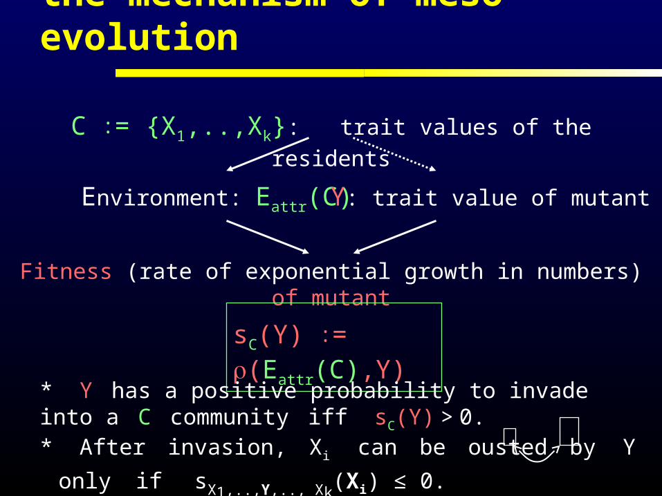
the mechanism of meso-evolution

C := {X1,..,Xk}: trait values of the residents

Environment: Eattr(C) Y: trait value of mutant

Fitness (rate of exponential growth in numbers) of mutant

sC(Y) := (Eattr(C),Y)

* Y has a positive probability to invade into a C community iff sC(Y) > 0.

* After invasion, Xi can be ousted by Y only if sX1,..,Y,.., Xk(Xi) ≤ 0.

* For small mutational steps Y takes over, except near so-called “ess”es.

time1

10

100

1000

10 200

# individuals

population dynamics: branching process results

or "grow exponentially” either go extinct, mutant populations starting from single individuals

In an a priori given ergodic environment:

(with a probability that to first order in | Y – X | is proportional

to their (fitness)+ , and with their fitness as rate parameter).

Invasion of a "good" c-attractor of X leads to a substitution such that this c-attractor is inherited by Y Y and up to O(2),

sY(X) = – sX(Y).

community dynamics: ousting the resident?

Proposition:

Let = | Y – X | be sufficiently small,

and let X not be close to an “evolutionarily singular strategy”, or to a c(ommunity)-dynamical bifurcation point.

“For small mutational steps invasion implies substitution.”

community dynamics: sketch of the proof

When an equilibrium point or a limit cycle is invaded, the relative frequency p of Y satisfies

= sX(Y) p(1-p) + O(2),

while the convergence of the dynamics of the total population densities occurs O(1).

dpdt

1

03 4 5 6 7

p

sX(Y) t

Singular strategies X* are defined by sX*(Y) = O(), instead of O().

Near where the mutant trait value y equals the resident trait value x there is a degenerate transcritical bifurcation:

community dynamics: the bifurcation structure

nx →

↑ny

n x→

↑ny

n x →

↑ny

y<xy=xy>x

community dynamics: the bifurcation structure

relativefrequency

of 2nd

'species'resident trait value x

0

1


resident trait value x0

1


evolution will be towards increasing x

evolution will be towards decreasing x

Near where the mutant trait value y equals the resident trait value x there is a degenerate transcritical bifurcation:

The effective speeds of evolutionary change are proportional to the probabilities that invading mutants survive the initial stochastic phase

population dynamics: the bifurcation structure

probability thatmutant

invades

evolution will be towards increasing x

evolution will be towards decreasing x

Near where the mutant equals the resident, the probability that the mutant invades changes as depicted below:

The effective speeds of evolutionary change are proportional to the probabilities that invading mutants survive the initial stochastic phase


1



1


+

+

-

y

x

-

fitness contour plotx: residenty: potential mutant

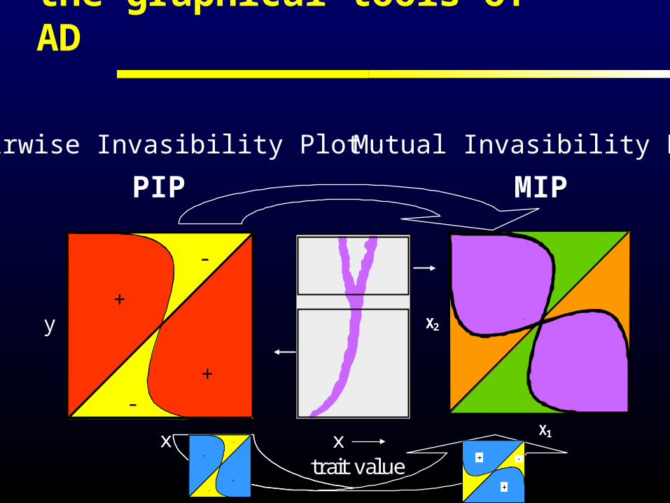
the graphical tools of AD

trait valuex

x0x1

x1

x2

x

X

X1

2

+

-

+

-

.

Mutual Invasibility Plot

MIP

y

xtrait value

X

x


+

+

-

-

Pairwise Invasibility Plot

PIP

y

x0

+

+

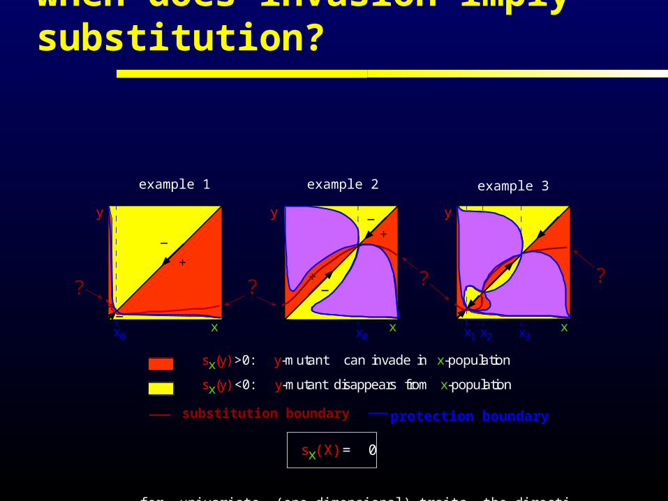
example 1 example 2

+

+

x0

sx(y) >0: y-mutant can invade in x-population

sx(y) <0: y-mutant disappears from x-population

for univariate (one-dimensional) traits the direction of evolution is determined by sign sx(y)

sx(X) = 0

example 3

x x1 x2 x3

y y

x x

when does invasion imply substitution?

? ? ? ?

substitution boundary protection boundary

X2

X1

trait valuex

Trait Evolution Plot

TEP

x2


y

x

+

+

-

-

Pairwise Invasibility Plot

PIP

evolutionarily singular strategies

x*

x0

+

+

x*

x* is a singular point iff

dy

dsx(y) = 0y=x=x*

(x* is an extremum in the y-direction)

x*

x*

+

+

y

x* x

v=y-x*

u=x-x*

su(v) = a + b1u+b0v + c11u2+2c10uv+c00v2

+ h.o.t

b1=b0=0

a=0b1+b0=0c11+2c10+c00=0

neutrality of resident

x* is an extremum in y

s0(0)=0

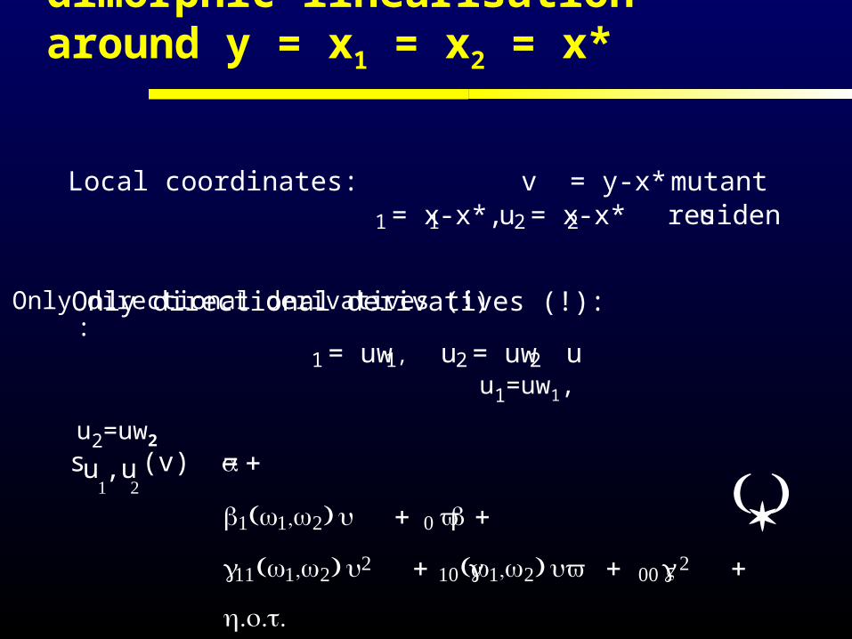
su(u)=0su(v) = c11u2−(c11+c) +uv cv

+ . .h o t

(monomorphic) linearisation around y = x = x*

c11+2c10+c00=0

a=0b1+b0=0

neutrality of resident

su(u)= 0

b1=b0=0

x* is an extremum in y

s0(0)=0

su(v) = c11u2−(c11+c) +uv cv

+ . .h o t

monomorphicconvergenceto x0

yes

no

c00

noyes

noyes

c11c11

c00

x0 uninvadable

local PIP classification

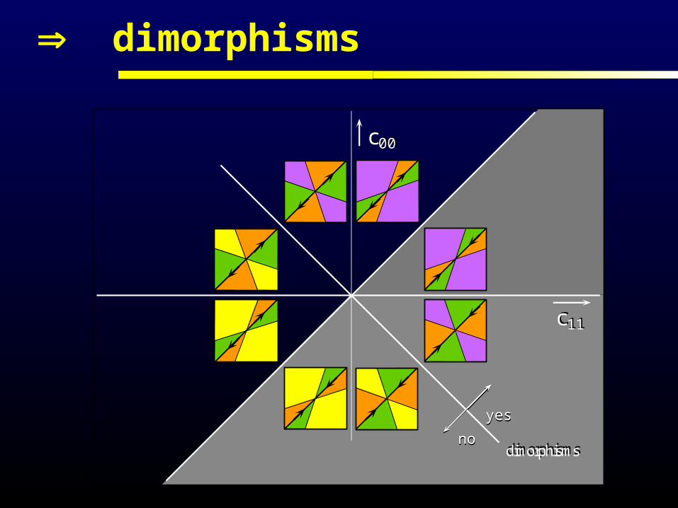
dimorphisms

c00

c11c11

c00

dimorphismsnono

yesyes

dimorphisms

dimorphic linearisation around y = x1 = x2 = x*

Local coordinates: v = y-x* mutant u1 = x1-x*, u2 = x2-x*

residents

Only directional derivatives (!):

u1 = uw1, u2 = uw2

Only directional derivatives (!)

n1 →

n1→^

↑

n2^

↑n2

A

B

B

A

community state space parameter space

parameter paths attractor paths

A

B

A

B

population dynamics: non-genericity strikes


su ,u (v) = α+

β1(w1,w)u+β v +

γ11(w1,w)u+γ1(w1,w)uv+γV+

. . .h o t

1 (*)

Local coordinates: v = y-x* mutant u1 = x1-x*, u2 = x2-x*

residents

Only directional derivatives (!):

u1 = uw1, u2 = uw2

Only directional derivatives (!) :

u1=uw1, u2=uw2


s00 (v) = s0(v)

su ,u (u1) = 0 =1 2

su ,u (u2)1 2

neutrality of residents

su ,u (v) =1 2

su ,u (v)2 1

symmetry

if u1=u2=0 we are back in themonomorphic resident case

su ,u (v) =1 2

expansion formula (*)

(v-u1) (v-u2) [c00+ h.o.t]

local types of dimorphic evolution

0

c00>0

V0

u1 u2

Su ,u (v)1 2

Su ,u (v) = (v-u1) (v-u2) [c00+ h.o.t]1 2

c00<0

Su ,u (v)1 2

V

u1 u2

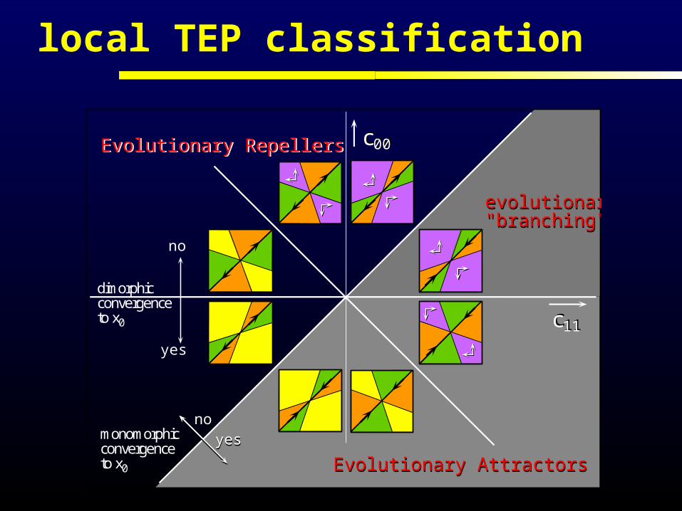
local TEP classification

monomorphicconvergenceto x0

dimorphicconvergenceto x0

yes

no

evolutionary"branching"evolutionary"branching"

Evolutionary AttractorsEvolutionary Attractors

Evolutionary RepellersEvolutionary Repellers c00

noyes

noyes

c11c11

c00

more about adaptive branching

t r a i t v a lu e

x

evol

utio

nary

tim

e

t i m e t r a

i t

fitne

ssfitness

minimum

population

. Summary

Ecological Character Simulation

beyond clonality: thwarting the Mendelian mixer

asso

rtativ

enes

s

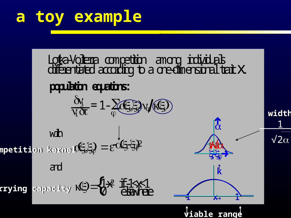
a toy example

____ = 1 - Σa(xi,xj)nj/k(xi)dninidt j

k(x)=

a(xi,xj)=e-α(xi-xj) xi-xj→xi-xj→

↑a↑a

1/√α1/√α

Lotka-Volterra competition among individualsdifferentiated according to a one-dimensional trait x.

with

and

population equations:

1-x2 if -1<x<10 elsewhere{

↑k

-1 x → 1

↑k

-1 x → 1

Lotka-Volterra all per capita growth rates are linear functions of the population densities

Lotka-Volterra all per capita growth rates are linear functions of the population densities

LV models are unrealistic, but useful since they have explicit expressions for the invasion fitnesses.

a toy example

____ = 1 - Σa(xi,xj)nj/k(xi)dninidt j

k(x)=

a(xi,xj)=e-α(xi-xj) xi-xj→xi-xj→

↑a↑a

1/√α1/√α

Lotka-Volterra competition among individualsdifferentiated according to a one-dimensional trait x.

with

and

population equations:

1-x2 if -1<x<10 elsewhere{

↑k

-1 x → 1

↑k

-1 x → 1

viable range

competition kernelcompetition kernel

carrying capacity carrying capacity

widthwidth 1 ––––––––

√2α

matryoshka galore

x1

x

x2

Exploring parameter space

α=1/3: α=: α=3:

isoclines correspond to loci of monomorphic singular points.

interrupted: branching prone ( trimorphically repelling)

x1

x

x2

Exploring parameter space

α=1/3: α=: α=3:

of two lines about to merge one goes extinct

matryoshka galore polymorphisms are invariant under permutation of indices

X2

the six purple

volumesshould

be identified

!

adjacent purple volumes are mirror symmetric around a diagonal plane

X1

X3

matryoshka galore the sets of trimorphisms connect to the isoclines of the dimorphisms

isoclineof

species 1

isoclineof

species 3

X1

X2

X3

(x2 = x3) (x2 = x1)

more consistency conditions!

There also exist various global consistency relations!

The classification of the singular points was based on just a smoothness assumption and some ecologically reasonable consistency conditions.

x2

x1

y

x

+

-

+

-

is extinct. the coexistence set one type. Use that on the boundaries of

a more complicated example

.

Seed size 2

Seed size 1

seed size evolution: TEPs

a potential difficulty: heteroclinic loops

1 2

3

1 2

3

1 2

3

1 2

3

1 2 1 2

3 3

?

a potential difficulty: heteroclinic loops

4

3

1

2

4

23

1

?

The larger the number of types, the larger the fraction ofheteroclinic loops among the possible attractor structures !

much remains to be done!

(Many partial results are floating around.)

Classify the geometries of the fitness landscapes, and coexistence sets near singular points in higher dimensions.

Develop a fullfledged bifurcation theory for AD.

Develop (more) global geometrical results. Delineate to what extent, and in which manner, AD results stay intact

for Mendelian populations.Develop analogous theories for not fully smooth s-

functions.

Analyse how to deal with the heteroclinic loop problem.

(Some recent results by Odo and Barbara Boldin.)

The end

adaptive dynamics studying the dynamic change of community dynamical parameters through mutation and...

Documents