comparison of land water storage from global hydrologic and … · 2018-09-07 · comparison of...

Comparison of Land Water Storage from Global Hydrologic and Land Surface Models and GRACE

Satellites

Bridget R. Scanlon

1Bureau of Economic Geology, Jackson School of Geosciences, Univ. of Texas at Austin, Austin, Texas, United States

Collaborators

Zizhan Zhang, Institute of Geodesy and Geophysics, Wuhan, China

Ashraf Rateb, Bur. Econ. Geol., Jackson School of Geosci., Univ. of Texas at Austin

Himanshu Save, Center for Space Research, Univ. of Texas at Austin

David N. Wiese, NASA Jet Propulsion Lab., Pasadena, California

Michael Croteau, Univ. of Colorado, Boulder, Colorado

David Lawrence, Univ. Corporation for Atmospheric Research, Boulder, Colorado

Zong Liang Yang, Dept. Geol. Sciences, Jackson School of Geosciences, Univ. of Texas at Austin

Hiroko Beaudong, Goddard Space Flight Center, Univ. of Maryland

Hannes Müller Schmied, Goethe University, Frankfurt, Germany

Rens van Beek, Utrecht University, Utrecht

Robert C. Reedy, Bur. Econ. Geol., Jackson School of Geosci., Univ. of Texas at Austin

Alex Sun, Bur. Econ. Geol., Jackson School of Geosci., Univ. of Texas at Austin

Outline

• Background1. GRACE satellites2. Global models

• Objectives

• Results1. Comparison of modeled water storage with GRACE

signals2. Evaluation of human intervention on water storage3. Impact of land water storage on global mean sea level

GRACEGravity Recovery and Climate Experiment

2002 - 2017GRACE Follow-On: May 2018

Satellites: 450 km above land surface220 km apart

Spatial resolution ~ 100,000 km2

~ 90 mins for circum-polar orbit

Monthly data1 gigaton mass change = 1 km3 of water

Only satellite to penetrate deep into subsurface

Total water storage changeSnow, surface water, soil moisture, and groundwater

http://grace.jpl.nasa.gov/mission/gravity-101/


How GRACE Works

GPS Ground Receiver

Mass Anomaly

GPS Satellites

Nominal Separation

GRACE: giant weighing scale in the skyGRACE satellites measure time variable gravityfield

GRACE satellitesare the instruments

How GRACE Works

GPS Ground Receiver

Mass Anomaly

GPS Satellites

Leading satellite approaches the anomaly andfeels a greater gravitational attraction:

Separation Velocity Increases

How GRACE Works

GPS Ground Receiver

Mass Anomaly

GPS Satellites

Trailing satellite approaches the anomaly andcatches up:

Separation Velocity Decreases

How GRACE Works

GPS Ground Receiver

Mass Anomaly

GPS Satellites

Leading satellite is no longer affected by the anomaly whilethe trailing satellite is being pulled backwards:

Separation Velocity Increases

How GRACE Works

GPS Ground Receiver

Mass Anomaly

GPS Satellites

Trailing satellite catches back up to the leading satelliteThe mass anomaly has been observed in the KBR data

How GRACE Works

• By measuring the distance between the two satellites, GRACE estimates changes in gravity

• Dominant control on temporal variations in gravity at monthly scales is water distribution

• GRACE estimates changes in Total Water Storage from the atmosphere to the Moho

• GRACE resolution is low and can only be applied to large scale basins (> ~100,000 km2)

• We can convert gravity change to equivalent water height or volume at Earth’s surface

• 1 gigaton mass change = 1 km3 of water

Global Models

Groundwater depletion (Wada et al., 2010)

Reservoir storage: decrease rate of sea level riseGW depletion, increase rate of sea level rise

We need models to make projections:• Impacts of climate change and human

intervention on water resources

UNESCO World Water Assessment ProgramGlobal assessments of water resources Wada et al., 2016

IPCC, impact of land water storage on sea level rise

SnWS, Snow water storageSWS: Surface water storage

SMS: soil moisture storage

GWS: groundwater storage

RESS

soil moisture

groundwater

SnWS

Global ModelsInput – Output = Change in Storage

Precip. – ET – Roff – Ext. = DTWSExt. human water extraction

GRACE (Change in Total Water Storage, DTWS)

SnWS from SNODAS or Global or National Land Data Assimilation System (GLDAS or NLDAS) land surface models (LSMs)SWS: reservoir storage monitored in some regions, altimetrySMS: estimated from land surface models (GLDAS or NLDAS)GLDAS: Land surface models: NOAH, MOSAIC, VIC, CLM, CLSMNLDAS: NOAH, MOSAIC, and VIC LSMs

RESS

soil moisture

groundwater

SnWS SnWS, Snow water storageSWS: Surface water storage

SMS: soil moisture storage

GWS: groundwater storage

Global Models

1. Global hydrologic models• Developed to assess water scarcity

– daily, water balance, – snow, surface water, soil moisture and groundwater, – human water use and reservoir management

2. Land Surface Models (LSMs)

– Lower boundary condition for global climate models– More physically based, including energy budget – Snow and soil moisture – No human water use or reservoir management

Model Attributes

MO

DEL

WG

HM

PC

R-

GLO

BW

B

VIC

NO

AH

-3.3

CLS

M-F

2.5

CLM

-4.0

Parameter GHWRMs Land Surface Models

Precip. WFDEI CMAP PGMFD CRU-NCEP

SWS x x x

SMS

GWS x x

Hum. Int. x x x x

SW rout. x x x

Soil lay. (no.)1 2 3 4 10 10

Soil (m) 2.0* 1.5 3.5 3.5 3.4 3.4

GHWRM: Global Hydrologic and Water Resource Models

Only WGHM is calibrated

Objectives

1. What is the relative contribution of different signals to the total signal?

2. How do modeled storage changes compare with those from GRACE?

3. What is the impact of human intervention on water storage?

4. What is the impact of land water storage trends on global mean sea level?

5. What is causing the differences between models and GRACE?

Objectives and Responses 1. What is the relative contribution of different signals to the total signal?

Seasonal signals dominant, 51 – 75% of total signal, trends ≤ 5% of total signal.


Models underestimate trends.


Human intervention reduces global water storage (56 – 86 km3/yr) but does not impact seasonal amplitudes at the basin scale.

4. What is the impact of land water storage trends on global mean sea level (GMSL)?

GRACE data indicate net increase in land water storage globally (71 – 82 km3/yr) which contributes negatively to GMSL whereas models indicate decreases in water storage (-450 to -12 km3/yr).


Lack of storage compartments and limited capacity

Uncertainties in fluxes

ModelsGHMs

GRACE

SphericalHarmonics

MasconsGHWRMs LSMs

WGHM PCR-GLOBWB

NOAH

MOSAIC

VIC

CLM

± Human water use

Total Water StorageAnomalies

CSR-GSHCSR-GSH.sf

CSR-MJPL-M.dsf

Time series decomposition

• Long-term trends• Seasonal• Interannual• Residual

ControlsBasin size, climate, irrigation

Total Water Storage

Anomalies

P – ET ± Q –EX – D = ΔTWS GRACECanopySWSSMS

SWS SWSSMSGWS

CanopySnowSWSSMSGWS

Total Water Storage Anomalies, 186 river basins, ~ 60% of land surface

Amazon

Ganges

Euphrates

Murray

Hai

Okavango

Arkansas

Scanlon et al., PNAS, 2018

1. What is the relative contribution of different signals to the total signal?Example: GRACE CSR-Mascons

Stotal = Slong-term + Sinterannual + Sseasonal + residuals

0

20

40

60

80

100

1 11 21 31 41 51 61 71 81 91 101 111 121 131 141 151 161 171 181

Perc

enta

ge

CSR-M Trend Inter-annual Seasonal Residual

Basin ID ranked by Basin Area

Trend: 4%; Interannual: 13%; Seasonal: 69%; Residual: 9%

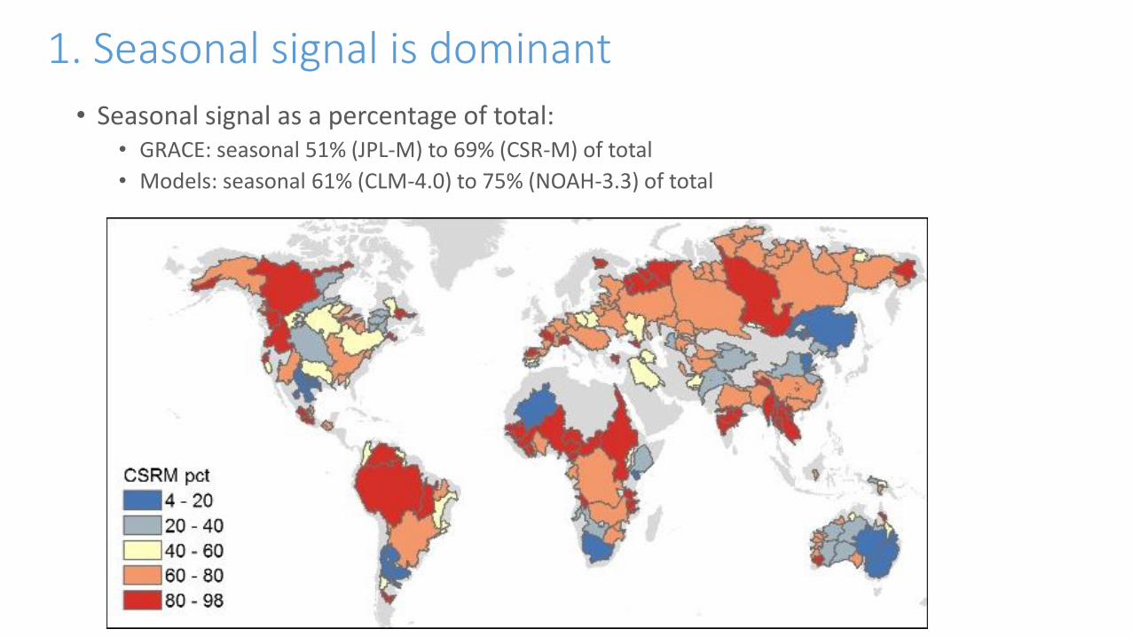
1. Seasonal signal is dominant

• Seasonal signal as a percentage of total: • GRACE: seasonal 51% (JPL-M) to 69% (CSR-M) of total

• Models: seasonal 61% (CLM-4.0) to 75% (NOAH-3.3) of total

1. Seasonal Amplitude in GRACE Mean (CSR, JPL, and GSFC mascons) (peak to peak amplitude)

Objective






2. How do modeled land water storage trends compare with those from GRACE solutions?

Net water storage trends from 2002 - 2014


GRACE: net land water storage trends: 71 – 82 km3/yr

Models: net land water Storage Trend: -450 to -12 km3/yr

-20

-15

-10

-5

0

5

10

km3 /

yr

-80

-60

-40

-20

0

20

40

60

km3/y

r

-20

-15

-10

-5

0

5

10

km3 /

yr

-6

-5

-4

-3

-2

-1

0

1

km3 /

yr

-3

0

3

6

9

12

15

km3 /

yr

Mississippi

Amazon

Okavango

Ganges

Hai

GRACE data GHM LSM

Models

MississippiGRACE Trends ( km3/yr; 2002 – 2014)

Amazon Okavango Ganges

Hai

2. Modeled vs GRACE Land Water Storage Trends

GRACE: CSR-M; JPL-M; CSRT-SH; Models: GHMs: WGHM, PCR-GLOBWB; LSMs: NOAH-3.3; MOSAIC, VIC, CLM-4.0; CLSM-F2.5

GRACE data GHM LSM

1. Global Hydrologic Models relative to GRACE

2. Land Surface Models relative to GRACE

2. Modeled vs GRACE Trends in Total Water Storage

Models underestimate the rises in water storage during wet periods and the declines in water storage during dry periods and related to groundwater abstraction

GRACE rangeGRACE CSR-M

GRACE

WGHMPCR-GLOBWB

GHWRM

NOAH-3.3 MOSAIC VICCLM-4.0CLSM

LSM


2. Model versus GRACE seasonal amplitudesGlobal models simulate seasonal amplitudes much better than trends

WGHM Global Hydrologic Model CLM-4.0 Land Surface Model

y = 0.65x + 36.4R² = 0.61

0

100

200

300

400

500

0 100 200 300 400 500

WG

HM

am

plit

ud

e (m

m)

GRACE mean amplitude (mm)

y = 0.90x + 12.21R² = 0.79

0

100

200

300

400

500

0 100 200 300 400 500

CLM

-4 a

mp

litu

de

(mm

)

GRACE mean amplitude (mm)

2. Ratios in Seasonal Amplitudes between Models and GRACE

GHMs/GRACE mean

2. Ratios in Seasonal Amplitudes between Models and GRACE

GHMs/GRACE mean

LSMs/GRACE mean

2. Variations in Seasonal Amplitudes with Latitude

𝑃𝑒𝑟𝑐𝑒𝑛𝑡 𝐵𝑖𝑎𝑠 =σ𝑖=1𝑛 𝑀𝑜𝑑.−𝑂𝑏𝑠.

σ𝑖=1𝑛 𝑂𝑏𝑠.

𝑥100

2. Variations in Seasonal Amplitudes with Latitude

Comparison of Annual Cycles between Models and GRACE

Objective






2. How does Human Intervention Impact Land Water Storage Trends?

Human intervention:Reservoir storageGroundwater abstractions

WGHM: net water storage change -56 km3/yr


3. How does Human Intervention Impact Land Water Storage Trends?

WGHM: net storage change -56 km3/yr PCR-GLOBWB: net storage change -86 km3/yr

Relative Importance of Climate and Human Intervention in Water Storage in the Colorado River

GW depletion during drought ~ 80% of storage decline, attributed mostly to human water use.

Water storage depletion in U. Colorado Basin related to surfacewater storage and soil moisture + additional groundwater in lower Basin, mostly in response to climate variability.

Relative Importance of Climate and Human Intervention in Colorado Basin

Water storage depletion in U. Colorado Basin related to surface water storage and soil moisture+ additional groundwater in lower Basin, mostly in response to climate variability.

Scanlon et al., WRR, 2015

Scanlon et al., ERL, 2016

Nevada

California

Arizona

CAP: Central Arizona Project

Phoenix AMA

Pinal AMA

Tucson AMA

AMA: Active Management Area

Managed Aquifer RechargeSpreading Basins

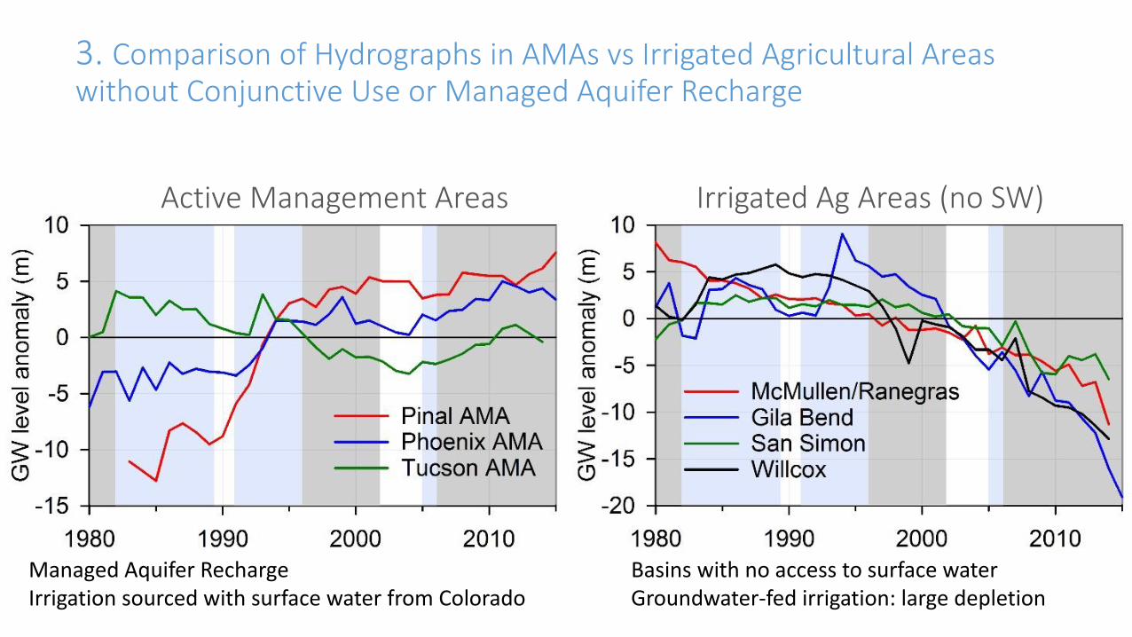
3. Comparison of Hydrographs in AMAs vs Irrigated Agricultural Areas without Conjunctive Use or Managed Aquifer Recharge

Active Management Areas Irrigated Ag Areas (no SW)

Managed Aquifer RechargeIrrigation sourced with surface water from Colorado

Basins with no access to surface waterGroundwater-fed irrigation: large depletion

Net Abstraction of Groundwater

mm/yr

Negative values: increase in groundwater storage as a result of surface water irrigationPositive values: groundwater-based irrigation Döll et al., 2012

3. What is the impact of human intervention on seasonal amplitudes?

Ran global hydrologic models with human intervention (WGHM, PCR-GLOBWB) and without human intervention (NHI: no human intervention). We see very little effect of human intervention (reservoir storage and water abstraction) on seasonal amplitudes at basin scale

Objective






4. What is the impact of land water storage on global mean sea level?

GRACE (H + C)

Human (M)

Climate (GRACE – Human)

GRACE: net trend71 – 82 km3/yr

4. How well can we estimate the net impact of land storage trends on global mean sea level (GMSL) change?

GRACE (H + C)

Human (M)


GRACE: net trend71 to 82 km3/yr

Human intervention-56 to -86 km3/yr

4. How well can we estimate the net impact of land storage trends on global mean sea level (GMSL) change?

GRACE (H + C)

Human (M)


Estimated climate contribution to land water storage = 2 times that from human intervention

GRACE: net trend71 to 82 km3/yr

Human intervention-56 to -86 km3/yr

Objective






5. What is causing differences between models and GRACE? 1. Storage capacity in models: storage compartments and capacity in compartments

a) LSMs: most do not include SWS or GWSb) Underestimation of seasonal amplitudes in tropical basins: lack of surface water

storage and overbank flooding in LSMsc) Storage capacity may not be sufficient to accommodate large declines and rises in

storage

2. Fluxes: Precip. – ET – Roff = DTWSIf models overestimate seasonal amplitude, this may be because they overestimate the input (P), underestimate the output (ET, Roff), or a combination of both.

• Variations in precipitation input • N high latitude basins: snow and frozen soil schemes • Arid basins: overestimation of ET

Path Forward:

• New GRACE Follow On mission launched in May 2018

• Global modeling should consider fluxes and storage

• Use multi-model ensembles rather than relying on single models

• Develop regional models to focus in different areas • Amazon, hotspots of human depletion, N high latitudes

• Calibrate models?

• Use single models and vary processes and parameters to isolate controls on differences

USGS Powell Research Study• Collaboration among USGS, NASA, and academia

• Evaluate global, national, and regional models with GRACE and flux data within the U.S.

Summary


Seasonal signals are dominant, 51 – 75% of total signal, trends ≤ 5% of total signal.


Modeled storage trends underestimate those from GRACE whereas modeled seasonal amplitudes compare more favorably.


Human intervention results in net decline in global water storage (56 – 86 km3/yr) but does not impact seasonal amplitudes at the basin scale.

4. What is the impact of land water storage trends on global mean sea level (GMSL)?

GRACE data indicate net increase in land water storage globally (71 – 82 km3/yr) which contributes negatively to GMSL whereas models indicate decreases in water storage (-450 to -12 km3/yr).


Lack of storage compartments and limited capacity

Uncertainties in fluxes

[email protected]@asch.whigg.ac.cn

Sponsors:

Contact: Bridget Scanlon, Zizhan Zhang

GRACE Products

• Spherical Harmonics (SH) GRACE basin scale data

• Gridded SH GRACE product (Landerer and Swenson, 2012)

• Mascons data (CSR and JPL)

Landerer, F. W., and S. C. Swenson (2012), Accuracy of scaled GRACE terrestrial water storage estimates, Water Resources Research, 48.

Save, H., S. Bettadpur, and B. D. Tapley (2015), Evaluation of global equal-area mass grid solutions from GRACE, European Geosciences Union General Assembly, Vienna, Austria 2015.

Watkins, M. M., D. N. Wiese, D.-N. Yuan, C. Boening, and F. W. Landerer (2015), Improved methods for observing Earth's time variable mass distribution with GRACE using spherical cap mascons, Journal of Geophysical Research-Solid Earth, 120(4), 2648-2671.

Scanlon, B. R., Z. Zhang, H. Save, D. N. Wiese, F. W. Landerer, D. Long, L. Longuevergne, and J. Chen (2016), Global evaluation of new GRACE mascons products for hydrologic applications, Water Resour. Res. , 52(12), 9412-9429.

Processing Spherical Harmonic GRACE Data

• Raw GRACE KB range rate data, noisy

• It takes ~ 90 mins for satellite to complete circum-polar orbit, need 1 month to get global coverage

• Spherical Harmonics processing: Remove high frequency noise (truncation and filtering), also removes signal• Restore signal (scaling factors)

• Apply same processing to land surface model as GRACE to estimate a scaling factor: Land surface model soil moisture storage – Truncation + Filtering = LSMTF

• Scaling factor (dimensionless)= LSM/ LSMTF (≥ 0)

• Mascons: no scaling factor used for CSR GRACE data; NASA JPL use scaling factor to downscale 3 degree data to 1 degree data based on LSMs.

Recent Studies

• Model Intercomparison Projects (MIPs) based on fluxes (river discharge and evapotranspiration) have shown that global hydrologic models are even more variable than climate models (Schewe et al., PNAS, 2014) (InterSectoral Impact Model Intercomparison Project, ISIMIP)

• GRACE data show net increase in land water storage over past decade in response to climate variability (Reager et al., Science, 2016)

• GRACE satellites provide the big picture

Differences between Spherical Harmonics and Mascons• SH analysis: represents global mass change, cannot distinguish land

and ocean, leakage effects

• Mascons (mass concentration blocks), regional or global analysis, can delineate oceans and land• Higher signal/noise ratio than SH

• Can check for signal loss by doing post fit residuals against original GRACE range rate data

• All signal captured within GRACE resolution

• Some solutions use no models (Univ. Texas Center for Space Research) and others use models for downscaling 3 deg gridded data (NASA JPL mascons)

2. Long-term trends in Total Water Storage


2. Long-term trends in Total Water StorageWater Storage?


Richey et al., 2015Third of big GW basins under distress

California drought

GRACE satellite data versus ground-based monitoringNov. 16, 2014

comparison of land water storage from global hydrologic and … · 2018-09-07 · comparison of...

Documents