Hydrologic data assimilation NSF workshop Oklahoma

Dr Damian Barrett

CSIRO Land & Water

23 October 2007

CSIRO. Hydrologic Forecasting

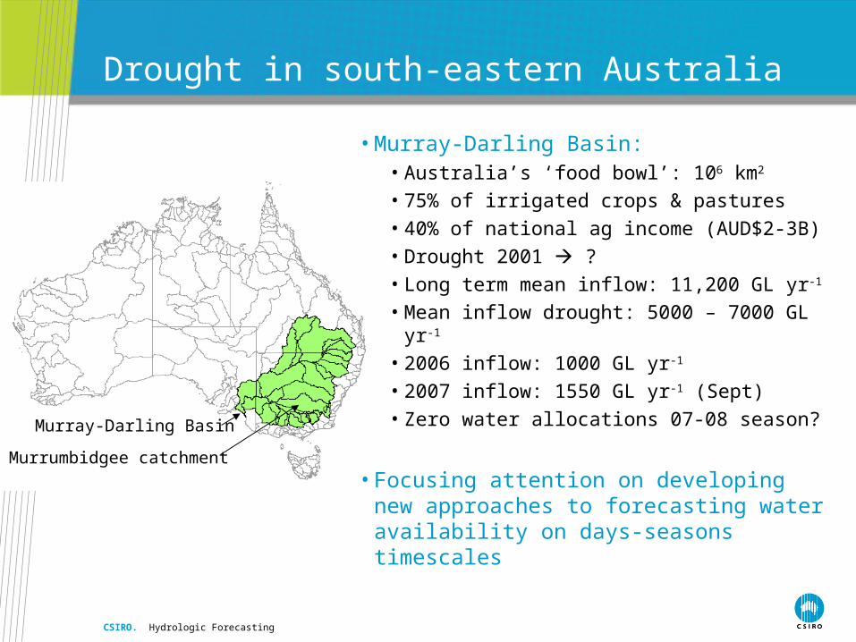
Drought in south-eastern Australia

Murray-Darling Basin

Murrumbidgee catchment

• Murray-Darling Basin:• Australia’s ‘food bowl’: 106 km2

• 75% of irrigated crops & pastures

• 40% of national ag income (AUD$2-3B)

• Drought 2001 ?

• Long term mean inflow: 11,200 GL yr-1

• Mean inflow drought: 5000 – 7000 GL yr-1

• 2006 inflow: 1000 GL yr-1

• 2007 inflow: 1550 GL yr-1 (Sept)

• Zero water allocations 07-08 season?

• Focusing attention on developing new approaches to forecasting water availability on days-seasons timescales

CSIRO. Hydrologic Forecasting

Hydrologic forecasting

• A Definition:

The prediction of hydrologic state variables (rainfall, ET, SMC, runoff, drainage, stream flow…) at future time based on the evolution of those variables in time (model) and conditioning those variables with observations while considering the relative uncertainties of model and observations

MODEL STATES ANALYSIS STATES FORECAST

OBSERVATIONS

CSIRO. Hydrologic Forecasting

Role of satellite observations

• Polar orbiting moderate resolution satellite sensors: • Whole earth coverage at high temporal frequency

• Spatial infilling (gaps between in situ gauges & instruments)

• Multiple sensors: Different & independent ‘viewpoint’ in space/time/wavelength

• Remote Sensing: information on radiometric properties of surface

• Two challenges:• Relate observations to hydrologic state variables while quantifying

errors and removing biases

• ‘Synthesise’ data from multiple sensors to yield optimal estimates of relevant state variables

CSIRO. Hydrologic Forecasting

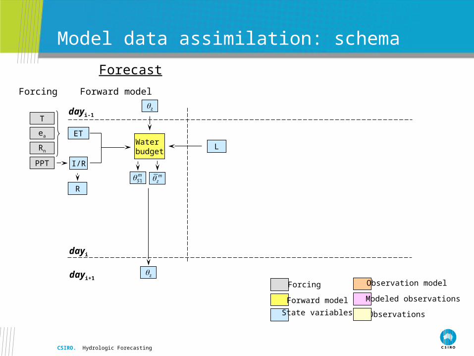
Model data assimilation: schema

Forecast

L

z

Water budget

z

dayi

dayi+1

dayi-1

Observations

Forcing

Forward model

State variables

Observation model

Modeled observations

Forcing Forward model

PPT I/R

R

ET

T

ea

Rn

1mS m

z

CSIRO. Hydrologic Forecasting

0 100 200 300 400 500 6000

50

100

150

200

250

300

0 100 200 300 400 500 6000

50

100

150

200

250

300

0 100 200 300 400 500 6000

50

100

150

200

250

300

Model data assimilation: schema

Op RT-1

,r n

AnalysisForecast

J

L

z

Water budget

z

dayi

dayi+1

dayi-1

Observations

Forcing

Forward model

State variables

Observation model

Modeled observations

Forecast

Forcing ObservationsForward model 3D Variational Assimilation

TS

PPT I/R

R

ET

T

ea

Rn

SEB

Microwave RT TBJ

TV TSS

ampl

ing/

inte

rpol

atio

n S zT

1B ST

1aS a

z1aS a

z

1mS m

z

CSIRO. Hydrologic Forecasting

3D variational assimilation

• Cost-function: a metric of ‘distance’ between model and observations in state space

1 1a a a b a bJ H H y x R y x x x B x x

ˆH x y

R = covariance matrix of observation errorsB = covariance matrix of model errorsxa = analysis state vectorxb = ‘background’ vector of model states

‘Observation operator’

• Benefits: gradient search (no inversions) and sequential (imagery)• Expensive: requires re-evaluation of H every iteration

CSIRO. Hydrologic Forecasting

3D variational assimilation

• H is the ‘tangent linear operator’: fixed providing xb – xa is ‘small’

• Requires evaluation of H and construction of once only

1 1b a b b a b a b a bJ H H y x H x x R y x H x x x x B x x

1 1a a a b a bJ H H y x R y x x x B x x

1 1

2 2

1 2

1 2

x x

x x

H H

x x

H H

x x

H

Taylor expansion of observation model

CSIRO. Hydrologic Forecasting

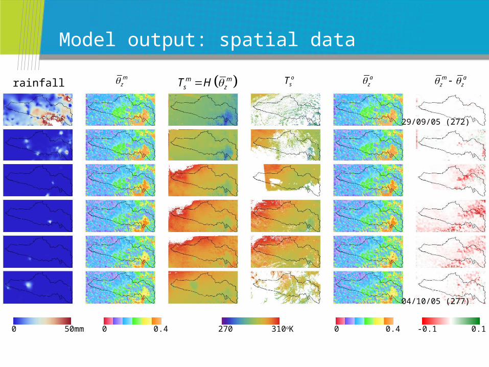
Model output: spatial data

• D

0 50mm 0 0.4 0 0.4270 310oK -0.1 0.1

rainfallmz o

sTaz m a

z z m ms zT H

29/09/05 (272)

04/10/05 (277)

CSIRO. Hydrologic Forecasting

Model output: comparison with stream flow

0

5000

10000

15000

20000

0 5000 10000 15000 20000

Observed peak flow (ML/day)

Mod

elle

d p

eak

flow

(M

L/da

y)

r2 = 0.85

48

47

61

57

38

33

44

0

500

1000

1500

250 255 260 265 270 275 280 285

model peak flow

derived peak flow

0

500

1000

1500

2000

250 255 260 265 270 275 280 285

stream flow

derived base flow

Flo

w (

ML

/da

y)

Gauge #33

Model

Obs

CSIRO. Hydrologic Forecasting

Challenges

• Models• Coupling models operating at different scales while dealing with

non-linearities and heterogeneity

• Inadequate physics in forward and observation models

• Quantifying errors in model

• Efficient optimisation of massive problems

• Modelling at a scale relevant to decision making

• Observations• Gaps in observations (drift by model)

• Key data sets and improve QA

• Quantifying errors in observations

• Representivity, scaling and aggregation errors: matching observations and model variables that differ in time/space scale

Contact UsPhone: 1300 363 400 or +61 3 9545 2176

Email: enquiries@csiro.au Web: www.csiro.au

Thank you

CSIRO Land and Water Dr Damian BarrettResearch Group Leader – Remote sensingPhone: 02 6246 5558Email: Damian.Barrettt@csiro.auWeb: www.csiro.au/group