Agricultural Engineering Research Journal 2 (3): 43-54, 2012ISSN 2218-3906 © IDOSI Publications, 2012DOI: 10.5829/idosi.aerj.2012.2.3.76

Corresponding Author: Nazila Sedaei, Sari University of Agriculture and Natural Resources, P.o.Box 737, Sari-Iran.

43

Comparison of Empirical Methods and Neural Network Technique in Predication ofSuspended Sediment: a Case Study of Armand River, Karoon Basin, Iran

Nazila Sedaei and Kaka Shahedi1 2

Sari University of Agriculture and Natural Resources, P.o.Box 737, Sari-Iran1

College of Natural Resources, Sari Agricultural Sciences and Natural Resources University2

Abstract: Prediction of suspended sediment discharge in rivers is an important process for water resourcesimprovement and managements. In practice sediment yield is usually calculated from direct measurement ofsediment concentration of river or indirectly using sediment transport equations. Since direct measurementcannot be performed for all stream gauges, indirect methods are preferred. In this study, predictions ofsuspended sediment load for Armand River in Iran using selected empirical equations were made based on 772sets of data. This research examines whether a neural network technique (MLP) can predict the suspendedsediment discharge in the river better than the empirical formulae such as Toffaleti, Chang-Simons-Richardson,Einstein, Lane-Kalinske, Brooks and Bagnold. The results showed that MLP has good performance to estimatesuspended sediment in comparison with aforementioned equations. The results revealed that MLP usingvelocity, area, depth, hydraulic ratio as input parameters and also considering 4 units in input layer, 2 inhidden layer and 1 in output layer shows the best performance among all of the models of neural network.Evaluation of the results showed RMSE=0.027 and R = 0.90, which is recorded the highest determination2

coefficient.

Key words: Empirical methods Artificial Neural Network Armand River Iran

INTRODUCTION very lengthy and costly. Because of this, some formulae

Improving knowledge on suspended sediment estimate the sediment load in rivers [6]. Shirin and Kisi [7]yields, dynamics and water quality is one of current applied convenient Gene Expression Programming (GEP),major environmental challenges addressed to scientists Nero-Fuzzy (NF) and Artificial Neural Network (ANN)and hydropower managers [1]. Indeed, estimates of techniques and compared with each other. Comparison ofsuspended sediment load are essential to investigate results indicated that the wavelet conjunction modelsabout river transportation. Especially the time and the significantly increased accuracy of single GEP, NF andrelation between time and suspended sediment discharge ANN models in suspended sediment estimation. Kisi [8]are important because the depletion and increasing in the demonstrated the evidence of ANN ability in Daily Riversediment amount occur during flood seasons [2] and also suspended sediment concentration modeling. BesideChen et al. [3] found that the fine suspended sediment these methods, sediment rating curve showed goodconcentrations had pronounced seasonal and spring- results in predication of suspended sediment for 3 daysneap tidal variations. Although the existence of ahead [9]. Bisantino et al. [10] have compared thesuspended sediment causes a lot of problems in rivers but field data with those predicted from four formulaein contrast there are some agricultural hills slope (Ackers-White, Engelund-Hansen, Yang and Van Rijn).maintenance practices which can modify sediment erosion They illustrated that for low sediment loads, thein the basin and in the future in rivers [4]. Estimation of formulae results are not reliable or at least less reliable.sediment load is required in practical studies for the Nourani et al. [11] developed two ANN models forplanning, designing, operation and maintenance of water semi-distributed modeling of suspended sediment loadresources structures [5]. The sediments transportation process of the Eel River watershed located in California,monitoring requires a good sampling technique which is USA. The results demonstrate that although the predicted

were developed from 1950 up to now to predict and

Agric. Engineering Res. J., 2(3): 43-54, 2012

44

sediment load time series by both models are in calculations of sediment load are based on continuoussatisfactory agreement with the observed data, the discharge and turbidity records, the latest calibrated withgeomorphologic ANN model performs better than direct suspended sediment sampling that covered theintegrated model because of employing spatially whole range of observed hydraulic conditions. Gao [20]variable factors of the sub-basins as the model's inputs. found that in practice, the empirical equation can be usedTherefore, the model can operate as a non-linear to estimate the maximum possible bed-load transporttime-space regression tool rather than a fully lumped rates during high flow events, which is useful for variousmodel. Based on the results of Cobaner et al. [12] the sediment-related river managements. Kisi [13] comparedNero-Fuzzy models perform better than the other methods three methods of neural network with each other and thesuch as empirical ones in daily suspended load results indicated that the NDE models give betterestimation. On the other hand, what Kisi [13] showed in estimates for suspended sediment in river than NF, NNhis research which proposed Neural Differential and RC techniques. In this research, predictions ofEvolution (NDE) models to estimate suspended sediment suspended sediment for Armand river located inconcentration in river is not consistent with [12]. Chahar-Mahal-Bakhtiari Province were made and analyzedThe emergence of ANN technology has given many using the selected empirical equations and NN techniquepromising results in the field of hydrology and water and also the results were compared with each other theresources and also sediment hydraulics to solve the same as what Roushangar et al. [21] have done in theirnonlinear system complexity problem [14, 15]. study.The hydrological characteristics of the river such asspatio-temporal changes of sediment concentrations and MATERIALS AND METHODSdifficulties for their estimation encouraged using theANN models. Rai and Mathur [16] in his research about Study Area: Application of six suspended sedimentmodeling sediment load during storm events found the estimation formulae was tested in Armand River in Iran.Neural Network technique as a suitable estimation tool Sediment discharge and sediment concentration and alsoin two catchments in the USA. One of the most different flow discharges series for the stations are used toresearches that were done by Cigizoglu and Kisi [17] develop and verify models' performances. Armand Stationapproved the higher performance of Range-Dependent is located in Armand River at 50° 46' Latitude 31° 40'Neural Network (RDNN) in comparison with conventional Longitude. The drainage area of this river is about 9986ANN applications. Most of the studied transport models km and the station that these data are used from, isare based on simplified assumptions that are valid in ideal located in 1082 m height. This river is located in NorthLaboratory conditions only and may not be true for much Karoon Basin. The basin is one part of Zagroscomplicated natural river systems. Models based on more mountainous lands and is covered by limestone and marlsophisticated theoretical solutions require a large number soils and semi-dense forests. The mean annual rainfall ofof parameters that are impossible or difficult to collect for the basin is about 500 mm. Fig. 1 shows the location ofa natural river system [18]. Tena et al. [19] found that study area in Iran.

2

Fig. 1: The location of study area in Iran.

yu

*f

ouS

=

sKX

∆ =

u

Agric. Engineering Res. J., 2(3): 43-54, 2012

45

Table 1: Descriptions of abbreviations which are used in suspended sediment formulae.

Abbreviations descriptions

1 The average local velocity at distance y from the bed

2 The shear velocity

3 S The density of the waterf

4 S The slope of the energy grade linee

5 R The hydraulic radius

6 g The acceleration due to gravity

7 y The distance from the bed

8 v The kinematic viscosity of the water

9 K The roughness of the beds

10 x A corrective parameter

11 The apparent roughness of the surface

12 The thickness of the laminar sub layer of a smooth wall

13 g The acceleration due to gravity

14 y The distance from the bed

15 k Van-Karman coefficient equal to 0.4

16 The fall velocity

17 q The flow discharge

18 q The suspended sediment dischargesw

19 C As the suspended sediment concentration in water depth aa

20 S Assumed as the ratio of water density to sediment densityg

21 The mean velocity

22 The shear stress

23 q The sediment dischargesm

24 S The bed slope

Data Sources: The range of all data used in this study lie processing system that has certain performancewithin the range of data used in the development of the characteristics resembling to the biological arrangementselected equations. This is illustrated in Table 1. A 44 of Neurons in human brain [22]. An ANN establishes ayears (1967-2009) data was collected for the study area. data-driven nonlinear relationship between inputs andAbnormal distribution of data have such effects that outputs of a system [23]. Thus, Neural Networks (NN) hasmay lead to high fluctuations in figures and reduces the been successfully applied in a number of diverse fieldsreliability of analytical results, thus normalization of data including water resources. In the hydrological forecastingis necessary. At first step imperfect data were eliminated context, (ANNs) may offer a promising alternative forand then the missing data were estimated using rainfall–runoff modeling [24, 25-27], stream flow predictioninterpolation method. [28,17, 29-32]. There are few published studies in the

The river under study is categorized as a small river field of suspended sediment prediction using artificialwith aspect ratio more than 5. Data covers flow velocities intelligence methods such as neural networks and fuzzyfrom 0.66 m/s to 4.12 m/s and flow depths from 0.91 logic approaches. Tayfur [33] reviewed the ANN-basedto 1.5 m. modeling in hydrology over the last years and reported

Artificial Neural Networks: Artificial Neural Network multi-layer Feed-forward Neural Networks (FNN) trained(ANN) is a massively parallel-distributed information by the standard Back

that about 90% of the experiments extensively use the

' 2

2 1

2

1

( )

1

( )

N

i iiN

ii

y yr

y y

=

=

−

= −

−

∑

∑

' 2

2 1

2

1

( )

1

( )

N

i iiN

ii

y yR

y y

=

=

−

= −

−

∑

∑

y

* ( )syKU D yD

= −

1/ 2*(1 )KD U −

zy

a

C d y aC y d a

−= −

*0.4szu

=

Agric. Engineering Res. J., 2(3): 43-54, 2012

46

Propagation (BP) algorithm. Maier and Dandy [34] Where d is the difference between ith estimated andreviewed 43 articles dealing with use of the ANN model ith observed values of suspended sediment concentrationfor estimation of water resources variables. and N is the number of observations. The coefficient of

The neural network typically consists of an input determination used to evaluate the performance of thelayer, an output layer and a layer of nonlinear processing models is defined as:elements, known as the hidden layer. The ANN hasseveral algorithms used in forecasting and modeling (2)processes. In this study, the feed forward backpropagation algorithm was selected for modeling thesuspended sediment concentration. The most commonlyused ANN in hydrological predictions is the BP algorithm[35]. BP is a supervised learning technique used fortraining the neural networks. Basically, it is a gradientdescent technique to minimize some error criteria. The BPnetwork structure in this study includes a three-layerlearning network consisting of an input layer, a hiddenlayer and an output layer.

Improving the Generalization Level in Model:One of the most important and effective problemsthat occurs during neural network training is overfitting. The error on the training set is driven to a verysmall value, but when new data is presented to thenetwork, the error is large. The network has memorizedthe training examples, but it has not learned togeneralize to new situations [36]. The feed forward backpropagation algorithm is a widely applied three layersnetwork type consisting of an input layer, a hiddenlayer and an output layer. The determination of thenumber of nodes in a hidden layer providing the besttraining results was the initial process of the trainingprocedure. The suspended sediment concentrationestimation was carried out with the BP throughconsidering the width and depth and also the area of theriver, river discharge and velocity as associate inputs ofthe network. Various hidden nodes numbers were tried forthe BP algorithm.

Model Evaluation: The performances evaluation criteriawere the root mean square errors (RMSE) and thecoefficient of determination (R ) expressed between2

estimated and observed suspended sedimentconcentration as:

(1)

i

Where y and y are the ith observed (actual) andi i

estimated values of y and is the mean of the observed

values of y; and N is the number of observations.

Suspended Sediment Formulae: The finer particles of thesediment load of streams move predominantly assuspended load. Suspension as a mode of transport isopposite to what Chang_Simons_Richardson [37]called surface creep and to what they refined as theheavy concentration of motion immediately at the bed.In popular parlance this has been called bed load,although as defined in this publication bed load includesonly those grain sizes of the surface creep which occur insignificant amounts in the bed.

Chang-Simons-Richardson [37] derived a sedimenttransport model in which, they assumed the belowformula valuable

(3)

And also defining the amount of equal ands

introducing =y/D, shear stress may be

determined as; c the concentration in water depth y, isy

estimated as;

(4)

In which the concentration of these particles at y isc . y is the variable of integration, the dimensionlessy

distance of any point in the vertical from the bed,measured in water depth d, with;

(5)

( )

21/ 2

1 1/ 21 1

z

a

a a

C AC

= − −

*1 2

2sw a

Uq DC VI IK

= −

2( 1) 0.01 ( / )g sm sg S q u− =

1*

( , , )swB

md

q VT k Z EC q U

=

i

Z

VZiC RS

=

Agric. Engineering Res. J., 2(3): 43-54, 2012

47

Fig. 2: Basic concepts of artificial neuron (after Yang, Fig. 4: I vs. a ( in water depth a) to determine the2009). amount of I for individual depths (Yang, 1940).

Fig. 3: I vs. a ( in water depth a) to determine1

the amount of I for individual depths Brooks [39] derived a sediment transport model in1

(Yang, 1940). which he takes the Semi-logarithmic velocity distribution

Also replacing Equation (3) in Equation (4), Equation sediment discharge depends on suspended sediment6 would be obtained: concentration. The suspended sediment rate can be

(6)

The suspended sediment discharge would be where Z , is a function of estimated in the form of

(7)

In this equation there are two factors I and I that can basically the description of the velocity distributions1 2

be obtained either from the graphs I - (Fig. 3) or and of the frictional loss for turbulent flow.1

I - (Fig. 4). Einstein has found that in describing sediment2

The performance of Chang-Simons-Richardson to transport the velocity distribution in open-channelestimate the suspended sediment is evaluated using flow over a sediment bed is best described byRMSE and R . the logarithmic formulas based on V. Karman's2

2

2

Bagnold [38] derived a stream-based sedimenttransport model. In that model, Bagnold assumes thesediment is transported in two modes, i.e., the bed loadtransport and the suspended transport. The bed loadsediment is transported by the flow via grain to graininteractions; the suspended sediment transport issupported by fluid flow through turbulent diffusion.The suspended sediment rate can be calculated usingthe below formula [3];

(8)

into account and also determined that suspended

calculated as:

(9)

1

C is the factor which depends on temperature.z

E=e and C is the suspended sediment-(kv/U*)-1md

concentration in y=D/2 numbers.The hydraulics of uniform flow includes

( )* *10 10

*5.50 5.75log 5.75log 9.05yu yu yu

u = + =

10 10*

8.50 5.75log ( ) 5.75log (30.2 )y

s

u y yu k k

= + =

10 10*

5.75log (30.2 ) 5.75log (30.2 )y

s

u Vx yu k

= =∆

* 105.75 log (30.2 / )d d z

y y ay y

d y aC u dy C u y dyy d a

−= ∆ − ∫ ∫

* ( )sykU D yD

= −

20 *2

0

( )

D

s D

s

dykU yD y dy

D D= = −∫

∫

La

CPC

=

*

15expsw a Laq qC P

U D

=

(1 ) ( / ) vvU V Y R= +

0.1198 0.00048v FT= ×

i

Z

VZiC RS

=

260.67 0.0667Z FC T= −

1 10.244 0.5

1

( /11.24) ( / 2.5) ( / 2.5)Zi Zi

SUiR R R R

q Mi − =

2 20.244

2

( /11.24) ( / 2.5) ( /11.24)Zi

SmiR R R

q Mi − =

3 3

3

( /11.24) (2 )SLi

R diq Mi −=

Agric. Engineering Res. J., 2(3): 43-54, 2012

48

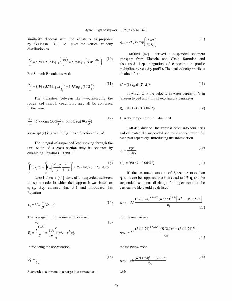
similarity theorem with the constants as proposed (17)by Keulegan [40]. He gives the vertical velocitydistribution as

(10) transport from Einstein and Chain formulae and

For Smooth Boundaries And: obtained from

(11) (18)

The transition between the two, including the relation to bed and is an explanatory parameter rough and smooth conditions, may all be combinedin the form: (19)

(12) T is the temperature in Fahrenheit.

subscript (x) is given in Fig. 1 as a function of k / . and estimated the suspended sediment concentration fors

The integral of suspended load moving through theunit width of a cross section may be obtained by (20)combining Equations 10 and 11.

(13) (21)

Lane-Kalinske [41] derived a suspended sediment so it can be supposed that it is equal to 1/5 and thetransport model in which their approach was based on suspended sediment discharge for upper zone in the

= , they assumed that =1 and introduced this vertical profile would be defineds m

Equation

(14)

The average of this parameter is obtained For the median one (15)

Introducing the abbreviation for the below zone

(16) (24)

Suspended sediment discharge is estimated as: with

Toffaleti [42] derived a suspended sediment

also used deep integration of concentration profilemultiplied by velocity profile. The total velocity profile is

in which U is the velocity in water depths of Y inv

F

Toffaleti divided the vertical depth into four parts

each part separately. Introducing the abbreviation

If the assumed amount of Z become more thani

v, v

(22)

(23)

0.75643.2 (1 ) Li

ZiPi VCMiR −

+=

1 1 1.5v Zi= + −

2 1 v Zi= + −

3 1 1.756v Zi= + −

Agric. Engineering Res. J., 2(3): 43-54, 2012

49

(25) The Neuron in the output layer represents

and in the hidden layers was determined by a trial-and-error

(26) variables. In this study, 20 input combinations, which fell

(27) different groups were designed to compare the

(28) those in the same group were designed to examine the

In Equation 25, P is the percentage of inputs and the outputs. The network in group 1 used thei

sediments with d diameter; C must be calculated for width of the river beside other parameters in each subi Li

each diameter in water depths Y. Total suspended group. In this group the second sub group with threesediment load discharge per unit in the river would be input parameters has the best simulation in comparisonequal with all suspended sediment load discharges in with others. Among all of the simulations in Table 2, it canthe parts. be recognized that in the 9 and 5 and also 8

RESULTS AND DISCUSSION an output. In addition individuals were tested and it was

A difficult task with MLP is choosing the number of Evaluation of this simulation showed that velocity, area,nodes in each of the layer. There is no theory yet to depth and hydraulic ratio, flow discharge, width and alsodetermine that how many hidden units must be velocity, area, depth, flow discharge considered withinconsidered for each function. In this study, the three layer two groups can simulate the sediment discharge withMLP is used and common trial and error method is used RMSE equal 0.032 and 0.027, respectively. Alsoto select the number of nodes, specially the hidden determination coefficient was equal 0.81 and 0.90 for eachnodes. The input data were standardized before being group, respectively (Fig. 2; the best network in suspendedentered to the model. The sediment concentration data sediment discharge). During the training process the bestwere also normalized in the same way. After training step, results were determined with the optimization function asthe weights were saved and used to test data for each gradient descent and momentum equal to 0.9 and alsoneural network and also models. interval offset equal to 0.5.

suspended sediment flux (Fig. 2). The number of Neurons

method. Neurons in the input layer represent input

in four groups, were used (Table 2). The networks in

performances of different sets of causal variables; while

degree of number of the parameters effect between the

th th th

subgroups, there is the most ability to simulate the flux as

seen that W lonely has good ability to predict Q .s

Table 2: Performance of MLP as a neural network.Network Type Decoration RMSE R2

W Q (2 1 1) 0.081 0.32w

W Q V (3 4 1) 0.067 0.51w

W Q V A (4 1 1) 0.066 0.54w

W Q V A D (5 1 1) 0.066 0.55w

W Q V A D RH (6 1 1) 0.032 0.81w

Q V (7 1 3) 0.057 0.62w

Q V A (2 3 1) 0.056 0.64w

Q V A D (3 1 1) 0.044 0.79w

Q V A D RH (4 2 1) 0.027 0.90w

V A (5 5 1) 0.049 0.67V A D (6 1 1) 0.042 0.68V A W (2 1 1) 0.053 0.67V A D RH (3 3 1) 0.059 0.58A Qw (3 1 1) 0.077 0.46A D (4 2 1) 0.042 0.68A W (5 3 1) 0.042 0.68A D RH (2 2 1) 0.042 0.68D RH (2 4 1) 0.041 0.69D W (2 5 1) 0.040 0.70D Qw (3 3 1) 0.066 0.54

Agric. Engineering Res. J., 2(3): 43-54, 2012

50

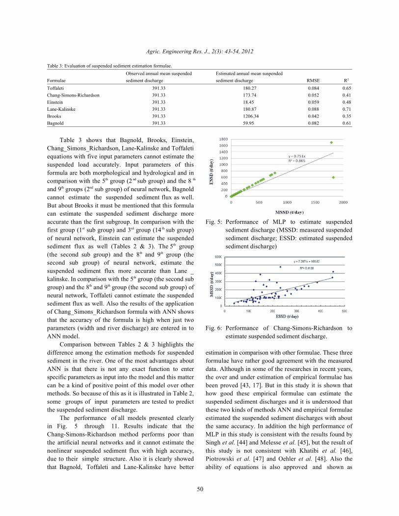
Table 3: Evaluation of suspended sediment estimation formulae.Observed annual mean suspended Estimated annual mean suspended

Formulae sediment discharge sediment discharge RMSE R2

Toffaleti 391.33 180.27 0.084 0.65Chang-Simons-Richardson 391.33 173.74 0.052 0.41Einstein 391.33 18.45 0.059 0.48Lane-Kalinske 391.33 180.87 0.088 0.71Brooks 391.33 1206.34 0.042 0.35Bagnold 391.33 59.95 0.082 0.61

Table 3 shows that Bagnold, Brooks, Einstein,Chang_Simons_Richardson, Lane-Kalinske and Toffaletiequations with five input parameters cannot estimate thesuspended load accurately. Input parameters of thisformula are both morphological and hydrological and incomparison with the 5 group (2 sub group) and the 8th nd th

and 9 groups (2 sub group) of neural network, Bagnoldth nd

cannot estimate the suspended sediment flux as well.But about Brooks it must be mentioned that this formulacan estimate the suspended sediment discharge moreaccurate than the first subgroup. In comparison with the Fig. 5: Performance of MLP to estimate suspendedfirst group (1 sub group) and 3 group (14 sub group) sediment discharge (MSSD: measured suspendedst rd th

of neural network, Einstein can estimate the suspended sediment discharge; ESSD: estimated suspendedsediment flux as well (Tables 2 & 3). The 5 group sediment discharge)th

(the second sub group) and the 8 and 9 group (theth th

second sub group) of neural network, estimate thesuspended sediment flux more accurate than Lane _kalinske. In comparison with the 5 group (the second subth

group) and the 8 and 9 group (the second sub group) ofth th

neural network, Toffaleti cannot estimate the suspendedsediment flux as well. Also the results of the applicationof Chang_Simons_Richardson formula with ANN showsthat the accuracy of the formula is high when just twoparameters (width and river discharge) are entered in to Fig. 6: Performance of Chang-Simons-Richardson toANN model. estimate suspended sediment discharge.

Comparison between Tables 2 & 3 highlights thedifference among the estimation methods for suspended estimation in comparison with other formulae. These threesediment in the river. One of the most advantages about formulae have rather good agreement with the measuredANN is that there is not any exact function to enter data. Although in some of the researches in recent years,specific parameters as input into the model and this matter the over and under estimation of empirical formulae hascan be a kind of positive point of this model over other been proved [43, 17]. But in this study it is shown thatmethods. So because of this as it is illustrated in Table 2, how good these empirical formulae can estimate thesome groups of input parameters are tested to predict suspended sediment discharges and it is understood thatthe suspended sediment discharge. these two kinds of methods ANN and empirical formulae

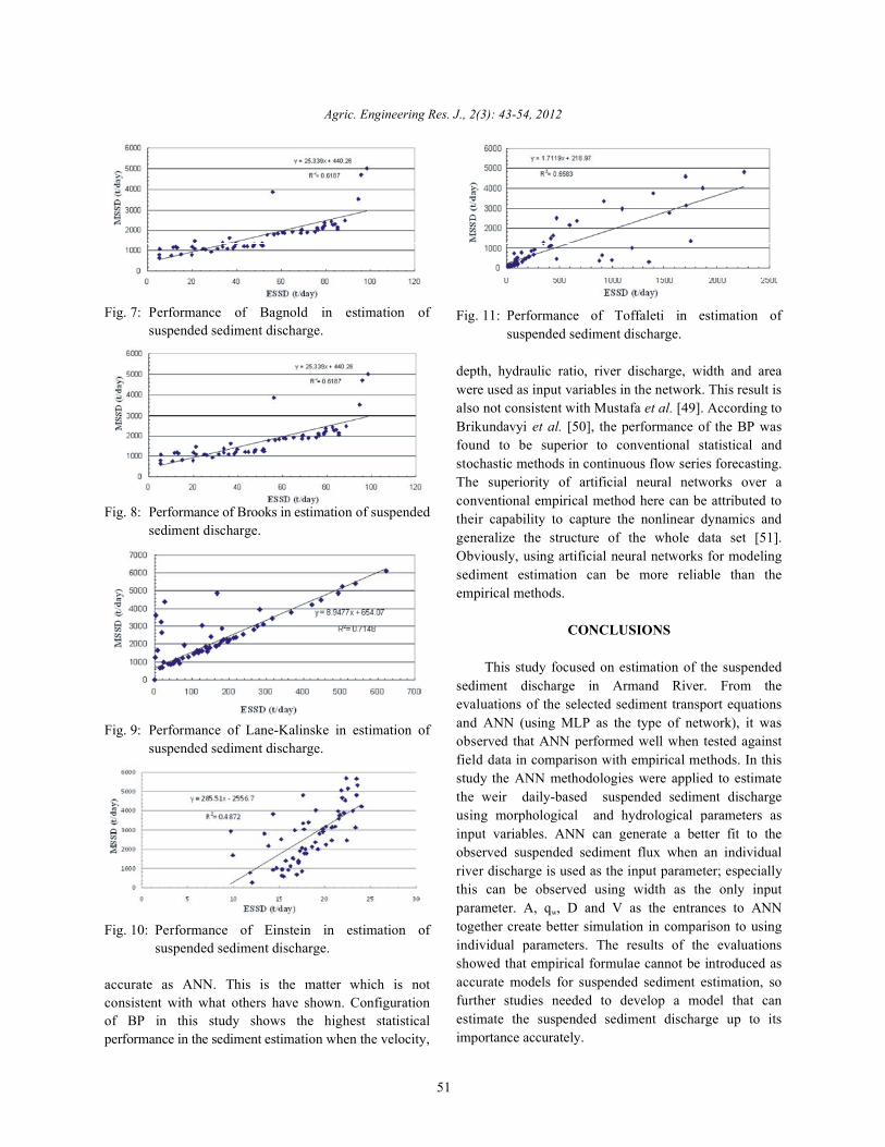
The performance of all models presented clearly estimated the suspended sediment discharges with aboutin Fig. 5 through 11. Results indicate that the the same accuracy. In addition the high performance ofChang-Simons-Richardson method performs poor than MLP in this study is consistent with the results found bythe artificial neural networks and it cannot estimate the Singh et al. [44] and Melesse et al. [45], but the result ofnonlinear suspended sediment flux with high accuracy, this study is not consistent with Khatibi et al. [46],due to their simple structure. Also it is clearly showed Piotrowski et al. [47] and Oehler et al. [48]. Also thethat Bagnold, Toffaleti and Lane-Kalinske have better ability of equations is also approved and shown as

Agric. Engineering Res. J., 2(3): 43-54, 2012

51

Fig. 7: Performance of Bagnold in estimation ofsuspended sediment discharge.

Fig. 8: Performance of Brooks in estimation of suspendedsediment discharge.

Fig. 9: Performance of Lane-Kalinske in estimation ofsuspended sediment discharge.

Fig. 10: Performance of Einstein in estimation ofsuspended sediment discharge.

accurate as ANN. This is the matter which is notconsistent with what others have shown. Configurationof BP in this study shows the highest statisticalperformance in the sediment estimation when the velocity,

Fig. 11: Performance of Toffaleti in estimation ofsuspended sediment discharge.

depth, hydraulic ratio, river discharge, width and areawere used as input variables in the network. This result isalso not consistent with Mustafa et al. [49]. According toBrikundavyi et al. [50], the performance of the BP wasfound to be superior to conventional statistical andstochastic methods in continuous flow series forecasting.The superiority of artificial neural networks over aconventional empirical method here can be attributed totheir capability to capture the nonlinear dynamics andgeneralize the structure of the whole data set [51].Obviously, using artificial neural networks for modelingsediment estimation can be more reliable than theempirical methods.

CONCLUSIONS

This study focused on estimation of the suspendedsediment discharge in Armand River. From theevaluations of the selected sediment transport equationsand ANN (using MLP as the type of network), it wasobserved that ANN performed well when tested againstfield data in comparison with empirical methods. In thisstudy the ANN methodologies were applied to estimatethe weir daily-based suspended sediment dischargeusing morphological and hydrological parameters asinput variables. ANN can generate a better fit to theobserved suspended sediment flux when an individualriver discharge is used as the input parameter; especiallythis can be observed using width as the only inputparameter. A, q , D and V as the entrances to ANNw

together create better simulation in comparison to usingindividual parameters. The results of the evaluationsshowed that empirical formulae cannot be introduced asaccurate models for suspended sediment estimation, sofurther studies needed to develop a model that canestimate the suspended sediment discharge up to itsimportance accurately.

Agric. Engineering Res. J., 2(3): 43-54, 2012

52

ACKNOWLEDGEMENTS 9. Mizumura, K., 2011. Prediction of Sediment

This paper is primarily the result of the analysis ofthe first author during her Ph.D. study at Sari Universityof Agricultural Sciences and Natural Resources.The author would also gratefully acknowledge thehelp rendered by her Professors in the University.The anonymous reviewers are highly appreciated fortheir instructive comments and suggestions.

REFERENCES

1. Owens, P.N., R.J. Batalla, A.J. Collins, B. Gomez,D.M. Hicks, A.J. Horowitz, G.M. Kondolf,M. Marden, M.J. Page, D.H. Peacock, E.L. Petticrew,W. Salomons and N.A. Trustrum, 2005. Fine-grainedsediment in river systems: environmentalsignificance and management issues. River ResAppl., 21: 693-717.

2. Picouet, C., B. Hingray and J.C. Olivry, 2001.Empirical and conceptual modeling of thesuspended sediment dynamics in a large tropicalAfrican river: the Upper Niger River basin. J. Hydro.,250(1-4): 19-39.

3. Chen, S.L., G.A. Zhang, S.L. Yang and J.Z. Shi, 2006.Temporal variations of fine suspended sedimentconcentration in the Changjiang River estuary andadjacent coastal waters, China, Water Resources inRegional Development: The Okavango River. JHydro., 331(1-2): 137-145.

4. Ranzi, R., T.H. Le and M.C. Rulli, 2011. A RUSLEapproach to model suspended sediment load in theLo River (Vietnam): effects of reservoirs and landuse changes. J. Hydro., In Press.

5. Altunkaynak, A., 2009. Sediment loadprediction by genetic algorithms. Adv. Eng. Softw.,40(9): 928-934.

6. Pavanelli, D. and A. Palgliarani, 2002. Monitoringwater flow, turbidity and suspended sediment load,from an Apennine catchment basin, Italy, Biosyst.Eng., 83(4): 463-468.

7. Shiri, J. and Ö. Kisi, 2011. Estimation of DailySuspended Sediment Load by Using WaveletConjunction Models. J. Hydraul. Eng-ASCE.

8. Kisi, Ö., 2004. Multi-layer perceptions withLevenberg–Marquardt training algorithm forsuspended sediment concentration prediction andestimation. Hydrolog. Sci. J., 49: 1025-1040.

Concentration in Rivers by Recursive Least Squaresand Linear Minimum Variance Estimators. J. Hydraul.Eng-ASCE.

10. Bizantino, L., F. Gentile, P. Milella and G. TrisorioLiuzzi, 2009. Effect of Time Scale on the Performanceof Different Sediment Transport Formulas in aSemi-arid Region. J. Hydraul. Eng., 136: 56.

11. Nourani, V., O. Kalantari and A.H. Baghanam, 2012.Two Semi-Dstributed ANN-Based Mode Models forEstimation of Suspended Sediment Load. J.Hydologic. Engin., 17(12): 1368-1380.

12. Cobaner, M., B. Unal and O. Kisi, 2008. Suspendedsediment concentration estimation by an adaptiveNero-fuzzy and neural network approaches usinghydro-meteorological data. J Hydro., 367(1-2): 52-61.

13. Kisi, Ö., 2010. River suspended sedimentconcentration modeling using a neural differentialevolution approach. J. Hydro., 389: 227-235.

14. Sudheer, K.P., A.K. Gosain and K.S. Ramasastri,2003. Estimating actual evapotranspiration fromlimited climatic data, using neural computingtechnique. J. Irrig. Drain E-ASCE, 129(3): 214-218.

15. Adeloye, A.J. and A.D. Munari, 2006. Artificialneural network based generalized storage–yieldreliability models using the Levenberg-Marquardtalgorithm, J. Hydro., 326(1-4): 215-230.

16. Rai, R.K. and B.S. Mathur, 2008. Event-basedsediment yield modeling using artificial neuralnetwork. Water Resour Manag., 22(4): 423-441.

17. Cigizoglu, H.K. and O.Z. Kisi, 2006. Methods toimprove the neural network performance insuspended sediment estimation. J. Hydro.,317: 221-238.

18. Choudhury, P. and B. Sundar Sil, 2010. Integratedwater and sediment flow simulation and forecastingmodels for river reaches. J. Hydro., 385: 313-322.

19. Tena, A., R.J. Batalla, D. Vericat and J.A. López-Tarazón, 2011. Suspended sediment dynamics in alarge regulated river over a 10-year period (the lowerEbro, NE Iberian Peninsula).Geomorphol., 125: 73-84.

20. Gao, P., 2011. An equation for bed-load transportcapacities in gravel-bed Rivers. J. Hydro.,402: 297-305.

21. Roushangar, K., Y. Hassanzadeh, M.A. Keynejad,M.T. Alami, V. Nourani and D. Mouaze, 2011.Studying of flow model and bed load transport in acoarse bed river: case study – Aland River, Iran. J.Hydroinform., 13(4): 850-866.

Agric. Engineering Res. J., 2(3): 43-54, 2012

53

22. Kumar, M., A. Bandyopadhyay, N.S. Raghuwanshi 36. Haghizadeh, A., T. Shui and E. Goudarzi, 2010.and R. Singh, 2008. Comparative study ofconventional and artificial neural network-basedETo estimation models. Irrigation Sci., 26: 531-545.

23. Wang, Y.M., T. Kerh and S. Traore, 2009.Neural networks approaches for Modeling Riversuspended sediment concentration due to tropical,Global NEST J., 11(4): 457-466.

24. Shamseldin, A.Y., 1997. Application of a neuralnetwork technique to rainfall–runoff modeling. J.Hydrol., 199: 272-294.

25. Solomatine, D.P. and K.N. Dulal, 2003. Model trees asan alternative to neural networks in rainfall–runoffmodelling. Hydrol. Sci. J., 48(3): 399-411.

26. Tokar, A.S. and P.A. Johnson, 1999. Rainfall–runoffmodeling using Artificial Neural Networks. J. Hydrol.Eng. ASCE, 4(3): 232-239.

27. Wilby, R.L., R.J. Abrahart and C.W. Dawson, 2003.Detection of conceptual model rainfall–runoffprocesses inside an artificial neural network.Hydrol. Sci. J., 48(2): 163-181.

28. Cigizoglu, H.K., 2003. Estimation, forecasting andextrapolation of river flows by artificial neuralnetworks. Hydrol. Sci. J. 48(3): 349-361.

29. Chibanga, R., J. Berlamont and J. Vandewalle, 2003.Modeling and forecasting of hydrological variablesusing artificial neural networks: the Kafue Riversub-basin. Hydrol. Sci. J., 48(3): 363-379.

30. Clair, T.A. and J.M. Ehrman, 1998. Using neuralnetworks to assess the influence of changingseasonal climates in modifying discharge dissolvedorganic carbon and nitrogen export in easternCanadian rivers. Water Resour. Res., 34(3): 447-455.

31. Kisi, O., 2004a. River flow modeling using artificialneural networks. J. Hydrol. Eng. ASCE, 9(1): 60-63.

32. Sivakumar, B., A.W. Jayawardena and T.G.Fernando, 2002. River flow forecasting: use of phasespace reconstruction and artificial neural networksapproaches. J. Hydrol., 265: 225-245.

33. Tayfur, G., 2002. Artificial neural networks for sheetsediment transport. Hydrol. Sci. J., 47(6):879-892.

34. Maier, H.R. and G.C. Dandy, 2000. Neural networksfor prediction and forecasting of water resourcesvariables: review of modeling issues andapplications. Environ. Modell Softw., 15: 101-124.

35. Kerh, T. and S.B. Ting, 2005. Neural networkestimation of ground peak acceleration at stationsalong Taiwan high-speed rail system. Eng. Appl.Artif. Intel., 18: 857-866.

Estimation of Yield Sediment Using Artificial NeuralNetwork at Basin Scale. Aust. J. Basic & Appl. Sci.,4(7): 1668-1675.

37. Chang, F.M., D.B. Simons and E.V. Richardson, 1965.Total bed-material discharge in alluvial channels,U.S. Geological Survey Water–Supply Paper,pp: 1498-I.

38. Bagnold, R.A., 1966. An approach to the sedimenttransport problem from general physics, US Geol.Surv. Prof. Paper, pp: 422-1.

39. Brooks, R.A., 1966. An approach to the sedimenttransport problem from general physics, US Geol.Surv. Prof. Paper, pp: 422-1.

40. Einstein, H.A., 1950. Soil Conservation Service, thebed-load function for sediment transportation inopen channel flows, Technical Bulletin 1026,US. Dept. of Agriculture.

41. Keulegan, G.H., 1938. Laws of turbulent flow inopen channels, Nat. Bureau of Standards J. Res.,21: 701-741.

42. Lane, E.W. and A.A. Kalinske, 1941.Engineering calculation of suspended sediment.Transactions of the Amer. Geophys. Union,20(3): 603-607.

43. Toufalleti, R.A., 1966. An approach to the sedimenttransport problem from general physics. US Geol.Surv. Prof. Paper, pp: 422-1.

44. Cigizoglu, H.K., 2000. Suspended SedimentEstimation For Rivers Using Artificial NeuralNetworks and Sediment Rating Curves. Turkish J.Eng. Env. Sci., 26: 27-36.

45. Singh, A., M. Imtiyaz, R.K. Isaac and D.M. Denis,2012. Comparison of soil and water assessment tool(SWAT) and multilayer perceptron (MLP) artificialneural network for predicting sediment yield in theNagwa agricultural watershed in Jharkhand, IndiaOriginal Research Article. Agr. Water Manage.,104: 113-120.

46. Melesse, A.M., S. Ahmad, M.E. McClain, X. Wangand Y.H. Lim, 2011. Suspended sediment loadprediction of river systems: An artificial neuralnetwork approach. Agr. Water Manage.,98(5): 855-866.

47. Khatibi, R., A.M. Ghorbani, H.M. Kashani andO. Kisi, 2011. Comparison of three artificialintelligence techniques for discharge routing. J.Hydrol., 403(3-4): 201-212.

Agric. Engineering Res. J., 2(3): 43-54, 2012

54

48. Piotrowski, A.P. and J.J. Napiorkowski, 2011. 51. Brikundavyi, S., R. Labib, H.T. Trung andOptimizing neural networks for river flow J. Rousselle, 2002. Performance of Neural Networksforecasting-Evolutionary Computation methods in daily stream flow forecasting. J. Hydraul. Eng-versus the Levenberg–Marquardt approach Original ASCE, 7(5): 392-398.Research Article. J. Hydrol., 407(1-4): 12-27. 52. Celikoglu, H.B. and H.K. Cigizoglu, 2007.

49. Oehler, F., G. Coco, M.O. Green and K.R. Bryan, Public transportation trip flow modeling with2011. A data-driven approach to predict generalized regression neural networks. Adv. Eng.suspended-sediment reference concentration under Softw., 38: 71-79.non-breaking waves, Cont Shelf Res, In Press. 53. Yang, C.T., R. Marsouli and M.T. Aalami, 2009.

50. Mustafa, M.R., M.H. Isa and R.B. Rezaur, 2011. Evaluation of total load sediment transportA Comparison of Artificial Neural Networks for formulas using ANN, Intern. J. Sediment Res.,Prediction of Suspended Sediment Discharge in 24: 274-286.River- A Case Study in Malaysia. World Acad. Sci. 54. Yang, T., 1940. Sediment transport: theory andEngin. & Technol., pp: 81. practice. Published at Amir-Kabir technological

university, pp: 716.