Environmental Modelling for RAdiation Safety II – Working group 9

Comparison between test field data and Gaussian plume model

Laura Urso

Helmholtz Zentrum MünchenInstitut für Strahlenschutz

AG Radioecological Modelling and Retrospective Dosimetry(REM)

Wien, January 2011

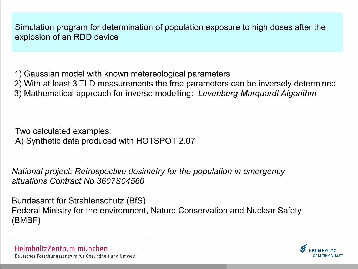
1) Gaussian model with known metereological parameters2) With at least 3 TLD measurements the free parameters can be inversely determined3) Mathematical approach for inverse modelling: Levenberg-Marquardt Algorithm

Two calculated examples:A) Synthetic data produced with HOTSPOT 2.07

National project: Retrospective dosimetry for the population in emergency situations Contract No 3607S04560

Bundesamt für Strahlenschutz (BfS) Federal Ministry for the environment, Nature Conservation and Nuclear Safety (BMBF)

Simulation program for determination of population exposure to high doses after the explosion of an RDD device

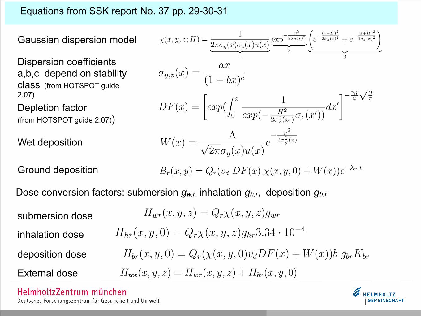
Gaussian dispersion model

• Atmospheric turbulence is also constant throughout the plume travel dis-tance.

• All of the the plume is conserved, meaning: no deposition or washout of theplume components; components reaching the ground are reflected back intothe plume; no components are absorbed by bodies of water or by vegetation;and components are not chemically transformed.

• Only vertical and crosswind dispersion occurs (i.e., no downwind dispersion).

• The dispersion pattern is probabilistic and can be described exactly by Gaus-sian distribution.

• The plume expands in a conical fashion as it travels downward, whereas theideal ”coning plume” is only one of many observed plume behaviors.

• Terrain conditions can be accomodated by using one set of dispersion coe!-cients for rural terrain and another set for urban terrain. The basic Gaussiandispersion equation is not intended to handle terrain regimes such as valleys,mountains or shorelines.

In short, the Gaussian models assume an ideal steady-state of constant mete-orological conditions over long distances, idealized plume geometry, uniform flatterrain, complete conservation of mass, and exact Gaussian distribution The dis-persion factor

!(x, y, z; H) =1

2"#y(x)#z(x)u(x)! "# $

1

exp! y2

2!y(x)2

! "# $2

%

e! (z!H)2

2!z(x)2 + e! (z+H)2

2!z(x)2

&

! "# $3

(1)

can be interpreted as the time integrated concentration of spread material by aunity source in [s/m3]. The coordinate system is Cartesian and depends on thelocation of the source and on its wind direction. The source is located in the originof the system at a given release height z above the surface. The positive x-axislies in the direction of the mean wind. The z-coordinate is the height above thesurface. The y-axis lies in the crosswind direction. The wind speed u (m/s) isaccounted in term 1; term 2 and 3 account the e"ective height H of the plumeand its width of the plume. In particular term 2 describes the crosswind shapeof the plume as a Gaussian curve with dispersion coe!cient #y peaked on the x-axis; Term 3 describes the reflecting e"ect of ground surface which adds a (z !Hcomponent to the z + H). Complete reflection is assumed.

2

Dose conversion factors: submersion gw,r, inhalation gh,r, deposition gb,r

1.1 Metereological parameters

The chi factor strongly depends on the height H of the release, the wind velocityand the dispersion coe!cients !y (m) and !z (m).

STACK HEIGHT : the actual plume height of the release may not be the phys-ical stack height. Plume rise can occur because of the velocity of stack emission,temperature di"erential between the stack area and the sorrounding air. There-fore, the rise of the plume results in an increase in the release height. E"ectiverelease height leads to lower integrated concentrations at ground level and it also’shifts’ the maximum concentration point of the plume towards higher x values.In this work, however, plume rise calculation is for sake of semplicity neglectedand the value for the e"ective height is left as input parameter H .

WIND VELOCITY:the wind velocity is measured at a given reference height href from the ground.The wind velocity profile is then given by

v(z) = v(href)(z

href)p (2)

where p depends on the stability class and is resumed in table ??

WIND DIRECTION:the wind direction is in metereology defined as the direction the wind comes from(e.g west wind is the wind coming from the west and flowing towards East). Whenthe direction is given in metereological degrees "met to work consistently in Carte-sian coordinates it is necessary to convert them into mathematical degrees withthe following equation

"math = "met + 180! (3)

In this work, input angle " for wind direction is the mathematical angle "math andit should be given in radians (rad = deg !

180).

DISPERSION COEFFICIENTS:The dispersion coe!cients are a function of atmospheric stability and depend onthe downwind distance x Their general form is:

!y,z(x) =ax

(1 + bx)c(4)

where x is the downwind distance in meters and a, b and c depend on the cloudcover and wind speed. They are taken from Briggs [?] combined with observa-tions out to downwind distance of 10 km. The set of equations used for !y,z are

3

Dispersion coefficients a,b,c depend on stability class (from HOTSPOT guide 2.07)

associated with dispersion experiments and are widely used (e.g they are also im-plemented in HOTSPOT Health physics code [?]). These formulas are applicablefrom a distance 0.1 km from the source to approximately 10 km.

Stability classes range from A to B where class A is the stability class thatdescribes the most stable weather condition and F is the most unstable one. In anunstable atmosphere there is more mixing and plumes are wider and higher thanin a stable atmosphere.

1.2 Dry deposition

The process of dry deposition accounts for aereosols depositing on surfaces as aresult of turbulent di!usion and browinian motion. Chemical reactions, impactionetc., combine to keep them at ground level. The e!ective deposition velocityvd [m/s] is empirically defined as the ratio of the observed deposition flux Fr

([Bq/m s]) and the observed air concentration Bq/m3 near the ground. As thismaterial is deposited on the ground, the plume above becomes depleted. Thedeposition velocity varies several orders of magnitude depending on the chemicalproperties of the source term. For most materials a reasonable value is 0.01 m/s.On the other hand, in this work, a value of 0.1 m/s is also used and will bediscussed in ??

The source term decreases with downwind distance. This is accomplished bymultiplying the original source term by the so-called depletion factor DF (x). Thedepletion factor DF (x) is given by

DF (x) =

!

exp(" x

0

1

exp(! H2

2!2z(x!)!z(x!))

dx!#" vd

u

"2!

(5)

1.3 Wet Deposition

In case of rain, deposition on the ground is also a function of rain intensity. Itis characterised by the scavanging e!ect of water droplets to the aereosols. Theso-called wash-out coe"cient W is given by

W (x) =#"

2"!y(x)u(x)e" y2

2"2y(x) (6)

with # = #0(II0

)0.8 where I is the measured rain intensity and I0 is the unit rainintensity [mm/h]. #0 = 7 # 10"5 s"1 is the wash-out coe"cient related to I0.

4

Depletion factor (from HOTSPOT guide 2.07))

2 Calculation of total dose

2.1 Ground deposition Br

Ground deposition [Bq/m2] is calculated from equation 1 and by considering bothdry deposition and wet deposition.

Br(x, y) = Qr(vd DF (x) !(x, y, 0) + W (x))e!!r t (7)

where "r is the decay constant ot the radionuclide r and t = x/u(x).

2.2 External gamma dose

The thermoluminescence dosimeters measure the total # dose Htot. This consistsof a submersion dose Hwr which is due to spread of radionuclides in the air and adeposition dose Hbr due to the emitted # radiation of radionuclides deposited onthe ground:

Htot(x, y, z) = Hwr(x, y, z) + Hbr(x, y, 0) (8)

To calculate a dosis to which a human being is being exposed, the so-called dosisconversion factors (DCF) are used. They link the #-dose rate [Gy/s] recorded bya detector to the surface contamination Bq/m2 or concentration on air Bq/m3.The absorbed dose rate Gy/s is converted into dose equivalent Sv/s by using aweighting factor 1 (average on whole body). Therefore, the units of DCF are Sv m3

Bq s

and Sv m2

Bq s for submersion dose gwr and deposited dose gbr respectively. Their valuesare tabulated in [?]. The submersion dose is then calculated as

Hwr(x, y, z) = Qr!(x, y, z)gwr (9)

whereas the deposition dose is calculated as

Hbr(x, y, 0) = Qr(!(x, y, 0)vdDF (x) + W (x))b gbrKbr (10)

where Kbr = 1!e!!r!t

!ris integration term, !t is the duration of exposure [s] and

b is 1 short after the rain. In this work, the TLD dosimeters are assume to beplaced at z = 1.

2.3 Internal gamma dose

Although TLD dosimeters measure only external exposure, for sake of complete-ness, also exposure due to inhalation is described. Dose to which human beingsare exposed via inhalation is calculated as:

Hhr(x, y, 0) = Qr!(x, y, z)ghr3.34 · 10!4 (11)

where ghr is the DCF for inhalation and 3.34 · 10!4 [m3/s] is the normal breatherate of an adult.

6

Ground deposition

2 Calculation of total dose

2.1 Ground deposition Br

Ground deposition [Bq/m2] is calculated from equation 1 and by considering bothdry deposition and wet deposition.

Br(x, y) = Qr(vd DF (x) !(x, y, 0) + W (x))e!!r t (7)

where "r is the decay constant ot the radionuclide r and t = x/u(x).

2.2 External gamma dose

The thermoluminescence dosimeters measure the total # dose Htot. This consistsof a submersion dose Hwr which is due to spread of radionuclides in the air and adeposition dose Hbr due to the emitted # radiation of radionuclides deposited onthe ground:

Htot(x, y, z) = Hwr(x, y, z) + Hbr(x, y, 0) (8)

To calculate a dosis to which a human being is being exposed, the so-called dosisconversion factors (DCF) are used. They link the #-dose rate [Gy/s] recorded bya detector to the surface contamination Bq/m2 or concentration on air Bq/m3.The absorbed dose rate Gy/s is converted into dose equivalent Sv/s by using aweighting factor 1 (average on whole body). Therefore, the units of DCF are Sv m3

Bq s

and Sv m2

Bq s for submersion dose gwr and deposited dose gbr respectively. Their valuesare tabulated in [?]. The submersion dose is then calculated as

Hwr(x, y, z) = Qr!(x, y, z)gwr (9)

whereas the deposition dose is calculated as

Hbr(x, y, 0) = Qr(!(x, y, 0)vdDF (x) + W (x))b gbrKbr (10)

where Kbr = 1!e!!r!t

!ris integration term, !t is the duration of exposure [s] and

b is 1 short after the rain. In this work, the TLD dosimeters are assume to beplaced at z = 1.

2.3 Internal gamma dose

Although TLD dosimeters measure only external exposure, for sake of complete-ness, also exposure due to inhalation is described. Dose to which human beingsare exposed via inhalation is calculated as:

Hhr(x, y, 0) = Qr!(x, y, z)ghr3.34 · 10!4 (11)

where ghr is the DCF for inhalation and 3.34 · 10!4 [m3/s] is the normal breatherate of an adult.

6

associated with dispersion experiments and are widely used (e.g they are also im-plemented in HOTSPOT Health physics code [?]). These formulas are applicablefrom a distance 0.1 km from the source to approximately 10 km.

Stability classes range from A to B where class A is the stability class thatdescribes the most stable weather condition and F is the most unstable one. In anunstable atmosphere there is more mixing and plumes are wider and higher thanin a stable atmosphere.

1.2 Dry deposition

The process of dry deposition accounts for aereosols depositing on surfaces as aresult of turbulent di!usion and browinian motion. Chemical reactions, impactionetc., combine to keep them at ground level. The e!ective deposition velocityvd [m/s] is empirically defined as the ratio of the observed deposition flux Fr

([Bq/m s]) and the observed air concentration Bq/m3 near the ground. As thismaterial is deposited on the ground, the plume above becomes depleted. Thedeposition velocity varies several orders of magnitude depending on the chemicalproperties of the source term. For most materials a reasonable value is 0.01 m/s.On the other hand, in this work, a value of 0.1 m/s is also used and will bediscussed in ??

The source term decreases with downwind distance. This is accomplished bymultiplying the original source term by the so-called depletion factor DF (x). Thedepletion factor DF (x) is given by

DF (x) =

!

exp(" x

0

1

exp(! H2

2!2z(x!)!z(x!))

dx!#" vd

u

"2!

(5)

1.3 Wet Deposition

In case of rain, deposition on the ground is also a function of rain intensity. Itis characterised by the scavanging e!ect of water droplets to the aereosols. Theso-called wash-out coe"cient W is given by

W (x) =#"

2"!y(x)u(x)e" y2

2"2y(x) (6)

with # = #0(II0

)0.8 where I is the measured rain intensity and I0 is the unit rainintensity [mm/h]. #0 = 7 # 10"5 s"1 is the wash-out coe"cient related to I0.

4

Wet deposition

Equations from SSK report No. 37 pp. 29-30-31

2 Calculation of total dose

2.1 Ground deposition Br

Ground deposition [Bq/m2] is calculated from equation 1 and by considering bothdry deposition and wet deposition.

Br(x, y) = Qr(vd DF (x) !(x, y, 0) + W (x))e!!r t (7)

where "r is the decay constant ot the radionuclide r and t = x/u(x).

2.2 External gamma dose

The thermoluminescence dosimeters measure the total # dose Htot. This consistsof a submersion dose Hwr which is due to spread of radionuclides in the air and adeposition dose Hbr due to the emitted # radiation of radionuclides deposited onthe ground:

Htot(x, y, z) = Hwr(x, y, z) + Hbr(x, y, 0) (8)

To calculate a dosis to which a human being is being exposed, the so-called dosisconversion factors (DCF) are used. They link the #-dose rate [Gy/s] recorded bya detector to the surface contamination Bq/m2 or concentration on air Bq/m3.The absorbed dose rate Gy/s is converted into dose equivalent Sv/s by using aweighting factor 1 (average on whole body). Therefore, the units of DCF are Sv m3

Bq s

and Sv m2

Bq s for submersion dose gwr and deposited dose gbr respectively. Their valuesare tabulated in [?]. The submersion dose is then calculated as

Hwr(x, y, z) = Qr!(x, y, z)gwr (9)

whereas the deposition dose is calculated as

Hbr(x, y, 0) = Qr(!(x, y, 0)vdDF (x) + W (x))b gbrKbr (10)

where Kbr = 1!e!!r!t

!ris integration term, !t is the duration of exposure [s] and

b is 1 short after the rain. In this work, the TLD dosimeters are assume to beplaced at z = 1.

2.3 Internal gamma dose

Although TLD dosimeters measure only external exposure, for sake of complete-ness, also exposure due to inhalation is described. Dose to which human beingsare exposed via inhalation is calculated as:

Hhr(x, y, 0) = Qr!(x, y, z)ghr3.34 · 10!4 (11)

where ghr is the DCF for inhalation and 3.34 · 10!4 [m3/s] is the normal breatherate of an adult.

6

2 Calculation of total dose

2.1 Ground deposition Br

Ground deposition [Bq/m2] is calculated from equation 1 and by considering bothdry deposition and wet deposition.

Br(x, y) = Qr(vd DF (x) !(x, y, 0) + W (x))e!!r t (7)

where "r is the decay constant ot the radionuclide r and t = x/u(x).

2.2 External gamma dose

The thermoluminescence dosimeters measure the total # dose Htot. This consistsof a submersion dose Hwr which is due to spread of radionuclides in the air and adeposition dose Hbr due to the emitted # radiation of radionuclides deposited onthe ground:

Htot(x, y, z) = Hwr(x, y, z) + Hbr(x, y, 0) (8)

To calculate a dosis to which a human being is being exposed, the so-called dosisconversion factors (DCF) are used. They link the #-dose rate [Gy/s] recorded bya detector to the surface contamination Bq/m2 or concentration on air Bq/m3.The absorbed dose rate Gy/s is converted into dose equivalent Sv/s by using aweighting factor 1 (average on whole body). Therefore, the units of DCF are Sv m3

Bq s

and Sv m2

Bq s for submersion dose gwr and deposited dose gbr respectively. Their valuesare tabulated in [?]. The submersion dose is then calculated as

Hwr(x, y, z) = Qr!(x, y, z)gwr (9)

whereas the deposition dose is calculated as

Hbr(x, y, 0) = Qr(!(x, y, 0)vdDF (x) + W (x))b gbrKbr (10)

where Kbr = 1!e!!r!t

!ris integration term, !t is the duration of exposure [s] and

b is 1 short after the rain. In this work, the TLD dosimeters are assume to beplaced at z = 1.

2.3 Internal gamma dose

Although TLD dosimeters measure only external exposure, for sake of complete-ness, also exposure due to inhalation is described. Dose to which human beingsare exposed via inhalation is calculated as:

Hhr(x, y, 0) = Qr!(x, y, z)ghr3.34 · 10!4 (11)

where ghr is the DCF for inhalation and 3.34 · 10!4 [m3/s] is the normal breatherate of an adult.

6

2 Calculation of total dose

2.1 Ground deposition Br

Ground deposition [Bq/m2] is calculated from equation 1 and by considering bothdry deposition and wet deposition.

Br(x, y) = Qr(vd DF (x) !(x, y, 0) + W (x))e!!r t (7)

where "r is the decay constant ot the radionuclide r and t = x/u(x).

2.2 External gamma dose

The thermoluminescence dosimeters measure the total # dose Htot. This consistsof a submersion dose Hwr which is due to spread of radionuclides in the air and adeposition dose Hbr due to the emitted # radiation of radionuclides deposited onthe ground:

Htot(x, y, z) = Hwr(x, y, z) + Hbr(x, y, 0) (8)

To calculate a dosis to which a human being is being exposed, the so-called dosisconversion factors (DCF) are used. They link the #-dose rate [Gy/s] recorded bya detector to the surface contamination Bq/m2 or concentration on air Bq/m3.The absorbed dose rate Gy/s is converted into dose equivalent Sv/s by using aweighting factor 1 (average on whole body). Therefore, the units of DCF are Sv m3

Bq s

and Sv m2

Bq s for submersion dose gwr and deposited dose gbr respectively. Their valuesare tabulated in [?]. The submersion dose is then calculated as

Hwr(x, y, z) = Qr!(x, y, z)gwr (9)

whereas the deposition dose is calculated as

Hbr(x, y, 0) = Qr(!(x, y, 0)vdDF (x) + W (x))b gbrKbr (10)

where Kbr = 1!e!!r!t

!ris integration term, !t is the duration of exposure [s] and

b is 1 short after the rain. In this work, the TLD dosimeters are assume to beplaced at z = 1.

2.3 Internal gamma dose

Although TLD dosimeters measure only external exposure, for sake of complete-ness, also exposure due to inhalation is described. Dose to which human beingsare exposed via inhalation is calculated as:

Hhr(x, y, 0) = Qr!(x, y, z)ghr3.34 · 10!4 (11)

where ghr is the DCF for inhalation and 3.34 · 10!4 [m3/s] is the normal breatherate of an adult.

6

submersion dose

inhalation dose

deposition dose

External dose

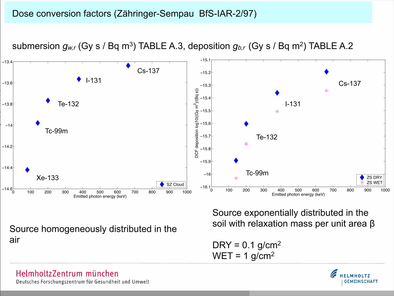
Dose conversion factors (Zähringer-Sempau BfS-IAR-2/97)

submersion gw,r (Gy s / Bq m3) TABLE A.3, deposition gb,r (Gy s / Bq m2) TABLE A.2

0 100 200 300 400 500 600 700 800 900 1000−14.6

−14.4

−14.2

−14

−13.8

−13.6

−13.4

Emitted photon energy (keV)

DC

F su

bmer

sion

log1

0((G

y m

3 )/(Bq

s))

SZ Cloud0 100 200 300 400 500 600 700 800 900 1000

−16.1

−16

−15.9

−15.8

−15.7

−15.6

−15.5

−15.4

−15.3

−15.2

−15.1

Emitted photon energy (keV)D

CF

depo

sitio

n lo

g10(

(Gy

m2 )/(

Bq s

))

ZS DRYZS WET

Xe-133

Tc-99m

Te-132

I-131Cs-137

Tc-99m

Te-132

I-131

Cs-137

Source exponentially distributed in the soil with relaxation mass per unit area β

DRY = 0.1 g/cm2

WET = 1 g/cm2

Source homogeneously distributed in the air

CODE: OPTLMDOSE.f90

MAIN PROGRAM SUBROUTINE FCN.f90 calculates objective function as log10(Dosedata) - log10(Dose)SUBROUTINE LMDIF from MINPACK runs optimisationSUBROUTINE COVAR calculates covariance matrix for error estimationcartesian axis: wind direction is x-axisINPUT datanamelist:&global_para rnuclide='Tc-99m' wind_ref=3.3d0 theta= 0.0d0 stability_class = 'A' H= 2.5d0 vd= 0.1d0 h_ref=2.0d0 dep_model=”DRY” I_rain = 0.0d0 eq_model=‘EXPONENTIALX’ xdata0=1.0d0 Dt_plot=60.0d0 Qr = 5.8D8/filename_read: x (km), y(km), Dose(Sv), Surface activity (kBq/m2), Dt(s)Radionuclide implemented are: Cs-137, I-131, Xe-133, Te-132, Tc-99mOUTPUT datafilename_save:info 1 M 23 N 1 opt_value 436806916.322 NORM 0.216464 unbiased sigmaX 9533334.244

+ other output files to produce plots

CODE: LEVENBERG-MARQUARDT ALGORITHM in MINPACK

F = log10(Dosedata)-log10(Dose)

For both cases, calculation with the logarithm is preferred due to the large rangingscales of value involved for both surface activity and dose values.

In general a non-linear square least problem is specified by a function F suchthat:

||F (xsol)|| ! ||F (x)|| (14)

where if the domain of definition of xsol is the entire domain of function F thenxsol is a global solution. If xsol is a solution of the nonlinear least square problem,then xsol solves the system of nonlinear equations

m!

i=1

fi(x)"fi(x) = 0 (15)

which in terms of Jacobian matrix implies the orthogonality condition:

F !(xsol)TF (xsol) = 0 (16)

Technically the algorithm determines a correction p to x that produces a su!cientdecrease in the residuals of F at the new point x+ p; it then replaces x with x+ pand begins an other iteration. The correction p depends upon a diagonal scalingmatrix D, a step bound " and an approximation J to the Jacobian matrix of FThe optimisation routine LMDIF from MINPACK delivers the optimised resultstogether with information whether optimisation has been succesfully completed ornot. In general, to understand whether the results of the optimisation are goodit is convenient first of all to compare visually the optimised function versus theexperimental one. In a second step it is useful to calculate the standard deviationfor the optimised value and to look at whether the squared-sum of the residuals hasdecreased towards zero during the optimisation steps. A plot of the residuals givesinformation about quality of optimisation. In addition, by using the covariancematrix, an estimate of the standard deviation of the obtained value can be given.

3.2 Convergence to a solution

The LMDIF routine [0] does various convergency tests between the approximationx and the solution xsol. Details related to these convergency tests are to be foundin the MINPACK manual. Here they are only briefly outlined:

• if the tolerance TOL is 10"K (usually set to machine precision) the finalresidual norm has K significant decimal digits then INFO is set to 1.

• D is a diagonal matrix whose entries contain scale factors for the variables.The larger component of D · x have K significant digits and INFO is set to2.

8

If xsol is a solution of a non-linear least square problem then x solves:

For both cases, calculation with the logarithm is preferred due to the large rangingscales of value involved for both surface activity and dose values.

In general a non-linear square least problem is specified by a function F suchthat:

||F (xsol)|| ! ||F (x)|| (14)

where if the domain of definition of xsol is the entire domain of function F thenxsol is a global solution. If xsol is a solution of the nonlinear least square problem,then xsol solves the system of nonlinear equations

m!

i=1

fi(x)"fi(x) = 0 (15)

which in terms of Jacobian matrix implies the orthogonality condition:

F !(xsol)TF (xsol) = 0 (16)

Technically the algorithm determines a correction p to x that produces a su!cientdecrease in the residuals of F at the new point x+ p; it then replaces x with x+ pand begins an other iteration. The correction p depends upon a diagonal scalingmatrix D, a step bound " and an approximation J to the Jacobian matrix of FThe optimisation routine LMDIF from MINPACK delivers the optimised resultstogether with information whether optimisation has been succesfully completed ornot. In general, to understand whether the results of the optimisation are goodit is convenient first of all to compare visually the optimised function versus theexperimental one. In a second step it is useful to calculate the standard deviationfor the optimised value and to look at whether the squared-sum of the residuals hasdecreased towards zero during the optimisation steps. A plot of the residuals givesinformation about quality of optimisation. In addition, by using the covariancematrix, an estimate of the standard deviation of the obtained value can be given.

3.2 Convergence to a solution

The LMDIF routine [0] does various convergency tests between the approximationx and the solution xsol. Details related to these convergency tests are to be foundin the MINPACK manual. Here they are only briefly outlined:

• if the tolerance TOL is 10"K (usually set to machine precision) the finalresidual norm has K significant decimal digits then INFO is set to 1.

• D is a diagonal matrix whose entries contain scale factors for the variables.The larger component of D · x have K significant digits and INFO is set to2.

8

and orthogonality condition is valid

LMDIF runs various convergency tests between approximation x and the solution xsol

INFO 1: if the final norm of the residual has K significant decimal digits compared to initial one (the assumed tolerance 10-K is set to square root of machine precision)

INFO 2: the larger components of (D‧x) have K significant digits compared to initial ones

INFO 3: if both 1 and 2 are fulfilled

INFO 4: if the norm of the residuals is orthogonal to the Jacobian matrix.This should be examined further: could be F(x)=0, some local minimum and accuracy is not implicit

The algorithm looks for a correction p such that F(x+p) ≼ F(x)To find appropriate p, the algorithm solves the problem: min{ ||f=J ‧p ||: ||D ‧ p|| ≼ Δ} where D is diagonal scaling matrix and Δ is a step bound

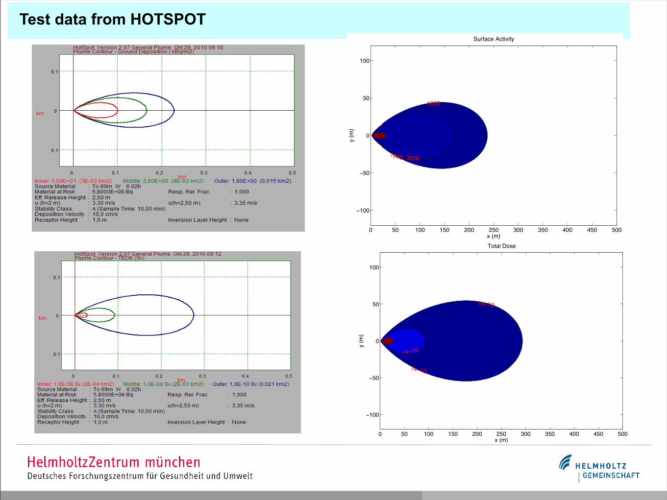
Test data from HOTSPOT

1800

1800 3500

Surface Activity

x (m)

y (m

)

0 50 100 150 200 250 300 350 400 450 500

−100

−50

0

50

100

1e−10

1e−10

1e−09

Total Dose

x (m)

y (m

)

0 50 100 150 200 250 300 350 400 450 500

−100

−50

0

50

100

Test data from HOTSPOT

- In principle with identical input values and initial guess, initial value for surface activity and dose should be the same as test data. BUT there is a difference of about 4-5% between the two

1 573338.11800501496 570000.00000000000 -3338.1180050149560 2 348971.81045471644 350000.00000000000 1028.1895452835597 3 123771.53738900440 130000.00000000000 6228.4626109956007 4 115940.33859631824 120000.00000000000 4059.6614036817627 5 65610.549861342719 68000.000000000000 2389.4501386572811 6 24991.867137796769 26000.000000000000 1008.1328622032306 7 20742.875084625062 21000.000000000000 257.12491537493770 8 9829.3327847436140 10000.0000000000000 170.66721525638604 9 6700.8849740578798 6900.0000000000000 199.11502594212016 10 4844.4895649776836 5000.0000000000000 155.51043502231641 11 4499.5026392314594 4700.0000000000000 200.49736076854060 12 2852.9649621150870 3000.0000000000000 147.03503788491298 13 2545.7964861216942 2600.0000000000000 54.203513878305785 14 2285.0045575781460 2400.0000000000000 114.99544242185402 15 2125.2379080010996 2200.0000000000000 74.762091998900360 16 2061.7740325329546 2100.0000000000000 38.225967467045393 17 1702.1308755155908 1800.0000000000000 97.869124484409213 18 1556.1511190830588 1600.0000000000000 43.848880916941198 19 1427.9172252346712 1500.0000000000000 72.082774765328850 20 1369.5773037010044 1400.0000000000000 30.422696298995561 21 1314.6877891197842 1400.0000000000000 85.312210880215844 22 1214.2254259686752 1300.0000000000000 85.774574031324846 23 1124.6957174068584 1200.0000000000000 75.304282593141579

- HOTSPOT CODE and OP_LM_BfS almost identical: the only difference is integration for Depletion factor!- In OPT_LM_BfS GAUSS integration is used to increase the number of steps during integration. HOSPOT uses trapezoidal rule but no possibility to check it

0 50 100 150 200 250 3000.65

0.7

0.75

0.8

0.85

0.9

0.95

1

x [m]

DEPL

ETIO

N FA

CTO

R

Test data from HOTSPOT: result

info 1 M 23 N 1 opt_value 436806916.322 NORM 0.216464 unbiased sigmaX 20804118.71 (sigmaX divided by M-N) convergence achieved after 9 iterations

50 100 150 200 250−10

−9.5

−9

−8.5

−8

−7.5

x log10(m)

Dose

log1

0(Sv

)

Exp DoseINI DoseOPT Dose

Test data from HOTSPOT: cloudshine and groundshine

1e−10

1e−10

1e−09

Dose cloudshine

x (m)

y (m

)

0 50 100 150 200 250 300 350 400 450 500

−100

−50

0

50

100

1e−10

Dose groundshine

x (m)

y (m

)

0 50 100 150 200 250 300 350 400 450 500

−100

−50

0

50

100

0 50 100 150 200 250 3008

8.5

9

9.5

10

10.5

11

11.5

12

12.5

x (m)

Gro

unds

hine

/Clo

udsh

ine

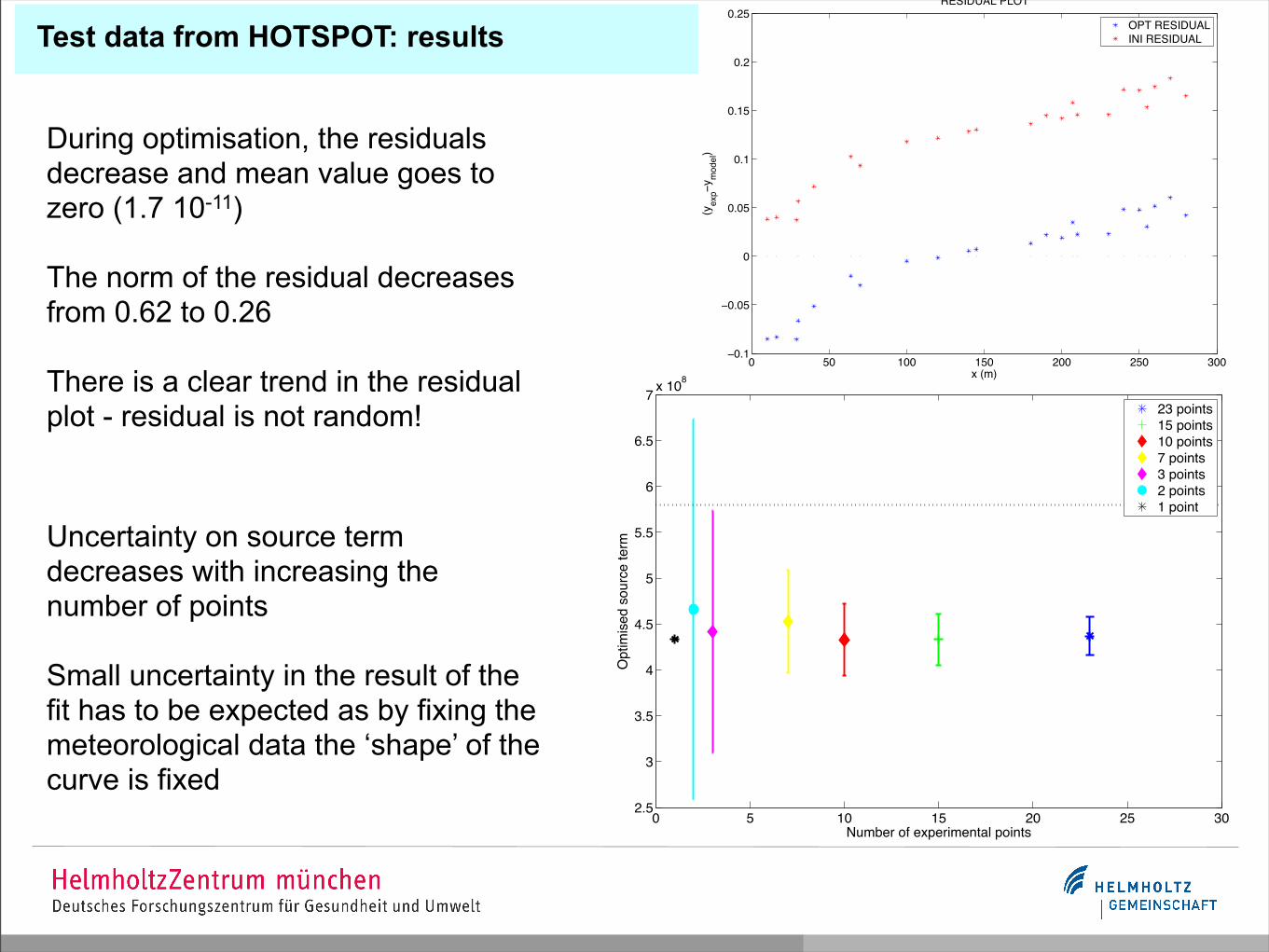
Test data from HOTSPOT: results

During optimisation, the residuals decrease and mean value goes to zero (1.7 10-11)

The norm of the residual decreases from 0.62 to 0.26

There is a clear trend in the residual plot - residual is not random!

Uncertainty on source term decreases with increasing the number of points

Small uncertainty in the result of the fit has to be expected as by fixing the meteorological data the ‘shape’ of the curve is fixed

0 5 10 15 20 25 302.5

3

3.5

4

4.5

5

5.5

6

6.5

7 x 108

Number of experimental points

Opt

imise

d so

urce

term

23 points15 points10 points7 points3 points2 points1 point

0 50 100 150 200 250 300−0.1

−0.05

0

0.05

0.1

0.15

0.2

0.25

x (m)

(yex

p−y m

odel

)

RESIDUAL PLOT

OPT RESIDUALINI RESIDUAL

Experimental data from Prouza et al.

TEST 2: 221 measurements of surface activity&global_para rnuclide='Tc-99m' wind_ref=1.10d0 theta= 0.00d0 stability_class ='B' H= 5.0d0 vd= 0.01 h_ref=2.0d0 I_rain = 0.0d0 Dt=45.0d0 Qr = 9.10D4/

- large uncertainty on deposition velocity vd- Initial source term (measured) is 910 MBq- Along x-direction, experimental profile of the plume is NOT an exponential - --> slow wind and clear Gaussian profile suggest diffusive process also in X direction: possibility for users to choose!- No source partitioning is included- objective function which is minimised is log10(Bdata+1) - log10(Br+1)

−10 0 10 20 30 40 500

20

40

60

80

100

120

140

160

180

x (m)

Surfa

ce a

ctiv

ity (B

q/m

2 )

ExperimentGauss fit

Fitted Gaussian profile x0=15 m, σx=5.13

( ) ( ) ( )220 2/ xxx óe=xdiffusivex −−

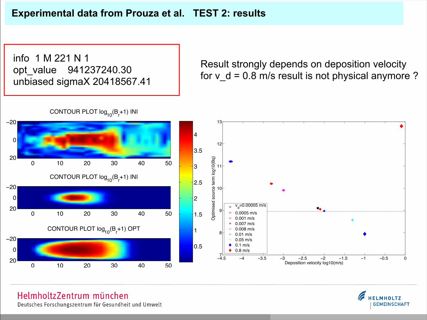
Experimental data from Prouza et al. TEST 2: results

info 1 M 221 N 1 opt_value 941237240.30unbiased sigmaX 20418567.41

0.5

1

1.5

2

2.5

3

3.5

4

CONTOUR PLOT log10(Br+1) INI

0 10 20 30 40 50

−20

0

20

CONTOUR PLOT log10(Br+1) INI

0 10 20 30 40 50

−200

20

CONTOUR PLOT log10(Br+1) OPT

0 10 20 30 40 50

−200

20 −4.5 −4 −3.5 −3 −2.5 −2 −1.5 −1 −0.5 07

8

9

10

11

12

13

Deposition velocity log10(m/s)

Opt

imise

d so

urce

term

log1

0(Bq

)

vd=0.00005 m/s0.0005 m/s0.001 m/s0.007 m/s0.008 m/s0.01 m/s0.05 m/s0.1 m/s0.8 m/s

Result strongly depends on deposition velocityfor v_d = 0.8 m/s result is not physical anymore ?

Experimental data from Prouza et al. TEST 2

0 10 20 30 40 50 60−6

−5

−4

−3

−2

−1

0

1

2

3

x (m)

RES

IDU

AL

INITIALFINAL

The norm of the residual decreases from 40 to 23

The residual clearly follows a trend and is not random but around zero

The standard deviation is very small....again by fixing meteorological data the form of the curve underlying the fit is fixed!

0 10 20 30 40 500

0.5

1

1.5

2

2.5

3

3.5

4

4.5

5

x (m)

Surfa

ce a

ctivi

ty lo

g 10(B

r + 1

)

−20 −10 0 10 200

0.5

1

1.5

2

2.5

3

3.5

4

4.5

5

y (m)

Surfa

ce a

ctivi

ty lo

g 10(B

r + 1

)

EXPERIMENTALINITIALOPTIMAL