comparing rainfall dependent inflow and infiltration ... · 1 comparing rainfall dependent inflow...

1

Comparing Rainfall Dependent Inflow and Infiltration Simulation Methods

leonard Wright, Shawn Dent, Charles Mosley, Paul Kadota and Yassine Djebbar

Rainfall dependent inflow and infiltration (RDII) is a significant, though undesirable, component of the m·ban wet-weather water budget in many sanitary sewer systems. Costs and environmental damage attributable to RDII are significant. Costs may be accrued tlu·ough increased treatment and conveyance cost-:, increased maintenance costs, and sanitary sewer overflows (SSOs ). To reduce these coste; and mitigate environmental damage, engineered solutions require estimations of the long-term characteristics of the RDII response to wet weather. This in turn requires estimation of the performance of the existing collection and treatment system, as well as the expected perfonnance of various possible solutions.

Due to the complex number of available pathways that RDII may enter a sanitary sewer, RDII is one of the most difficult components ofthe urban wetweather water budget to estimate. RDII observations typically indicate response times that may range from several minutes to several days or weeks. This is confounded by regional and/or seasonal groundwater trends that influence RDII response. Various tools have been applied to estimating this special hydrologic response, including the rational method and several unithydrograph methods. This chapter provides an overview of available RDII estimation methods and highlights results from arelativelynewphysically based conceptual method first introduced by Kadota and Djebbar ( 1998). Kadota and Djebbar (1998) reported on modifications to the USEPA SWMM RUNOFF model that include the response of a conceptual non-linear reservoir to changes in groundwater elevations resulting from permeable-area infiltration.

Wright, L.T., S. Dent, C. Mosley, P. Kadota andY. Djebbar. 2001. "Comparing Rainfall Dependent Inflow and Infiltration Simulation Methods." Journal of Water Management Modeling R207-16. doi: 10.14796/JWMM.R207-16. ©CHI 2001 www.chtjournal.org ISSN: 2292-6062 (Formerly in Models and applications to Urban Water Systems. ISBN: 0-9683681-4-X)

235

http://dx.doi.org/10.14796/JWMM.R207-16

236 Comparing RDII SImulation Methods

The model has recently been applied to a sanitary collection system in Vallejo California. Initial results indicate the modified RUNOFF model is very good at computing RDH, including the delayed, seasonally varying groundwater components of RDII. It is recommended that the USEPA SWMM model be updated with the revisions made by Kadota and Djebbar (1998).

16.1 Introduction

Excess wet weather flows in sanitary sewers may result in unacceptable public health risks and environmental damage. From an operational standpoint, problems associated with excess wet weather flows include excessive conveyance and treatment costs, decreased treatment efficiency and SSOs. SSOs have threatened public drinking supplies, contaminated residential areas \'lith raw sewage, and introduced pathogens, toxins and excess BOD loads to receiving waters (Golden 1996). Petroff (1996) estimates that nearly one-half ofthe treated wastewater in the United States comprises RDII and dry weather infiltration.

Estimation of the wet-weather response of a sanitary sewer system remains one ofthe more challenging problems encountered in urban hydrology. A "'ride variety of hydrologic methods have been proposed to accomplish this task, most of which are based on wen-established methods of surface runoff modeling. The rational method, unit hydrograph theOlY, and physically based conceptual methods have all been proposed. Crawford et a1. (1999), Bennett et al. (1999) and Dent et a1. (2000) present a review of these methods for RDII estimation. This chapter will also present an overview of these methods with some clarifications based on experience from a recent case study. In addition, a new method first proposed by Kadota and Djebbar (1998) will be presented. Preliminary results from a case study in Vallejo California using this method will also be presented. This method is a modification to the USEP A RlJNOFF block oftne Stonn Water Management Model (SWMM).

16.1.1 Definition of RDII

Rainfall derived inflow and infiltration is a complex component of the urban wet weather water budget as well as the sanitary sewer water budget. In general, RDU consists of inflow and infiltration. Inflow is storm water that enters sewers directly via manholes, directly connected drains (not always illegal or

16.1 Introduction 237

illicit) and cross-connected stonn sewers, among other possible direct or nearly direct pathways. These connections generally respond quickly to wet weather events. RDH also has a groundwater component known as infiltration. Infiltration may consist of nearly direct sources such as trench infiltration (TI) or infiltration from near-surface defects such as those associated with defects in the sewer latera1. TI results from infiltrated water that travels through the back-filled pipe trench, and enters through system defects such as loose pipe and manhole joint'S, cracks, etc. Infiltration also includes slow groundwater infiltration (GWI) sources.

Groundwater infiltration may consist of a component directly associated with rainfall events and a component associated with a wet season (i.e. impossible to isolate the response to one single rain event, but rather a mOlmding effect from a series of rain events plus a component resulting from regional groundwater flux). GWI may be characterized by a response on the order of days to months. Most difficulties associated with IllII estimation result from the complexities associated with the aWl response sih'11al.

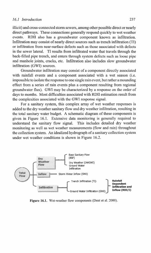
For a sanitary system, this complex array of wet weather responses is added to the dry weather sanitary flow and dry weather infiltration, resulting in the total sanitary water budget. A schematic diagram of these components is given in Figure 16.1. Extensive data monitoring is generally required to understand the sanitary flow signaL This includes detailed dry weather monitoring as well as wet weather measurements (flow and rain) throughout the collection system. An idealized hydrograph of a sanitary collection system under wet weather conditions is shown in Figure 16.2.

Base Sanitary Flow (BSF)

Dry Weather (DWGWI) Ground Water Infiltration

Storm Water Inflow (SWI)

Trench Infiltration (TI) } Rainfall Dependent Infiltration and

Ground Water Infiltration (GWI) Inflow (RDI/I)

.Figure 16.1. Wet-weather flow components (Dent et at 2000).


Month

.Figure 16.2. Idealized wet weather hydro graph for a sanitary collection system (Dent et al. 2000).

16.2 Review of Common RDII Estimation Methods

RDIT estimation methods are usually based on wen-established rainfall nmoff methods. These range from simple volmne fractions to physically based conceptuai models. This section provides an overview of the basis of these methods to provide a context for the research needs addTessed by Kadota and Djebbar (1998). In practice, any of these methods should be used with an accurate database of rain and flow observations during both wet and dry periods.

16.2.1 Rational Method Basis: the R Factor Method

The rational method has been used for over a century to estimate peak surface runoff rates for design purposes. The rational method simply uses a fraction of the rainfall rate to compute a nmoff flow rate. Commonly expressed as

16.2 Review of Common RDII Estimation Methods 239

Q=CiA, where Q is the runoff flow rate, C is the runoff coefficient, A is the contributing area and i is the rainfall intensity in units of rainfall depth/time. For RDII volume analysis, a similar assumption is made based on rainfall volume (i.e. the rate may be factored out of the rational method equation). Commonly known as the R-method, the ratio ofRDII volume divided by the rainfall volume is used to define R:

R = VRDIl

VR41N (16.1)

After R is fOlmd for a series of measured events, the calculated value may be used to estimate RDH volumes from other events. There is no standard method used to apply R to an "event", because an event may be defined in many ways. A peak R-value may be calculated for an individual storm event, while an average R-value can be calculated for a complex series of events (e.g. months of wet weather RDH). Reporting either of these two types ofR-values can be misleading if the duration of the event is not defined.

This method is generally too simple for design or permitting estimates because it does not take into account factors other than rainfall volume, e.g. seasonal changes, antecedent event conditions, or other time varying conditions that may affect RDIi response.

16.2.2 Unit Hydrograph Methods

The unit hydro graph (UII) is a linear model that can be used to transform measured rainfall into an estimated hydrograph (Chow et aI., 1988). The UR is based on the assumption that rainfall is constant in time and uniformly distributed over the catchment, and that the duration of runoff from a given depth of excess rainfall is constant (Chow et at, 1988). The principles oflinear superposition and proportionality are also assumed. The following three sections describe UH methods that may be used for RDII analysis:

1. a synthetic UR approach, where the shape of the hydro graph is first assumed,

2. the data-derived UIl, where the vector ofUH ordinates is derived directly :!}-om measured data using methods of unconstrained or constrained optimization, and

3. the Nash model, conceptualized as a series of linear reservoirs, along with recent work on the Nash model by Yue and Ilashino (2000).


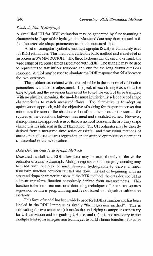
Synthetic Unit Hydrograph

A simplified UH for RDII estimation may be generated by first assuming a characteristic shape of the hydro graph. Measured data may then be used to fit the characteristic shape parameters to match measured data.

A set of triangular synthetic unit hydro graphs (SUB) is commonly used for RDII estimation. This method is called the RTK method and is included as an option in SWMM Ru"NOFF. The three hydrographs are used to estimate the wide range of response times associated with RDII. One triangle may be used to represent the fast inflow response and one for the long drawn out GWI response. A third may be used to simulate the RDII response that falls between the two extremes.

The problems associated with this method lie in thc number of calibration parameters available for adjustment. The peak of each triangle as well as the time to peak and the recession time must be found for each of three triangles. With no physical meaning, the modeler must heuristically select a set of shape characteristics to match measured flows. The alternative is to adopt an optimization approach, with the objective of solving for the parameter set that minimizes the sum of the absolute value of the deviations or the sum of the squares of the deviations between measured and simulated values. However, if an optimization approach is used there is no need to assume the arbitrary shape characteristics inherent in the RTK method. The VB ordinates may be directly derived from a measured time series or rainfall and flow using methods of unconstrained least squares regression or constrained optimization techniques as described in the next section.

Data Derived Unit IJ..vdrograph l"'v{ethods

Measured rainfall and RDII flow data may be used directly to derive the ordinates of a unit hydrograph. Multiple regression or linear programming may be used with complex or multiple-event hydrographs to derive a linear transform function between rainfall and flow. Instead of beginning with an assumed shape characteristic as with the R TK method, the data derived VB is a linear transform function completely derived from measurements. This function is derived from measured data using tec1miques oflinear least squares regression or linear programming and is not based on subjective calibration methods.

This form of model has been widely used for RDII estimation and has been labeled in the RDII literature as simply "the regression method". This is misleading for nvo reasons: (i) it masks the underlying assumptions necessary for UH derivation and for guiding UH use, and (ii) it is not necessary to use multiple least squares regression techniques to build a linear transform function


between rainfall and flow, when other and sometimes more appropriate methods exist. Since this method is easy to apply to measured time-series data commonly collected inRDII studies, it is importantto understand the limitations and flexibility of the UH.

Unit Hydrograph derivation using Least Squares Regression

For a single variable least-squares linear regression RDII estimation model, the dependent variable, y, is the volmne of RDII that flows past a basin metering point over a time interval. For the simplest case, the independent variable x is measured rainfall during that same intervaL

A limitation of this single variable model is that rainfaH has some basin response lag-time that may be viewed as travel time to the metering point and can be greater than a single time step. The volume of RDII that passes the metering point over a timestep may not originate completely from the rainfall that fell during that same timestep. There is a travel time to the metering point that is likely to be greater than the measurement time intervaL The RDII for observation i at time t is some unknown function ofthe antecedent precipitation, groundwater conditions, condition of the pipe network, geometry of the pipe network, etc. This logic leads to the development of a multiple linearregression model that uses the past rainfall to compute RDII.

The general regression model is expressed as (Neter et al. 1990):

Q/ :::: Po + PIPt .+- PZPt-l + P3Pt-Z + .... + PkPt-k+! (16.2)

for k independent variables, and t = 1,2, 3, ... n timesteps.

where: Qi computed RDH flow rate for observation i, P t recorded rainfall depth in inches during the tth hour,

f3 f3 regression intercept and coefficient, respectively. 0' II

Linear regression methods may be used to express a linear RDII response model based on the time series of recorded precipitation and flow. The estimated flow for each time step is a function of precipitation during the previous k time steps. The lagged rainfall variables may be adde{f to the model until the adjusted coefficient of multiple determination (R 2) reaches a maximum. The adjusted R2 should be used with multiple regression models to account for the degrees of freedom associated with multiple regression models. This multiple linearregression model may also be viewed as a unit hydrograph, where f3n in Equation 16.2 are the UH ordinates. Further details ofthe UH may be found in Chow et al. (1988), Dooge and Bruen (1989), Eagleson et aL (1966), Singh (1988), Bras (1990), and Bedient and Huber (1992).


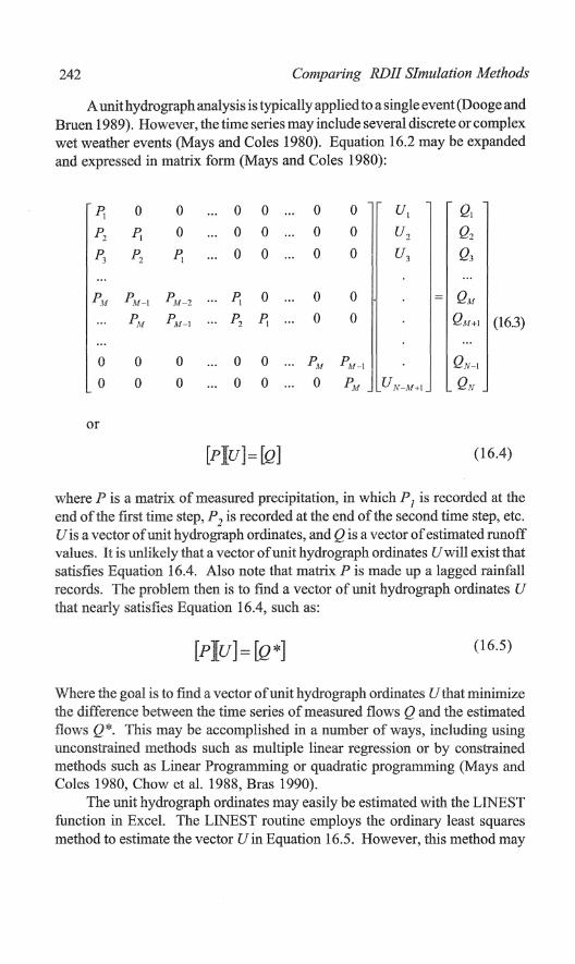
A unithydrograph analysis is typically applied to a single event (Dooge and Bruen 1989). However, the time series may include several discrete or complex wet weather events (Mays and Coles 1980). Equation 16.2 may be expanded and expressed in matrix form (Mays and Coles 1980):

~ 0 0 0 0 0 0 U1 QI P 2 ~ 0 0 0 0 0 U2 Q2

~ P 2 ~ 0 0 0 0 U3 Q3

!>,I{ !>,IH !>,1;-2 ~ 0 0 0 QM

!>'v PM-I Pz ~ 0

p:,j QM+I (16.3)

0 0 0 0 0 P,I/ QN-I

0 0 0 0 0 0 P,'f U N-M+I QN

or

[plu] = [Q] (16.4)

where P is a matrix of measured precipitation, in which PI is recorded at the end of the first time step, P 2 is recorded at the end of the second time step, etc. U is a vector of unit hydrograph ordinates, and Q is a vector of estimated runoff values. It is unlikely that a vector of unit hydrograph ordinates U will exist that satisfies Equation 16.4. Also note that matrix P is made up a lagged rainfall records. Thc problem then is to find a vector of unit hydro graph ordinates U that nearly satisfies Equation 16.4, such as:

(16.5)

Where the goal is to find a vector of unit hydrograph ordinates U that minimize the difference between the time series of measured flows Q and the estimated flows Q*. This may be accomplished in a number of ways, including using unconstrained methods such as multiple linear regression or by constrained methods such as Linear Programming or quadratic programming (Mays and Coles 1980, Chow et al. 1988, Bras 1990).

The unit hydro graph ordinates may easily be estimated with the LINEST function in Excel. The LINEST routine employs the ordinary least squares method to estimate the vector U in Equation 16.5. However, this method may


result in UH ordinates that are ill-behaved and physically unrealistic (Bras 1990). Negative values and total hydrograph volumes less than one along with oscillations in the hydro graph tail may result from using unconstrained regression methods (Bras 1990). Constrained methods such as linear programming (LP) as described below solve many of these problems.

Unit Hydrograph derivation using a Linear Program

The ordinary linear regression techniques described above use unconstrained least squares estimation techniques to fmd Q*. Bras (1990) argues that constrained methods offer several advantages over unconstrained regression techniques for UH ordinate estimation. Mays and Coles (1980) and Chow et aL (1988) describe UH ordinate estimation using LP, the most common constrained optimization formulation. There are two reasons why this method may be preferred over ordinary least squares regression:

1. Unconstrained re!:,'Tession methods are likely to result in several negative UH ordinates. Negative results may indicate multico linearity among variables (common in time series data (Bras and Rodrioguez-Iturbe 1993») as well as running counter to logic based on principles of mass balance (i.e. rainfall can not logically reduce downstream flow rate). On the other hand, LP methods are constrained to non-negative solutions, and therefore will result in positive UH ordinates (vector U* in Equation 16.5).

2. The objective of minimizing the squares of the residuals in not necessary in the LP formulation of the problem. The leastsquares objective has many computational benefits for analyses done without computers. However, there is little physical reason to weigh the outlier residuals so heavily against wen fitting values of estimated flow. In a linear program, an objective may be used to minimize the sum of the absolute value of the residuals.

The disadvantage for spreadsheet modelers is that two LP variables are required for each unknown element of U. While linear programs are relatively simple to formulate and solve in spreadsheets using the linear solver option, the size ofthe LP may quickly become unwieldy for a realistic number of time steps. This may necessitate the use of a more complex LP solver, as the standard Solver algorithm in Excel by Frontline Systems is limited to 200 variables. Mays and Coles (1980) and Chow et al. (1988) describe the details of the LP formulation used to solve for U in Equation 16.5 that minimizes the absolute difference between Q and Q*.

In summary, the RDII response models may be approached in several related ways. The first is a regression analysis on the time series of measured rainfall and flow. This results in a vector of regression coefficients f3 that may

244 Comparing RDll SImulation Methods

be applied to a rainfall record to generate a time series of estimated flow rates. The second way of approaching the linear RDII response model is with unit hydrograph theory. The unit hydro graph ordinates are estimated using an optimization technique such as ordinary least squares regression or LP. This results in a vector of unit hydro graph ordinates U* that may be applied to a rainfall record to generate an estimated time series of flow rates. The method refeHed to as "the regression method" in recent RDIT modeling literature is exactly equivalent to traditional unit hydrograph analysis.

Conceptually derived Unit Hydrographs

Unit hydro graph methods may also be derived using a system of cascading linear reservoirs. The theories behind the cascading reservoir models play an important conceptual link between purely empirical methods and more physically based conceptual models. The nonlinear reservoir used in SWMM runoff is related to these models, though more commonly derived via more physically based methods using continuity and momentum principles.

Singh (1988) and Bras (1990) describe the cascading linear reservoir method of deriving an instantaneous UH as fIrst proposed by Nash (1957). The original UH proposed by Shennan in 1932 may be derived as a special case of one linear reservoir with one outlet (Yue and Hashino 2000). Nash (1957) proposed using multiple linear reservoirs in series. As with the data-derived UH described above, the reservoir characteristic parameters may be found using an optimization scheme such as linear least squares regression or linear programming. Like the data-derived UR, the reservoir parameters may be constrained to physically realistic values with an LP, while with ordinary regression methods the parameters may be physically unrealistic (i.e. negative UH ordinates). This may be important if the goal is to develop a conceptual model based on physical parameters of the system.

The reservoir parameters are not necessarily physically based, even if the logic used to construct the system confIguration is based on physical propelties of the system. For example, Yue and Hashino (2000) use a system ofthree linear reservoirs and one parallel reservoir to simulate both fast and slow runoff components. This method has implications for RDH estimation because the slo\v response of OWl is often difficult to simulate, just as the interflow components of streamflmv as addressed by Yue and Hashino (2000). An LP was used to estimate the characteristics of the four reservoirs in the system to match a measured time series off1ow rates for a catchment in Japan (Yue and Rashino 2000).

16.3 Modifications to SWMM RUNOFF ... 245

16.3 Modifications to SWMM RUNOFF by Kadota and Ojebbar (1998)

The sun and data-derived un methods described in section 16.2 are empirical methods based on observations of rainfall and flow. There are three strong arguments against the use of these methods for RDII estimation:

1. The physical processes of surface runoff are knmvn to be nonlinear and dependent on antecedent watershed conditions. The processes of RDII generation are more complex than surface runoff alone.

2. It is difficult to simulate the delayed influence of GWl on RDII response purely from rainfall observations because the rainfall signal is greatly dampened.

3. The rational method and un methods described above are based on measurements of rain and flow. If modeled conditions do not match the conditions of the measurement, model results could be in en·or. In general, physical process information is important for analysis beyond the range of system observations.

These concerns suggest a model based on knowledge of the physical nature of the system. A logical step would be to link rainfall and groundwater infiltration based on knowledge ofthe processes of the urban water budget. A fraction of rainfall that infiltrates into pervious urban areas becomes GWl in the sanitary collection system. This process information may be used in a mechanistic manner and integrated into familiar physically-based conceptual models like SWMM. Recent work in Canada and Califomia indicate that this approach has great potential in improving GWl estimation.

A physically-based conceptual model also has the potential to be used to estimate the reduction in RDII from collection system rehabilitation. This method employs multiple hydro graphs that characterize the separate components of a wet weather hydrograph (DWF, rainfall dependent inflow and infiltration, and GWI). This method also applies an effective-area parameter that is common to each ofthe wet weather related hydrographs. Therefore, a reduction in the effective area parameter could be made based on the amount of rehabilitation work completed in a basin. This reduction could be applied in the model to obtain a hydrograph that would be representative of the wet weather response of the system after rehabilitation methods are applied. This area reduction has a variable effect on the hydrograph, as opposed to a constant reduction factor that would be applied in non physically-based methods.


Kadota and Djebbar (1998) describe recent modifications made to the SWMM RUNOFF block for the Greater Vancouver Regional District using this idea. In addition to the RTK method described above, SWMM RUNOFF has the ability to simulate GWI using a simple groundwater head estimation equation. Unfortunately, this method was not adequate to simulate measured G\lJ1 rates in Vancouver. Kadota and Djebbar (1998) made two important observations regarding flow processes in sanitary sewers:

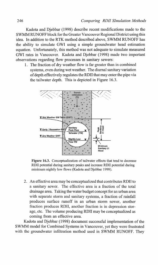
1. The fraction of dry weather flow is far greater than in combined systems, even during wet weather. The diurnal sanitary variation of depth effectively regulates the RDU that may enter the pipe via the tailwater depth. This is depicted in Figure 16.3.

M~nimum SanfiaryUi H_

:Figure Hi.3. Conceptualization of tailwater effects that tend to decrease RDU potential during sanitary peaks and increase RDII potential during minimum nightly low flows (Kadota and Djebbar 1998).

2. An effective area may be conceptualized that contributes RDII to a sanitary sewer. The effective area is a fraction of the total drainage area. Taking the water budget concept for an urban area with separate storm and sanitary systems, a fraction of rainfall produces surface 11.moff in an urban stOlID sewer, another fraction produces RDll, another ii'action is in depression storage, etc. The volume producing RDII may be conceptualized as coming from an effective area.

Kadota and Djebbar (1998) document successful implementation of the SWMM model for Combined Systems in Vancouver, yet they were frustrated with the groundwater infiltration method used in SWMM RUNOFF. They

16.3 Modifications to SWMM RUNOFF ... 247

proposed modifYing the groundwater flow model in SWMM based on wellfounded knowledge of the physical processes of RDII and the wet weather water budget. SWMM RUNOFF uses a conceptual nonlinear reservoir to generate flow.

16.3.1 Modifications Made to SWMM RUNOFF to Estimate RDII

The governing equation for RDII generation from groundwater in the CUlTent official version ofS\VMM RUNOFF is (Kadota and Djebbar 1998):

GWI = a j (Ecw -- E PI)D.. - a2 (En!' - E PI )b2 + a3 (Eow )(ET)y,·) (16.6)

where: GJf7

Eew EPI

E TW

al' a2, a3, bI, b2

the ground water infiltration flow, elevation of the groundwater table, pipe invert elevation, elevation of the tail water, and discharge coefficients.

Kadota and Djebbar (1998) note that Equation 16.6 does not take into account the driving head of the groundwater, the difference between the groundwater table and the tailwater elevation as shown in Figure 16.3, namely (EevIEm..). A revised equation may be written that replaces the pipe invert elevation with the tailwater elevation in the first parentheses (Kadota and Djebbar 1998):

GWI = a1 (Eow - Erw)b1 - a2 (Env - E PI )1>2 + a3 (EGW )(Erw)

(16.7) This subtle change creates the potential for the elevation of dry weather

flow in the pipe to affect the rate of infilh'ation entering the pipe. Without this driving head, infiltration would not occur. Equation 16.7 represents the behavior of a reservoir, the physical dimension of which is defmed by the effective RDH contributing area, the depth of pipe, and soil properties (Kadota and Djebbar 1998). Inflow to the reservoir is defined by percolating surface water, and the release rate of the reservoir is defined by the groundwater equation and its discharge coefficients (Kadota and Djebbar 1998).

For the modeler, the use of Equation 16.7 over the empirical methods described in section 16.2 is important. The physical characteristics of the system are explicitly defined with the conceptual model; therefore some ancillary Imowledge may be brought into the analysis. Though empirical methods may match measured data as well or better than conceptual models,


the conceptual model contains infonnation regarding the physical system, and may therefore be a more reliable tool for design analysis. This physical basis of the model becomes important when pipeline and manhole rehabilitation are investigated using the model. RDII reductions due to upgrades within the basin can be more accurately estimated when the variables producing the hydrographs can be adjusted to reflect the estimated reduction in influent flows (e.g. effective area). The next section compares results given by the modified SWMM model and a simple UH derived from multiple regression methods.

16.4 Case Study: Vallejo Sanitation District

Recent work for the Vallejo Sanitation and Flood Control District (VSFCD) in Northern California demonstrates the need for process modeling when planning for SSO remediation measures. Three RDII estimation methods were calibrated from measured rainfall and collection system flow data:

1. data-derived UR using linear regression in Excel, 2. data-derived UB based on an LP using Excel Solver, and 3. the modified SWMM RUNOFF code.

All three methods were used to simulateRDII response from basin VAOI in the VSFCD, a basin characterized by a large amount of GWI. The sewers in this basin are usually below groundwater most of the year. This basin has 168,000 lineal feet (51,000 m) of sewer, ranging from 6 inches to 27 inches (152-686 Imn) in diameter, upstream of the meter location. This equates to approximately 9% of the system (based on lineal footage of sewer). It comprises mainly residentiallanduse with some commercial activity. Most of this basin is also VCIY close to the Napa River.

16.4.1 Unit Hydrograph Method using the LlNEST Function in Excel

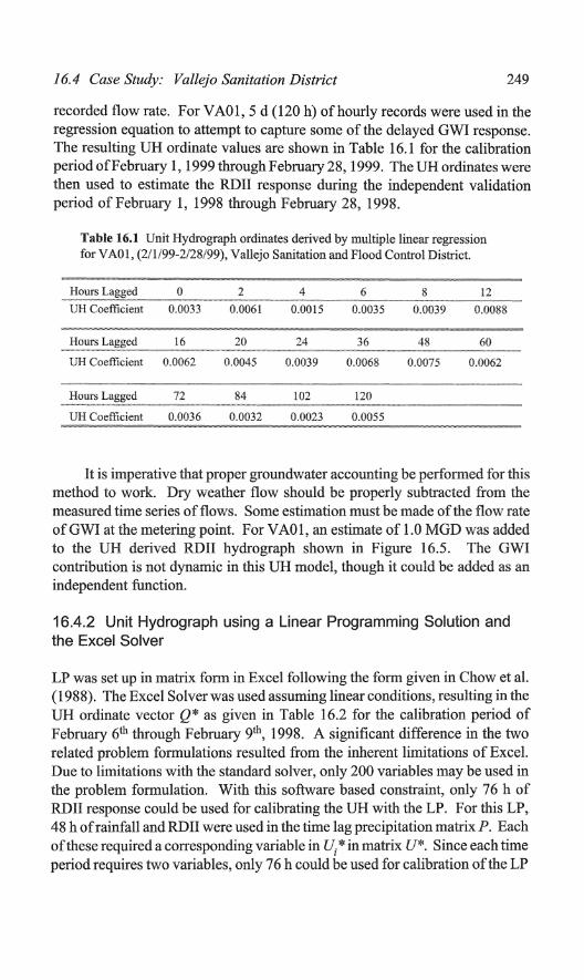
One of the easiest methods for deriving UH ordinates from measured time series data may be perforn1ed in a standard spreadsheet. The LINEST function was used in ~ficrosoft Excel to develop a multiple linear regression model as described in section 16.2.2. The rainfall record was lagged in time and the matrix P in Equation 16.3 was constructed. A limitation in Excel prevents more than 16 explanatory variables to be used in LINEST. Since the time series of rainfall and flow were recorded in hourly intervals, and the RDII response exceeded 16 hours, an averaging scheme ,vas developed. Averages of up to 18 h were used to develop a multiple linear regression model that used a total time lag of 120 h. This is shown in Table 16.1, where the 16th explanatory variable is the average rainfall that feU between 102 and 120 h prior to the

16.4 Case Study: Vallejo Sanitation District 249

recorded flow rate. For VAOl, 5 d (120 h) of hourly records were used in the regression equation to attempt to capture some of the delayed GWI response. The resulting UH ordinate values are shown in Table 16.1 for the calibration period ofF ebruary 1, 1999 through February 28, 1999. The UH ordinates were then used to estimate the RDII response during the independent validation period of February 1, 1998 through February 28, 1998.

Table 16.1 Unit Hydrograph ordinates derived by multiple linear regression for V AO 1, (211/99-2/28/99), Vallejo Sanitation and Flood Control District.

__ "-",,~~'>.%~~,,==-,~~:o,~·0W<:,,.:"'m .. ,,>:" __ ~~"V -Hours 0 2 4 6 8 12

lJH Coefficient 0.0033 0.0061 0.0015 0.0035 0.0039 0.0088

~'" ""="_. -" -Hours 16 20 24 36 48 60

(JH Coefficient 0.0062 0.0045 0.0039 0.0068 0.0075 OJ)062

Hours 72 84 102 120

UH Coefficient 0.0036 0.0032 0.0023

It is imperative that proper groundwater accomlting be performed for this method to work. Dry weather flow should be properly subtracted from the measured time series of flows. Some estimation must be made of the flovi; rate ofGWI at the metering point. For VAOl, an estimate of 1.0 MGD was added to the UH derived RDII hydrograph shown in Figure 16.5. The GWI contribution is not dynamic in this DR model, though it could be added as an independent function.

16.4.2 Unit Hydrograph using a Linear Programming Solution and the Excel Solver

LP was set up in matrix form in Excel following the form given in Chow et al. (1988). The Excel Solver was used assuming linear conditions, resulting in the DR ordinate vector Q* as given in Table 16.2 for the calibration period of February 6th through February 9th, 1998. A si!:,l11ificant difference in the two related problem formulations resulted from the inherent limitations of Excel. Due to limitations with the standard solver, only 200 variables may be used in the problem formulation. With this software based constraint, only 76 h of RDU response could be used for calibrating the UH with the LP. For this LP, 48 h of rainfall and RDII were used in the time lag precipitation matrixP. Each of these required a corresponding variable in Uj * in matrix U*. Since each time period requires two variables, only 76 h could be used for calibration of the LP


(48 UH ordinates + (76 h x 2 variables/h) = 200 linear LP variables). This is a limitation to solving the UH ordinates on a standard spreadsheet, however other software packages are available to solve LPs with a greater number of variables.

Table 16.2. LP derived unit hydrograph ordinates.

_____ =_._,'~_.~ .. ~.==.%=.~ ______ ill •• ==~." ••. ".= ... = .. =.=="~.~_ ... =_~~. ==~_ ~.H!§.J""'!£'~m~m..,.Q"~.~ ....... J. .......... _ .. m_.1, .••• ~~3~ ... _ .. ~4.. ... _ .......... Lm._ ...... =.Ji ................... l ..... _.=.

UH Coeff. 0.0085 0.0044 0 0 0 0.0036 0 0.0002

::::ifuI\l~!;.<L .. : ... ~ ...... ~~ .... =::2::=~ __ N~~ ... ::.: .. Li.:.::·:'j£:::=~===il.= ..... ::_~14 15 UH Coeff. 0.0023 0.0()3] 0.004 0.0034 0.0014 0.00]9 0.0041 0.0018

""""" :l ~ ""'"_ ~.- =" "'.-~ ""' •

.. =H!]..J·aggedm~_~= .... .l2m ...... lj_~= .... n.=m=_-1ll,.~ ...... _49~.=~_ .. JQ .... ~~_ .. UH Coeff. (l0026 0.0012 0 0 0 0 0.00] 0.0011 ~~_~~ _____ ... _._= .. ~.. ill ill_" = ....... ~_ •• == ••• __ ...... __ • ______ _

_ HlliJ.c!!gg"g •• "=_ ••• IL ..... _ ... _ .. ";?} ....•..........• "2;L~_35 ... _.m ..... J,L .. "_ ....... _.dL"~"._lL~ ..... J2~ ..... UH Coer!: 0.0024 0.0025 0.0004 0.0002 0.002 0.0019 0 0

Due to the linear solver limitations in Excel, only the regression based UH results are plotted in Figures 16.4, 16.5 and 16.6.

16.4.3 ROil Response using SWMM RUNOFF Version 4.31d

The modified version of SWMM RUNOFF as described in section 16.3 was used to simulate the entire wet weather sanitary water budget. This is compared to the DH methods, where independent estimates of OWl were needed to match measured flows. The modified RUNOFF performed very wen over a range of calibration periods. This model was also used for many other basins in the area with widely varying GWI responses. The ability to simulate the effect of the ground\vater driving head on the diurnal flow pattem of the total sanitary flow was also critical. The amount ofRDII is a flmction of the time of day due to standard diumal flow pattems. This was effectively simulated using this version of SWMM.

The use of a process-modeling environment is very important in an engineering design context. The ability to link other useful and trusted routing schemes in SWMM to the RUNOFF derived hydro graphs is invaluable to extrapolate to continuous time series analysis for design problems. For example, as shown in Figure 16.4, the RUNOFF generated RDII portion of the


... t ..

MODIFIED SWIIIIIIII RUNOFF

NOT OVER PREOICTiiD (VERlfEJ UPSTREAM SSOs)

REGRESSION BASED UNIT HYOROGRAPH

251

0,5 1;

0.25 I C

'.. ._... ..........••... - ...... ~,. @_5 ~

....

2JliOO

_RA.INFALL . . MF:I"sURED RDII RESPONSE

l .1

-MODELED Roa RESPO~"SE

025 .g x

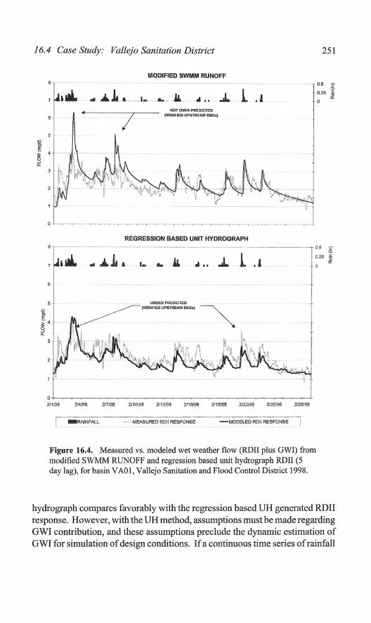
Figure 16.4. Measured vs. modeled wet weather flow (RDIl plus GWI) from modified SWMM RUNOFF and regression based unit hydro graph RDII (5 day lag), for basin V AO 1, Vallejo Sanitation and Flood Control Distlict 1998.

hydTograph compares favorably with the regression based UH generated RDII response. However, with the UH method, assumptions must be made regarding GWI contribution, and these assumptions preclude the dynamic estimation of GWI for simulation of design conditions. If a continuous time series of rainfall

252 Comparing RDII SImulation Afethods

is used to simulate the RDH response for design-based frequency analysis, the modeler must make assumptions regarding the potential GWl contributions during the entire time series (typically covering many years of rainfall records). This is an extremely tenuous assumption for the designer, as the GWI may be a function of the season, the condition of the stormwater drainage system, the regional groundv.mter conditions, and other aspects of the physical system. While the modified SWMM RUNOFF RDII model also has limitations in these areas, the process sinmlation enviromnent allows the modeler some basis for making judgments regarding the driving head of grOlmdwater over the sanitary collection system for continuous simulation.

Another major difference between the SWMM methods and the UH methods is in the method of calibration. For UH methods there are optimization schemes readily available to derive ordinates directly from the calibration data; there is no need for manual calibration adjustment. The calibration problem for physically based models is more problematic. The parameters fall conceptually between values that can be directly measured and those that have little or no physical meaning. For example, the reservoir capacity has a relationship to the size of the contributing RDII area, however this is a somewhat ambiguous value. SWMM calibration is typically done manually, without the aid of an optimization or search algorithm. For this reason, the distinction between "calibration" and "validation" becomes somewhat blun'ed for the practicing engineer. To create the best model possible, all available data are typically used to adjust model parameters. Generally flow and rain observations are very expensive to collect, and there are rarely enough good data to leave out of the calibration process to create a hue validation pedod. The S~'MM results presented here are no different. The 1998 wet season was the year ofEl Nino in California, and these valuable data were used in the calibration process. Therefore, the SWMM hydrograph presented in Figure 16.4 made use of the 1998 rainfall information, while the regression based UH model did not.

The hydrographs shown in Figure 16.4 demonstrate the ability of the modified R1JNOFF calculations to simulate the delayed aWl response. Constant G\Vl flows can be added to the UH RDII response to match calibration periods, but the static nature of this method is questionable for long term simulation analyses done to support design decision making. The dynamic nature of the physically-based conceptual model proposed by Kadota and Djebbar (1998) appears to warrant further attention from the SWMM community for RDH analyses. The hydro graph recession period shows the sensitivity of the groundwater elevation to wet and dry periods.

The total simulated hydro graph is shown in Figure 16.5, which comprises dry weather flow (from dry weather measurements made in August), the rapid RDII contribution (inflow and trench infiltration), and the delayed aWl


'0

E S 9 u.

I ••

4

2

MODIFIED SWMM RUNOFF

.. .. NOT OVER PREDiCTED

(VERIFIED UPSTREAM SSOS)

l .A

1 ~

REGRESSION BASED UNIT HYDROGRAPH 8

l .,

2/1/93 2i7/$9

IiIiIIIRIIlNFN.L MEASURED TOTAL RES-"ONSE -MODELED TOTAL RESPONSE

Figure 16.5. Measured VS. modeled total flow from modified SWMM RUNOFF and regression based unit hydrograph RDIT (5 day lag), for basin VAOI, Vallejo Sanitation and Flood Control District 1998.

253

0_5

0.25 j~

i ~

0.5 ~

f:25 1

component. For many design based analyses, continuous simulation is required to estimate the long term failure frequencies of SSO controls (i.e. SSOs occurring on average no more frequently than once every five years). The ability to simulate the antecedent groundwater conditions before each RDII event is critical to the success of this type of analyses. This process model


appears more appropriate for continuous simulation than empirical methods, which require static assumptions regarding GWI. Work currently underway indicates this method is appropriate for long-term continuous simulation. Figure 16.6 illustrates the component flows used to create the total modeled hydro graphs.

MODIFIED SWMM RUNOFF ST····

1 .4

REGRESSION BASED UNIT HYDROGRAPH

2J1/HH 2/4198 2i7/9a 2110mB 211319£ 2j16/fJB 21H119B 2/Z7iM 2/25198 2123198

Figure 16.6. Modeled component hydrographs for SWMM RUNOFF and regression based unit hydrograph RDH (5 day lag), for basin V AOI, Vallejo Sanitation and Flood Control District 1998.

0.5 I (i,25 g 0 ~

16.5 Conclusions 255

16.5 Conclusions

This chapter described some commonly used hydrologic methods for estimating RDII hydrographs. A recently proposed nonlinear reservoir process-based model was also described and compared using measured data from a sanitary system in Vallejo CA. Based on results from this case study, the following conclusions were made:

1. Physically based process models are better suited to design because processes may be more effectively simulated than with methods based purely on limited observations. Also ancillary physical infomlation such as flow routing may be important to the engineering solution. Empirical methods rooted in unit hydrograph theory may provide very good calibration results, but are less descriptive of the system under consideration.

2. Physically based models may better represent groundwater infiltration, an especially difficult element of the urban wet weather water budget to simulate. An empirical model would need to encompass vast amounts of seasonal time series data to capture the long-tenn groundwater fluxes into a collection system. A process model such as proposed by Kadota and Djebbar (1998) captures important elements of the physical process with relatively little infonnation.

3. The assumptions that must be made regarding the long-tenn GWl contribution to RDII response severely limit empirically based methods (e.g. regression and unit hydro graph methods). Process modeling of the driving groundwater head frees the modeler from making unsubstantiated assumptions regarding GWl contribution.

4. A process simulation environment that includes flow routing is an important tool for extrapolating from a relatively small calibration period to an extended time series of rainfall from which design events are commonly estimated.

5. Based on these limited results, the work of Kadota and Djebbar (1998) should be included in further SWMM research and development. In keeping with the overall SWMM philosophy, reducing the empiricism in system modeling tools by increasing the physical knowledge of the system will increase the utility of these tools for engineering design applications.

6. Application of the modified SWMM allows for more accurate calibration to the total flow hydro graph. This is possible because the three component flow hydro graphs are output (DWF, RDII, and GWl).

256 Comparing RDII Simulation Methods

7. The use of a physically-based conceptual model can more accurately estimate the reduction of RDII than other empirical methods. The SWMM model's effective area coefficient can be reduced to estimate a variable amount ofRDII and GWI reduced from a basin at each time step. Constant reduction in RDII is typically used for empirical models. The use of constant (or nearly constant) reductions in GWI will under or over estimate the amount of total flow during a continuous simulation modeling effort.

References

Bedient, P.B., and Huber, W.C. (1992). Hydrology and Floodplain Analysis, 2nd Edition. Addison-Wesley, Reading, MA.

Bennett, D. Rowe, R., Strum, Wood, D., Shultz, N., Roach, K., Spence, M., and Adderley, V. (1999). Using flow prediction technologies to control sanitary sewer overflows. 97-CTS-8. Water Environment Research Foundation, Alexandria, VA.

Bras, R.L. (1990). Hydrology, An Introduction to Hydrologic Science. AddisonWelsey Publishing Company, Reading, MA.

Bras, R.L. and Rodriguez-Iturbe, L (1993). Random Functions and Hydrology. Dover Publications, New York, 1-.rY.

Chow, V.T., Maidement, D.R. and Mays, L.W. (1988). Applied Hydrology. McGrawHill, Inc., New York. NY.

Crawford, D., P.L. Eckley and E. Pier. 1999. "Methods for Estimating Inflow and Infiltration into Sanitary Sewers." Journal of Water Management Modeling R204-17. doi: 10.14796/JWMM.R204-17.

Dent, S., Wright, L., Mosley, C., and Housen, V. (2000). Continuous simulation vs. design storms comparison with wet weather flow prediction methods. WEF Collection Systems Specialty Conference 2000. Rochester, NY.

Dooge, J. and Bruen, M. (1989) Unit hydrograph stability and linear Algebra. J. of Hydrology, 1 I 1. pp. 377-390.

Eagleson, P.S., Mejie-R, R. and March, F. {1966). Computation of optimum realizable unit hydrographs. Water Resources Research, Vol. 2, No.4, pp. 755-764.

Golden, J.B. (1996). An introduction to sanitary sewer overflows. In USEPA National Conference on Sanitary Sewer Overflows (SSOs) EPA/625/R-96/007. Office of Water, Washington, DC.

Kadota, P ., and Djebbar, Y. (1998). Simulating infiltration and inflow in sewer systems using SWMM RUNOFF. In WEF. Advances in Urban Wet Weather Pollution Reduction, Alexandria, VA.

Mays, L.W., and Coles, L. (1980). Optimization of unit hydrograph determination. Journal of the Hydraulics Division, VoL 106, HYl, 85-97.

Nash, J.E. (1957). The form of the instantaneous unit hydrograph. International

http://dx.doi.org/10.14796/JWMM.R204-17

References 257

Association of Scientific Hydrology Publication 45(3). Pp. 114-12l. Neter, J., Wasserman, W. and Kutner, M.H. (1990) Applied Linear Statistical Models,

Regression, Analysis of Variance and Experimental Design, third edition. Irwin, Homewood, IL.

Petroff, R.G. (1996). An Analysis of the Root Causes ofSSOs. In USEPA. National Conference on Sanitary Sewer Overflows (SSOs) EPA/625/R-96/007. Office of Water, Washington, DC.

Singh, v.P. (1988) Hydrologic Systems: Vol. 1, Rainfall-Runoff Modeling. PrenticeHall, Englewood Cliffs, NJ.

Yue, S. and Hashino, M. (2000). Unit hydrographs to model quick and slow runoff components of streamflow. Journal of Hydrology, 227, p. 195-206.

comparing rainfall dependent inflow and infiltration ... · 1 comparing rainfall dependent inflow...

Documents