CHAPTER17

Methods for Estimating Inflow and Infiltration into Sanitary Sewers

David Crawford, Paul Eckley and Edwin Pier

Excessive inflow and infiltration during wet weather periods into capacity­constrained sewer systems cause sanitary sewer overflows (SSOs). The two major components of wet weather flow are inflow and infiltration, and arc the main factors found in sanitary sewer evaluation studies (SSES) or inflow/ infiltration (III) studies. Control and reduction of inflow and infiltration directly relates to effective controls for SSOs.

The interaction and relative proportions of inflow and infiltration determine the extent, effectiveness and cost of control measures. Usually, control of direct inflow is the first source pursued, with the infiltration component either lumped into part of the inflow as an immediate response, or neglected because of the dominance of peak flow rates induced by inflow. The peak flow rate, as compared to sustained elevated flows from infiltration, is usually the sought-after result in SSES or III studies. Successful and accurate estimates of both rainfall-derived inflow and sustained flmvs from rainfall-derived infiltration are therefore the prime determinants ofthe effectiveness and cost of the controls.

The objective of this chapter is to summarize and provide some critique of C01l\i1\0\'\ 't'\0\V -pm)ect\on met\1odo\ogies, \)articu\arly methods that\)red\ct rainfall­derived inflo~v and infiltration or rainfall-derived inflow/ infiltration (RDH). A summary ofthe most common methodologies is included. Space limitation precludes site by site comparisons of each technique, even if project objectives (and funding) allowed such comparisons to be made.

Crawford, D., P.L. Eckley and E. Pier. 1999. "Methods for Estimating Inflow and Infiltration into Sanitary Sewers." Journal of Water Management Modeling R204-17. doi: I 0.14796/JWMM.R204-17. ©CHI 1999 www.chijournal.org ISSN: 2292-6062 (Formerly in New Applications in Modeling Urban Water Systems. ISBN: 0-9697422-9-0)

299

300 Estimating Inflow and Infiltration into Sanitary Sewers

The chapter will include discussion ofthe approach used in two communi­ties, one of medium size (population 160,000) and one large (800,000). Both communities have examples of varied infrastructure age and conditions, and climatic differences that affect inflow or infiltration prediction. The two commu­ni.ties have large capital improvement programs that are signit1cantly impacted by the quality and accuracy of flow estimates of design stonn flows. Design flows are estimated for current flow conditions as well as for future basin conditions with growth projections and infrastructure improvements. Infrastructure im­provements in general and specific to Salem, Oregon and Honolulu, Hawaii are to reduce inflow and infiltration, normal lite cycle system maintenance, or to enlarge sewer system capacity.

17.1 Sanitary Sewer Flow Components

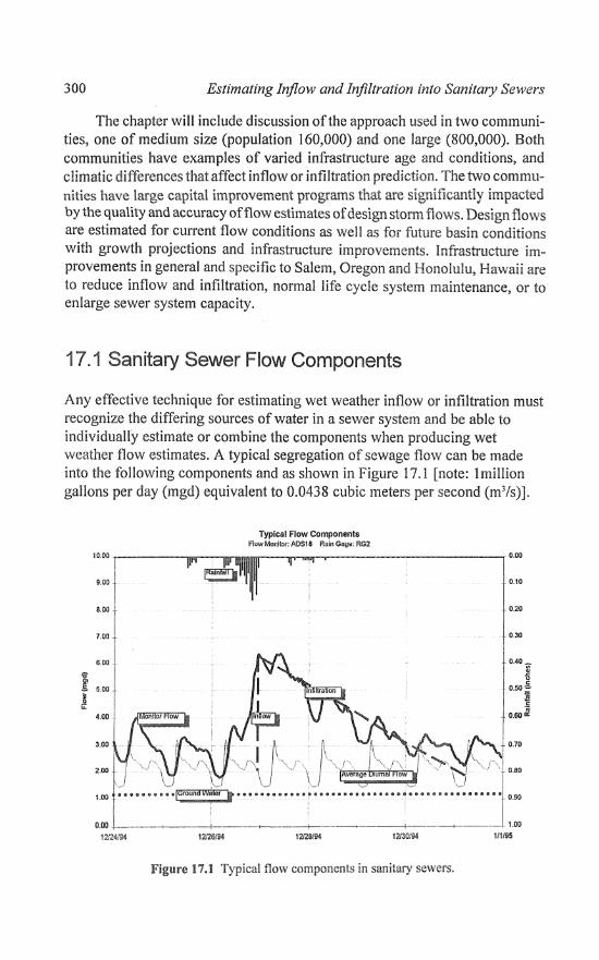
Any effective technique for estimating wet weather inflow or infiltration must recognize the differing sources of water in a se\ver system and be able to individually estimate or combine the components when producing wet weather flow estimates. A typical segregation of sewage flow can be made into the following components and as shown in Figure 17.1 [note: 1 million gallons per day (mgd) equivalent to 0.0438 cubic meters per second (m3/s)].

I ~ .9 ..

Typical Flow Component. Flow Manitor. ADS18 Rajn Gage: 002

10.00

9.00

8.00

7.00

6.00

5.00

4.00

3.03

2.00

1.00

. ______ ~ 0.00

I t 0.10

1020

I t 0.30

0.40_

~ O.50~

~ ·i

0.60 '"

0.70

0.80

0.00 .\ __________ +-__ . -.---+----- -.;.------.. ------+----- _____ + _______ , ... ___ ._ ... _._-"" 1.00

12'24~'94 111195

Figure 11.1 Typicai flow components in sanitary sewers.

172

(ADF): Base th)m community's domestic, commercial and industrial customers, the everyday sewerage generated by the community. This flow usually has a diumal with a normal peak occurring in the morning wake-up time, sometimes another peak occurs in the afternoon and a low flow during the night and early morning hours. Industrial and

commercial components would follow workday patterns. The difference between the monitor flow and ADF at the start of Figure 17.1 is due to residua! infiltration from previous rainfall. Groundvi/ater: Sewer flow usually associated with seasonal changes in base infiltration to the system but not as a result of immediate wet periods. long cyclic change in ground water levels due to seasonal rainfall patterns has the greatest influence on ground water flow. Pipe condition and relative elevation between the pipes and ground water level also affect ground water flow.

• Inflow: Usually an immediate and noticeable rise in sewer flow as a direct response to rainfall. There is usually a short time Jag between time of rainfall and observed sharp rise in flow response. Inflow is dependent upon antecedent conditions, the condition of the sewer system particularly lateral connections and the number of direct hydraulic connections.

o Infiltration: Response to rainfall. Typically a slower response to rainfall that can build with time as rainfall continues and may last for several days after rainfall stops. Infiltration is dependent upon antecedent conditions, pipe conditions and soil characteristics.

301

Common methods for estimating the components of sewer system flow usually perform the following determinations and consider the various effects mentioned above:

• Determinations of dry weather flow and ground water infiltration. • Detennination of flow rates for inflow and infiltration.

Determination of hydrograph shape or constant peak rates. Inclusion of effects of antecedent conditions. Evaluation of possible changes to inflow and infiltration compo­nents due to remediation projects.

17.2 Evaluation of Flow Methodologies

Many methods have been used to develop flow estimates into sewer systems. It is common to develop extensive data and processes to estimate dry weather flows and diumal patterns and only cursory data and single value estimates of wet weather 11ow. Data on basin areas, and population are collected and to accurate estimates of daily

302 Estimating Inflow and Infiltration into Sanitary Sewers

flow rates. Diurnal patterns or daily peaking factors are also developed and applied to dry weather flow to produce a peak dry weather flow rate. On top of this flow is usually applied a constant peak wet weather flow reiated to a basin's size, total population or population equivalent. The relative levels of effort expended if! developing dry weather flows versus \-vet flows are often in reverse tlYotlorti.on to tne 'PeaK fiow genemteu b'j t\\e t\\lCl c\m\\1\me\\\~.1'n\'b !,)n.~\\ results in conservative peak flow rates, uncertainty or total 110ws and greatly affects the sizing of sewers and SSO control Obviously it is more difficult to develop wet weather flows that are a result of spatial and time varying rainfall over the sewered basin. The following therefore provides a summary of common methods for estimating wet weather flow in sewerage systems.

17.2.1 Constant Unit Rate

Components ofRDU can be estimated as a constant unit rate based on se\vered basin (sewershed) characteristics. Unit rates are dependent on many variables and often vary significantly from sewershed to sewershed. Most communities however have peak inflow infiltration rates incorporated design manuals. The design manual specifies the unit flow rate, usually as a rate per acre, !()r new or existing development. Some common assumptions for constant rates are the projection of peak f10w rates recorded at the wastewater treatment plant to other parts of the system based on basin area or length and diameter in the basin.

RDn from large areas should be based on independent variables such as sewershed area (gallons per acre), land use (gallons per acre of specific land use), population (gallons per capita), and pipe length (gallons per foot of pipe). Small areas can be fUI1her refined such that the independent variables include charac­teristics related to system defects (leaky manholes, poor pipe conditions, etc.) and to other characteristics such as pipe material and age, roof drain connections, back-fill material, and construction practices.

17.2.2 Percentage of Rainfall Volume (R-Value)

The ratio, in percent, between the volume of wet weather flow at a monitoring location and the rainfall volume that falls on the sewershed area served by the monitor is defined as the R-value. To compute the R-value, average base flow and ground water flow components are first determined by analyzing metered data for extended dry periods. Wet-weather RDU is then detennined by subtrac:ting the average base flow and ground water components from metered data for typical

duration wet periods. The volume ofRDH for significant (typically events with greater one inch - 25 mm - is data and divided the rainfall volume to storm.s.

I? 2 E .. 'aluation lvfethodologies 303

Additional analysis is usually carried out to determine approximate hydrograph shape for the time increment ofthe rainfall or design storm selected. A triangular hydrograph shape is typically used. The hydro graph shape deter­mines the time to peak inflow and the time for flows to recede or the recession of flow atter rainfall ends. Each time period triangular hydrograph is superim­posed with the other hydrographs to produce the design storm hydrograph for the

total storm event duration. Under ideal conditions the R-values would measure the response of the

sewershed to rainfall events and are therefore dependent upon antecedent conditions. Both the amounts of inflow and infiltration will be affected by the condition of antecedent soil moisture. Rainfall variation across the basin and unceliainties in measuring flow and rain are two examples that make conditions Jess than ideal. The assumption of dry weather and ground water flows can also greatly affect estimation of the R-value. Figure 17.2 shows a series of storm events. Often seasonal envelope curves are developed to represent wet or dry antecedent conditions. Figure 17.2 illustrates wet and dry envelope curves drawn to enclose the high and low extremes.

For design purposes an upper bound or envelope curve for R-value is determined based on a plot of all recorded or selected R-values. The rainfall design storm volume and duration is determined from rainfall frequency analysis. The corresponding design storm flow volume is selected from the upper bound R-value for the design rainfall amount. The design storm volume is combined with the assumed hydrograph shape to determine the wet weather inflow

·l

I .. - -"- ! !IJiYCoMihon EnvelfJPel3~ l ) ·-----11 ..

.. ; .. . I

1--. __ ._._. __ .. __ • ______ --..... -,----- ---------~-------_---.--.- ---___ - _......J 2.5 3

Rainfall + Snowmelt Volume {lncMs}

Figure 17.2 'R' Factor determination.

304 Estimating Inflow and Infiltration into Sanitary Sewers

hydrograph for that point in the system. The total hydrograph is the sum of the wet weather hydrograph, the usually assumed constant ground water flow and the diurnal dry weather flow.

17.2.3 Predictive Equations Based on Rainfall and Flow Regression

The rainfall and flow multiple regression method uses observed rainfall and flow to derive a relationship between rainfall and ROIL This relationship is then used to estimate ROn flows for other rainfall periods of interest or for a design stann with given volume and duration. Because rainfall response will vary with antecedent conditions, it is necessary to develop separate equations to represent summer and winter conditions. The equations can be adjusted to fit both the inflow peak and recession limbs ofthe sewer flow hydrograph. The general form of the equation relates time period rainfall to the wet weather response, such a..<;:

where:

wet weather response in cfs or mgd series of coefficients produced from regression analy­sis, and rainfall values corresponding to the time periods se­lected during the regression analysis.

A graph showing the 'creation' oftheregression equations is given in Figure 17.3. Figure 17.3 shows the diurnal pattern and daily flow pattern. This pattern

oftlow is selected from monitor data (during dry weather) and applied consis­tently across the time period. The wet weather flow is added to the assumed dry weather flow for each time step (usually one hour) to reconstitute the total wet weather flow at the monitor site. The regression equation is given at the bottom of Figure 17.3 and shows the coefficients and time intervals used to determine the rainfall to wet weather response relationship. For this monitor location, time intervals ranging from 1 hour to 168 hours have been used with 360 hours not used (hence the zero coefficient). The process developed to create the relationw

ships can be easily modified to change the time intervals or drop time periods from the regression. Good data is obviously a prerequisite for a successful regression.

Figure 17.4 shows the extension of the regression analysis to other time periods. Average dry weather flow pattern is again assumed to be consistent

across the time period with wet weather response estimated from rainfall data applied through the regression equation for the monitor site (Cra\vford Engineer-

Associates, 1997).

r • (£

'6" '" .§. ~

~

ft~i~§~~ Equ~w.:m C$~~1't

flow M""iIQr. AOB1S Rain Gogo: RG2

-'!f'"""""-"---'

fU!O

7,00

6.00

5.00

4.00

2.00

.-----r Q,OO

I f 0,10

10,20 I 10.30 I I

30S

-1 0.40 _ I •

i ~ .l 0,50'§' I :i!

"I 060~ ........ -I 0,70

"',1 t 0.30

::::L-----~- --+--~ .... ---+-------~----!---.. ---__ J: 12124194 12f.ZBJ94 12Jl(Y94

Equatiun: RDB n O,SO", hi' -} 2.03"'3 hJ' -+ 4.74"0 hr ... 2.73*12 hr + 3.10"24 hr ~ 1.7$·48 hr -+ O.82*9G hr + O.13~166 hr + 0.00"360 ht

Figure 17.3 Regression tlow compared to monitored flow.

Regression Equmion Calibration fiow Monitor: AOS18 Rain Gage: RG2

':: rl-r~'l1nr'IT--'-' -- ----, -'f l"' 8001

7.0G -~

6.00

5,00

4.00

300

;t~:C

1.00 ~

111195

0.00

_j_ O.lO

OAO .. ~

0.50 :? J! ,~

0.60 It:

0.70

0.90

0.00 i--.. ~""- .• -"-----""---~--~--~------'''''-'''---'--~----~-----' _______ • ____ • ___ .~ ___ ~ __ ~.l,DO

12/10104 12iHiS4 12/24.'94 12/31/94

EqtltMlOrr RDU '" ::1.90·1 hr + 2.U3<3 hr + 4.74·6 hr + 2.73"12 hr -+ 3.10*24 hr + 1.76~4S hr ... O.fi2~!#"0 hr + 0.13·168 rof 1- O,()OV36Q hr

Figure 17.4 Application of rainfall- wet weather flow to other time periods.

306 Estimating Inflow and Infiltration into Sanitary Se'wers

The uncertainty in applying a point rainfall record to an area and the accuracy of the monitor data all tend to cause the engineer to select the time periods that produce the' best fit' curve to the observed data. I n other words visual judgements rather that rigorous statistical application are applied. The shOlter duration time intervals of the regression help the model express the amount of immediate inflow whHe the \ongerti.mcs heir) model the inf\\ttatkm that can occur when rainfall stops. The former selected to match peak flows and the latter the recession of flow. Other examples of regression applications in waste\vater analysis can be found in Berthouex and Box (1996).

17.2.4 Other techniques

Obviously there are many other methods and techniques available to produce reliable and appropriate wet weather flow hydrographs. Several other techniques are summarized below. The nature of the study area and the objectives of the study should be considered in applying approximate or other methods, particu­larly methods that are not verified against sewer flow measurements.

@ Percentage a/Streamflow: 'Streamflow can be a reliable predictor of RDII because the combinations of hydrologic conditions that increase streamflow are similar to those that impact RDH entering a sewer system. A relationship is developed between sewer flow monitoring data and streamflow data. The relationship is used to provide flow estimates in non-monitored basins but with adjacent streamflow data. In applying this relationship it is assumed that the sewer system conditions where the relationship is being applied are consistent with conditions in the monitored sewershed areas.

@ Unit Hydrograph: Unit hydrograph theory can be applied to sewer system monitor data just as in other hydrologic analysis. The unit hydrograph method assumes that RDII responds to rainfall volume and duration in the same manner as stormwater runoff and that the shape of an RDH hydro graph is a function of basin characteristics. Basic assumptions of the method are: that the time duration ofRDH hydrographs attributable to rainfall of a specific duration are con­stant and the peak flow is proportional to the volume of rainfall. Based on these assumptions, unit hydro graphs for RDII can be developed and calibrated against monitoring data. Several unit hydrographs may be necessary to represent the separate compo­nents contributing to the RDII hydrograph (inflow and infiltration) and adequateJy represent the hydrograph shape. The resulting unit

hydrograph can be scaled in proportion to a rainfall of desired intensity and duration to produce an RDH response hydrograph.

17.3 Techniques used in Salem and City and County (?lHonoiulu 307

\I Probabilistic: The probabilistic method is a frequency analysis peak ROIl flows and is similar to classical hydrologic frequency analysis for extreme events such as floods or peak rainfall events. The method can be applied to either sewer flow rates or event volumes. To apply the method, the peak value (rate or volume) is identified for each month in a period of record that covers a

representative period of wet and dry seasons. A statistical analysis is performed to determine recurrence intervals for each of these flows. The peak flows are ranked and plotted on log-probability paper. Values for various recurrence intervals can be determined fi'om the graph. Unlike some other methods that strive to derive RDn as some function of rainfall, the product of a probabilistic analysis is a relationship of sewer flow to recurrence interval. Greaterdiscussion ofthis (and the many other techniques mentioned herein) would violate the space allotment for this chapter.

17.2.5 ROll as a part of Commercial Hydraulic Software

There are numerous hydrology/hydraulics software packages that are widely used in the industry. These include XPSWMM, Mouse, Hydro Works and Hydra. All ofthe packages include methods (with various levels of detail and sophisti­cation) for generating dry weather flows and wet weather inflow and infiltration. Detailed review oftne methods ofthe commercial packages is beyond the scope of this chapter. In most cases the packages rely on standard rainfall runoff principles that consider hydraulically connected area, infiltration and ground water to sewer flow interactions to produce wet weather !low. Dry weather flows are estimated through assumptions on unit flow rates and population estimated and equivalents. Most also allow import of externally determined flows. Input of externally generated flows to hydraulic model systems is a common practice in SSO and SSES studies. Combined sewer overflow studies usually include watershed evaluation to determine stomlwater runoff (such as with the S\VMM RUNOFF block). In many cases one ofthe techniques outlined above is used to input the contribution fi'om sanitary or separated areas that contribute flow to a combined sewer system.

17.3 Techniques used Honolulu

Salem and City and County of

The discussion of the techniques and some of the observation of use and results obtained from applying the flow estimates to the two systems can only provide a cursory overview and some salient observations. Much work has been

308 i!.stimating h?flow and If?iiltration into Sanitary Servers

performed in collecting and analyzing data, evaluating alternative flow method­ologies, and assessing the flow-related impacts to the two collection systems of the City of Salem, Oregon (Salem) and the City and County of Honolulu, Hawaii (CCH). Salem has a current population of about 160,000 and CCH serves a total population 1,000,000. The intent ofthe sttldies should be considered when applying ~md aS~essing appropriate now estimation methods. No single method is perfect; if the flo\,1 methodology is selected with the objectives ofthe study clearly in mind and the degree of conservatism inherent in the method understood then results produced will usually be acceptable. The discussion given below is not a critique of the work performed by the many people and companies that have been involved with the various studies.

The studies for Salem and CCH contain many common elements. These include:

Recognition of the need to monitor datu throughout the system. The monitor data consists of both permanent monitor locations, for long term evaiuation of the collection system performance and tempo­rary gages that are used to determine and isolate basin t1mvs. The latter gages move around the system to 'find' the leakiest sub-basins and to assess the success of remediation projects. Flows throughout the systems can be extreme. Some basins have peak wet weather flow to average day flow ratios of 10 - 15. Many basins however have ratios in the expected range 00 to 6. Soil type, hydrology, system condition, construction practice and age of pipe are factors determining the wet weather response of the systems. Even in the relative small area of Salem there are observable differences between sewered basins that can be factored by some physical parameter such as age of pipe. In CCH the rainfall patterns playa substantial role in determining flow rates in the many basins ofihe collection system. Both systems are subject to surcharging and flooding or overflows. The regulatory pressures to eliminate, control and reduce overflows are high in both communities for many reasons. Each system has as a starting point a standard storm to control. In Salem the 1 in 5-year, 24-hour stOlW during winter months is the controlling event. In CCH a range of events from 1 in 2-yearto 1 in 1 O-year 6 hour storms are being considered.

For Salem extensive use of the regression method was used to estimate flows from basins to the collection system. The flow estimates were used as input to a detailed hydraulic model of the system. More details can be found in the

reports and appendices of the SSES study and Master Plan (CH2M Hill, 1994, 1996).

17.3 Techniques used in Salem and City and County of Honolulu 309

In CCH the primary studies are for sewer rehabilitation and III minimization (CCH, Fukunaga and Associates, I 994a and b, 1997). The' R' F actor method was used in CCH with dry weather flows computed using the WIMS (Wastewater Information Management System) (CH2M Hill, 1995). The effect of the flows to the collection system was simulated using a hydraulic model developed from data contained in WIMS.

17.3.1 Selecteci observations anci use of the flow methodologies

Estimation offutureflows from existing and new development A significant concern in many SSO and SSES studies is the estimation offuture conditions. Pr~iection of population growth and definitions of urban growth boundaries often provide the framework for determining future base and peak wet weather flow rates. Base flow rates can be obtained from overlay of traffic analysis zone data or other basin data with sewershed areas in elaborate GIS systems (see Crawford and Limtiaco, 1996). Often estimates offuture peak flow fi'om newly developed or developing areas rely on a simple assumption of a constant unit flow tied to estimated area or population. In Salem, an approach was adopted to refine these future rates, based upon observed monitor data and projected rates for the 5-year 24-hour storm event using the regression equation developed for the monitor locations.

Figure 17.5 shows the relationship found between the peak rate per acre for the 5-year storm and the average age of pipe in the basin. The variation in unit flow rate with age is apparent. This relationship quickly dispersed the idea of using a single unit flow rate for new areas, future basins that would develop in the next ten years but would be 20 years old at the 30 year planning horizon, or basins that have population growth but no increase in area. Based on the t1ndings of this analysis, Salem adopted 1,SOO gallons/acre/day (glald) for 10 year old basins, 3,OOOgiaid for 20 year old basins and 6,OOOg/aid for 30 year old basins. This approach allowed for the expected deterioration of the collection system as basins aged and provided a better tool to plan new sewers and expansions to treatment facilities and pump stations (CH2M Hill, 1994, 1996). Many basins hovvcver had reductions in basin flow rates due to rehabilitation projects.

The regression approach also provided a means of determining hydrograph sha\1e far future basins. the wet weather flow for new basins were based upon the hydrographs and !lxmd from monitor data newer basins of the existing collection system. Adjustments to flow rates were scaled using basin area.

Regression analysis limitations A major drawback of the regression approach is the adequate representation of the seasonal rainfall-inflow/infiltration process in a sanitary sewer system. Adequate and representative rainfall and flow data are pre-requisite for this

310 Estimating hiflow and Irifiltration into Sanitary Sewers

Peak Houri). RDIl r'le"w iWle p-•. .'r B.lsIn CompJred to t:i!) of Sui em ASSI.Il-llcJ Vatut;S

5 YCJ:lf DCS~ilfi Storm Fmm KCl!(c;;-~ion Efitwtlu;:!;

9,{l{JU r--'~-'-------------------'.-'-----'-".""""""-""-"---"' ...... _ .. _-_ . ..,

1,UOO

6,noo

5,H!¥J

4,{)W]

3,000.

2,iWO

II WYcl}rOId B;!sm

1,000 .. W .. !uCreek

10 15

.CwkCrxk

ill 2:t: Y CM Old BMta

• Brush Cdkgc W.

20 25

.. FoiJI~1~if:t;?{('b Imj

Figure 17.5 Estimation of unit flow rates and average pipe age in a basin.

30,00 ,...--___ ...

i I i

25,00 T

i

20.00 r

Ragreuion Equation CaJibr .. tion Flow Monitor: ADS18 Rain Gage: RG2

!f---rrlll"~-1 :: ... .,. Monjtor Flow l __ BaseAow !

_Regre'3sion ! , ___ ..:...._~I

l020

i I .j. 0.3(; !

0.40

35

i 15.00

1 0.50 ,§,

£ 10.00

5.00

i 0.00 ~. Wl21~

Figure 17.6 Chart .l.m,.; •• " one of the limitatiuns

i 0.60 c:::

0.70

0.60

0.90

1.00

17.3 Techniques used in Salem and City and County of Honolulu 311

method. The processes involved are very dependent upon antecedent conditions. In Salem, the simulation of flow proved adequate for winter conditions and was duplicated between winters (December through March) over several years. However simulation of early fall and summer flows was inadequate as shown by Figure 17.6.

Figure 17.6 shows the application of the winter regression equation to a severe storm event (close to a 25-year storm) that occurred in late October after a prolonged dry period. The predicted flow response of the system greatly exceeds the actual flow measured. As the winter progressed, the computed flow response became more in-line with recorded data. Dry weather flow however was not much different than that used in the regression analysis. A separate series of

regression should be developed to represent the seasonal nature of the rainfall~ flow processes.

'R' Factor AnalysiS Limitations The rainfall-flow processes in sanitary sewer systems is limited to the ability of the flow connections, leaky manholes, damaged laterals and lines to take in water. An upper limit to peak flow is therefore expected. Infiltration may however continue as groundwater and saturated ground conditions are "drained". To simply extrapolate response percentages to higher values for greater storm events would lead to a similar trap as that illustrated in the regression response given above. Our colleagues at Fukunaga & Associates have modified the 'R' factor response by limiting the slope of the envelope curve of the analysis (Figure 17.7) (Fukunaga & Associates, 1997).

06

0.4

0.1

Example of 'R' FQctor Relationship

: I i i i i i ;

, i i i i i i

~_ :J:\:

i.~

;? J o .~;.l-'--~-i--~-

o 5 10 15 20 25 30 '0 SoLJ.fCO: FUV;3,"Iff1fjfJ & As.soac!as

Figure 17.7 'R' Factor relationship in Honolulu.

312 Astimating Injlow and Infiltration into SanitGlY Sewers

The l-year 6~hour event and other design events (see Figure 17.7), are derived from statistical analysis oflong-term rainfall records, selection ofhoudy rainfall patterns for the events, and application ofthe 'R' factor to determine the wet weather RDn volume ufthe event. For visualization of the 'R' factor as a

in 17.7 are same gaHons or cubic rneters with appiication of appropriate unit conversion), over the basin is converted to volume by mUltiplying the rainiaH estimate by the sewer basin area.

The curvature ofthe envelope curve has little effect on the I-year 6-hour '.vet weather inflow estimated volume; due primarily to the recording of several events close in magnitl1cie to the I-year 6-hour storm. The effect on less storms is more pronounced as shown in Figure 17.7. The estimated 1 hour wet weather inflow volume would be reduced by 25%. The limits placed on the envelope slope was determined from a thorough knowledge of the colIection system response to rainfall and detailed knowledge of the over 120 gages in the system. Continued collection of monitor data, particularly high flow events at critical locations will enhance the relationships developed.

The effect on the sizing of collection system facilities is given in Table 17.1 for the larger pump stations and four ofCCH's large treatmentpJants. Table 17.1 gives the estimated capacity of key facilities for the design ston11S simulated using the estimated inflows generated il'om the different design storms and routing of flows through 11 hydraulic model of the collection systems.

Table 17.1 Large pumping station and treatment plant capacity projections, MGD.

Facility Ex'isting Current Conditions (1995) Future Conditions (2020) ----'~-~"--Ciipacity 2-year 5-year ----ro:year 2-year 5-year W-year

stonn stann storm storm storm stom1

SlliidISlruld WWTP 200.0 255".6 306.8 331.8 271.5 325.6 352.7

Ala Moana 102.2 173.8 205.5 223.3 185.6 219.9 240.1

Beach Walk 31.1 36.7 41.1 43.7 39.5 43.9 46.7

Kahala 14.2 14.6 17.3 18.4 15.8 18.! 19.5

Awa Street 10.2 11.0 13.3 14.8 12.2 14.3 15.7

Hrut Street 87.1 82.9 100.5 110.2 86.3 104.2 113.8

Honouiliuli WWTP 112.0 125.9 150.5 157.3 210.6 243.7 279.5

Pearl City 36.0 68.4 76.8 83.6 75.0 85.8 94.8

Waimula 20.2 35.8 41.9 44.3 36.4 42.4 45.7

Kailuia RWWTP 28.5 76.4 9l.6 99.4 80.8 96.0 10·:1.6

Kaneohe Vv'WTP 20.0 46.0 55.5 60.1 493 59.7 64.5

KaHuaRolld 10.2 1(1.& l3.0 J4.4 ] .2 ~ 3.5 14.9

Ka!hm Heights 5.5 14.9 16.8 \7.8 15,1 17, ! J8.0

J7.4 Conclusions 313

For all facilities the analysis shows a substantial expansion oftreatment and pumping capacity is required to can)' flow and control SSOs. Tabie 17.1 does not reflectthe extensive redevelopment ofthe collection system feeding the facilities. The hydraulic model (using TRANSPORT) for the collection systems in Oahu allow forresizing of all pipes to accommodate peak flows. This latter assumption may be modified in the future to reduce flows by increasing in-line or other

storage effects of the collection system. Other hydraulic model considerations are the effects of conduit surcharging and time ofrainfall events with time attenuation within the collection system. The routing of flow using TRANSPORT or EXTRAN will affect the sizing of facilities.

17.4 Conclusions

For the successful application of the techniques highlighted in this (:hapter and used in Salem and the City and County of Honolulu the following items are required:

• The techniques need good basin physical and relatively extensive rainfall and flow monitoring data. Basin physical data include area, population and employment, pipe and manhole data, and condition assessments. Flow and rainfall data collected should represent the system conditions. After these data are used to produce the initial system flow characterization, other more targeted data can be collected in basins with higher RDH flow rates. Monitoring at permanent sites could be undertaken to gage the performance of RDII reduction programs or the growih in flow in the system. Analysis of monitor data and sewer system responses are important precursors to successful sewer system modeling. Accurate definition of the sewer basin - knowing how and what pipes are connected is essential. Overflows and interconnections between basins can greatly change flow results and predictions. Interactions in the sewer routing model including pipe surcharge and flow restrictions need to be understood. Flow monitor data can provide indications of surcharge and bypassing of 11ows. Flooding

overt1ow reports should always be considered in designing

monitoring programs, in building the system or basin hydraulic models. The technique seiected should allow adequate simulation of the regulatory requirements such as given design storms and response to rainfall events outside regulatory storms. Usual regulatory events are for a single duration (such as a 5-year, 24-hour event) whereas SSOs may occur due to longer duration but relatively low rainfall

314 Estimating Inflow and Infiltration into Sanitary Sewers

events. The Salem and CCH techniques provide a method to evaluate longer duration events and the relative importance of inflow and infiltration in the collection system.

• The techniques provide a method to estimate a complex physical •~•Q'""'"'+''"'~' betv.;een rainfall (both seasonal and event based), basin chmactcristics, co\\ectian system constraints and cond\tions, and the routing of flows and interactions within the svstem and at kev hydraulic control points. J "'

In applying the flow estimation techniques it is necessary to deter­mine the accuracy in the flow estimates and the many flow interac­tions. The impact on master plans, Ill Minimization Plans, and SSO control should be carefully weighed. The results obtained should be weighed against the overall objectives ofthe study and the engineer­ing solutions derived through careful application ofthe flo\v estima­tion techniques and other components, such as collection system modeling, used in selecting engineering solutions.

Acknowledgments

The materials presented herein are based on the work of the primary author and many others. The material draws upon the discussions, reports and technical memorandums produced for studies for the City of Salem and the City and County ofHonolulu. The sponsorship and input ofthe staffs ofthe City of Salem and the City and County of Honolulu, especially Paul Eckley and Ed Pier, is appreciated. The studies utilized in this chapter include work performed by the primary author while at CH2M Hill and the staff of Fukunaga & Associates. The efforts and good work of stafi at Fukunaga & Associates and CH2M Hill are acknowledged.

References

CH2M Hill, July 1994. SSES/Master Plan FY 1993-94 Report. Portland, Oregon. 80pp. CH2M Hill, August 1995. Wastewater Information Management System, Phase III and

IV- Flow Modeling and Sewer Connection Application. Honolulu, Hawaii. 350pp. CH2M Hill, August 1996. Final Draft. Salem Wastewater f\.1anagement Master Plan.

Portland, Oregon. 45pp. Crawford Engineering Associates, December 1997. Technical Approach for Modeling

Shoulder Sca,;on in the Salem Crawford, D. and F. Limtiaco. 1996. "Wastewater Information Management System: Flow

Modeling and Sewer Connection Permit Applications." Journal of Water Management Modeling Rl95-22. doi: 10.14796/JWMM.Rl95-22.

315

Berthouex, P.M. and Box, G.E. 1996. Time Series Models for Forecasting Wastewater Treatment Plant Perfmmance. Water Research, 30(8): 1865-1875.

Fukunaga & Associates, August 1994. Interim Sewer Rehabilitation and Infiltration & Inflow Minimization Plan- Interim Basin Reports, Sand Island. Honolulu, Hawaii, 350pp.

Fukunaga & Associates, August 1994. Technical Memorandum -· Flow Projection Analysis.HonoJulu, Hawaii. 30pp.

Fukunaga & Associates, October 1997. Sewer Rehabilitation and Infiltration & Inflow Minimization Plan- Force Majeure Report. Honolulu, Hawaii, 50pp.