comparing models for forecasting the yield...

174

COMPARING MODELS FOR FORECASTING THE YIELD CURVE

Marco S. MatsumuraAjax R. B. Moreira

Originally published by Ipea in December 2006 as number 1245a of the series Texto para Discussão.

DISCUSSION PAPER

174B r a s í l i a , J a n u a r y 2 0 1 5

Originally published by Ipea in December 2006 as number 1245a of the series Texto para Discussão.

COMPARING MODELS FOR FORECASTING THE YIELD CURVE

Marco S. Matsumura1

Ajax R. B. Moreira2

1. Da Diretoria de Estudos Macroeconômicos do Ipea. E-mail: <[email protected]>.2. Da Diretoria de Estudos Macroeconômicos do Ipea.

DISCUSSION PAPER

A publication to disseminate the findings of research

directly or indirectly conducted by the Institute for

Applied Economic Research (Ipea). Due to their

relevance, they provide information to specialists and

encourage contributions.

© Institute for Applied Economic Research – ipea 2015

Discussion paper / Institute for Applied Economic

Research.- Brasília : Rio de Janeiro : Ipea, 1990-

ISSN 1415-4765

1. Brazil. 2. Economic Aspects. 3. Social Aspects.

I. Institute for Applied Economic Research.

CDD 330.908

The authors are exclusively and entirely responsible for the

opinions expressed in this volume. These do not necessarily

reflect the views of the Institute for Applied Economic

Research or of the Secretariat of Strategic Affairs of the

Presidency of the Republic.

Reproduction of this text and the data it contains is

allowed as long as the source is cited. Reproductions for

commercial purposes are prohibited.

Federal Government of Brazil

Secretariat of Strategic Affairs of the Presidency of the Republic Minister Roberto Mangabeira Unger

A public foundation affiliated to the Secretariat of Strategic Affairs of the Presidency of the Republic, Ipea provides technical and institutional support to government actions – enabling the formulation of numerous public policies and programs for Brazilian development – and makes research and studies conducted by its staff available to society.

PresidentSergei Suarez Dillon Soares

Director of Institutional DevelopmentLuiz Cezar Loureiro de Azeredo

Director of Studies and Policies of the State,Institutions and DemocracyDaniel Ricardo de Castro Cerqueira

Director of Macroeconomic Studies and PoliciesCláudio Hamilton Matos dos Santos

Director of Regional, Urban and EnvironmentalStudies and PoliciesRogério Boueri Miranda

Director of Sectoral Studies and Policies,Innovation, Regulation and InfrastructureFernanda De Negri

Director of Social Studies and Policies, DeputyCarlos Henrique Leite Corseuil

Director of International Studies, Political and Economic RelationsRenato Coelho Baumann das Neves

Chief of StaffRuy Silva Pessoa

Chief Press and Communications OfficerJoão Cláudio Garcia Rodrigues Lima

URL: http://www.ipea.gov.brOmbudsman: http://www.ipea.gov.br/ouvidoria

DISCUSSION PAPER

A publication to disseminate the findings of research

directly or indirectly conducted by the Institute for

Applied Economic Research (Ipea). Due to their

relevance, they provide information to specialists and

encourage contributions.

© Institute for Applied Economic Research – ipea 2015

Discussion paper / Institute for Applied Economic

Research.- Brasília : Rio de Janeiro : Ipea, 1990-

ISSN 1415-4765

1. Brazil. 2. Economic Aspects. 3. Social Aspects.

I. Institute for Applied Economic Research.

CDD 330.908

The authors are exclusively and entirely responsible for the

opinions expressed in this volume. These do not necessarily

reflect the views of the Institute for Applied Economic

Research or of the Secretariat of Strategic Affairs of the

Presidency of the Republic.

Reproduction of this text and the data it contains is

allowed as long as the source is cited. Reproductions for

commercial purposes are prohibited.

JEL C13; C32; C53; E43; E44; E47; G12; G13.

SINOPSEA evolução das diversas maturidades das taxas de juros está relacionada e pode serdescrita por um número reduzido de variáveis latentes comuns. Os modelos de taxasde juros multivariados da literatura de finanças utilizam esta propriedade, assim comoos modelos de fator comum da literatura de séries temporais, e modelos dedecomposição da curva de juros. Cada um desses modelos tem vantagens edesvantagens, sendo uma questão empírica avaliar o desempenho dessas abordagens.Esse exercício compara a resposta de quatro modelos alternativos para a curva dejuros, em três mercados diferentes: juros domésticos brasileiros, juros soberanosexternos brasileiros, e juros domésticos dos Estados Unidos.

ABSTRACTThe evolution of the yields of different maturities is related and can be described by areduced number of commom latent factors. Multifactor interest rate models of thefinance literature, common factor models of the time series literature and others usethis property. Each model has advantages and disadvantages, and it is an empiricalmatter to evaluate the performance of the approaches. This exercise compares 4alternative models for the term structure using 3 different markets: the Braziliandomestic and sovereign market and the US market.

SUMMARY

1 INTRODUCTION 7

2 TERM STRUCTURE MODELS 9

3 INFERENCE 11

4 RESULTS 14

5 CONCLUSION 18

REFERENCES 18

APPENDIX 19

Comparing Models for Forecasting the YieldCurve

Marco S. Matsumura∗

Ajax R. B. Moreira†

November 2006

Abstract

The evolution of the yields of different maturities are related and canbe described by a reduced number of commom latent factors. Multifactorinterest rate models of the finance literature, common factor models ofthe time series literature and others use this property. Each model hasadvantages and disadvantages, and it is an empirical matter to evaluatethe performance of the approaches. This exercise compares 4 alternativemodels for the term structure using 3 different markets: the Braziliandomestic and sovereign market and the US market.

1 IntroductionStudies after Litterman and Scheinkman (1991) documented that the evolutionof the yield curve could be represented by the path of up to 3 latent factors whichsummarize the yield curve and somehow represent the state of the economy. Theintertemporal dependence among the factors describe in a parsimonious way themovements of the yield curve. The yields are given by weighted sums of the statefactors. This summarizes the multifactor interest rate models.The weights can be specified according to approaches that solely emphasize

the adherence to data, or that contain no arbitrage restrictions, or which specifya certain shape for the yield curve. Each of the approaches pertain to a differentliterature. The one that only takes into account the fitting is the common factormodel (CF), a standard model in the multivariate time series literature (Harvey,1989, West and Harrisson, 1997). One of the many models imposing no arbitragerestrictions is the affine model (NA) of Duffie and Kan (1996). Others assumethat the yield curve can be described with components with a given shape, for

∗Corresponding Author. Instituto de Pesquisa Economica Aplicada, Rio de Janeiro, RJ,Brazil. Email: [email protected]. Address: Av. Presidente Antônio Carlos, 51 - 17 andar,Sala 1715, 20020-010. Tel: 55 21 3515-8533. Fax: 55 21 3515-8615.

†Instituto de Pesquisa Economica Aplicada, Rio de Janeiro, RJ, Brazil.

1

example using 1) Legendre Polynomials, Almeida (1998, LP) or 2) the functionsproposed by Nelson and Siegel (1987, NS).Those models possess different characteristics. The NS and LP have less

parameters to be estimated, but impose shape restrictions that may not berealistic, and require a number of factors to represent the yield curve that maynot be compatible to the number of stochastic sources. The NA model usesa particular rule for the fluctuation of the risk premium and short rate - theyare linearly dependent of the state variables -, is more flexible with respect tothe format of the curve, has less parameters that have to be estimated thanCF model, but some of its parameters, those of the premia, introduce nonlinearcharacteristics that make it more difficult to estimate. Finally, the CF modelis more flexible than the previous ones, easier to estimate, but contains muchmore parameters. However, this may not be an important deficiency in case theavailable data has daily frequency.The model that imposes no arbitrage restrictions is conceptually superior to

a purely functional model. It has less scope than a general equilibrium model,but uses less restrictive hypothesis and is more numerically tractable. However,the affine characterization of the model comes from assumptions on the formatof the short rate and of the risk premium that may not fit for the Brazilianmarket, which, until recently, was too concentrated on the short end of thecurve. Besides, it is only empirically that it will be possible to verify if the localmarket is sufficiently ample and liquid to guarantee no arbitrage or if the premiais affine with the state variables.All the models assumed that the evolution of the yield curve can be described

with a reduced number - up to 3 - of latent variables. The CF model is adescriptive representation of the yield curve and can adjust with more flexibilitythe empirical particularities of the yield curve. Hence it will be used as thebenchmark model.Each model has advantages and disadvantages. It is an empirical matter

to evaluate which one has the best forecasting performance. To this end, 3yield curves will be analyzed: 1) the Brazilian domestic market, given by theBrazilian Futures (BM&F) DIxPRE swaps, 2) FED’s constant maturity zero-coupon rates extracted from US treasury bonds, and 3) Bloomberg’s Braziliansovereign constant maturity zero-coupon rates extracted from Republic bondsand Brady bonds.The models were estimated using Monte Carlo Markov Chain - a Bayesian

approach (see Gamerman, 1997, and Johannes and Polson, 2003). It constructssamples of the distributions of the estimators and of associated statistics, whichpermit the construction of performance criteria which take into account the jointeffect of the estimator’s uncertainty.The focus of this text is to compare the model’s capacity to explain and

forecast the yield curve, observing that each one has a different number of pa-rameters. This will be achieved by using 3 largely used criteria: 1) Posteriorpredictive loss, Gelfand and Ghosh (1998), Banerjee et al (2004), 2) DIC, ageneralization of the AIC proposed by Spiegelhalter et al (2002), and 3) a mea-sure proposed by Theil which provides a direct indication of the relevance of

2

the model for forecasting. The next sections present the models, the method ofestimation and the obtained results. The last one concludes.

2 Term Structure ModelsLet Y be the vector of the n selected interest rate yields, θ the vector of thep < n latent monetary factors that describes the economy. It is assumed thatthe path of Y is given by the sum of the effect of the state variables, Bθ, andof independent errors u. The monetary factors follow a multivariate mean-reverting process with correlated innovations. The weights B price bonds ofdifferent maturities with respect to the instantaneous interest rate r, which isthe first component of the vector Y . The criterion used to obtain the weightsdetermines the models. Thus,

Yt = A(.) +B(.)θt + σet, et ∼ N(0, In), (1)

θt = µ+ φθt−1 +Σut, ut ∼ N(0, Ip). (2)

2.1 Common Factor Model

The model (1, 2) is estimated with unrestricted A and B.

Yt = A+Bθt + σet, et ∼ N(0, In) (3)

θt = µ+ φθt−1 + Σut, ut ∼ N(0, Ip) (4)

The model as shown is sub-identified. Any nonsingular matrix L applied tothe state factors θ will transform it to an equivalent model. Thus, the monetaryfactors are undetermined. It can be identified in many ways. Here, we adopt thesame identification as proposed by Dai and Singleton (2000) for affine models,which consists of E(θ) = 0, V (θ) = I, upper triangular φ.

2.2 Modified Legendre Model

At each moment, the yield curve can be seen as a function that relates an in-terest rate to a maturity. This function changes along the time. The Legendrepolynomials constitute a base for the space of functions, and the variation of thecurves is represented by the alteration of the relative importance of the compo-nents of the base. Almeida et al (1998) used this representation to describe theevolution of the yield curve at each instant. Incorporating to this constructionan equation for the transition of the components, we have a specification forthe model (1), (2) where the matrix of weights B are components of Legendrepolynomials. It is denoted as (LP). More specifically:

ynt = θ1t + θ2tx+ θ3t(3x2 − 1)/2 + θ4t(5x

2 − 3x)/2 + ent , or (5)

ynt = θ1t +B2nθ2t +B3nθ3t +B4nθ4t + ent, (6)

3

x = 2n/n∗ − 1, where n∗ is the greatest maturity. (7)

In this construction, the first component describes the level of the rates, thesecond describes the inclination, and the third the curvature. The changes ofyield curve are described by up to 4 stochastic components. Empirical evaluationwill indicate the relative importance of the components and the number of latentfactors necessary to represent the yield curve in each market.

2.3 Modified Diebold and Li Model

Another well know model of the yield curve is Nelson and Siegel (1987). Thisdecomposition was used by Diebold and Li (2005), testing its forecasting per-formance on government bonds. Incorporating a transition equation, we obtainthe third model:

ynt = θ1t +

µ1− e−λn

λn

¶θ2t +

µ1− e−λn

λn− e−λn

¶θ3t + ent , or (8)

ynt = θ1t +B2n(λ)θ2t +B3n(λ)θ3t + ent. (9)

As before, the components describe geometric properties of the curve, this timewith 3 components. Again, only empirically it is possible to evaluate the impor-tance of the components and the compatibility between the number of stochasticsources and the number of components that must be used to describe the yieldcurve.

2.4 Affine No Arbitrage Model

The weights of the matrix B determine the relation between the yields of thedifferent maturities and the short rate. The condition that there is no arbitrageat each instant among the rates implies in restrictions on the components of thematrix B. In particular, in the affine model, the risk premia λt and the shortrate rt are linearly dependent on the state variables θt.Following Ang and Piazzesi (2003), we derive the pricing equation. The price

at time t of an asset Vt that pays no dividend is

Vt = EQ[exp(−rt)Vt+1|Ft]. (10)

Under no arbitrage, there exists a martingale measure Q ∼ P, the objectivemeasure, and Ft is the filtration. The short rate and the risk premium are affinefunctions of the state vectorXt ∈ Rp, that is, rt = δ0+δ1Xt and λt = λ0+λ1Xt,where the dynamics of the state vector is a multifactor vector autoregression

Xt = µ+ φXt−1 +Σ t. (11)

Note that using a time-varying risk premium improves the adherence to data.Denote by ξt the Radon-Nikodym derivative

dQdP = ξt. A discrete time “version”

of Girsanov theorem is assumed setting ξt+1 = ξt exp(−12λt · λt − λt t+1),

4

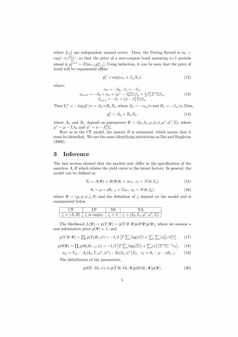
where t are independent normal errors. Then, the Pricing Kernel is mt =

exp(−rt) ξt+1ξt, so that the price of a zero-coupon bond maturing n+1 periods

ahead is pn+1t = E[mt+1pnt+1]. Using induction, it can be seen that the price of

bond will be exponential affine:

pnt = exp(αn + βnXt), (12)

where:α1 = −δ0, β1 = −δ1,

αn+1 = −δ0 + αn + (µ| − λ|0Σ)βn +

12β

|nΣ

|Σβn,βn+1 = −δ1 + (φ− λ|1Σ)βn.

(13)

Then Y nt = − log pnt /n = An+BnXt, whereAn = −αn/n andBn = −βn/n.Thus,

ynt = An +BnXt, (14)

where An and Bn depend on parameters Ψ = (δ0, δ1, µ, φ, σ, µ∗, φ∗,Σ), where

µ∗ = µ− Σλ0 and φ∗ = φ− λ|1Σ.Here as in the CF model, the matrix B is estimated, which means that it

must be identified. We use the same identifying restrictions as Dai and Singleton(2000).

3 InferenceThe last section showed that the models only differ in the specification of thematrices A,B which relates the yield curve to the latent factors. In general, themodel can be defined as

Yt = A(Ψ) +B(Ψ)θt + σet, et ∼ N(0, In) (15)

θt = µ+ φθt−1 + Σut, ut ∼ N(0, Ip) (16)

where Ψ = (µ, φ, σ, ζ, θ) and the definition of ζ depend on the model and issummarized below.

CF LP NS NAζ = (A,B) ζ is empty ζ = λ ζ = (δ0, δ1, µ

∗, φ∗,Σ)

The likelihood L(Ψ) = p(Y |Ψ) = p(Y |θ,Ψ)p(θ|Ψ)p(Ψ), where we assume anon informative prior p(Ψ) = 1, and

p(Y |θ,Ψ) =Qt p(Yt|θt, ψ) = −1/2£TP

i log(σ2i ) +

Pt

Pi(u

2it/σ

2i )¤, (17)

p(θ|Ψ) =Qt p(θt|θt−1, ψ) = −1/2£TP

i log(|Σ|) +P

t(e|t (Σ

|Σ)−1et¤, (18)

uit = Yit −Ai(δ0,Σ, µ∗, φ∗)−Bi(δ1, φ

∗)Xt, et = θt − µ− φθt−1 (19)

The distribution of the parameters,

p(θ|Y,Mt, ψ) ∝ p(Y |θ,Mt,Ψ)p(θ|Mt,Ψ)p(Ψ), (20)

5

cannot be derived analytically, but the Clifford-Hammersley theorem guaranteesthat the recursive sampling of subsets of parameters, obtained from the com-plete conditional distributions, converges to the joint distribution. The subsetsare chosen in a convenient way such that the subproblems have, when possi-ble, analytical solutions and known complete conditional distributions, as is thecase of subproblems 1-3 bellow. These problems correspond to, respectively,an estimation of a VAR model, the variance of known random variables, andthe extraction of unobservable factors from a multivariate dynamic model. Thesubproblem (4) relative to ζ does not have known expression and its distributionwill be derived utilizing the Metropolis-Hastings rejection method (Gamerman,2001, and Johannes and Polson, 2003), with a proposal obtained from a normaldistribution, centered on the value of the previous iteration, and with an arbi-trarily fixed variance such that the acceptance rate is in the interval [0.3, 0.8].The distributions calculated in each step of the algorithm are:

1. (µw, φw) ∼ p(µ, φ|σw, ζw, θw),2. σw ∼ p(σ|µw, φw, ζw, θw),3. θw ∼ p(θ|µw, φw, ζw, σw),4. ζwi ∼ p(ζi|ζw−i, µ, φ,Σ, σ, θ),

We have:Subproblem1: p(µ, φ|σw, ζw, θw) ∼ N((X|X)−1X|X∗, (X|X)−1⊗Σ), whereX = (θw1 , ..., θ

wT−1)

| , X∗ = (θw2 , ..., θwT )| .

Subproblem2: p(σ|µ, φ, ζ, θ) ∼ IG(diag(e|e)), where e = Y −A− BX, andIG is the inverse gamma distribution.Subproblem3: p(θ|µ, φ, σ, ζ) = Q

t p(θt|µ, φ, σ, ζ), where p(θt|µ, φ, σ, ζ) =p(θt|DT ) ∼ N(ht,Ht) is the FFBS algorithm defined in the Appendix.The subproblems 1-3 are common to all models. The subproblem 4 depends

on the definition of ζ. In the case of the LP there is no ζ, and so subproblem 4is not defined.In the case of the CF model, ζ = (A,B) is estimated without restrictions.

Subproblem 4 becomes

(ζ|µ, φ, σ, θ) = (A,B|µ, φ, σ, θ) = N((θw|θw)−1θw|Y, (θw|θw)−1 ⊗ σ2). (21)

In the models NA and NS, the parameter ζ do not have known condi-tional distribution. In this case, its distribution will be obtained through arejection method - Metropolis-Hastings - where the proposal is sampled froma normal distribution centered on the value of the previous iteration, witharbitrarily fixed variance such that the acceptance ratio lies in the interval[0.3, 0.8]: p(ζi|ζi−1, µ, φ, σ, θ) ∼ N(ξki , c) and accepts if p(Y |ξki )−p(θ|ξk−1i ) > u,u ∼ U(0, 1).

6

3.1 Performance Criteria

The models under investigation have a different number of parameters, andhence they must be compared emphasizing forecasting performance or adherenceto data. Gelfand and Ghosh (1998) proposed the minimum posterior predictiveloss (PPL) criterion emphasizing forecasting performance. Spiegelhalter (2002)proposed the DIC criterion emphasizing adherence. Besides those measures,we will calculate Theil’s U statistical measure, which consists of normalizingthe MSE of out-of-sample forecasts and of in-sample adherence with respect tocorresponding measures using random walks.

3.1.1 Minimum posterior predictive loss

For each point of the distribution of the estimators Ψw ∼ (Ψ|Y ) there corre-sponds a forecasting for the yield curve Y | Ψw. Gelfand and Ghosh (1998)proposes a loss function penalizing the expected error E(Y |Ψw) − Y and thevariance of the forecasts Y |Ψw − E(Y |Ψw). In our case, the target variable ismultivariate, so that we take the mean of the expected losses calculated for eachof the maturities. In other words, the criterion is:

PPL =Xi

Xt

¡Y it −E(Y i

t |Ω)¢2+Xi

Xt

1

Nw

Xw

¡E(Y i

t |Ψw)−E(Y it |Ω)

¢2,

(22)

3.1.2 Divergence of Information Criterion (DIC)

Spiegelhalter (2002) proposed a generalization of the AIC criterion based on thedistribution of the divergence D(Ψ) = −2 logL(Ψ):

DIC = E(D(Ψ))− pd = 2E(D(Ψ))−D(E(Ψ)), (23)

where pd = E(D(Ψ))−D(E(Ψ)) measures the equivalent number of parametersin the model, E(D(Ψ)) is the mean of the divergences taken in the posteriordistribution of the estimators and D(E(Ψ)) is the divergence calculated at themean point of the posterior distribution of the estimators.Banerjee et al (2004) claims that LLP and DIC evaluate the fitting and

penalize the degree of complexity of the models, but that the DIC takes intoaccount the likelihood on the space of the parameters and PPL on the predic-tive space. Thus, when the main interest lies is forecasting, the PPL is to bepreferred, whereas when the capacity of the model to explain the data is moreinteresting, DIC should be used.

3.1.3 Theil’s U

When the processes under study have high persistency, the simplest represen-tation, the random walk, frequently adheres to data. This is our case, in which

7

hardly the yield curve suffers abrupt changes. Hence, a direct criterion to eval-uate the results of the model is to compare it to the results of the randomwalk with the same set of information. Theil proposed to make this comparisontaking the ratio between the standard deviation of the errors of the one-stepforecasts and the standard deviation of the first difference of the variable. Inour case, this result is calculated for each maturity, and when necessary it issummarized by the mean value along all maturities. The formula is:

Theil-U =

ÃPt(Yt − bYt|t−21)2Pt(Yt − Yt−21)2

! 12

. (24)

4 ResultsThe performance of the models is evaluated in 3 markets having distinct features.The first one is the DIxPRE Swap contract traded in the Brazilian futures market(BM&F) for many maturities, and is used as an approximation to the termstructure of public bonds traded in the domestic market. The second one isthe market of Sovereign bonds issued by the Brazilian Treasury. We use datatreated by Bloomberg which provides constant maturity zero-coupon bonds. Itis smaller and less liquid than the domestic government bonds market, and,being a sovereign bond depends more directly on the effects of fluctuationsof the perception of risk that agents have about the capacity of the Braziliangovernment to honour those bonds, that is, on credit risk. Finally, the thirdmarket is that of the US Treasury bonds. The Federal Reserve provides free ofcoupon and constant maturity rates.The features of the interest rates market and the availability of data moti-

vated our choice of analyzing the markets with daily frequency. This was partic-ularly important for the Brazilian domestic market, which, like other emergingmarkets, has specific characteristics. It is conditioned to the credit risk of thepublic debt, to the higher volatility of the rates due to macroeconomic instabil-ity, to the vulnerability of the exchange rate, and finally, to interventions of themonetary authorities. In January 1999, Brazil adopted the floating exchangerate regime, which changed the mechanism of the formation of the domesticand foreign interest rates. Consequently, the sample used in the estimationswas [01/1999, 09/2005]. The lower temporal dimension was partly compen-sated with the use of daily data.In the Brazilian sovereign market, the data is available starting in March

1998 and ending in July 2005. For convenience, we analyze the US Treasury forthe same period.The degree of linear dependence among the maturities of the 3 markets was

measured calculating the proportion of the variance that is explained by thefirst 3 principal components of the correlation matrix. The table below suggeststhat the markets have at most 3 sources of independent stochastic variance.

8

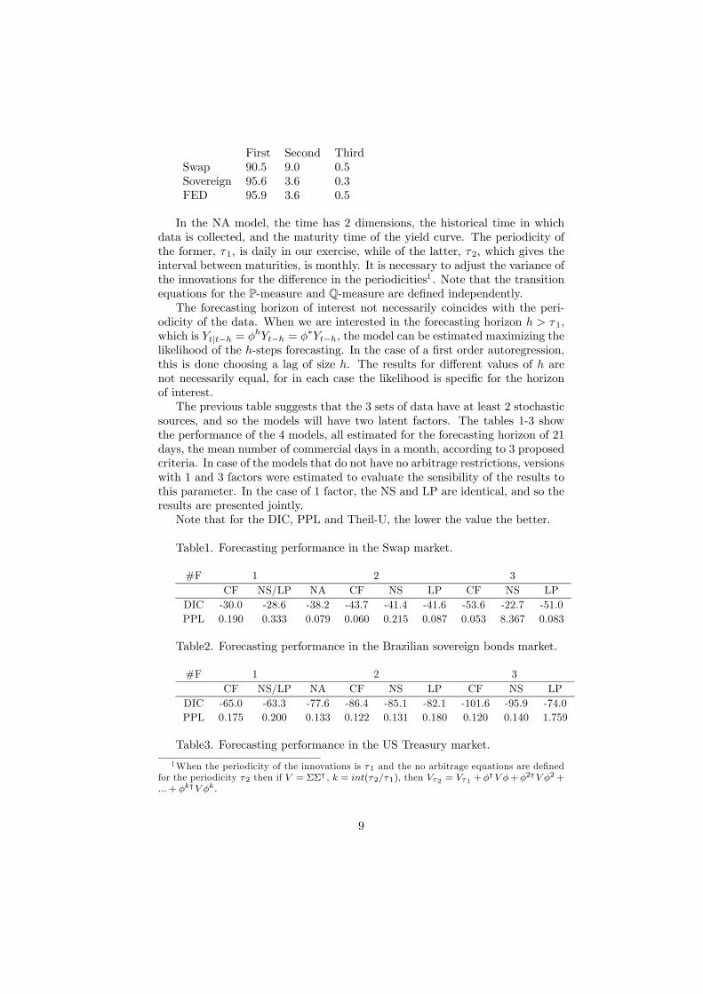
First Second ThirdSwap 90.5 9.0 0.5Sovereign 95.6 3.6 0.3FED 95.9 3.6 0.5

In the NA model, the time has 2 dimensions, the historical time in whichdata is collected, and the maturity time of the yield curve. The periodicity ofthe former, τ1, is daily in our exercise, while of the latter, τ2, which gives theinterval between maturities, is monthly. It is necessary to adjust the variance ofthe innovations for the difference in the periodicities1 . Note that the transitionequations for the P-measure and Q-measure are defined independently.The forecasting horizon of interest not necessarily coincides with the peri-

odicity of the data. When we are interested in the forecasting horizon h > τ1,which is Yt|t−h = φhYt−h = φ∗Yt−h, the model can be estimated maximizing thelikelihood of the h-steps forecasting. In the case of a first order autoregression,this is done choosing a lag of size h. The results for different values of h arenot necessarily equal, for in each case the likelihood is specific for the horizonof interest.The previous table suggests that the 3 sets of data have at least 2 stochastic

sources, and so the models will have two latent factors. The tables 1-3 showthe performance of the 4 models, all estimated for the forecasting horizon of 21days, the mean number of commercial days in a month, according to 3 proposedcriteria. In case of the models that do not have no arbitrage restrictions, versionswith 1 and 3 factors were estimated to evaluate the sensibility of the results tothis parameter. In the case of 1 factor, the NS and LP are identical, and so theresults are presented jointly.Note that for the DIC, PPL and Theil-U, the lower the value the better.

Table1. Forecasting performance in the Swap market.

#F 1 2 3CF NS/LP NA CF NS LP CF NS LP

DIC -30.0 -28.6 -38.2 -43.7 -41.4 -41.6 -53.6 -22.7 -51.0PPL 0.190 0.333 0.079 0.060 0.215 0.087 0.053 8.367 0.083

Table2. Forecasting performance in the Brazilian sovereign bonds market.


DIC -65.0 -63.3 -77.6 -86.4 -85.1 -82.1 -101.6 -95.9 -74.0PPL 0.175 0.200 0.133 0.122 0.131 0.180 0.120 0.140 1.759

Table3. Forecasting performance in the US Treasury market.

1When the periodicity of the innovations is τ1 and the no arbitrage equations are definedfor the periodicity τ2 then if V = ΣΣ| , k = int(τ2/τ1), then Vτ2 = Vτ1 +φ|V φ+φ2|V φ2+...+ φk|V φk.

9


DIC -84.1 -77.4 -102 -110 -104 -100 -128 -118 -122PPL 0.60 2.50 0.27 0.25 0.33 0.79 0.21 0.44 0.25

Tables 1-3 show that:

• The performance of the CF model is always superior to the other models,for the any number of factors and for the 3 sets of data.

• The models with 3 factors are in general better than those with 2 factors,but the improvement is much less when comparing with the 1 factor mod-els. This suggests that in the 3 cases there are at least 2 factors, and thatin some cases a third may be possible to estimate.

• The performance of the NA model is worse than the CF according to2 criteria for the 3 markets. But is similar to the best model when weconsider the PPL criterion.

• The NS is better than the LP or not depending on the market and on thecriterion.

The comparison between the mean squared error (MSE) of the model andof the random walk (rw), the Theil’s U statistic, is a measure of practical util-ity. Models with errors greater than that of the random walk are useless forforecasting. This error depends on the forecasting horizon. In mean-reversionprocesses, the error of the rw tends to grow faster than that of the model withrespect to greater horizons. Tables 4-5 present results of the model CF with 2factors and for 3 markets: 1) the PPL criterion, 2) the mean of the MSE forthe forecasting errors of the model for all maturities in the indicated horizon,3) the mean of Theil’s U statistics computed in-sample, and finally 4) the valueof the out-of-sample Theil-U for all maturities (last 30 observations).Values of out-of-sample Theil-U’s less than 1 are highlighted because it

means the model presented better forecasting performance than the rw.

Table 4. Effect of the forecasting horizon. Swaps.lags 10*PPL 10*MSE In-sample TU

1 0.09 0.03 1.415 0.21 0.09 1.0610 0.33 0.18 0.9921 0.51 0.31 0.94

Out-of-sample Theil Ulags 1 2 3 6 9 12 18 24 361 4.52 1.62 0.99 1.58 1.62 1.82 1.51 1.01 3.935 1.51 0.96 0.93 1.08 0.99 1.03 1.04 1.08 2.2010 0.81 0.70 0.75 1.11 0.96 0.91 0.97 1.13 1.8421 0.52 0.59 0.58 0.94 1.14 1.06 1.11 1.40 2.32

10

The results indicate that:

• When the horizon is 20 times greater, the MSE rises 10 times, less thanwhat would happen with a rw.

• For horizons above 5 days the predictions of the model are better thanthose of the random walk.

Table 5. Effect of the forecasting horizon. Brazilian Sovereign bonds.

lags 10*PPL 10*MSE In-Sample TU1 0.22 0.06 0.995 0.28 0.19 1.0810 0.70 0.31 1.0321 1.15 0.53 0.99


The results show that:

• When horizon is 20 times greater, the MSE is 9 times greater.• Better forecasts are not linked to the horizon, but are linked to maturities[6,24] months.

Table 6. Effect of the forecasting horizon. US Treasury.

lags 100*PPL 100*MSE In-Sample TU1 0.075 0.015 1.035 0.125 0.030 1.1010 0.168 0.048 1.2121 0.251 0.086 1.85


The results show that the model presents a superior forecasting performancewith respect to the random walk only for the short rate and for horizons up to5 days.

11

5 ConclusionWe analyzed with daily data 3 yield curves, the Brazilian domestic market inter-est rate swaps, the Brazilian sovereign bonds and US Treasury bonds, equippedwith 4 models: the common factor model of the time series literature, the affineno arbitrage model of the Finance literature, and 2 models that geometricallydecompose the yield curve, Nelson-Siegel and Legendre polynomials, modifiedto include dynamic effects of the latent components.It resulted that the common factor model, in spite of having a much greater

number of parameters, had better performance according to two criteria, theposterior predictive loss and DIC, related to the predictive and explanatorypower of the model, respectively. Also, the affine model presented inferior butcomparable results. This may be attributed to the complexity of estimation ofthe risk premia.The common factor model was used to evaluate the effect of the forecasting

horizon on the forecasting performance in the 3 markets. Depending on themarket, the model tend to have better results compared to the random walk forlonger horizons.An immediate extension of this work is the incorporation of macro state

variables as Ang and Piazzesi (2003), and evaluate the predictive performanceof the models with and without no arbitrage.

6 References

1. Almeida CIR, Duarte AM, Fernandes CA. Decomposing and Simulatingthe Movements of Term Structures in Emerging Eurobonds Markets, Jour-nal of Fixed Income 1998; 1, 21-31.

2. Ang A, Piazzesi M. A no-arbitrage vector autoregression of term structuredynamics with macroeconomic and latent variables. Journal of MonetaryEconomics 2003; 50, 745-787.

3. Banerjee S, Carlin B, Gelfand A. Hierarchical Modeling and Analysis. forSpatial Data. CRC Press/Chapman Hall; 2004.

4. Dai Q, Singleton K. Specification analysis of term structure of interestrates. Journal of Finance 2000; 55, 1943-78.

5. Diebold FX, Li C. Forecasting the term structure of government bondyields. Journal of Econometrics 2006; 130, 337-364.

6. Duffie D, Kan R. A yield-factor model of interest rates. MathematicalFinance 1996; 6, 379-406.

7. Gamerman D. Markov chain Monte Carlo: stochastic simulation for Bayesianinference. Chapman & Hall: London; 1997.

12

8. Gelfand A, Ghosh S. Model choice: a minimum posteriori predictive lossapproach. Biometrika 1998; 85 1-11.

9. Harvey AC, Forecasting, structural time series models and the Kalmanfilter. Cambridge University Press: Cambridge; 1989.

10. Johannes M, Polson N. MCMC methods for continuous-time financialeconometrics. Working paper 2003.

11. Litterman R, Scheinkman J. Common factors affecting bond returns. Jour-nal Fixed Income 1991; 1, 51-61.

12. Nelson CR, Siegel AF, Parsimonious modeling of yield curves, Journal ofBusiness 1987, Vol. 60, No. 4, 473-89.

13. Rudebusch G, Wu T. A macro-finance model of the term structure, mone-tary policy and the economy. Working Paper 2003; Federal Reserve Bankof San Francisco.

14. Spiegelhalter D, Best N, Carlin B, van der Linde A. Bayesian Measures ofModel Complexity and fit (with discussion). Journal of the Royal Statis-tical Society Series B 2002, 64, 583—639.

15. West M, Harrison PJ. Bayesian forecasting and dynamic models, Springer:NewYork; 1997.

A Appendix: Kalman Filter and FFBS algo-rithm

We present the Kalman Filter and the FFBS algorithm of the Dynamic LinearModel (DLM) in which part of the components are observed (M). Defining

Yt = A+BMMt +Bθθt + et, et ∼ N(0, Iσ),Mt = µM + φMMMt−1 + φMθθt−1 + uMt ,θt = µθ + φθMMt−1 + φθθθt−1 + uθt ,

(25)

we obtain the linear dynamic model

Yt = yt + Fθt + et, et ∼ N(0, Iσ),θt = xt +Gθt + ut, ut ∼ N(0,W ),where yt = A+BMMt,xt = µθ + φθMMt−1,F = Bθ, G = φθθ.

(26)

that can be estimated as follows:

13

Given: (θt−1|Dt−1) ∼ N(mt−1, Ct−1).Prior: (θt|Dt−1) ∼ N(at, Rt),where at = Gmt−1 Rt = GCt−1GT +W.Forecast: (Yt|Dt−1) ∼ N(ft, Qt),where ft = Fat Qt = FRtF

T + σ.Posteriori: (θt|Dt) ∼ N(mt, Ct),where mt = at +At(Yt − ft), Ct = Rt −AtQtA

Tt , At = RtFQ

−1t .

(27)

Once the conditional distribution of (θt|Dt) t = 1..T is obtained, the FFBSalgorithm permits one to obtain a sample of (θt|DT ).

Given: (θT |DT ) ∼ N(mT , CT ).(θt|θt+1) ∼ N(ht,Ht),where ht = mt +Bt(θt+1 − at+1) Ht = Ct −BtRt+1B

Tt Bt = CtG

TR−1t+1.(28)

14

Ipea – Institute for Applied Economic Research

PUBLISHING DEPARTMENT

CoordinationCláudio Passos de Oliveira

SupervisionEverson da Silva MouraReginaldo da Silva Domingos

TypesettingBernar José VieiraCristiano Ferreira de AraújoDaniella Silva NogueiraDanilo Leite de Macedo TavaresDiego André Souza SantosJeovah Herculano Szervinsk JuniorLeonardo Hideki Higa

Cover designLuís Cláudio Cardoso da Silva

Graphic designRenato Rodrigues Buenos

The manuscripts in languages other than Portuguese published herein have not been proofread.

Ipea Bookstore

SBS – Quadra 1 − Bloco J − Ed. BNDES, Térreo 70076-900 − Brasília – DFBrazilTel.: + 55 (61) 3315 5336E-mail: [email protected]

Composed in Adobe Garamond 11/13.2 (text)Frutiger 47 (headings, graphs and tables)

Brasília – DF – Brazil

Ipea’s missionEnhance public policies that are essential to Brazilian development by producing and disseminating knowledge and by advising the state in its strategic decisions.

comparing models for forecasting the yield...

Documents