comparing four different methods for ...nersp.osg.ufl.edu/~ufruss/documents/comparing...

Social Networks 12 (1990) 179-215

North-Holland

179

COMPARING FOUR DIFFERENT METHODS FOR MEASURING PERSONAL SOCIAL NETWORKS *

H. Russell BERNARD * *

University of Florida

Eugene C. JOHNSEN

University of California, Santa Barbara

Peter D. KILLWORTH

Hooke Institute for Atmospheric Research, Oxford

Christopher MCCARTY and Gene A. SHELLEY

University of Florida

Scott ROBINSON

Univ. Metropolitana, Mexico City

1. Introduction

Like many researchers, we want to know the rules that govern the formation of human social networks, their persistence and disap- pearance, and their effects (if any) on human behavior and thought. Even if it turns out that the rules governing social network formation and decay are relatively simple, the outcome of those rules is very complex.

It is so complex, in fact, that at this stage of the effort we are still concentrating on basic questions like: How many people are there in

* This research was supported by a grant from the Anthropology Program and the Measurement

Methods program of the National Science Foundation. The Mexico City data were collected by

Yolanda Hemandez and Rosaria Mata Castrejon.

** Correspondence should be addressed to H. Russell Bernard, Department of Anthropology, University of Florida, 1350 Turlington Hall, Gainesville, FL 32611, U.S.A.

037%8733/90/$3.50 0 1990 - Elsevier Science Publishers B.V. (North-Holland)

180 H. R. Bernard et al. / Measuring personal social networks

people’s social networks? How does the size of those personal networks vary across individuals, across social groups, and across cultures? And what accounts for these variations? At the operational level, how does the number of people whom people know vary according to the type of question or method one uses to generate social networks? In other words, what is the “measurement effect” in acquiring the data that we use for the analysis of social networks?

From the literature it is clear that there are many kinds of networks. Four kinds of networks are frequently discussed. One of these, often called an “emotional support group”, is comprised of just a few intimates. People may call such intimates their “friends”, but that word is also used to refer to a great many others who are not in the emotional support network. The method used to elicit this network usually consists of some query beginning with “who do you” and ending with things like “discuss important matters with” or “talk to when you feel lonely”, etc. Note that the query used determines the list of names elicited, so that any particular query generates an approxima- tion to the network.

Another, usually larger, network is often called the “social support group”. Many of the people in this network are also classified as “friends”, but need not be. These are the people on whom one calls for a variety of favors. Reciprocity is usually a component of such relations, but emotional intimacy need play no part in them. The favors that one asks of the people in this circle are varied and may be relatively trivial or of great importance, but one can always count on the alters to render the favors when asked. The members of this network are elicited by asking a series of questions like: “Who could take care of your house if you went out of town?” or “Who would you borrow a large sum of money from?” Some of these social support questions tend to elicit names of relatives (“Who are the adult members of your household?“) Once again, the network elicited depends on the questions asked.

These two categories of networks (emotional and social support) are embedded in what we can call the “global network”. This network, unlike the others, is well defined. It consists of all the people known to an individual, given a suitable definition of “knowing”. The method of eliciting this network consists of prodding an informant to recall the names of all the people he or she can remember. One method is to ask an informant to carry around a notebook and jot down the names of

H.R. Bernard et al. / Measuring personal social networks 181

people he or she meets over some period (Gurevich 1961; Poole and Kochen 1978). Another method is to present an informant with a representative list of last names from a phone book and to ask for all the names of persons that the informant can remember from his or her own network having those last names. Neither of these techniques actually elicits the global network; they elicit proxies for it.

Many of the people in the global network serve no apparent function other than as conduits of information. Indeed, some of them may not even know your name, even though you know theirs and you believe that they will remember you were you to call them up and introduce yourself. On the other hand, some of the people in the global network do have roles that are not exhausted by the emotional and social support networks mentioned above. Those people who have a given role for an individual constitute another network. One can think of the “network of people who can provide information about job opportuni- ties” or the “network of people who can help your children get into a good college” and so on.

Indeed, some of the roles played by members of an informant’s global network may be defined by researchers in order to elicit part of that network. This is the case with the reverse small-world technique (RSW) (Killworth and Bernard 1978; Killworth et al. 1984; Bernard et al. 1988). In RSW, informants are asked to name those members of their global network whom they could use as carriers of information to persons outside their global networks. We originally conceived of RSW as a dredging technique, or a way to estimate the number and type of people known to an informant. The work of Freeman and Thompson (1989) made it clear that RSW only captures part of the global network.

We assume for this paper that all the commonly used techniques for capturing lists of network members are valid. That is, they produce some subset of the global network which has an entity of its own. How can we determine the relationship between these subsets? Are intimates part of one’s social support network? Does RSW elicit any substantial part of the social support network? If we made a list of our current global network, what part of our social support network would it contain?

These kinds of questions cannot be addressed by data on only one of these networks. We cannot concatenate the data from two different studies on two different sets of informants. What is needed is a study in

182 H.R. Bernard et al. / Meusurrng personal social networks

which the same informants are asked to provide data on the several kinds of networks that have interested researchers.

This paper presents the results of two such studies, one in Jackson- ville, Florida, and one in Mexico City. Section 2 describes the experiment; Section 3 gives some brief details about the informants; Section 4 gives some elementary statistics about the membership of the networks. Section 5 examines the role played by spouses in networks. In Section 6, we apply our earlier analyses to the data generated by RSW. Section 7 looks at the membership of the social support network in more detail, and Section 8 examines the overlaps between the various networks. We conclude with a discussion and suggestions for future work.

2. The experiment

To elicit the network of intimates, we chose a variant of the single- question instrument used by Burt in the General Social Survey of 1985: With whom can you discuss important matters? (Burt 1984). For the social support network, we used a slightly modified version of the instrument used by Fischer and his colleagues in the Northern Cali- fornia Study and published by McCallister and Fischer (1983). The Fischer/McCallister instrument consists of 11 questions:

1. Who would take care of your house if you went out of town? 2. If you work outside of your house, who would you talk to about

work decisions?. 3. Who, if anyone, has helped with household tasks in the last three

months? 4. With whom have you engaged in social activities in the last three

months (such as going to the movies, had over for dinner, etc.)? 5. Who do you talk to about hobbies? 6. Who is your “best friend”? 7. Who do you talk to about personal worries? 8. Who do you get advice from when making important decisions? 9. If you needed a large sum of money, who could you borrow it

from? 10. Who are the adult members of your household, excluding you? 11. Who do you feel especially “close to”?

H. R. Bernard et al. / Measuring personal social networks 183

The RSW instrument is described at length in Killworth et al. (1984). The informant is presented with a list of 500 mythical names of persons in the world. Each name is equipped with a location and an occupation. Four hundred of the names, representing the world, are standard in all RSW experiments. One hundred new names are added to each experiment. These represent the country of the informants. Informants are instructed in the small-world technique (Milgram 1967). They are then told to imagine that each of the names on the RSW list are targets in a small-world experiment. Informants look at the information provided about each target and name the member of their own network whom they believe would be the most appropriate first intermediary to the target. They also tell us whether the target’s location or occupation was more important in making them think of their choice for inter-

mediary. Finally, for the global network, we used a modification of the

method pioneered by Poole in the 1950s (Poole and Kochen 1978) and significantly improved upon by Freeman and Thompson (1989). Infor- mants were presented with a list of 305 last names generated randomly from their local phone book. Each different name has an equal chance of occurring in the list, so that Smith and Wojohowicz have an equal chance of being selected. Informants were asked to list any and all of the people they knew with each last name. (Freeman and Thompson asked for people whom informants had euer known; many of the Jacksonville informants took the question to mean this, but omitted those whom they knew to be deceased.)

Of course, this phone book technique yields the names of only a few persons from each informant. The method for scaling up these names to estimate the size of the global network for an informant is discussed by Killworth et al. (1989).

The four network generators were incorporated as modules into a single, computer-based test, the network suite. Two groups of informants were interviewed, one group in Orange Park, Florida (a suburb of Jacksonville), and one group in Mexico City. In both studies, informants sat at a microcomputer and responded to a series of questions.

Informants were first shown a series of screens that explained the experiment. Next, informants provided some basic socioeconomic and demographic information about themselves, and gave their opinions on two political questions (different, of course, for Jacksonville and Mexico

184 H. R. Bernard et al. / Measurrng personal social networks

City). Informants also were asked how many people they thought they knew in each of four different ways: people with whom they could discuss important matters; people on whom they could call for things like transport, child care, etc.; people who were in their circle of friends, relatives and acquaintances; and people whom they had ever known, throughout their lives. (Anchor values for these were supplied:

Great! Now that we know something about you, we’re ready to begin the first of four

modules. For this part we would like to know the names of all the people with whom you

can discuss important matters. The people named here should be those with whom you can

confide in about topics which are very personal to you. You can use first names, last names

or both. On some modules you will be allowed to use names over again. If you use a choice

more than once, please type their names exactly the same each time.

OK. On the following screen you will see some highlighted boxes for information about

the people with whom you discuss important matters. We would like to know three things:

the choice’s name, the choice’s sex and the choice’s relationship to you (that is, whether

they are a friend, a relative or an acquaintance). Press any key to proceed.

Type the appropriate information in the highlighted box and hit ‘Enter’ to move to the

next box. When you are done, hit the Fl0 key while in the First Name box. The program

will then list all of your choices and give you a chance to add to or delete from the list.

Question: With whom can you discuss important matters?

First Name Last Name

Sex 0

I= Male 2 = Female

F/A/R 0

1 = Friend 2 = Relative 3 = Acquaintance

Fig. 1. Some samples screens from the network suite, as seen by informants.


Type the appropriate information in the highlighted box and hit ‘Enter’ to move to the

next box. When you are done, hit the Fl0 key while in the First Name box. The program

will then list all of your choices and give you a chance to add to or delete from the list.

Current question is: Who could take care of your house if you went out of town?

First Name Last Name

Sex I F/A/R q l=Male 2 = Female

1= Friend 2 = Relative 3 = Acquaintance

Look at the information on the target. When you have a choice enter their name, sex and their

relationship to you. Rank the location and the occupation using 0, 1 or 2 (but not 0, 0 or 1, 1 or

2, 2). If you want to skip this target until later, hit Page Down. Hit F10 for a list of your previous

choices. Hit F8 to see how many you have left.

Target 1, whose name is MARCELLA LEGENDRA, lives in

VOH. NEW CALEDONIA and works as a WATER METER READER.

You would choose as the person you know who is

most likely to know this choice. Your choice’s sex is and their relationship to you is

making your choice.

Fig. 1 (continued).

I You would rank location as 0 and occupation as 0 in importance to

3, 20, 250, and 5000, respectively.) After answering these questions, informants confronted each of the four modules.

Each module was explained in detail before the informant actually began entering the network names. Figure 1 shows how the modules


looked to informants. As informants responded to the questions in the four modules of the suite, the computer logged the information.

Informants took between 4 and 14 hours to complete the task. All but one of the Mexican informants did the suite in their own homes, on a laptop computer that used floppy disks, while just 26 of the Jackson- ville informants did the suite on a laptop. The other Jacksonville informants came to the home of the researcher and took the suite on a desktop machine that contained a hard disk. The floppy disk version took significantly * * longer to administer (7.6 hours, on average compared with 6.1 for the hard disk version) because of the disk access as each entry was logged. (Throughout, we use * * for significance at the 0.01 level or better, and * for the 0.05 level.)

Jacksonville informants who took the suite on a laptop named more * network alters (174) than did those who took the suite on a desktop machine (139). Each time an informant was asked to enter the name of a network alter, the machine asked whether he or she would like to see a list of the alters already named. Some informants who used laptops started out using this facility but soon came to avoid it and entered names from their heads. The disk access required for inter- rogating their already entered list slowed down an already lengthy experiment. So, there was a weak instrument effect, depending on the type of computer used. But it turns out (see below) that the Jackson- ville informants made the same number of module 3 (that is, RSW) choices as all previous U.S. informants, so that using computers does not have a strong effect on the data.

Most informants required more than one sitting to respond to all four modules. The program was designed so that informants could stop at any time after the second module and return at a later time to continue with the suite.

At the end of the suite, the informant was presented with a list of all the names that he or she had entered during the session. The computer asked the informant to scan the list of network alters that had been mentioned and decide whether any of them were duplicates of one another. From previous studies, we know that informants name many of their network alters more than once. They might say that Mary Belski is a person with whom they discuss important matters (module 1) and is also their best friend (module 2, question 10). Then later, in module 3, they might name “Mary” (with no last name) as the person to whom they would pass a folder for every target in Australia. Mary


Belski and “Mary” are the same person to the informant, but would initially be logged by the computer as different individuals. The final part of the suite, then, allowed the informant to approve a list of unique network alters.

Fifteen of our informants in Jacksonville did not type. They responded verbally to the queries on the computer screen and the researcher typed in the answers. (This also occurred in Mexico, but we have no record of who the informants were who had to be helped in this way.) The researcher happened to have been a professional typist at one time, so informants who were helped in this way took less ** time (5.3 hours, on average) than did informants who did the suite on their own (6.7 hours). On the other hand, there was no significant difference in the number of alters generated by informants who were helped compared with those informants who were not.

By accident, the information about sex and relationship of module 4 choices for the Jacksonville informants was lost. We were able to obtain estimates of the sex of many of these choices from their names for the purposes of descriptive statistics, but the information is otherwise not present.

3. The informants

The average age of the Jacksonville informants was 37 years (with range 18 to 70). Informants in Mexico were younger (33 years, range 19 to 68). There were 49 male informants in Jacksonville and 49 female informants. In Mexico, there were 49 male informants and 50 females. The income of the Jacksonville informants ranged from less than $5,000 to more than $75,000 per year, with 70% between $25,000 and $75,000. In Mexico City, we measured income in multiples of “salario minimo”, or minimum daily wage. The range was from less than minimum wage to more than five times that figure.

In Jacksonville, 54% of the informants had completed high school, and 35% had a bachelor’s degree. In Mexico City, 13% had completed primary school, and 17% finished the equivalent of junior high, 20% completed high school, and 38% had completed some professional school or university.

In both studies we assessed occupation level on a 1 to 3 scale, from low to high. Informants were roughly evenly distributed among the three levels.


4. The number of choices

Modules 2 and 3 differed from modules 1 and 4 in that informants could mention the same person more than once. Thus, we can count both the total number of alters and the number of different alters generated by each informant for each module and over all four modules. The total number of alters and the number of different alters are therefore the same for modules 1 and 4. Recall that module 4 yields only a few persons, by its nature, but that the number of module 4 choices can be scaled up to estimate the total network of an individual informant (see Killworth et al. 1989).

Table 1 shows the mean number of choices for each of the modules in Jacksonville and Mexico City (hereafter J and MC). The distribution of the number of choices among informants is shown in Figure 2. The shape of the J distribution is very similar to those for other U.S. informants (Bernard et al. 1988). The mean for J on module 1 is 6.88, significantly higher than the maximum of 5 imposed on respondents to the 1985 General Social Survey. The mean number of different choices for J on module 2, 21.82, is very close to the average of 18.5 reported by McCallister and Fischer (1983). The total number of choices for module 2 is naturally higher for both J and MC, since choices are repeated among the 11 questions.

Table 1

Number of choices generated

Module 1

Module 2

(number of

different choices)

Module 2

(total number

of choices) Module 3

Module 4

Total no. of

different choices generated

Jacksonville

6.88 (4.89)

21.82 (16.66)

46.36 (27.51) 128.66 (67.58)

11.51 (11.32)

148.31 (69.41)

Mexico City

> ** 2.95 (2.66)

> ** 10.05 (6.45)

>> ** 25.68 (11.86) > ** 76.52 (79.06)

>> ** 4.20 (7.66)

>3 ** 81.55 (83.34)

Notes: Numbers in parentheses indicate standard deviations. z+ or < indicate significant

differences between the two columns.


The number of different choices for module 3 rises again, to 129 for J and 77 for MC. The J value is almost identical to the values for U.S. informants found in previous RSW experiments (Gainesville, 134;

MC

O-3 4-7 6.11 12-15 16-19 20-23 24-27 28-31 32-35 36-39

Number of choices in module 1

50

40

30

20

10

0 7

5 15 25 35 45 55 65 75

MC


Fig. 2(a). Distribution of numbers of choices in module 1, for the J and MC informants.

Fig. 2(b). As (a), but for module 2.

H. R. Bernard et al. / Measuring personal social networks

MC

20 60 100 140 180 220 260 300 340 380


Fig. 2(c). As (a), but for module 3.

420

Provo, Utah, 144; Bernard et al. 1988), while that for MC is the smallest value we have found so far. The 305 phone book names elicited over 11 different choices for J informants, against 4 for M informants. The J value is a little smaller than that found for Orange County students by Freeman and Thompson (1989). If the values 11 and 4 are scaled up by methods given in Killworth et al. (1989), estimates of total network size are 1,391 and 429, respectively.

In all cases in Table 1, J informants made more * * choices than M informants.

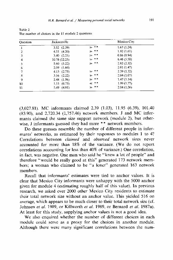
Table 2 examines the number of choices generated by each of the 11 questions in module 2. Question 6 (“best friend”) yielded two choices per informant in both data sets. Not surprisingly, J informants reported fewer ** adult members of their household (question 10). Otherwise, J informants made more * * choices than MC informants. This trend - that MC informants make fewer choices than J informants - will continue throughout this paper.

Recall that informants were asked to guess the number of people whom they know (or knew) in various ways. Despite the guidelines given (3, 20, 250, and 5000), both J and MC informants made estimates which varied from these values. J informants claimed to know, on average, 3.52 (s.d. 1.57), 10.93 (8.70), 203.28 (144.87), and 5,023.72


Table 2 The number of choices in the 11 module 2 questions

Question Jacksonville

1 3.52 (2.39)

2 4.15 (4.20) 3 3.40 (2.21) 4 10.78 (12.25) 5 5.60 (5.22) 6 2.09 (1.60) 7 4.13 (2.75) 8 3.56 (2.22) 9 2.48 (1.96)

10 1.15 (0.73) 11 5.49 (4.81)

Mexico City

>> ** 1.67 (1.24) > ** >> ** >> ** >> **

> ** z- **

>> **

<< **

>> **

1.92 (1.61) 0.86 (0.94) 6.46 (5.50) 2.82 (2.32) 2.01 (1.47) 2.39 (1.32) 2.04 (1.07) 1.47 (1.14) 1.99 (1.77) 2.04 (1.26)

(3,027.81). MC informants claimed 2.39 (1.03), 11.95 (6.39), 101.40 (83.90), and 2,720.34 (1,757.46) network members. J and MC informants claimed the same size support network (module 2), but otherwise, J informants guessed they had more * * network members.

Do these guesses resemble the number of different people in informants’ networks, as estimated by their responses to modules 1 to 4? Correlations between claimed and observed network sizes never accounted for more than 18% of the variance. (We do not report correlations accounting for less than 40% of variance.) One correlation, in fact, was negative. One man who said he “knew a lot of people” and therefore “would be really good at this” generated 173 network members; a woman who claimed to be “a loner” generated 163 network members.

Recall that informants’ estimates were tied to anchor values. It is clear that Mexico City informants were unhappy with the 5000 anchor given for module 4 (estimating roughly half of this value). In previous research, we asked over 2000 other Mexico City residents to estimate their total network size without an anchor value. This yielded 516 on average, which appears to be much closer to their total network size (cf. Johnsen et al. 1989, or Killworth et al. 1989, or Bernard et al. 1987a). At least for this study, supplying anchor values is not a good idea.

We also enquired whether the number of different choices in each module could serve as a proxy for the choices in another module. Although there were many significant correlations between the num-


bers of different choices across modules, none accounted for more than 28% of the variance; some were again negative. So knowing the size of one network does not usefully predict the size of another.

It proved impossible to predict the numbers of different choices in any network by socioeconomic variables about informants. However, some of the J informants were or had been in the military. We proposed that informants who had moved frequently might have larger networks because they had met more people. Although not a perfect proxy for frequent movement, membership in or connection with the military can be tested against total network size. The mean total network size of J informants who were either themselves currently in the military, or had spouses who were, was 179; the remainder had 142. The difference was significant *. A more accurate estimate of how mobile informants had been during their lives may prove to be an important predictor of network size.

4. I. Gender differences

Table 3 shows differences between male and female informants in the number of different choices they made for the four modules. There are no differences for the J informants. Female MC informants made more * different choices in modules 2 and 4 (they actually made more choices in all the modules).

Now consider the gender of the choices. We have found consistently in our RSW studies that informants preferentially make male choices (around 63-70s cross-culturally). This differs from the findings on support networks which consistently show a preference to select the

Table 3 Number of choices in the modules by gender of informants

Module Jacksonville Mexico City

Males

(49)

Females

(49)

Males

(49)

Females

(50)

1 6.84 6.92 2.59 3.30

2 23.08 20.36 8.47 < * 11.60

3 125.14 132.18 66.55 86.28 4 11.67 11.35 2.53 < * 5.84


Table 4 Different choices by sex and relationship

(a) Percentages (average percentages)

Module Jacksonville Mexico City

Male choices 1: 2: 3: 4:

Female choices 1: 2: 3: 4:

Friends 1: 2: 3: 4:

Relatives 1: 2: 3: 4:

Acquaintances 1: 2: 3: 4:

45 (24) 47 (32) 51 (18) 47 (17) 63 (11) >> ** 57 (11) 6.5 (23) 59 (32)

55 (24) 53 (32) 49 (18) 53 (17) 37 (11) -=z ** 43 (11) 35 (23) 41 (32)

48 (26) 2s ** 32 (36) 50 (20) 46 (29) 37 (22) 45 (35) _ 30 (41)

50 (25) 40 (19)

17 (8) _

3 (8) 1 (6) 10 (14) 8 (11) 46 (23) > ** 27 (25) _ 65 (42)

< ** 61(37)

46 (27) -=x ** 27 (25)

5 (17)

(b) Actual counts (average counts)

Male choices 1: 2: 3: 4:

Female choices 1: 2: 3: 4:

Friends 1: 2: 3: 4:

3.09 (2.64) B ** 1.35 (1.51) 11.32 (11.02) >> ** 4.61 (3.45) 78.15 (43.13) >> ** 42.92 (44.43) 7.11 (6.49) >> ** 1.88 (3.86)

3.76 (3.34) 2> ** 1.55 (1.41) 10.18 (7.05) > ** 5.26 (3.65) 47.70 (28.61) 2, ** 31.48 (32.02) 4.45 (5.37) >> ** 1.73 (3.22)

3.50 (3.60) > ** 11.36 (11.90) xi, **

45.77 (37.31) >> **

1.09 (1.77) 4.75 (4.72)

32.99 (41.66) 0.69 (1.96)

194 H.R. Bernard et al. / Measuring personal social networks

Table 4 (continued)

(b) Actual counts (average counts)

Relatives

1:

2:

3:

4:

Acquaintances

1:

2:

3:

4:

3.11 (2.21) > ** 1.76 (1.51)

7.73 (4.96) >> ** 4.31 (3.38) 18.86 (9.29) 16.57 (16.53)

_ 0.26 (1.02)

0.23 (0.82) > * 0.05 (0.33) 2.41 (3.76) > ** 0.82 (1.45)

61.23 (49.73) >> +* 24.85 (43.16)

_ 2.66 (5.24)

No@: estimates of the unknown J module 4 values from what data we could retrieve using

overlaps with module 3 show similar values to the MC data: 28, 3, and 69 for friends, relatives,

and acquaintances, respectively. The percentages reported in (a) are means of percentages, and so

do not compare directly with (b).

same sex of choice as the informant (see below). Table 4 shows the distribution of choices by their sex for the different modules.

We see that the behavior of informants in making choices differs between modules and between cultures. Certainly many differences, either in percentage or number of choices, are significantly different between Jacksonville and Mexico City. In percentage terms informants in J and MC make similar amounts of male and female choices except for module 3 (RSW).

The difference between percentages and actual counts is very interesting. The amount of male choices is always larger for J informants whether measured by percentage or actual counts (the difference is always significant for the counts). Female choices, however, are frequently larger in MC in percentage terms, but larger in J for actual counts. This means that the larger number of choices in J provides a larger number of female choices, although this number can be smaller in percentage terms than for MC. Within cultures, there are fewer differences in gender usage. In modules 1 and 2, female choices are usually more likely than males, but not significantly so. For RSW (module 3) more * * male choices than female choices occurred. The same is true for module 4, but only for J informants. So we find a change from female to male choices as the size of the relevant network increases.


Table 5 Occurrences of different choice by sex of informant and choice

Module

1: Male choices

Female choices Significance

2: Male choices Female choices Significance

3: Male choices Female choices Significance

4: Male choices

Female choices Significance

Jacksonville Mexico City

Informants Informants

Male Female Male Female

394 212 116 150

274 462 132 172 **

1381 836 448 461 843 1151 336 669

** **

8269 7047 3835 4617

3675 5673 2564 3633 ** **

366 293 156 321

161 255 92 248 **

The result for RSW for J informants is in agreement with all previous estimates (e.g. Bernard et al. 1988), which show the 63-70% figure of males mentioned above. The percentage of males in module 3 for MC (57%), while still more than female choices, is the lowest we have encountered. The difference between this figure and the 64% for Gainesville - or any other of the four U.S. populations we have studied, for that matter - is significant * *. These results, then, suggest three levels of reliance on males in RSW: a low value of 57% for Mexican informants; a medium value of 63-64% for U.S. informants; and a high value of 71% for Ponapeans. We have no straightforward explanation for this finding.

Splitting the data by sex of informant and by choice permits a direct comparison with results from other studies of support networks. Table 5 shows contingency tables for this case. There are some differences from Table 4. In modules 1 and 2, there is a strong tendency * * for the choice to be the same sex as the informant, with no significance only for MC modules 1 and 4. (J informants choose the same sex on 64% of all different choices for module 1, and 60% for module 2; MC informants choose only 51% same sex on module 1, and 57% for module 2.) This agrees well with the figure of 59% by McCallister and Fischer (1983). In module 3, males were chosen more * * than females by both sexes: 62% for J, 58% for MC. (The differences between these figures

196 H.R. Bernard et al. / Measuring personal social networks

and those in the previous table demonstrate the many possible averaging techniques.) Module 4 shows a preference * * for males (61%) for J, but the 59% males in MC was not significant.

4.2. Relationships of choices

The two cultures differed significantly in their usage of friends, relatives and acquaintances in the four modules. For example, MC informants chose proportionately more * * family in their emotional support network (module l), and proportionately less * * friends, than did J informants. The latter almost always chose more * * friends, relatives and acquaintances than did MC informants, reflecting the larger overall counts.

The amount of friends, relatives and acquaintances in the four modules also varies with increasing module number (and hence network size). Table 4 shows this clearly. J informants record proportions of both friends and relatives which decrease with module, while the proportion of acquaintances increases. The actual numbers of different choices in these categories rises due to the increasing total number of different choices with module, of course, as is also shown in Table 4. MC informants are very similar in this regard, save that the proportion of friends remains constant between modules 2 and 3.

Finally, we further split choices into the six categories of male friends, male family, etc., and splitting informants by their sex. The tables are too numerous to present. Significant differences exist between cultures, between the sexes of informants, and between modules. The sign of the differences follows those discussed above. There are some strong differences between J and MC informants, too. For example, male and female J informants differed consistently in their usage of family, males, and females, with female informants choosing more * * females than male informants did; more * * family; more * * female friends; etc. While there is a tendency for the female MC informants in these directions, there were no significant effects.

5. Spouses

When people get married, they may acquire an entirely new set of network contacts. However, the constraints of marriage could also lead


to the loss of acquaintance networks, so marriage could either increase or decrease informants’ total network size. Seventy-four of the J informants, and 38 of the MC informants were married. We examined the effect of being married on total network size - that is, the cumulative number of different network choices made in modules 1, 2, and 3 (no spouse occurred in module 4 because the list of names we used simply did not contain the last names of any of our informants).

Being married had no significant effect on total network size for either J or MC informants. Nor was there any significant difference between married and unmarried informants in the size of any of their networks for the individual modules.

This lack of significant difference continues if we split the informants by sex, and their choices by sex and relationship. We only found two significant differences for J informants: female J informants with spouses chose more * females overall (68) than those without spouses (50), and both sexes showed differences * in choice of relatives (not surprisingly, people acquired more relatives when they married).

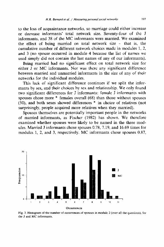
Spouses themselves are potentially important people in the networks of married informants, as Fischer (1982) has shown. We therefore examined whether spouses were likely to be named in the three modules. Married J informants chose spouses 0.78, 7.19, and 16.69 times for modules 1, 2, and 3, respectively. MC informants chose spouses 0.87,

1 2 3 4 5 6 7 8 9 10 11

occurrences Fig. 3. Histogram of the number of occurrences of spouses in module 2 (over all the questions), for the J and MC informants.


6.53, and 11.00 times for the three modules. These values do not differ between the cultures. However, all values are much * * higher than would occur by the chance selection of any network member. Thus, spouses are preferentially chosen for membership of all networks examined. The likelihood of spouses being used in a network decreases with module number (so that spouses occur relatively more frequently

1 .o

0.8

0.6

& .+ t; e

L 0.4

0.2

0

l J OMC

I 1 I / I I I I I 1

1 2 3 4 5 6 7 8 9 10 11

Question

1. Who would take care of your house if you went out of town? 2. If you work outside of your house, who would you talk to about work

decisions? 3. Who, if anyone, has helped with household tasks in the last three

months? 4. With whom have you engaged in social activities in the last three months

(such as going to the movies, had over for dinner, etc.)? 5. Who do you talk to about hobbies? 6. Who is your “best friend”? 7. Who do you talk to about personal worries? 8. Who do you get advice from when making important decisions? 9. If you needed a large sum of money, who could you borrow it from?

10. Who are the adult members of your household, excluding you? 11. Who do you feel especially “close to”?

Fig. 4. The number of occurrences of spouses in each of the 11 module 2 questions, for the J and MC informants, averaged for those informants with spouses.


in emotional and support networks). Spouse occurrence in module 3, though significant, remains a rare occurrence (3% at most).

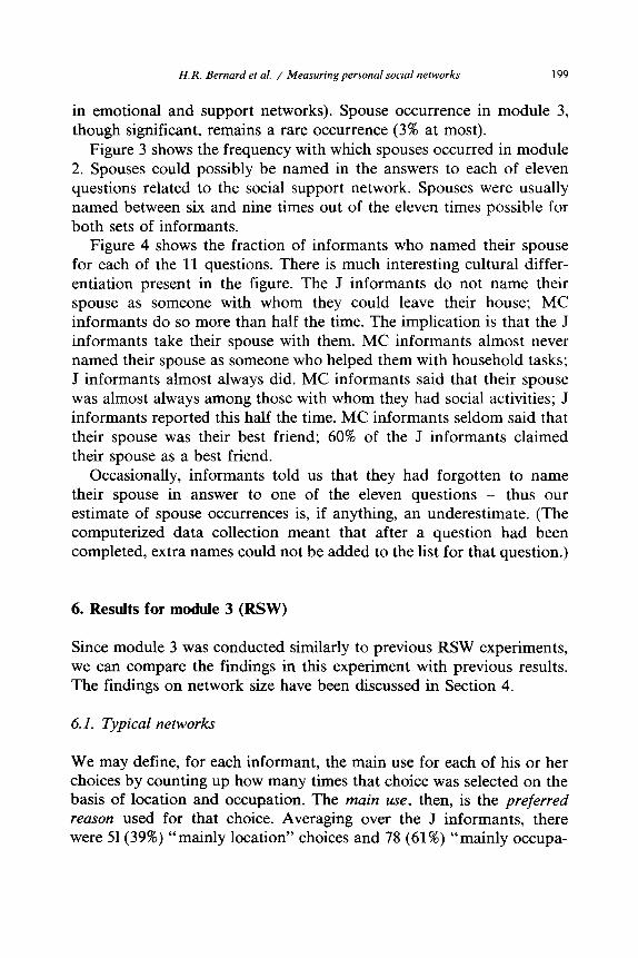
Figure 3 shows the frequency with which spouses occurred in module 2. Spouses could possibly be named in the answers to each of eleven questions related to the social support network. Spouses were usually named between six and nine times out of the eleven times possible for both sets of informants.

Figure 4 shows the fraction of informants who named their spouse for each of the 11 questions. There is much interesting cultural differ- entiation present in the figure. The J informants do not name their spouse as someone with whom they could leave their house; MC informants do so more than half the time. The implication is that the J informants take their spouse with them. MC informants almost never named their spouse as someone who helped them with household tasks; J informants almost always did. MC informants said that their spouse was almost always among those with whom they had social activities; J informants reported this half the time. MC informants seldom said that their spouse was their best friend; 60% of the J informants claimed their spouse as a best friend.

Occasionally, informants told us that they had forgotten to name their spouse in answer to one of the eleven questions - thus our estimate of spouse occurrences is, if anything, an underestimate. (The computerized data collection meant that after a question had been completed, extra names could not be added to the list for that question.)

6. Results for module 3 (RSW)

Since module 3 was conducted similarly to previous RSW experiments, we can compare the findings in this experiment with previous results. The findings on network size have been discussed in Section 4.

6.1. Typical networks

We may define, for each informant, the main use for each of his or her choices by counting up how many times that choice was selected on the basis of location and occupation. The main use, then, is the preferred remon used for that choice. Averaging over the J informants, there were 51(39%) “mainly location” choices and 78 (61 W) “mainly occupa-

200

0.8

0.1

H. R. Bernard ei al. / Measuring personal social networks

a

I I 8 I I I

1 2 3 4 5 6 7

+ Mormon

0 Ponape

l Gainesville

0 Jacksonville

n Mexico City

0 Paiutes

Occupation level of targets

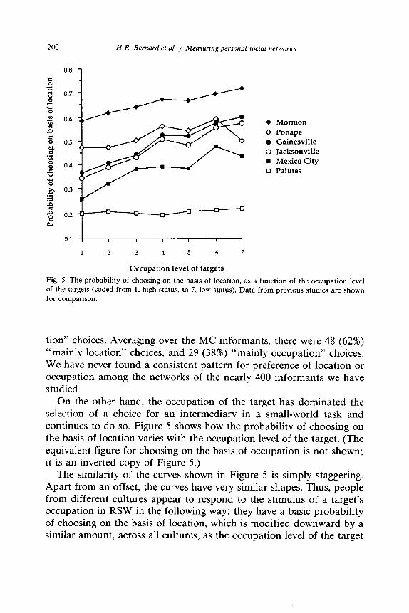
Fig. 5. The probability of choosing on the basis of location, as a function of the occupation level of the targets (coded from 1, high status, to 7, low status). Data from previous studies are shown for comparison.

tion” choices. Averaging over the MC informants, there were 48 (62%) “mainly location” choices, and 29 (38%) “mainly occupation” choices. We have never found a consistent pattern for preference of location or occupation among the networks of the nearly 400 informants we have studied.

On the other hand, the occupation of the target has dominated the selection of a choice for an intermediary in a small-world task and continues to do so. Figure 5 shows how the probability of choosing on the basis of location varies with the occupation level of the target. (The equivalent figure for choosing on the basis of occupation is not shown; it is an inverted copy of Figure 5.)

The similarity of the curves shown in Figure 5 is simply staggering. Apart from an offset, the curves have very similar shapes. Thus, people from different cultures appear to respond to the stimulus of a target’s occupation in RSW in the following way: they have a basic probability of choosing on the basis of location, which is modified downward by a similar amount, across all cultures, as the occupation level of the target


rises. (The correlations of each curve in Figure 5 are significantly * *

positive.) Note the especially close similarity between the curves for Gaines-

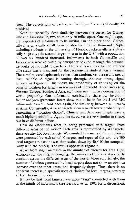
ville and Jacksonville, two cities only 70 miles apart. One might expect the responses of informants to be similar. On the other hand, Gaines- ville is a physically small town of about a hundred thousand people, including students at the University of Florida. Jacksonville is a physically huge city (the second largest in area in the U.S.) with a population of over six hundred thousand. Informants in both Gainesville and Jacksonville were recruited by newspaper ads and through the personal networks of the field researchers. The field researcher for the Gaines- ville study was a man, and for the Jacksonville study it was a woman. The samples were haphazard, rather than random, yet the results are, at least, reliable. A signal is coming through. Another strong signal appears in Figure 6. This shows the probability of choosing on the basis of location for targets in ten areas of the world. These areas (e.g. Western Europe, Southeast Asia, etc.) were OUT intuitive description of world geography. Our informants consistently share our intuition; factor analyses (presented later) show this to be so for the J and MC informants as well. And once again, the similarity between cultures is striking. Consistently, African targets show a much lower probability of generating a “location choice”; Chinese and Japanese targets have a much higher probability. Again, the six curves are very similar in shape, but have different offsets.

How do informants react to being presented with targets from different areas of the world? Each area is represented by 40 targets; there are also 100 local targets. We counted how many different choices were generated by each set of 40 targets, and repeated this with the 100 local targets (this count was then scaled down by 40/100 for compata- bility with the others). The results appear in Figure 7.

Apart from slight increases in the number of choices for area 1 (N. America) for the U.S. informants, the number of choices stays fairly constant across the different areas of the world. More surprisingly, the number of choices generated by local targets does not show an obvious increase over the other areas, and frequently drops. Thus, there is no apparent increase in specialization of choices for local targets, contrary at least to our intuition.

It may be that local targets have more “tags” connected with them in the minds of informants (see Bernard et al. 1982 for a discussion).

202 H. A. Bernard et al. / Measuring personal social networks

0.6

0.4

0.2

0.0 ~1 I I I I I I I I 1

I 2 3 4 5 6 7 8 9 10

l Momon 0 Ponape l Gainesville 0 Jacksonville l Mexico City 0 Paiutes

Area of world

Fig. 6. The probability of choosing on the basis of location as a function of the area of the world a target lives in. Data from previous studies are shown for comparison.

These tags might include where the target’s children go to school, what hobbies the target has, etc. Such tags were not supplied to informants in this experiment, the only information given being target’s location and occupation. However, the Gainesville informants were given four other pieces of information about the (same) targets and yet their data look very similar, with no dramatic increase in choices for local targets.

As in our previous studies, we attempted to predict whether an informant would make a male or a female choice, given information about the target and the informant. The finding continues that the best guess is that an inform~t will choose a male. We also tried to discriminate between friends, relatives and acquaintances in a similar manner. (In our previous studies, we could not differentiate between friend and acquaintance. In those cases, friend was the best guess.) It was possible to improve slightly on the guess of friends in the present


l Mormon 0 Ponape l Gainesville 0 Jacksonville n Mexico City 0 Paiutes

Area of world Fig. 7. The number of different choices produced by informants for 40 targets in each area of the

world, including local targets.

studies, from 39% to 43% for J, and from 48% to 54% for MC. These improvements are far from dramatic.

6.2. Top choices

We have introduced elsewhere the concept of an informant’s top choice, i.e. that choice used more often than any other. Top choices continue to be preferentially male (70% for J, 72% for MC, in line with our other findings - although the percentages vary widely between all the cultures studied so far). Top choices were most likely to be classified as friends (42% for J, 55% for MC). They were used for many targets (12.6% of all targets were accounted for by the top choice for J informants, 9.1% for MC). They continued to be mainly used for location (74% for J, 54% for MC).

204 H. R. Bernard et al. / Measuring personal socral networks

Table 6

Location factor categories

Categories Jacksonville Mexico City

U.S.S.R.

China

Latin America

India/Pakistan

Australia

New Zealand/Pacific

Islands

U.S.A.

Far East

India/Pakistan

U.S.S.R.

W. and E. Europe

(4 Cmk Island

Honduras

India India

Surinam TOllga Kuwail

Bangladesh India

BUIlTId Bhutan

Guam Pakistan

Indonesia philiPPInesIndonesia

rakist

Thailand / Kampuchea I Vietnam I

Tma I / h

Samoa M Cook Is.

N. Zealand New Caledoniz.

Fig. 8(a). Schematic multidimensional

targets)

2.0 Belize

Columbia panarm I%“.XM

Argentina

1.5 Brazil

Nicaragua

Costa Rica Nambia

Nicara%ize

Ecu do?@=’ 8 cuador Mexico

1.0 PalXgUay Guyana

Yel?U?ll Zaire

Ecuador Argentina

Mauntania

0.5

zmalia Libya

Central Afr. Rep. Nigena

Algeria, Libya E $ain I

‘Caled0nm France 1 Italy 0.5 1.0 1.5 2.0

CYPlS Greece

-0.5 Lebanon HWFY

CzechosIovakia Ialawi Iran Greenland USSR Finland

USSR USSR

itmia France E.Gemny uba R&3’pt Grexe

Belgium

-1.0 Finland

Netherlands USSR Scotland Yugoslavia

Iceland Switzerland Netherlands

Wales Wales YUgOSIWia Norway

-1.5

?tlWll

and England

-2.0

England

Irvland

scaling: Jacksonville informants (a sample of the 450


(b) 2.0

+ 1.5 Tonga

Malawi Burq Faso

Namibia Singapk

Hong Kong -- I.0 China

China Bhr tan

Singapam Thailand N. Zealand

China Kampuchea Philippines

oma,%?%pakIs~yew Hebrides

Mauritania __ N. Guinea Pakistan

USSR USSR USSR USSR

Solomon Is.

-2.0

I cod$ I.% BN ei

I I _, ,5 Haiti

USA I&? Caledonia -“‘5

Dom RePvS$reen,and USA USA USA

Canada Samoa

Canada USA

0.5 hdial .O Chad 1 .E 2.0 New Guinea Chad

AusmIia AUStL?& Thailand

-- -0.5Austmlia USSR

Aurtra~mICelan&dan

1 - Mali

AUSh-I.3

Jamaica Norway South Africa

Canada

Cook Is.

Fig. 8(b). As for (a), but for Mexico City informants.

The third most used choice for MC informants, and most of the less used choices thereafter, were chosen more often on the basis of occupation. J informants showed the same structure, although this did not start until the tenth most frequently used choice. This pattern is consistent across the cultures we have studied.

6.3. Factor analysis and multidimensional scaling

As a further attempt to understand how informants perceive the information about targets (here only location and occupation), we used


the technique of Killworth et al. (1984) to provide data for factorings and multidimensional scalings of the targets. Briefly, the similarity of any two targets is proportional to the number of informants who made the same choice for that pair of targets (if that choice was made on the basis of location). The resulting categories of targets’ location are given in Table 6. Note that the factoring does not include the 100 local targets, nor the 40 targets from the area of the world occupied by the informants.

Informants continue to divide the world into the same pieces no matter what their culture. Not only the same main divisions occur (e.g. U.S.S.R.), but also the outliers in the factorings remain similar across cultures (so that Estonia is an outlier on the U.S.S.R. factor).

Multidimensional scalings provide a visual representation of these factors. Figure 8 shows the outcome. Although the distribution of the countries differs, the clustering of the countries into perceived groups is similar between cultures, as indicated from the factor analysis.

7. The module 2 questions

In this section we examine the responses to the 11 questions in module 2 in more detail.

The mean number of responses to the 11 questions is shown in Figure 9. Jacksonville informants made 22 different choices overall on module 2, compared with 10 for MC informants. This larger J response is repeated for all questions except 10 (adult members of household). Notice how the ratio of J to MC figures varies between questions. For example, MC informants reported that very few people (0.86) had helped recently with household tasks, compared with 3.40 for J informants. On the other hand, the figures for best friends (question 6) are indistinguishable: both J and MC informants have two best friends.

What kinds of people are chosen in module 2? We have already seen that these are preferentially female and friends. Figure 10 shows the proportion of male choices used in the 11 questions. Although MC informants mentioned less than one person who had helped them with household tasks, almost all were female; of the almost four people who had helped J informants, however, almost half were male. These findings can be described as follows: females take care of houses if one leaves town, and help with household tasks (in MC only); males discuss


8 -

6 -

OI I I I I I I I I I I

1 2 3 4 5 6 7 8 9 10 11

Question

Fig. 9. Number of responses to the 11 questions in module 2.

0.8

0.7

0.6

$ z 0.5 E

% G 0.4

.z

T-z rt 0.3

0.2 l Male fraction (MC)

0 Male fraction CJ)

0.1

0 I I I , I I I I I I I

1 2 3 4 5 6 7 8 9 10 11

Question

Fig. 10. Fraction of males in module 2 questions.

.J 0 MC


Table 7

Numbers of friends, relatives and acquaintances in module 2 questions

Question Jacksonville Mexico City

8

9

10

11

fr rel ac

2.08 1.15 0.26

2.38 1.34 0.75 1.14 0.87

0.63 2.80 0.13 0.25 0.86

6.51 3.32 1.04 3.98 2.79

3.35 1.74 0.54 1.72 1.13

1.29 0.88 0.00 1.65 0.43

1.88 2.23 0.05 1.15 1.32

1.33 2.13 0.07 0.91 1.21

0.51 2.16 0.00 0.60 0.85

0.08 1.23 0.00 0.14 2.17

1.94 3.57 0.03 0.76 1.33

fr

0.54

rel

1.31

ac

0.06

0.24

0.39

0.18

0.09

0.00

0.00

0.01

0.19

0.06

0.01

Note: The averages are taken only over those informants who provided data for each of the

module 2 questions.

work decisions, and loan money. Other activities are shared fairly equally between males and females in both cultures.

Very few acquaintances are mentioned by informants for any module 2 question. The differences between J and MC informants on these questions is usually significant, and relates to how they use friends and family for social support. Table 7 shows the amounts of friends, relatives, and acquaintances cited in each of the 11 questions. Again, most differences between J and MC are significant * *, since J informants made more choices altogether. MC informants only claim more * friends than J informants for question 6 (best friend). Conforming to cultural expectations, MC informants only claim more * * relatives than J informants for question 10 (adult members of household).

The questions used to elicit the social support network are many and varied. Some, such as “ the adult members of an informant’s household”, seem to be in a different category from “those with whom an informant would discuss personal worries”. Since these questions have been used by social researchers, it is of interest to see whether there is any natural clustering of the questions: whether some are affective, or some are instrumental, or what. We can define a similarity matrix between the 11 questions just as we did for targets in module 3. The similarity between any two questions is the number of times informants mentioned the same person for both questions.


Fig. 11(a). The results of multi-dimensional scaling on the similarities between the 11 questions in

module 2, for J informants.

Fig. 11(b). As for (a), but for MC informants.

The resulting multidimensional scalings are shown in Figure 11. Questions 4, 5, 7, 8, and 11 cluster in the center of both diagrams, while the other questions are widely scattered. (This interpretation is con- firmed by examination of the factor loadings in both the diagrams.) Thus, the natural group of questions which emerges is: with whom have you undertaken social activities; whom do you talk to about hobbies; whom do you talk to about personal worries; who gives you advice about important decisions; and who are you especially close to?

8. Overlaps between the modules

One of the rationales for this work was to examine whether choices which were used for one module were also used for another - in other words, whether networks really are embedded one in another, or consist of separate, almost nonoverlapping subsets of one’s global network.

Table 8 shows the number of choice overlaps between the modules in numerical and fractional form. Module 1 choices are clearly contained in module 2: about 90% of module 1 choices occur in module 2 for both sets of informants. Examination of the overlap among the differ-


Table 8

Choice overlaps between modules

(a) Jacksonville

Module: 1 2 3 4

Mean choices in

module

Overlap with module 1

Overlap with module

1 as % of module 1


Overlaps with module

2 as % of module 2


Overlap with module

3 as % of module 3

Overlap with module

4 as % of module 4

6.88 21.82 128.66 11.51

5.16 5.41 0.04

89% 82% 0.2% _ _ 13.20 0.18

34% _ 68% 0.8% _ _ 0.70

5.5% 12% _ 0.60%

0.5% 3.3% 10%

(b) Mexico City

Module 1 2 3 4

Mean choices in

module

Overlap with module

Overlap with module

1 as % of module 1


Overlaps with module

2 as % of module 2


Overlap with module

3 as % of module 3 Overlap with module

4 as of module 4

2.95 10.05 16.52 4.20

_ 2.58 2.64 0.06

93% 87% 1.0% _ 9.00 0.08

32% 90% 0.8% _ _ _ 0.28

5.5% 18% 0.5%

1.2% 1.8% 9.1%

ent questions of module 2 shows that it is very similar, save for questions 10 and 11, so that there is no real structure to the module l-module 2 overlap.

Many of the fractional overlaps are similar between Mexico City and Jacksonville. However, the fractional amount of module 2 choices which appears in module 3 differs greatly * *. 90% of MC informants’ module 2 network appears in module 3, while only two-thirds (68%) do so for J informants. In other words, one-third of J informants’ social support network is never mentioned for module 3. The problem is less


severe for module 1, since at least 82% of module 1 choices occur in module 3 for both cultures.

So our RSW method, at least for J informants, fails to capture a third of an informant’s social support network - a serious omission if we are seeking to elicit an informant’s global network. But by the same reasoning, Table 8 also demonstrates that network generators which focus on social support capture at best 18% of the distinctly larger network generated by the RSW method. Emotional support elicitors capture even less (5.5% of the RSW network).

The overlap with module 4 (designed to capture the largest possible network) requires much discussion, and is dealt with in Killworth et al. (1989).

9. Findings and discussion

Ten main findings emerge from this study: (1) Consistently, Mexico City informants report fewer network

members than do Jacksonville informants, no matter how we asked them.

(2) The results of the Jacksonville study resemble very closely those from our previous three studies of U.S. populations.

(3) Nothing has been found to account for much variation in network size between informants. There are hints, however. People who travel a lot may turn out to have larger networks. The age of the informant may have a nonlinear relationship with network size; people in their middle years appear to have larger networks than other people (Shelley and Bernard 1989).

(4) Women appear more frequently in emotional and social support networks; men appear more frequently in larger (RSW) and global (module 4) networks.

(5) Spouses are just as important in personal networks as most people think they are. They even occur more frequently than chance in RSW, but not very frequently (3%).

(6) The occupation level of targets in RSW experiments continues to predict very well the likelihood of an informant choosing on the basis of location or occupation. The higher status the occupation, the more likely is occupation to be used as a reason for the choice.


(7) Informants in these two studies classify world geographic areas in the same way as those in previous research.

(8) There is no evidence that informants rely on a more numerous set of local contacts than they do for targets elsewhere in the world.

(9) The most frequently used choice in RSW continues to handle about 10% of the targets.

(10) The overlap between the average social support network and the RSW network for Jacksonville informants is only 68% of the former, but is 90% for Mexico City informants.

What accounts for how networks vary, both in time and between people and peoples? We still seem to know very little about the rules governing network formation and decay and how, or whether, these rules vary across cultures. Perhaps something as simple as how many people an individual has ever encountered predicts how many people that person can recall now. On the other hand, purely numerical studies, while giving researchers comforting statistical reliability, cannot yield these rules without additional, qualitative, information.

For example, one informant wanted to list an alter as a friend but did not because they were both in the military and the friend had a higher rank than the informant. Thus, the alter was listed as an acquaintance. Some people, according to our informants, are always friends, no matter what they might do, or how long it might have been since they last saw each other. Some people, they said, could be demoted to an acquaintance if they were no longer seen regularly, or if they had done something to offend. Informants wished for a neutral or negative category of “ knowing” which would have included people they did not necessarily like but had to deal with on a regular basis (e.g. employer). These are tantalizing hints at the complexity of network dynamics.

Another hint comes from the fact that, in administering the network suite, one of us learned that she could have known an informant through any of seven possible links, but did not. The links included the fact that the researcher and the informant have children in the same class, have husbands who belong to the same organization (although they do not know each other either), and so on.

A program for network research must include systematic, ethno- graphic study of how informants store and retrieve information about their place in the social network around them. Consider some of the things our informants told us as they were struggling with the RSW


module. Several volunteered that choosing on the basis of location was “more practical than using occupation to pass messages”. And when they were confronted with targets purported to live in exotic places like Mauritania or Nauru, informants often named acquaintances who were missionaries or who, for other reasons, traveled a lot. Travel is associ- ated with location for purposes of contacting an RSW target.

On the other hand, occupation also is used frequently in selecting an intermediary, and informants’ spontaneous reasoning is both entertain- ing and instructive. Confronted with the need to choose an intermediary to a dung gatherer in Nepal, one informant named a friend whose son worked for Circus World in Orlando, Florida. The friend’s son was in charge of cleaning up after the elephants, and so.. . . In another case, having to choose an intermediary to a judge, several informants chose acquaintances whom they knew to be criminals.

Now, we already know that people do not store lists of words for plants or animals, for example. Yet people recall appropriate names for these items when they need to. We suppose that eliciting a list of names of the people that people know is a similar exercise. How do people store the people in their networks, so they can recall and access these people when they need them? Cognitive studies have been successful for understanding how people know about plants or animals (Boster 1986, for example). There seems good reason to suppose that similar studies, using network contacts as the substantive items in a list, could be successful.

Studies of phenomena in other disciplines frequently find that steady situations cannot be fully interpreted without a knowledge of the history that led to that steady situation. Thus, we also need to examine the changes that take place in networks over some period of time during an informant’s life. Exactly how personal networks are embedded in and influence the group structure of networks, is an urgent priority for study.

All these studies need suitable instruments if they are to succeed. We have compared four such instruments here. Is one form of network produced “better” or “worse” than another? A previous study of the overlap between the networks produced by the 1985 General Social Survey and a reverse small world experiment (Bernard et al. 1987b) indicated that the GSS yielded alters with strong ties to the informant, while the RSW gave alters with mainly weak ties. On the other hand, if

we wish to understand informants’ networks, we need both quantity

214 H. R. Bernard et at. / Measuring personal social networks

(all their network) and quality (understanding about their network). Informants in the U.S. almost invariably comment that RSW “made them think of people they hadn’t thought of in a few years”. Some even telephoned these alters to renew their acquaintance.

Further studies of network-eliciting instruments are needed. We must try to develop and calibrate instruments which many researchers can trust so that a large body of data, of uniform format, can be collected, and so that intercomparisons between cultures are permitted.

References

Bernard, H.R., E.C. Johnsen, P.D. Killworth and S. Robinson

1987a “Estimating the Size of an Average Personal Network and of an Event Subpopulation:

Some Empirical Results”. American Statistical Association, Proceeding of the Section

on Survey Research Methods.

Bernard, H.R., G. Shelley and P.D. Killworth

1987b “How Much of a Network Does the GSS and RSW Dredge Up? Social Networks

9:49-61.

Bernard, H.R., E.C. Johnsen, P.D. Killworth and S. Robinson

1989 “Estimating the Size of an Average Personal Network and of an Event Subpopulation.

In: Manfred Kochen (ed.) The Small World. Ablex Publishing.

Bernard, H.R., P.D. Killworth and C. McCarty

1982 “INDEX: An Informant-Defined Experiment in Social Structure”. Social Forces

61:99-133.

Bernard, H.R., P.D. Killworth, M. Evans, C. McCarty and G. Shelley

1988 “Studying Social Relations Cross-Culturally”. Ethnology 27:155-179.

Boster, J.

1986 “Exchange of Varieties and Information Between Aguaruna Maniac Cultivators”.

American Anthropologisi 88~429-436.

Burt, Ronald

1984 “Network Items and the General Social Survey”. Social Networks 6:293-339.

Fischer, C.

1982 “To Dwell Among Friends: Personal Networks in Town and City. Chicago: University of

Chicago Press.

Freeman, L.C. and C.R. Thompson

1989 “Estimating Acquaintanceship Volume. In: Manfred Kochen (ed.) The Small World.

Ablex Publishing.

Gurevich, M.

1961 “The Social Structure of Acquaintanceship Networks”. Unpublished doctoral disserta-

tion, Massachusetts Institute of Technology.

Johnsen, E.C., P.D. Killworth, H.R. Bernard and G. Shelley

1989 “Estimating The Size of Event Populations: The Number of AIDS and Homicide

Victims in the U.S.“. Submitted.

Killworth, P.D. and H.R. Bernard

1978 “The Reverse Small World Experiment”. Social Networks 1:159-192.


Killworth, P.D., H.R. Bernard and C. McCarty

1984 “Measuring Patterns of Acquaintanceship”. Current Anthropology 23:381-397.

Killworth, P.D., E.C. Johnsen, H.R. Bernard, G. Shelley and C. McCarty

1989 “Estimating the Size of Personal Networks”. Submitted.

McCallister, L. and C. Fischer

1983 “A Procedure for Surveying Personal Networks”. In: R. Burt and J. Minor (eds.)

Applied Network Analysis. Sage Publications.

Milgram, S.

1967 “The Small World Problem”. Psychology Today 1:60-67.

Poole, I. de S. and M. Kochen

1978 “Contacts and Influence”. Social Networks 1:5-51.

Shelley, G.

1989 “An Operational Measure of Strength of Tie in Social Networks. Submitted.

comparing four different methods for ...nersp.osg.ufl.edu/~ufruss/documents/comparing...

Documents