compact course on linear algebra advanced techniques for
TRANSCRIPT

Wolfram Burgard, Cyrill Stachniss,
Kai Arras, Maren Bennewitz
Compact Course on Linear Algebra
Advanced Techniques for Mobile Robotics
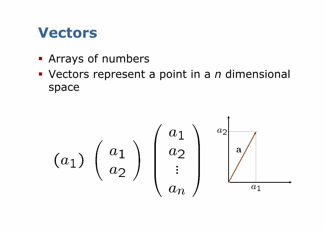
Vectors
§ Arrays of numbers § Vectors represent a point in a n dimensional
space

Vectors: Scalar Product
§ Scalar-Vector Product § Changes the length of the vector, but not
its direction

Vectors: Sum
§ Sum of vectors (is commutative)
§ Can be visualized as “chaining” the vectors.

Vectors: Dot Product
§ Inner product of vectors (is a scalar)
§ If one of the two vectors, e.g. , has , the inner product returns the length of the projection of along the direction of
§ If , the two vectors are orthogonal

§ A vector is linearly dependent from if
§ In other words, if can be obtained by summing up the properly scaled
§ If there exist no such that then is independent from
Vectors: Linear (In)Dependence

§ A vector is linearly dependent from if
§ In other words, if can be obtained by summing up the properly scaled
§ If there exist no such that then is independent from
Vectors: Linear (In)Dependence

Matrices
§ A matrix is written as a table of values
§ 1st index refers to the row § 2nd index refers to the column § Note: a d-dimensional vector is equivalent
to a dx1 matrix
columns rows

Matrices as Collections of Vectors
§ Column vectors

Matrices as Collections of Vectors
§ Row vectors

Important Matrices Operations
§ Multiplication by a scalar § Sum (commutative, associative) § Multiplication by a vector § Product (not commutative) § Inversion (square, full rank) § Transposition

Scalar Multiplication & Sum
§ In the scalar multiplication, every element of the vector or matrix is multiplied with the scalar
§ The sum of two vectors is a vector consisting of the pair-wise sums of the individual entries
§ The sum of two matrices is a matrix consisting of the pair-wise sums of the individual entries

Matrix Vector Product
§ The ith component of is the dot product .
§ The vector is linearly dependent from with coefficients
column vectors row vectors

Matrix Vector Product
§ If the column vectors of represent a reference system, the product computes the global transformation of the vector according to
column vectors
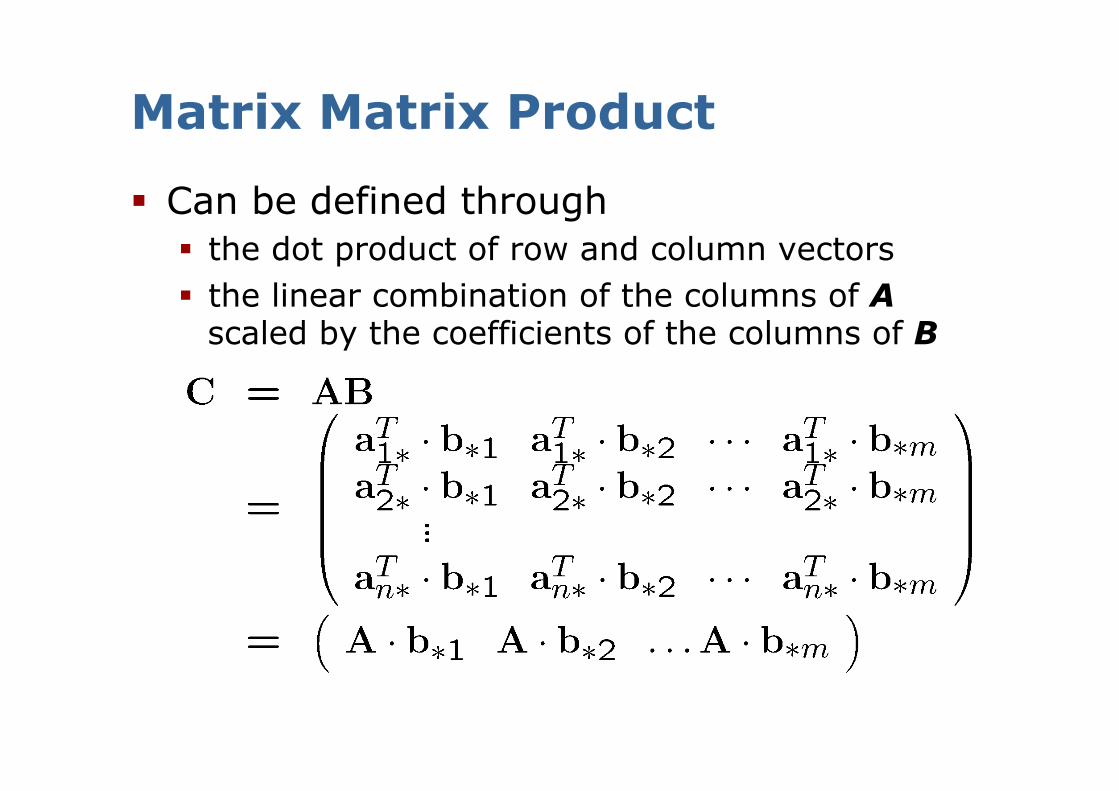
Matrix Matrix Product
§ Can be defined through § the dot product of row and column vectors § the linear combination of the columns of A
scaled by the coefficients of the columns of B

Matrix Matrix Product
§ If we consider the second interpretation, we see that the columns of C are the “global transformations” of the columns of B through A
§ All the interpretations made for the matrix vector product hold

Linear Systems (1)
Interpretations: § A set of linear equations § A way to find the coordinates x in the
reference system of A such that b is the result of the transformation of Ax
§ Solvable by Gaussian elimination (as taught in school)

Linear Systems (2)
Notes: § Many efficient solvers exit, e.g., conjugate
gradients, sparse Cholesky decomposition § One can obtain a reduced system (A’, b’) by
considering the matrix (A, b) and suppressing all the rows which are linearly dependent
§ Let A'x=b' the reduced system with A':n'xm and b':n'x1 and rank A' = min(n',m)
§ The system might be either over-constrained (n’>m) or under-constrained (n’<m)
columns rows

Over-Constrained Systems § “More (indep) equations than variables” § An over-constrained system does not
admit an exact solution § However, if rank A’ = cols(A) one may
find a minimum norm solution by closed form pseudo inversion
Note: rank = Maximum number of linearly independent rows/columns

Under-Constrained Systems
§ “More variables than (indep) equations” § The system is under-constrained if the
number of linearly independent rows (or columns) of A’ is smaller than the dimension of b’
§ An under-constrained system admits infinite solutions
§ The degree of these infinite solutions is cols(A’) - rows(A’)

Inverse
§ If A is a square matrix of full rank, then there is a unique matrix B=A-1 such that AB=I holds
§ The ith row of A is and the jth column of A-1
are: § orthogonal (if i ≠ j) § or their dot product is 1 (if i = j)

Matrix Inversion
§ The ith column of A-1 can be found by solving the following linear system:
This is the ith column of the identity matrix

§ Only defined for square matrices § Sum of the elements on the main diagonal, that is
§ It is a linear operator with the following properties § Additivity: § Homogeneity: § Pairwise commutative:
§ Trace is similarity invariant
§ Trace is transpose invariant
§ Given two vectors a and b, tr(aT b)=tr(a bT)
Trace (tr)
b l a

§ Maximum number of linearly independent rows (columns) § Dimension of the image of the transformation
§ When is we have § and the equality holds iff is the null matrix § § is injective iff § is surjective iff § if , is bijective and is invertible iff
§ Computation of the rank is done by § Gaussian elimination on the matrix § Counting the number of non-zero rows
Rank
b l a

§ Only defined for square matrices § The inverse of exists if and only if § For matrices:
Let and , then § For matrices the Sarrus rule holds:
Determinant (det)

§ For general matrices?
Let be the submatrix obtained from by deleting the i-th row and the j-th column
Rewrite determinant for matrices:
Determinant

§ For general matrices?
Let be the (i,j)-cofactor, then This is called the cofactor expansion across the first row
Determinant

§ Problem: Take a 25 x 25 matrix (which is considered small). The cofactor expansion method requires n! multiplications. For n = 25, this is 1.5 x 10^25 multiplications for which a today supercomputer would take 500,000 years.
§ There are much faster methods, namely using Gauss
elimination to bring the matrix into triangular form.
Because for triangular matrices the determinant is the product of diagonal elements
Determinant
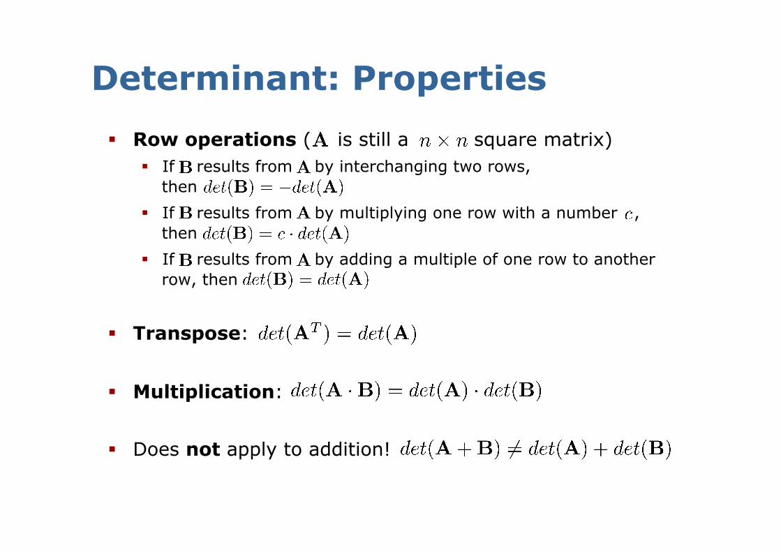
Determinant: Properties § Row operations ( is still a square matrix)
§ If results from by interchanging two rows, then
§ If results from by multiplying one row with a number , then
§ If results from by adding a multiple of one row to another row, then
§ Transpose:
§ Multiplication:
§ Does not apply to addition!

Determinant: Applications § Find the inverse using Cramer’s rule
with being the adjugate of
with Cij being the cofactors of A, i.e.,

Determinant: Applications § Find the inverse using Cramer’s rule
with being the adjugate of § Compute Eigenvalues:
Solve the characteristic polynomial § Area and Volume:
( is i-th row)

§ A matrix is orthonormal iff its column (row) vectors represent an orthonormal basis
§ As linear transformation, it is norm preserving
§ Some properties: § The transpose is the inverse § Determinant has unity norm (± 1)
Orthonormal Matrix

§ A Rotation matrix is an orthonormal matrix with det =+1 § 2D Rotations
§ 3D Rotations along the main axes
§ IMPORTANT: Rotations are not commutative
Rotation Matrix

Matrices to Represent Affine Transformations § A general and easy way to describe a 3D
transformation is via matrices
§ Takes naturally into account the non-commutativity of the transformations
§ See: homogeneous coordinates
Rotation Matrix
Translation Vector

Combining Transformations § A simple interpretation: chaining of transformations
(represented as homogeneous matrices) § Matrix A represents the pose of a robot in the space § Matrix B represents the position of a sensor on the robot § The sensor perceives an object at a given location p, in
its own frame [the sensor has no clue on where it is in the world]
§ Where is the object in the global frame?
p

Combining Transformations § A simple interpretation: chaining of transformations
(represented as homogeneous matrices) § Matrix A represents the pose of a robot in the space § Matrix B represents the position of a sensor on the robot § The sensor perceives an object at a given location p, in
its own frame [the sensor has no clue on where it is in the world]
§ Where is the object in the global frame?
B
Bp gives the pose of the object wrt the robot

Combining Transformations § A simple interpretation: chaining of transformations
(represented as homogeneous matrices) § Matrix A represents the pose of a robot in the space § Matrix B represents the position of a sensor on the robot § The sensor perceives an object at a given location p, in
its own frame [the sensor has no clue on where it is in the world]
§ Where is the object in the global frame? B
Bp gives the pose of the object wrt the robot
ABp gives the pose of the object wrt the world
A

§ A matrix is symmetric if , e.g.
§ A matrix is skew-symmetric if , e.g.
§ Every symmetric matrix: § is diagonalizable , where is a diagonal matrix
of eigenvalues and is an orthogonal matrix whose columns are the eigenvectors of
§ define a quadratic form
Symmetric Matrix
b l a

§ The analogous of positive number
§ Definition
§ Example
§
Positive Definite Matrix

§ Properties § Invertible, with positive definite inverse § All real eigenvalues > 0 § Trace is > 0 § Cholesky decomposition
Positive Definite Matrix

Jacobian Matrix
§ It is a non-square matrix in general
§ Given a vector-valued function
§ Then, the Jacobian matrix is defined as

§ It is the orientation of the tangent plane to the vector-valued function at a given point
§ Generalizes the gradient of a scalar valued function
Jacobian Matrix

Quadratic Forms
§ Many functions can be locally approximated with quadratic form
§ Often, one is interested in finding the minimum (or maximum) of a quadratic form, i.e.,

Quadratic Forms
§ Question: How to efficiently compute a solution to this minimization problem
§ At the minimum, we have § By using the definition of matrix product,
we can compute f’

Quadratic Forms
§ The minimum of is where its derivative is 0
§ Thus, we can solve the system
§ If the matrix is symmetric, the system becomes
§ Solving that, leads to the minimum

Further Reading
§ A “quick and dirty” guide to matrices is the Matrix Cookbook available at: http://matrixcookbook.com