common risk factors in the returns on stocks and bonds* · not explained by other factors. (b) the...

Journal of Financial Economics 33 (1993) 3-56. North-Holland

Common risk factors in the returns on stocks and bonds*

Eugene F. Fama and Kenneth R. French Unirrrsit.v 01 Chicayo. Chiccup. I .L 60637, C;S;L

Received July 1992. final version received September 1992

This paper identities five common risk factors in the returns on stocks and bonds. There are three stock-market factors: an overall market factor and factors related to firm size and book-to-market equity. There are two bond-market factors. related to maturity and default risks. Stock returns have shared variation due to the stock-market factors, and they are linked to bond returns through shared variation in the bond-market factors. Except for low-grade corporates. the bond-market factors capture the common variation in bond returns. Most important. the five factors seem to explain average returns on stocks and bonds.

1. Introduction

The cross-section of average returns on U.S. common stocks shows little relation to either the market /Is of the Sharpe (1964tLintner (1965) asset- pricing model or the consumption ps of the intertemporal asset-pricing model of Breeden (1979) and others. [See, for example, Reinganum (198 1) and Breeden, Gibbons, and Litzenberger (1989).] On the other hand, variables that have no special standing in asset-pricing theory show reliable power to explain the cross-section of average returns. The list of empirically determined average- return variables includes size (ME, stock price times number of shares), leverage, earnings/price (E/P), and book-to-market equity (the ratio of the book value of a firm’s common stock, BE, to its market value, ME). [See Banz (1981). Bhandari (1988). Basu (1983). and Rosenberg, Reid, and Lanstein (19853.1

Correspondence to: Eugene F. Fama. Graduate School of Business. University of Chicago, 1101 East 58th Street. Chicago. IL 60637, USA.

*The comments of David Booth, John Cochrane. Sai-fu Chen, Wayne Ferson. Josef Lakonishok. Mark Mitchell, G. William Schwert. Jay Shanken. and Rex Sinquefield are gratefully acknowledged. This research is supported by the National Science Foundation (Fama) and the Center for Research in Securities Prices (French).

030%405X.93.S05.00 C 1993-Elsevier Science Publishers B.V. Ail rights reserved

4 E.F. Fuma and K.R. French. Common risk f&run in r~ock and bond remrns

Fama and French (1992a) study the joint roles of market 8, size, E;P, leverage, and book-to-market equity in the cross-section of average stock returns. They find that used alone or in combination with other variables, /I (the slope in the regression of a stock’s return on a market return) has little information about average returns. Used alone, size, E/P, leverage, and book-to-market equity have explanatory power. In combinations, size (ME) and book-to-market equity (BE/ME) seem to absorb the apparent roles of leverage and E;‘P in average returns. The bottom-line result is that two empirically determined variables, size and book-to-market equity, do a good job explaining the cross-section of average returns on NYSE, Amex, and NASDAQ stocks for the 1963-1990 period.

This paper extends the asset-pricing tests in Fama and French (1992a) in three ways. (a) We expand the set of asset returns to be explained. The only assets con-

sidered in Fama and French (1992a) are common stocks. If markets are integrated, a single model should also explain bond returns. The tests here include U.S. government and corporate bonds as well as stocks.

(b) We also expand the set of variables used to explain returns. The size and book-to-market variables in Fama and French (1992a) are directed at stocks. We extend the list to term-structure variables that are likely to play a role in bond returns. The goal is to examine whether variables that are important in bond returns help to explain stock returns, and vice versa. The notion is that if markets are integrated, there is probably some overlap between the return processes for bonds and stocks.

(c) Perhaps most important, the approach to testing asset-pricing models is different. Fama and French (1992a) use the cross-section regressions of Fama and MacBeth (1973): the cross-section of stock returns is regressed on variables hypothesized to explain average returns. It would be difficult to add bonds to the cross-section regressions since explanatory variables like size and book-to-market equity have no obvious meaning for government and corporate bonds.

This paper uses the time-series regression approach of Black, Jensen, and Scholes (1972). Monthly returns on stocks and bonds are regressed on the returns to a market portfolio of stocks and mimicking portfolios for size, book-to-market equity (BE/‘ME), and term-structure risk factors in returns. The time-series regression slopes are factor loadings that, unlike size or BE/ME, have a clear interpretation as risk-factor sensitivities for bonds as well as for stocks.

The time-series regressions are also convenient for studying two important asset-pricing issues.

(a) One of our central themes is that if assets are priced rationally, variables that are related to average returns, such as size and book-to-market equity, must proxy for sensitivity to common (shared and thus undiversiliable) risk factors in

E.F. Famu und K.R. French. Common risk factors in stock and bond returns 5

returns. The time-series regressions give direct evidence on this issue. In particular, the slopes and R’ values show whether mimicking portfolios for risk factors related to size and BE/lVCIE capture shared variation in stock and bond returns not explained by other factors.

(b) The time-series regressions use excess returns (monthly stock or bond returns minus the one-month Treasury bill rate) as dependent variables and either excess returns or returns on zero-investment portfolios as explanatory variables. In such regressions, a well-specified asset-pricing model produces intercepts that are indistinguishable from 0 [Merton (1973)J The estimated intercepts provide a simple return metric and a formal test of how well different combinations of the common factors capture the cross-section of average returns. Moreover, judging asset-pricing models on the basis of the intercepts in excess-return regressions imposes a stringent standard. Competing models are asked to explain the one-month bill rate as well as the returns on longer-term bonds and stocks.

Our main results are easy to summarize. For stocks, portfolios constructed to mimic risk factors related to size and BE/ME capture strong common variation in returns, no matter what else is in the time-series regressions. This is evidence that size and book-to-market equity indeed proxy for sensitivity to common risk factors in stock returns. Moreover, for the stock portfolios we examine, the intercepts from three-factor regressions that include the excess market return and the mimicking returns for size and BE/ME factors are close to 0. Thus a market factor and our proxies for the risk factors related to size and book- to-market equity seem to do a good job explaining the cross-section of average stock returns.

The interpretation of the time-series regressions for stocks is interesting. Like the cross-section regressions of Fama and French (1992a), the time-series regressions say that the size and book-to-market factors can explain the differences in average returns across stocks. But these factors alone cannot explain the large difference between the average returns on stocks and one-month bills. This job is left to the market factor. In regressions that also include the size and book- to-market factors, all our stock portfolios produce slopes on the market factor that are close to 1. The risk premium for the market factor then links the average returns on stocks and bills.

For bonds, the mimicking portfolios for the two term-structure factors (a term premium and a default premium) capture most of the variation in the returns on our government and corporate bond portfolios. The term-structure factors also ‘explain’ the average returns on bonds, but the average premiums for the term-structure factors, like the average excess bond returns, are close to 0. Thus, the hypothesis that all the corporate and government bond portfolios have the same long-term expected returns also cannot be rejected.

The common variation in stock returns is largely captured by three stock- portfolio returns, and the common variation in bond returns is largely explained

by two bond-portfolio returns. The stock and bond markets. however, are far from stochastically segmented. Used alone in the time-series regressions. the term-structure factors capture strong variation in stock returns; indeed, the slopes on the term-structure factors in the regressions for stocks are much like those for bonds. But interestingly. when stock-market factors are also included in the regressions, all of our stock portfolios load in about the same way on the two term-structure factors and on the market factor in returns. As a result, a market portfolio of stocks captures the common variation in stock returns associated with the market factor and the two term-structure factors.

The stochastic links between the bond and stock markets do. however. seem to come largely from the term-structure factors. Used alone. the excess market return and the mimicking returns for the size and book-to-market equity factors seem to capture common variation in bond returns. But when the two term- structure factors are included in the bond regressions, the explanatory power of the stock-market factors disappears for all but the low-grade corporate bonds.

In a nutshell, our results suggest that there are at least three stock-market factors and two term-structure factors in returns. Stock returns have shared variation due to the three stock-market factors, and they are linked to bond returns through shared variation in the two term-structure factors. Except for low-grade corporate bonds, only the two term-structure factors seem to produce common variation in the returns on government and corporate bonds.

The story proceeds as follows. We first introduce the inputs to the time-series regressions: the explanatory variables and the returns to be explained (sections Z and 3). We then use the regressions to attack our two central asset-pricing issues: how do different combinations of variables capture (a) the common variation through time in the returns on bonds and stocks (section 4) and (b) the cross-section of average returns (section 5).

2. The inputs to the time-series regressions

The explanatory variables in the time-series regressions include the returns on a market portfolio of stocks and mimicking portfolios for the size. book- to-market, and term-structure factors in returns. The returns to be explained are for government bond portfolios in two maturity ranges, corporate bond portfolios in five rating groups, and 25 stock portfolios formed on the basis of size and book-to-market equity.

The explanatory variables fall into two sets, those likely to be important for capturing variation in bond returns and those likely to be important for stocks. Segmenting the explanatory variables in this way sets up interesting tests of

whether factors important in stock returns help to explain bond returns and vice versa.

2.1 .I. Bond-mnrket factors

One common risk in bond returns arises from unexpected changes in interest rates. Our proxy for this factor, TERM, is the difference between the monthly long-term government bond return (from Ibbotson Associates) and the one- month Treasury bill rate measured at the end of the previous month (from the Center for Research in Security Prices, CRSP). The bill rate is meant to proxy for the general level of expected returns on bonds. so that TERM proxies for the deviation of long-term bond returns from expected returns due to shifts in interest rates.

For corporate bonds. shifts in economic conditions that change the likelihood of default give rise to another common factor in returns. Our proxy for this default factor, DEF, is the difference between the return on a market portfolio of long-term corporate bonds (the Composite portfolio on the corporate bond module of Ibbotson Associates) and the long-term government bond return.

Chen. Roll, and Ross (1986) use TERM and a variable like DEF to help explain the cross-section of average returns on NYSE stocks. They use the Fama and MacBeth (1973) cross-section regression approach: the cross-section of average stock returns is explained with the cross-section of slopes from time- series regressions of returns on TERM, a default factor, and other factors. In their tests. the default factor is the most powerful factor in average.stock returns. and TER.Cl sometimes has power. We confirm that the tracks of TER,LI and DEF show up clearly in the time-series variation of stock returns. We also find that the two variables dominate the common variation in government and corporate bond returns. In contrast to the cross-section regressions of Chen. Roll, and Ross, however, our time-series regressions say that the average premiums for DEF and TERM risks are too small to explain much variation in the cross-section of average stock returns. [Shanken and Weinstein (1990) make a similar point.]

2.1.2. Stock-market fuctors

Motiuztion - Although size and book-to-market equity seem like ad hoc variables for explaining average stock returns, we have reason to expect that they proxy for common risk factors in returns. In Fama and French (1992b) we document that size and book-to-market equity are related to economic fundamentals. Not surprisingly, firms that have high BE/ME (a low stock price relative to book value) tend to have low earnings on assets, and the low earnings persist for at least five years before and five years after book-to-market equity is

measured. Conversely. low BE. .CfE (a high stock price relative to book value) is associated with persistently high earnings.

Size is also related to profitability. Controlling for book-to-market equity, small firms tend to have lower earnings on assets than big firms. The size effect in earnings, however, is largely due to the 1980s. Until 1981. controlling for BE;.LfE, small firms are only slightly less profitable than big firms. But for small firms, the 198G1982 recession turns into a prolonged earnings depression. For some reason, small firms do not participate in the economic boom of the middle and late 1980s.

The fact that small firms can suffer a long earnings depression that bypasses big firms suggests that size is associated with a common risk factor that might explain the negative relation between size and average return. Similarly. the relation between book-to-market equity and earnings suggests that relative profitability is the source of a common risk factor in returns that might explain the positive relation between BE:.CfE and average return. Measuring the common variation in returns associated with size and BE,hfE is a major task of this paper.

The Buikfiny Blocks - To study economic fundamentals, Fama and French (1992b) use six portfolios formed from sorts of stocks on .LfE and BE ‘IlIE. We use the same six portfolios here to form portfolios meant to mimic the underlying risk factors in returns related to size and book-to-market equity. This ensures a correspondence between the study of common risk factors in returns carried out here and our complementary study of economic fundamentals.

In June of each year t from 1963 to 1991, all NYSE stocks on CRSP are ranked on size (price times shares). The median NYSE size is then used to split NYSE, Amex. and (after 1972) NASDAQ stocks into two groups. small and big (S and B). Most Amex and NASDAQ stocks are smaller than the NYSE median, so the small group contains a disproportionate number of stocks 13,616 out of 4,797 in 1991). Despite its large number of stocks, the small group contains far less than half (about 8% in 1991) of the combined value of the two size groups.

We also break NYSE, Amex, and NASDAQ stocks into three book-to- market equity groups based on the breakpoints for the bottom 30% (Lo\c), middle 40% (LCfediurn). and top 30% (High) of the ranked values of BE’.\fE for NYSE stocks. We define book common equity, BE. as the COMPUSTAT book value of stockholders’ equity, plus balance-sheet deferred taxes and investment tax credit (if available), minus the book value of preferred stock. Depending on availability, we use the redemption, liquidation, or par value (in that order) to estimate the value of preferred stock. Book-to-market equity, BE,‘,CfE. is then book common equity for the fiscal year ending in calendar year t - 1, divided by market equity at the end of December oft - 1. We do not use negative-BE firms, which are rare before 1980, when calculating the breakpoints for BE) .bfE or when forming the size-BE$.LfE portfolios. Also. only firms with ordinary

E.F. Fama und K.R. Fwnch. Common rusk /Lcrorr in srock and bond renum 9

common equity (as classified by CRSP) are included in the tests. This means that ADRs, REITs, and units of beneficial interest are excluded.

Our decision to sort firms into three groups on BE,‘ICI E and only two on ME follows the evidence in Fama and French (1992a) that book-to-market equity has a stronger role in average stock returns than size. The splits are arbitrary, however, and we have not searched over alternatives. The hope is that the tests here and in Fama and French (1992b) are not sensitive to these choices. We see no reason to argue that they are.

We construct six portfolios (S/L, S;,V, S,!H. B,‘L, B,!M, B/H) from the intersections of the two ,bfE and the three BE!hfE groups. For example. the S/L portfolio contains the stocks in the small-%fE group that are also in the low-BE/ME group, and the BI’H portfolio contains the big-.CIE stocks that also have high BE,MEs. Monthly value-weighted returns on the six portfolios are calculated from July of year t to June oft + 1. and the portfolios are reformed in June of t + 1. We calculate returns beginning in July of year t to be sure that book equity for year c - 1 is known.

To be included in the tests, a firm must have CRSP stock prices for December of year t - 1 and June of t and COMPUSTAT book common equity for year t - 1. Moreover, to avoid the survival bias inherent in the way COMPUSTAT adds firms to its tapes [Banz and Breen (1986)], we do not include firms until they have appeared on COMPUSTAT for two years. (COMPUSTAT says it rarely includes more than two years of historical data when it adds firms).

Size- Our portfolio S,LfB (small minus big), meant to mimic the risk factor in returns related to size, is the difference, each month, between the simple average of the returns on the three small-stock portfolios (SjL, S/.Cf, and S,,H) and the simple average of the returns on the three big-stock portfolios (B; L. B/&f, and B/H). Thus, ShfB is the difference between the returns on small- and big-stock portfolios with about the same weighted-average book-to-market equity. This difference should be largely free of the influence of BE/ME, focusing instead on the different return behaviors of small and big stocks.

BE//LIE - The portfolio HhfL (high minus low). meant to mimic the risk factor in returns related to book-to-market equity, is defined similarly. HML is the difference, each month, between the simple average of the returns on the two high-BE/ME portfolios (S,‘H and B/H) and the average of the returns on the two low- BE/ME portfolios (S;L and B/L). The two components of H,tlL are returns on high- and low-BE,‘&fE portfolios with about the same weighted-average size. Thus the difference between the two returns should be largely free of the size factor in returns, focusing instead on the different return behaviors of high- and low-BEllME firms. As testimony to the success of this simple procedure, the correlation between the 1963-1991 monthly mimicking returns for the size and book-to-market factors is only - 0.08.

True mimicking portfolios for the common risk factors in returns minimize the variance of firm-specific factors. The six size-BEilV E portfolios in S&fB and

H,CfL are value-weighted. Using value-weighted components is in the spirit of minimizing variance, since return vririances are negatively related to size (table 1. below). More important, using value-weighted components results in mimicking portfolios that capture the different return behaviors of small and big stocks. or high- and low-BEl.VE stocks, in a way that corresponds to realistic investment opportunities.

Market - Finally. our proxy for the market factor in stock returns is the excess market return, R.M-RF. R&l is the return on the value-weighted portfolio of the stocks in the six size-BE’ME portfolios, plus the negative-BE stocks excluded from the portfolios. RF is the one-month bill rate.

22. The returns to he espkuiwd

Bonds -The set of dependent variables used in the time-series regressions includes the excess returns on two government and five corporate bond portfolios. The government bond portfolios (from CRSP) cover maturities from 1 to 5 years and 6 to 10 years. The five corporate bond portfolios, for Moody’s rating groups Aaa, Aa. A, Baa. and LG (low-grade, that is, below Baa) are from the corporate bond module of Ibbotson Associates (provided to us by Dimensional Fund Advisors).

Stocks - For stocks. we use excess returns on 25 poitfolios, formed on size and book-to-market equity. as dependent variables in the time-series regressions. We use portfolios formed on size and BE/ME because we seek to determine whether the mimicking portfolios SMB and HAIL capture common factors in stock returns related to size and book-to-market equity. Portfolios formed on size and BE.‘AIE will also produce a wide range of average returns to be explained by competing asset-pricing equations [Fama and French (1992a)]. Later, however, we use portfolios formed on E.P (earnings/price) and DiP (dividend/price). variables that are also informative about average returns [e.g.. Keim (1988)], to check the robustness of our results on the ability of our explanatory factors to capture the cross-section of average returns.

The 25 size-BE,‘,LfE portfolios are formed much like the six size-BE;&LIE portfolios discussed earlier. In June of each year t we sort NYSE stocks by size and (independently) by book-to-market equity. For the size sort. .LIE is measured at the end of June. For the book-to-market sort, ME is market equity at the end of December of c - 1. and BE is book common equity for the fiscal year ending in calendar year r - 1. We use NYSE breakpoints for ME and BE;.tfE to allocate NYSE. Amex. and (after 1972) NASDAQ stocks to five size quintiles and five book-to-market quintiles. We construct 25 portfolios from the intersections of the size and BE, ,LfE quintiles and calculate value-weighted monthly returns on the portfolios from July off to June of r + 1. The excess returns on these 25 portfolios for July 1963 to December 1991 are the dependent variables for stocks in the time-series regressions.

E.F. Fumo and R.R. French, Commor? rtsk /actors in srock und bond rerurns I1

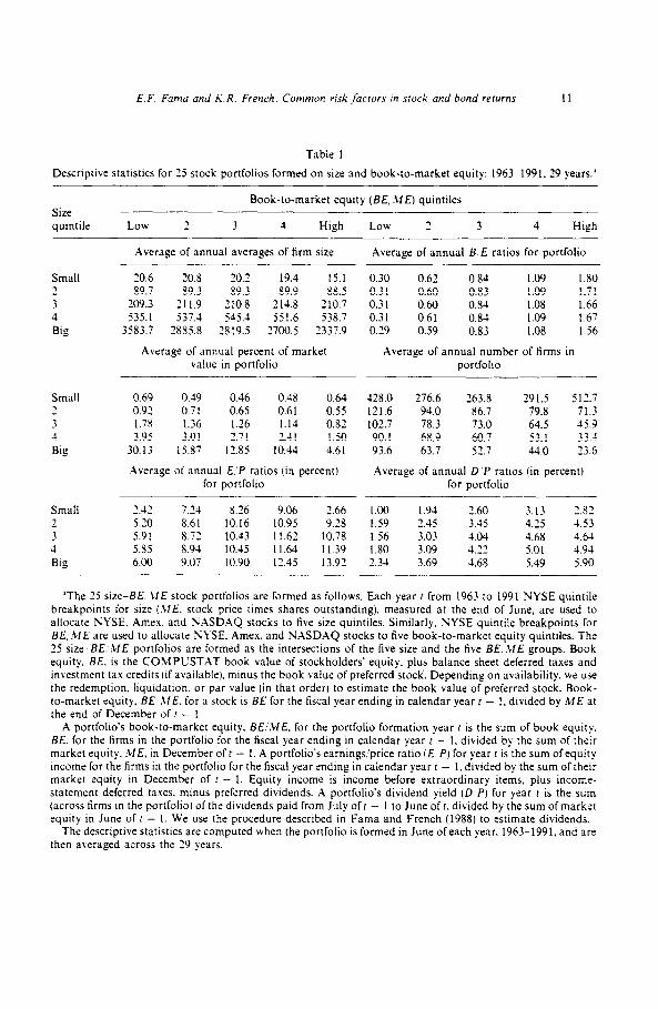
Table I

Descriptive statistics for 25 stock portfolios formed on size and book-to-market equity: 1963-1991. 29 years.’

Book-to-market equity (BE, ME) quintiies Size quintile Low 1 3 4 High Low z 3 4 High

Small 2 3 4 Big

Small

4

Big

Small 1

; 4 Big

Average of annual averages of firm size Average of annual 8. E ratios for portfolio

20.6 20.8 _ ‘0 ._ ’ 19.4 15.1 0.30 0.62 0.84 1.09 1.80 89.7 89.3 89.3 89.9 88.5 0.31 0.60 0.83 1.09 1.71

209.3 211.9 210.8 214.8 210.7 0.31 0.60 0.84 1.08 1.66 535.1 537.4 545.4 551.6 538.7 0.31 0.6 1 0.84 1.09 1.67

3583.7 2885.8 2819.5 2700.5 1337.9 0.29 0.59 0.83 1.08 1.56

Average of annual percent of market Average of annual number of firms in value in portfolio portfolio

0.69 0.49 0.46 0.48 0.64 428.0 276.6 263.8 191.5 512.7 0.92 0.71 0.65 0.6 I 0.55 121.6 94.0 86.7 79.8 71.3 1.78 1.36 1.26 1.14 0.82 102.7 78.3 73.0 64.5 45.9 3.95 3.01 2.71 2.4 I 1.50 90. I 68.9 60.7 53.1 33.4

30.13 15.87 12.85 10.44 4.61 93.6 63.7 51.7 44.0 23.6

Average of annual E’P ratios (in percent) Average of annual D’P ratios (in percent) for portfolio for portfolio

2.42 7.24 8.26 9.06 2.66 1.00 I .94 2.60 3.13 2.82

5.20 5.91 8.61 8.73 10.16 10.43 10.95 Il.61 10.78 9.28 l.59 1.56 2.45 3.03 4.04 3.45 4.25 4.68 4.53 4.64 5.85 8.94 10.45 11.64 11.39 1.80 3.09 4.22 5.01 4.94 6.00 9.07 10.90 12.45 13.92 2.34 3.69 4.68 5.49 5.90

“The 25 size-BE. ME stock portfolios are formed as follows. Each year t from 1963 to 1991 NYSE quinttle breakpoints for size (.UE. stock price times shares outstanding), measured at the end of June, are used to allocate NYSE. Amex. and NASDAQ stocks to five size quintiles. Similarly, NYSE quintile breakpoints for BE, ME are used to allocate NYSE. Amex. and NASDAQ stocks to five book-to-market equity quintiles. The 25 size-BE,‘.LIE portfolios are formed as the intersections of the five size and the five BE. ME groups. Book equity. BE. is the COMPUSTAT book value of stockholders’ equity, plus balance sheet deferred taxes and investment tax credits lif available). minus the book value of preferred stock. Depending on avjailability. we use the redemption. liquidation. or par value (in that order) to estimate the book value of preferred stock. Book- to-market equity. BE .ME. for a stock is BE for the fiscal year ending in calendar year r - 1. divided by ME at the end of December oft - 1.

A portfolio’s book-to-market equity, BE,‘XfE. for the portfolio formation year c is the sum of book equity. BE. for the firms in the portfolio for the fiscal year endmg in calendar year t - I, divided by the sum of their market equity. ME, in December oft - I. A portfolio’s earnings/price ratio (E P) for year I is the sum ofequity income for the firms in the portfolio for the fiscal year ending in calendar year t - 1. divided by the sum of their market equity in December of r - 1. Equity income is income before extraordinary items, plus income- statement deferred taxes. minus preferred dividends. A portfolio’s dividend yield (D P) for year t is the sum (across firms in the portfolio) of the dividends paid from July oft - 1 to June of r. divided by the sum of market equity in June oft - I. We use the procedure described in Fama and French (1988) to estimate dividends.

The descriptive statistics are computed when the portfolio is formed in June ofeach year. 1963-1991, and are then averaged across the 29 years.

12 E.F. Fama und K. R. French. Common risk /&tom in stock md bond returns

Table 1 shows that, because we use NYSE breakpoints to form the 25 size-BE, ,CIE portfolios, the portfolios in the smallest size quintile have the most stocks (mostly small Amex and NASDAQ stocks). Although they contain many stocks, each of the five portfolios in the smallest size quintile is on average less than 0.70% of the combined value of stocks in the 25 portfolios. In contrast, the portfolios in the largest size quintile have the fewest stocks but the largest fractions of value. Together, the five portfolios in the largest JIE quintile average about 74% of total value. The portfolio of stocks in both the largest size and lowest BE/ME quintiles (big successful firms) alone accounts for more than 30% of the combined value of the 25 portfolios. And note that using all stocks, rather than just NYSE stocks, to define the size quintiles would result in an even more skewed distribution of value toward the biggest size quintile.

Table 1 also shows that in every size quintile but the smallest, both the number of stocks and the proportion of total value accounted for by a portfolio decrease from lower- to higher-BE/ME portfolios. This pattern has two causes. First, using independent size and book-to-market sorts of NYSE stocks to form portfolios means that the highest-BE/ME quintile is tilted toward the smallest stocks. Second, Amex and NASDAQ stocks, mostly small, tend to have lower book-to-market equity ratios than NYSE stocks of similar size. In other words, NYSE stocks that are small in terms of ME are more likely to be fallen angels (big firms with low stock prices) than small Amex and NASDAQ stocks.

3. The playing field

Table 2 summarizes the dependent and explanatory returns in the time-series regressions. The average excess returns on the portfolios that serve as dependent variables give perspective on the range of average returns that competing sets of risk factors must explain. The average returns on the explanatory portfolios are the average premiums per unit of risk (regression slope) for the candidate common risk factors in returns.

3.1. The dependent retwxs

Stocks - The 25 stock portfolios formed on size and book-to-market equity produce a wide range of average excess returns, from 0.32% to 1.05% per month. The portfolios also confirm the Fama-French (1992a) evidence that there is a negative relation between size and average return, and there is a stronger positive relation between average return and book-to-market equity. In all but the lowest-BE/ME quintile, average returns tend to decrease from the small- to the big-size portfolios. The relation between average return and book-to-market equity is more consistent. In every size quintile, average returns tend to increase with BE/:bfE, and the differences between the average returns

E.F. Fame und K. R. French. Common risk fk!ors m slack and bond rerurm 13

for the highest- and lowest-BE;‘.CJE portfolios range from 0.19% to 0.62% per

month. Our time-series regressions attempt to explain the cross-section of average

returns with the premiums for the common risk factors in returns. The wide range of average returns on the 25 stock portfolios, and the size and book- to-market effects in average returns, present interesting challenges for competing sets of risk factors.

Most of the ten portfolios in the bottom two BEI’ME quintiles produce average excess returns that are less than two standard errors from 0. This is an example of a well-known problem [Merton (1980)] : because stock returns have high standard deviations (around 6% per month for the size-BE ‘.CJE portfolios), large average returns often are not reliably different from 0. The high volatility of stock returns does not mean, however, that our asset-pricing tests will lack power. The common factors in returns will absorb most of the variation in stock returns, making the asset-pricing tests on the intercepts in the time- series regressions quite precise.

Borrds - In contrast to the stock portfolios, the average excess returns on the government and corporate bond portfolios in table 2 are puny. All the average excess bond returns are less than 0.15% per month, and only one of seven is more than 1.5 standard errors from 0. There is little evidence in table 2 that (a) average returns on government bonds increase with maturity, (b) long-term corporate bonds have higher average returns than government bonds, or (c) average returns on corporate bonds are higher for lower-rating groups.

The flat cross-section of average bond returns does not mean that bonds are uninteresting dependent variables in the asset-pricing tests. On the contrary. bonds are good candidates for rejecting asset-pricing equations that predict patterns in the cross-section of average returns based on different slopes on the common risk factors in returns.

3.2. The explanatory returns

In the time-series regression approach to asset-pricing tests, the average risk premiums for the common factors in returns are just the average values of the explanatory variables. The average value of RXJ-RF (the average premium per unit of market p) is 0.43% per month. This is large from an investment perspective (about 5% per year), but it is a marginal 1.76 standard errors from 0. The average S,VJB return (the average premium for the size-related factor in returns) is only 0.27% per month (t = 1.73). We shall find, however, that the slopes on SAJB for the 25 stock portfolios cover a range in excess of 1.7, so the estimated spread in expected returns due to the size factor is large, about 0.46% per month. The book-to-market factor HAIL. produces an average premium of 0.40% per month (t = 2.91), that is large in both practical and statistical terms.

i

Kill

0.

97

4.52

3.

97

0.05

-

0.05

0.

03

7‘11

0.

54

0.22

45

.97

0.94

0.

90

0.65

l.‘

i’(;

0.60

3.

03

3.66

0.

05

- 0.

w

0.00

(‘1

) 0.

62

2.24

5.

10

0.20

-

0.04

0.

04

RWRb

0.

43

4.54

I .

76

Rhl

O

OS0

3.

55

2.61

Sh

f0

0.27

2.

89

1.73

Ilh

fL

0.40

2.

54

2.9

I 7’

1:R

hl

0.06

3.

02

0.38

DE

b O

.O:!

I.60

0.2

I

0.05

-

0.04

0.

03

RII

I-R

I.’

RM

O

- 0.

10

- 0.

05

0.02

0.

78

I.00

0.19

0.

07

0.23

0.

32

- 0.

00

O.II

( 0.

06

0.07

-

0.38

-

0.00

0.

05

~ 0.

00

- 0.

00

0.34

0.

w

~ 0.

20

-- 0.

04

- 0.

00

- 0.

07

- 0.

00

ari;i

blcs

: lix

ccss

re

turn

s on

go

vern

wzn

l an

d co

rpor

vk

bond

s

I S

C;

0. I

2 6

IOG

0.

I4

AA

A

0.06

A

A

0.07

A

0.

0x

BA

A

0.14

LG

0.

I 3

Sld 1.25

2.

03

2.34

2.

23

2.25

2.

35

2.52

Aul

ocor

r. fo

r la

g

1 (tw

1)

I 2

12

Expl

anat

ory

retu

rns

Ikpe

ndzl

ll \

1.71

1.

24

0.44

0.

58

0.63

I.0

9

0. I

5 -

0.08

0.

I ?

- 0.

05

0. I6

-

0.03

0.

I9 -

0.04

0.

2 I

- 0.

03

0.2

I 0.

00

0.23

0.

05

SMII

1.00

-

0.08

-

0.07

0.

I7

0.01

0.

02

0.02

0.

03

0.04

0.

03

0.08

I .m

-

0.05

I.0

0 c

0.0x

-

0.69

c.

c-

? k 2 2 : t

De

pe

nd

en

t va

riab

les:

Ex

ce

ss

retu

rns

on

25

sto

ck

p

ort

folio

s fo

rme

d

on

ME

an

d B

E/M

E

Size

qu

intil

c

sm:1

11

2 3 4 Kg

LOW

0.39

0.44

0.43

0.

48

0.40

Bo

ok

-to

-ma

rke

t e

qu

ity

(BE/

ME)

q

uin

tile

s

~~

~

~__

__~

~

~_.

_

2 3

4 H

igh

Lo

w

2 3

4 H

igh

Me

an

s St

an

da

rd

de

via

tion

s

0.70

0.

79

0.88

1.

01

7.76

6.

84

6.29

5.

99

6.27

0.

71

0.85

0.

84

I .02

7.

28

6.42

5.

85

5.33

6.

06

0.66

0.

68

0.8

I O

.Y7

6.71

5.

71

5.27

4.

Y2

5.b

Y

0.35

0.

57

0.17

I .

05

5.97

5.

44

5.03

4.

95

5.75

0.36

0.

32

0.56

0.

59

4.95

4.

70

4.38

4.

27

4.85

t-st

atis

tics

for

me

an

s

Sn

xlll

0.93

I .8

X

2.33

2.

73

2.97

2

I.1 1

2.

05

2.6’

) 2.

9 I

3.1

I 3

I.IX

2.

12

2.39

3.

04

3.15

4 I .

49

1.19

2.

08

LXX

3.

36

I)&

I .

50

I .42

I .

34

2.43

2.

2b

‘Uhf

is

th

e v

alu

e-w

eig

hte

d

mo

nth

ly

pe

rce

nt

retu

rn

on

th

e s

toc

ks

in

the

25

size

-BE/

ME

po

rtfo

lios,

p

lus

the

ne

ga

tive

-BE

sto

ck

s e

xclu

de

d f

rom

th

e

po

rtfo

lios.

K

F is

th

e o

ne

-mo

nth

Tr

ea

sury

b

ill

rate

, o

bse

rve

d a

t th

e b

eg

inn

ing

o

f th

e m

on

th.

LTG

is

th

e l

on

g-t

erm

g

ove

rnm

en

t b

on

d r

etu

rn.

CB

is

the

retu

rn

on

ii

pro

xy

for

the

rm

lrke

t p

ort

folio

o

f lo

ng

-te

rm

co

rpo

rate

b

on

ds.

TE

RM

is

LTG

-RF.

D

EF

is C

B~

LTG

. SM

B

(sm

all

min

us

big

) is

th

e d

rlTe

ren

ce

be

twe

en

th

e r

etu

rns

on

sn

dl-

sto

ck

a

ntI

big

-sto

ck

p

ort

tidio

s w

ith

ah

ou

t th

e s

:mx

we

igh

ted

ave

rag

e h

oo

k-t

o-m

ark

et

eq

uity

. I/

Ml.

(hig

h

min

us

low

) is

th

e M

ere

nc

e

be

twe

en

th

e r

etu

rns

on

hig

h a

nd

lo

w

ho

ok

-to

-ma

rke

t e

qu

ity

po

rtfo

lios

with

a

hu

ut

the

sa

me

we

igh

ted

ave

rag

e s

ize

. R

MO

is

th

e s

um

o

f th

e i

nte

rcc

pl

an

d

resi

du

als

l&

n

lhc

re

gre

ssio

n

(I)

of

KM

-R

F on

?‘

ERM

, L)

EF,

SMB

, a

nd

IIM

L.

‘l‘h

e s

cvc

’n h

od

p

ort

lidiu

s u

sed

HIS

de

pe

nd

cn

~ v

ari;

thle

s in

th

e e

xce

ss-r

etu

rn

reg

ress

ion

s a

re I

- to

5-y

ea

r a

nd

b-

to IO

-ye

ar

go

vern

me

nts

(I

-5G

a

nd

6 ~

IW)

;IIIJ

c

orl

xnxt

e

bo

nd

s ra

ted

AX

I, A

;I, A

, Ik

lu.

an

d b

elo

w H

na

(I.(

;)

by

Mo

od

y’r.

Th

e

25 s

ize

-BE/

ME

sto

ck

p

ort

foo

lios

are

fo

rme

d

as

roo

llow

s. E

ac

h y

ea

r r f

rom

19

03 t

o

1991

NY

SE

qu

intil

e

hre

;tk

po

Lits

fo

r si

ze (

ME,

st

oc

k

pric

e t

ime

s sh

are

s o

uts

tan

din

g),

m

ea

sure

d

al

Ihe

en

d o

f Ju

ne

, a

re u

sed

lo

allo

ca

te

NY

SE.

An

~x,

a

nd

NA

SDA

Q

sto

ck

s to

liv

e s

ize

qu

intil

es.

Si

mila

rly,

NY

SE

qu

intil

e

bre

ak

po

ints

fo

r B

E/M

E a

re u

sed

to

allo

ca

te N

Y!%

, A

me

x,

an

d

NA

SDA

O

SIO

C~

S lo

liv

e h

oo

k-t

o-n

l;lrk

ct

eq

uity

q

uin

tile

s.

In

U/:

‘/M

E,

WB

is

ho

ok

com

m~m

eq

uit

y fo

r th

e l

isc

al

ye

ar

en

din

g i

n c

ale

nd

ar

ye

ar I

- I,

an

d M

L’

is l

i)r

the

c

d

ol’

De

ce

mh

cr

d

I -

I. Th

e

25 s

ix

&E/

ME

port

folios

are

h

rmd

as

the

in

ters

ecti

on

s of

the

tivc

siz

e

an

d t

he

liv

e

HE/

ME

gro

up

s.

Va

lue

-we

igh

ted

nlo

nth

ly

prr

ce

nt

retu

rns

on

th

e p

d’d

ios

are

ca

lda

d

thru

m J

uly

u

l y

ea

r I

to Ju

ne

d

I

+

I.

The average risk premiums for the term-structure factors are trivial relative to those of the stock-market factors. TER.Ll (the term premium) and DEF (the default premium) are on average 0.069/o and 0.029;b per month; both are within 0.3 standard errors of 0. Note, though, that TER,Zl and DEF are about as volatile as the stock-market returns S.LfB and H.CIL. Low average premiums will prevent TERM and DEF from explaining much cross-sectional variation in average returns, but high volatility implies that the two factors can capture substantial common variation in returns. In fact. the low means and high volatilities of TER.\/I and DEF will be advantageous for explaining bond returns. But the task of explaining the stron, 0 cross-sectional variation in average stock returns falls on the stock-market factors. RN-RF. SMB, and HML. which produce higher average premiums.

We turn now to the asset-pricing tests. In the time-series regression approach. the tests have two parts. In section 4 vve establish that the two bond-market returns, TER.tI and DEF, and the three stock-market returns, RXI-RF, SMB. and H&IL, are risk factors in the sense that they capture common (shared and thus undiversifiable) variation in stock and bond returns. In section 5 we use the intercepts from the time-series regressions to test whether the average premiums for the common risk factors in returns explain the cross-section of average returns on bonds and stocks.

4. Common variation in returns

In the time-series regressions, the slopes and R’ values are direct evidence on whether different risk factors capture common variation in bond and stock returns. We first examine separately the explanatory power of bond-market and stock-market factors. The purpose is to test for overlap between the stochastic processes for stock and bond returns. Do bond-market factors that are important in bond returns capture common variation in stock returns and vice versa? We then examine the joint explanatory power of the bond- and stock-market factors, to develop an overall story for the common variation in returns.

1. I. Bond-market fktors

Table 3 shows that, used alone as the explanatory variables in the time-series regressions, TERM and DEF capture common variation in stock and bond returns. The 25 stock portfolios produce slopes on TERM that are all more than five standard errors above 0; the smallest TER.Cf slope for the seven bond portfolios is 18 standard errors from 0. The slopes on DEF are all more than 7.8 standard errors from 0 for bonds, and more than 3.5 standard errors from 0 for stocks.

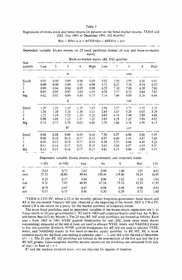
Table 3

Regressions of excess stock and bond returns (in percent) on the bond-market returns. TER.\/ and DEf: July 1963 to December 1991. 342 months.”

R(t) - RF(t) = a + mTERJf(t) + dDEF(r) -t e(t)

Dependent variable: Excess returns on 25 stock portfolios formed on size and book-to-market equity

Book-to-market equity (BE, ME) qumtiles Size quintile Low 2 3 4 High Low 2 3 -I High

Small 2 3 4 Big

Small z 3 4 Big

Small 2 3 4 Big

m r(m)

0.93 0.90 0.89 0.86 0.89 5.02 5.50 5.95 6.08 6.0 1 0.99 0.96 0.99 1.01 0.98 5.71 6.32 7.29 8.3-t 6.92 0.99 0.94 0.94 0.95 0.99 6.25 7.10 7.80 8.50 7.60 0.92 0.95 0.97 1.05 1.03 6.58 7.57 a.53 9.64 7.83 0.82 0.82 0.80 0.80 0.77 7.14 7.60 8.09 8.26 6.84

d rid) -_

1.39 1.31 1.33 1.45 1.X 3.96 4.27 4.73 5.45 5.45 1.26 1.28 1.35 1.38 1.41 3.84 4.47 5.28 6.05 5.29 1.21 1.19 I.25 1.24 1.21 4.05 4.74 5-19 5.89 4.98 0.96 1.01 1.13 1.21 1.22 3.65 1.28 5.25 5.89 4.91 0.78 0.73 0.78 0.83 0.89 3.59 3.60 4.18 4.56 4.15

R’ SW

0.06 0.08 0.09 0.10 0.10 7.50 6.57 6.00 5.68 5.95 0.08 0.10 0.13 0.17 0.12 6.97 6.09 5.45 4.87 5.69 0.10 0.12 0.15 0.17 0.14 6.38 5.35 1.86 4.48 5.2 0.11 0.14 0.17 0.21 0.15 5.63 5.04 4.57 1.39 5.31 0.13 0.15 0.16 0.17 0.12 4.61 4.33 4.00 3.89 4.55

Dependent variable: Excess returns on government and corporate bonds

I-5G 6-IOG Aaa Aa A Baa LG

m 0.45 0.72 I .02 0.99 1.00 1.01 0.81 t(m) 31.73 3880 99.94 130.44 139.80 56.24 18.05

d 0.25 0.27 0.94 0.96 I .02 1.10 1.01 t(d) 9.51 7.85 48.95 67.54 75.74 32.33 11.95

R’ 0.79 0.87 0.97 0.98 0.98 0.90 0.19 s(e) 0.57 0.75 0.41 0.30 0.29 0.72 1.80

“TERM is LTG-RF. where LX is the monthly percent long-term government bond return and RF is the one-month Treasury bill rate. observed at the beginning of the month. DEF is C&LX, where CB is the return on a proxy for the market portfolio of corporate bonds.

The seven bond portfolios used as dependent variables in the excess-return regressions are I- to S-year and 6- to lo-year governments (I-5G and GlOG) and corporate bonds rated A.aa. Aa, A. Baa, and below Baa (LG) by Moody’s, The 25 size-BE;.CfE stock portfolios are formed as follows. Each year t from 1963 to 1991 NYSE quintile breakpoints for size (.WE, stock price times shares outstanding). measured at the end of June. are used to allocate NYSE, Amex. and NASDAQ stocks to five size quintiles. Similarly, NYSE quintile breakpoints for BE’.CfE are used to allocate NYSE, Amex, and NASDAQ stocks to five book-to-market equity quintiles. In BE, ME, BE is book common equity for the fiscal year ending in calendar year f - 1, and ME is for the end of December oft - 1. The 25 size-BE, .1fE portfolios are formed as the intersections of the five size and the five BE/ME groups. Value-weighted monthly percent returns on the portfolios are calculated from July of year f to June oft + 1.

R’ and the residual standard error. s(e), are adjusted for degrees of freedom.

The slopes on TER.Cf and DEF allow direct comparisons of the common variation in stock and bond returns tracked by the term-structure variables. Interestingly. the common variation captured by TER.Cf and DEF is. if anything, stronger for stocks than for bonds. Most of the DEF slopes for stocks are bigger than those for bonds. The TER.tf slopes for stocks (all close to 1) are similar to the largest slopes produced by bonds.

As one might expect, however, the fractions of return variance explained by TER,M and DEF are higher for bonds. In the bond regression, R’ ranges from 0.49 for low-grade corporates to 0.97 and 0.98 for high-grade corporates. In contrast, R’ ranges from 0.06 to 0.21 for stocks. Thus, TERM and DEF clearly identify shared variation in stock and bond returns, but for stocks and low- grade bonds. there is plenty of variation left to be explained by stock-market factors.

There is an interesting pattern in the slopes for TER.Cl. The slopes increase from 0.45 to 0.72 for I- to S-year and 6- to lo-year governments, and then settle at values near I for four of the five long-term corporate bond portfolios. (The low-grade portfolio LG. with a slope of 0.81. is the exception.) As one would expect. long-term bonds are more sensitive than short-term bonds to the shifts in interest rates measured by TER.LI. What is striking. however, is that the 25 stock portfolios have TER.Ll slopes like those for long-term bonds. This suggests that the risk captured by TER,Cf results from shocks to discount rates that affect long-term securities. bonds and stocks, in about the same way.

There are interesting parallels between the TER,Lf slopes observed here and our earlier evidence that yield spreads predict bond and stock returns. In Fama and French (1959), kve find that a spread of long-term minus short-term bond yields (an ex ante version of TERXI) predicts stock and bond returns, and captures about the same variation through time in the expected returns on long-term bonds and stocks. We conjectured that the yield spread captures variation in a term premium for discount-rate changes that affect all long-term securities in about the same way. The similar slopes on TER,Lf for long-term bonds and stocks observed here seem consistent with that conjecture.

Our earlier work also finds that the return premium predicted by the long- term minus short-term yield spread wanders between positive and negative values, and is on average close to 0. This parallels the evidence here (table 2) that the average premium for the common risk associated with shifts in interest rates (the average value of TERM) is close to 0.

The pattern in the DEF slopes in table 3 is also interesting. The returns on small stocks are more sensitike to the risk captured by DEF than the returns on big stocks. The DEF slopes for stocks tend to be larger than those for corporate bonds, which are larger than those for governments. DEF thus seems to capture a common ‘default’ risk in returns that increases from government bonds to corporates, from bonds to stocks. and from big stocks to small stocks. Again, there is an interesting parallel between this pattern in the DEF slopes and the

E.F. Fumu und K.R. Frewh. Common risk fucrors in srocb und bond reiurns 19

similar pattern observed in Fama and French (1989) in time-series regressions of stock and bond returns on an ex ante version of DEF (a spread of low-grade minus high-grade bond yields).

Using the Fama-Macbeth (1973) cross-section regression approach and stock portfolios formed on ranked values of size, Chan, Chen. and Hsieh (1985) and Chen, Roll, and Ross (1986) find that the cross-section of slopes on a variable like DEF goes a long way toward explaining the negative relation between size and average stock returns. Given the negative relation between size and the slopes on DEF in table 3, it is easy to see why the DEf slopes work well in cross-section return regressions for size portfolios.

Our time-series regressions suggest, however, that DEF cannot explain the size effect in average stock returns. In the time-series regressions, the average premium for a unit of DEF slope is the mean of DEF, a tiny 0.02% per month. Likewise, the average TERM return is only 0.06% per month. As a result, we shall see that the intercepts in the regressions of stock returns on TERM and DEF leave strong size and book-to-market effects in average returns. We shall also find that when the stock-market factors are added to the regressions, the negative relation between size and the DEF slopes in table 3 disappears.

42. Stock-market f&ton

The role of stock-market factors in returns is developed in three steps. u’e examine (a) regressions that use the excess market return, RAGRF, to explain excess bond and stock returns, (b) regressions that use SMB and NML, the mimicking returns for the size and book-to-market factors, as explanatory variables. and (c) regressions that use RM-RF, S‘SJB. and H,VfL. The three- factor regressions work well for stocks, but the one- and two-factor regressions help explain why.

The Murket - Table 4 shows, not surprisingly, that the excess return on the market portfolio of stocks, RM-RF, captures more common variation in stock returns than the term-structure factors in table 3. For later purposes. however. the important fact is that the market leaves much variation in stock returns that might be explained by other factors. The only RZ values near 0.9 are for the big-stock low-book-to-market portfolios. For small-stock and high-BE/ME portfolios, R’ values less than 0.8 or 0.7 are the rule. These are the stock portfolios for which the size and book-to-market factors, SMB and H.LIL, will have their best shot at showing marginal explanatory power.

The market portfolio of stocks also captures common variation in bond returns. Although the market fls are much smaller for bonds than for stocks. they are 5 to 12 standard errors from 0. Consistent with intuition, /? is higher for corporate bonds than for governments and higher for low-grade than for high-grade bonds. The /I for low-grade bonds (LG) is 0.30, and R.V-RF explains a tidy 19% of the variance of the LG return.

Table 1

Regressions of excess stock and bond returns (in percent) on the excess stock-market return, R.WRF: July 1963 to December 1991. 342 months.”

R(t) - RF(t) = a + b[R.Lf(rl - RF(r)] + r(r)

_

Dependent variable: Excess returns on 25 stock portfolios formed on size and book-to-market equity

Book-to-market equity (BE .CIE quintiles Size quintile Lou 2 3 1 High Low 2 3 1 Htgh

h r(h)

Small 1.40 1.26 I.11 I .06 I .08 16.33 28.12 27.01 25.03 23.01 2 I .‘I? I.15 I.12 I .02 1.13 35.76 35.56 33.12 33.1-I 3

29.04 1.36 I.15 I.04 0.96 I .oa 12.98 42.52 37.50 35.81 31.16

1 I.24 I.14 I .03 0.95 I.10 51.67 55.IZ 46.96 37.00 32.76

Btg I .03 0.99 0.89 0.84 0.89 5 I .92 61.51 13.03 35.96 27.75

R’ s(e)

Small 0.67 0.70 0.68 0.65 0.6 I -1.46 3.76 3.55 3.56 3.92 2 0.79 0.79 0.76 0.76 0.71 3.34 2.96 2.85 2.59 ?

3.25 0.8-l 0.81 0.80 0.79 0.74 2.65 2.28 2.33 3.26 2.90

; 0.89 0.90 0.87 0.80 0.76 2.0 I 1.73 I.% 2.2 1 2.83

Big 0.89 0.91 0.54 0.79 0.69 1.66 1.35 1.73 1.95 2.69

Dependent variable: Excess returns on government and corporate bonds

I -5G 6-IOG Aaa -\a A Baa LG

h 0.08 0.13 0.19 0.20 0.21 0.21 0.30

r(h) 5.24 5.57 7.53 8.14 8.42 8.73 II.90

RJ 0.07 0.0s 0.14 0.16 0.17 0.19 0.29

s(e) I.21 1.95 2.17 2.05 2.05 2.12 2.12

‘R.W is the value-heighted monthly percent return on all the stocks in the 25 size-BE.‘IW& portfolios, plus the negative-BE stocks excluded from the 25 portfolios. RF is the one-month Treasury bill rate. observed at the beginning of the month.

The seven bond portfolios used as dependent variables in the excess-return regressions are I- to 5-vear and 6- to IO-vear eovernments (I-SC and 6-IOG) and corporate bonds rated Aaa. Aa. .A. Baa. and below Baa (LG) by Moody’s The 25 size-BE, .LfE stock portfolios are formed as follous. Each year r from 1963 to 1991 NYSE quintile breakpoints for size (,LfE. stock price times shares outstanding). measured at the end of June, are used to allocate NYSE. Amex. and NASDAQ stocks to five size quintiles. Similarly. NYSE quintile breakpoints for B&ME are used to allocate NYSE, Amex. and NASDr\Q stocks to five book-to market equity quintiles. In BE ME. BE is book common equity for the fiscal year ending in calendar year r - I, and ME is for the end of December of r - I. The 25 size-BE .UE portfolios are formed as the intersections of the five size and the five BE .LfE groups. Value-weighted monthly percent returns on the portfolios are calculated from July ofyearrtoJuneofr+l.

R’ and the residual standard error. s(e), are adjusted for degrees of freedom.

E.F. Fuma and K.R. French. Common risk factors VI s[ock and bond rerurns 21

S.LfB and H.CIL -Table 5 shows that in the absence of competition from the market portfolio. SMB and H&IL. typically capture substantial time-series variation in stock returns; 20 of the 25 R’ values are above 0.2 and eight are above 0.5. Especially for the portfolios in the larger-size quintile, however, SXfB and H~ML leave common variation in stock returns that is picked up by the market portfolio in table 4.

The Marker, S,LIB, and HML - Table 5 says that, used alone, SMB and HAIL have little power to explain bond returns. Table 6 shows that when the excess market return is also in the regressions, each of the three stock-market factors captures variation in bond returns. We shall find, however, that adding the term-structure factors to the bond regressions largely kills the explanatory power of the stock-market factors. Thus the apparent role of the stock-market factors in bond returns in table 6 probably results from covariation between the term-structure and stock-market factors.

The interesting regressions in table 6 are for stocks. Not surprisingly. the three stock-market factors capture strong common variation in stock returns. The market ps for stocks are all more than 38 standard errors from 0. With one exception, the t-statistics on the SMB slopes for stocks are greater than 4; most are greater than 10. SMB, the mimicking return for the size factor, clearly captures shared variation in stock returns that is missed by the market and by HML. Moreover, the slopes on SMB for stocks are related to size. In every book-to-market quintile, the slopes on SMB decrease monotonically from smaller- to bigger-size quintiles.

Similarly, the slopes on HML, the mimicking return for the book-to-market factor, are systematically related to BEI.Lf E. In every size quintile of stocks, the H&IL slopes increase monotonically from strong negative values for the lowest- BE,!.LIE quintile to strong positive values for the highest-BE/.LIE quintile. Except for the second BE/ME quintile, where the slopes pass from negative to positive, the HML slopes are more than five standard errors from 0. HML clearly captures shared variation in stock returns, related to book-to-market equity. that is missed by the market and by SMB.

Given the strong slopes on SMB and H&IL for stocks, it is not surprising that adding the two returns to the regressions results in large increases in R2. For stocks, the market alone produces only two (of 25) R’ values greater than 0.9 (table 4); in the three-factor regressions (table 6) RZ values greater than 0.9 are routine (21 of 25). For the five portfolios in the smallest-size quintile, R2 increases from values between 0.61 and 0.70 in table 4 to values between 0.94 and 0.97 in table 6. Even the lowest three-factor R’ for stocks, 0.83 for the portfolio in the largest-size and highest-BE!rLIE quintiles, is much larger than the 0.69 generated by the market alone.

Adding SMB and HML to the regressions has an interesting effect on the market ps for stocks. In the one-factor regressions of table 4, the p for the portfolio of stocks in the smallest-size and lowest-BE/ME quintiles is 1.40. At

Tabl

e 5

Reg

ress

ions

of

wce

ss

dock

an

d bo

nd

retu

rns

(in

perc

ent)

on

the

mim

icki

ng

retu

rns

for

the

size

(SM

B)

and

book

-lo-m

arke

t eu

uilv

(II

ML)

fa

ctor

s:

Julv

.~

. I9

63

IO D

ecem

ber

1991

, 34

2 m

onth

s.”

H(r

) -

W(r

) =

0 +

.sSM

B(r

) +

IrIfM

L(

r)

+ r(

r)

Size

qu

inlil

e

Smdl

2 3 4 B

ig

Sm;II

I 2 3 ‘I B

ig

2 3 4 Big

LWV I .Y

3 1.

52

1.28

0.

X6

0.28

- O

.Y5

-~ 1

.22

-- 1.

0’)

- I.1

1 ~

1.07

0.65

0.

5’)

0.51

0.

43

0.34

Dep

cndr

n~

varia

ble:

Ex

cess

rc

Iurn

s on

25

st

ock

podo

lios

form

ed

on

size

an

d bo

ok-to

-mar

ket

equi

ly

Boo

k-lo

-mar

ket

equi

ty

(BE/

ME)

qu

inde

s

2 3

1.73

1.

46

1.12

0.

x2

0.35

I .63

1.

35

1.05

0.

77

0.22

/I

1.5’

) I .

67

22.5

2 1.

18

1.40

17

.23

o.Y3

I.1

6 14

.43

0.12

O

.Y5

IO.1

6 0.

2Y

0.44

3.

70

_ 0.

57

~ 0.

66

- 0.

65

~ 0.

65

- 0.

65

- 0.

35

- 0.

3x

- 0.

31

- 0.

36

- 0.

42

K2

~ 0

.18

0.0

I -

Y.72

-

0.16

O

.lK)

~ 12

.25

~~ 0.

1 I

- 0.

01

- IO

.84

- 0.

1 I

~ 0.

0 I

- II.

43

~ 0.

06

0.08

-

12.4

6

0.00

0.

60

0.60

0.

SY

0.53

0.

4’)

0.42

0.

44

0.43

0.

37

0.31

0.

35

0.30

0.

24

0.18

0.

23

0.18

0.

08

0.04

0.

06

s

4 H

igh

Low

21.3

8 17

.68

I3.W

9.

64

4.3’

)

21.8

X 22

.30

22.1

6 17

.08

15.4

7 16

.42

13.4

2 12

.13

13.4

5 9.

29

x.57

IO

.02

2.7’

) 3.

69

5.02

f(N

- 6.

1’)

~ 7.

02

- 7.

07

- 6.

6’)

- 7.

07

- 4.

10

_ 2.

20

0.16

-

4.20

-

1.82

0.

05

- 3.

43

- 1.

23

- 0.

12

- 3.

80

- 1.

12

~ 0.

0’)

- 4.

64

- 0.

66

O.X

I

s(e)

4.57

4.

3 I

3.9x

3.

7Y

4.01

4.

6X

4.4

I 4.

20

4.06

4.

53

4.7

I 4.

3 I

4.19

4.

10

4.60

4.

53

4.55

4.

40

4.48

5.

06

4.02

4.

27

4.20

4.

19

4.6Y

2 3

4 H

igh

IN

E.F. Fumu and K. R. French. Common risk f&tors in SIL)L% und bond rerurns 23

Tabl

e 6

Reg

ress

ions

of

exce

ss s

tock

an

d bo

nd

retu

rns

(in

perc

ent)

on t

he e

xces

s m

arke

t re

turn

(M

-RF)

an

d th

e m

imic

king

re

turn

s fo

r th

e si

ze (

SMU

) .m

d bo

ok-

to-m

arke

t eq

uity

(Il

l) fa

ctor

s:

July

19

63 IO

Dec

embe

r 19

91,

342

mon

ths.

’

H(l)

-

RF(

l) =

‘l +

/,LK

M(f)

--

KI$

)j -t

ssnl

ryr)

+

M/h

lL(r

) +

r(/)

Dep

ende

nt

varia

ble:

Ex

cess

re

turn

s on

25

st

ock

port

folio

s fo

rmed

on

si

ze

and

book

-lo-m

arke

l eq

uity

Boo

k-lo

-mar

ket

equi

ty

(BE/

ME)

qu

intil

es

4 H

igh

Low

2

Sire

qu

inlil

e

Sm;r

ll 2 3 4 B

ig

Smal

l 2 3 4 B

ig

2 3 4 Big

Low

2

3

h

1.04

1 a

2 0.

95

0.91

0.

96

I.11

I .06

1.

00

0.97

I.0

9 1.

12

I .02

0.

98

0.97

1.

09

I .07

I .0x

1.

04

I .05

1.18

O

.Y6

1.02

0.

9X

O.Y

Y I .

06

--_~

_s

39.3

7 51

.80

60.4

4 52

.49

61.1

8 55

.88

56.X

8 53

.17

50.7

8 53

.94

53.5

1 51

.21

60.9

3 56

.76

46.5

7

I .46

1.

26

1.19

1.

17

1.23

I.0

0 0.

98

0.88

0.

73

0.89

0.

76

0.65

0.

60

0.48

0.

66

0.37

0.

33

0.2Y

0.

24

0.4

I -

0.17

-

0.12

-

0.23

-

0.17

-

0.05

II

37.Y

2 44

.11

32.7

3 38

.79

26.4

0 23

.39

12.7

3 11

.11

- 7.

18

- 4.

51

- 0.

20

0.0x

0.

26

0.40

0.

62

- 6.

47

2.35

_

0.52

0.

0 I

0.26

0.

46

0.70

_

14.5

7 0.

4 I

- 0.

31

- 0.

00

0.32

0.

5 I

0.6X

-

II.26

-

0.05

_

0.42

0.

04

0.30

0.

56

0.74

-

12.5

1 1.

04

- 0.

46

0.00

0.

21

0.57

0.

76

- 17

.03

0.09

3

I(S

) 52.0

3 34

.03

21.2

3 9.

X I

- 7.

58

f(M

__~~

~ 9.66

X.

56

Y.75

X.

X3

5.80

4

59.7

3 57

.x’)

61.5

4 65

.52

54.3

8 52

.52

47.0

46

. IO

53

.87

3X.6

1

52.8

5 31

.66

IX.6

2 7.

38

- 6.

27

50.Y

7 36

.7X

21.9

1 II.

01

- 1.

18

15.5

3 22

.24

17.2

4 24

.X0

16.8

8 19

.39

14.8

4 17

.OY

1x.3

4 t 6

.24

Hig

h

R’

s(4

Sm

all

0.94

0.

96

0.97

0.

97

0.96

I .9

4 I .4

4 1.

16

1.12

1.

22

2 0.

95

0.96

0.

95

0.95

0.

96

1.55

1.

27

1.31

1.

16

1.23

3

0.95

0.

94

0.93

0.

93

0.93

1.

45

1.41

1.

43

1.32

1.

52

4 0.

94

0.93

0.

91

0.89

0.

89

I .46

I.411

I .4

9 1.

63

1.88

Bi

g

0.94

0.

92

0.8X

0.

90

0.x3

1.

16

1.32

1.

55

I .36

2.

02

I-S

C

h 0.

10

l(h)

6.45

S

- 0.

06

l(S)

- 2.

70

/I 0.

07

w

2.66

R2

0.10

44

I.19

De

pe

nd

en

t va

riab

le:

Exc

ess

re

turn

s o

n g

ove

rnm

en

t a

nd

co

rpo

rate

b

on

ds

66IO

G

0.18

6.

75

- 0.

14

- 3.

65

0.08

I .83

0.12

1.91

Aa

a

Aa

A

~

~

~__

__._

~

~~

~_

0.25

0.

25

0.26

8.

60

9.30

9.

46

- 0.

12

- 0.

1 I

- 0.

09

- 2.

89

- 2.

72

- 2.

18

0.14

0.

15

0.16

2.77

3.

26

3.51

0.17

0.

20

0.20

2.13

2.

00

2.01

Baa

LG

0.27

0.

34

9.58

12

.22

- 0.

04

0.04

- 0.

91

Ott

9

0.20

0.

23

4.08

4.

75

0.22

0.

33

2.08

2.

06

‘RM

is

th

e v

alu

e-w

eig

hte

d

pe

rce

nt

mo

nth

ly

retu

rn

on

all

the

sto

ck

s in

th

e 2

5 si

ze-B

E/M

E p

ort

folio

s,

plu

s th

e n

eg

ativ

e-l

it‘

sto

ck

s e

xclu

de

d f

rom

th

e 2

5

po

rtfo

lios.

RF

is

th

e o

ne

-mo

nth

Tr

ea

sury

b

ill

rate

, o

bse

rve

d a

t th

e b

eg

inn

ing

o

f th

e m

on

th.

SMB(

sma

ll m

inu

s b

ig)

is t

he

re

turn

o

n t

he

mim

icki

ng

p

ort

folio

fo

r th

e s

ize

fa

cto

r in

sto

ck

re

turn

s.

f/M

L (h

igh

m

inu

s lo

w)

is

the

re

turn

o

n t

he

mim

icki

ng

p

ort

folio

fo

r th

e b

oo

k-t

o-m

ark

et

fac

tor.

(S

ee

ta

ble

5.)

Th

e

seve

n b

on

d p

ort

folio

s u

sed

as

de

pe

nd

en

t va

riab

les

are

I-

lo S

-ye

ar

an

d 6

- IO

IO

-ye

ar

go

vern

me

nts

(I

-SC

a

nd

6-I

OG

) a

nd

co

rpo

rate

b

on

ds

rate

d

Aa

a,

An

, A

, Ba

a,

an

d b

elo

w

Baa

(LG

) b

y M

oo

dy’

s Th

e

25 s

ize

-BE/

ME

sto

ck

p

ort

folio

s a

re f

orm

ed

a

s lo

llow

s.

Eac

h

ye

ar

I fr

om

19

63 t

o

1991

NY

SE

qu

intil

e

hrc

ak

po

ints

C

ar s

ize

, A

I K,

me

asu

red

a

l th

e e

nd

of

Jun

e,

are

use

d t

o a

lloc

ate

NY

U!,

Am

ex,

an

d N

ASD

AQ

st

oc

ks

lo

live

siz

e q

uin

tile

s.

Sim

ilarly

, N

YSI

l q

uin

tile

b

rea

kp

oin

ts

for

LIE/

ME

are

use

d t

o a

lloc

ate

NY

SE,

Am

ex,

an

d N

ASD

AQ

st

oc

ks

to l

ive

bo

ok

-to

-ma

rke

t e

qu

ity

qu

intil

es.

In

SE/

ME,

tlE

is

b

oo

k c

om

mo

n e

qu

ity

for

the

lis

ca

l y

ea

r e

nd

ing

in

ca

len

da

r y

ea

r I

- I,

an

d M

E is

fo

r th

e e

nd

ol

Dec

embe

r o

lt -

1. T

he

25

siz

e-H

E/M

E p

ort

folio

s a

re t

he

inte

rse

ctio

ns

of

the

liv

e s

ize

an

d t

he

tiv

e S

E/M

E g

rou

ps.

V

alu

e-w

eig

hte

d

mo

nth

ly

pe

rce

nt

retu

rns

on

th

e 2

5 p

ort

folio

s a

re c

alc

ula

ted

fro

m

July

e

lf to

Ju

ne

or

I+

I.

Kz

an

d t

he

re

sid

ua

l st

an

da

rd

err

or,

S(

P), a

re a

dju

ste

d

for

de

gre

es

ol

fre

ed

om

.

26 E.F. Fuma und K. R. Frmch. Common ruk jtictorr in srock and bond rrrurns

the other extreme, the univariate /I for the portfolio of stocks in the biggest-size and highest-BE;.CfE quintiles is 0.89. In the three-factor regressions of table 6. the fls for these two portfolios are 1.04 and 1.06. In general. adding .S,LfB and H&IL to the regressions collapses the ps for stocks toward 1.0: low gs move up toward 1.0 and high ps move down. This behavior is due. of course, to correlation between the market and SMB or H&IL. Although S.1fB and HML are almost uncorrelated ( - O.OS), the correlations between R.lf-RF and the SMB and HML returns are 0.32 and - 0.38.

4.3. Stock-mnrkrt and bond-market factors

Used alone, bond-market factors capture common variation in stock returns as well as bond returns (table 3). Used alone, stock-market factors capture shared variation in bond returns as well as stock returns (table 6). These results demonstrate that there is overlap between the stochastic processes for bond and stock returns. We emphasize this point because the joint tests on the stock- and bond-market factors that follow muddy the issue a bit.

First Pass - Table 7 shows that, used together to explain returns, the bond-market factors continue to have a strong role in bond returns and the stock-market factors have a strong role in stock returns. For stocks. adding TER,Zf and DEF to the regressions has little effect on the slopes on the stock-market factors: the slopes on R&f-RF. SXfB. and H.LfL for stocks in table 7a are strong and much like those in table 6. Similarly, adding R.Cf-RF, SMB, and HhfL to the regressions for bonds has little effect on the slopes on TERhf and DEF. which are strong and much like those in table 3.

The five-factor regressions in table 7 do. however. seem to contradict the evidence in tables 3 and 6 that there is strong overlap between the return processes for bonds and stocks. Adding the stock-market factors to the regressions for stocks kills the strong slopes on TERM and DEF observed in the two-factor regressions of table 3. The evidence in table 6 that bond returns respond to stock-market factors also largely disappears in table 7b. In the five-factor regressions, only the low-grade bond portfolio, LG. continues to produce nontrivial slopes on the stock-market factors.

Table 7 seems to say that the only shared variation in bond and stock returns comes through low-grade bonds. But tables 3 and 6 say there is strong common variation in bond and stock returns when bond- and stock-market factors are used alone to explain returns. Can we reconcile these results? We argue next that the two term-structure factors are indeed common to bond and stock returns. In the five-factor regressions for stocks, however, the tracks of TER.Cf and DEF are buried in the excess market return. R.bf-RF. In contrast to the two term- structure factors. the three stock-market factors are generally confined to stock returns; except for low-grade bonds, these factors do not spill over into bond returns. In short. we argue that stock returns share three stock-market factors,

E.F. Fama und K.R. French. Common ruk facrors in stuck and bond r~furns 17

and the links between stock and bond returns come largely from two shared term-structure factors.

Second Pass: in Orthoyonali:ed itfarket Fuctor - If there are multiple common factors in stock returns, they are all in the market return, RM, which is just a value-weighted average of the returns on the stocks in the CRSP-COMPU- STAT sample. The regression of RM-RF on SIVB. HAIL, TERM, and DEF for monthly returns of July 1963 to December 1991 illustrates the point:

RIM-RF = 0.50 + 0.44SMB - 0.63 HML + 0.81 TERM

(2.55) (6.48) ( - 8.23) (9.09)

+ 0.79 DEF + e.

(4.62)

(1)

The r-statistics are in parentheses below the slopes; the R’ is 0.38. This regression demonstrates that the market return is a hodgepodge of the common factors in returns. The strong slopes on TER,LI and DEF produced by RM-RF (the excess return on a proxy for the portfolio of stock-market wealth) are clear evidence that the two term-structure factors capture common variation in stock returns.

The sum of the intercept and the residuals in (l), call it RMO, is a zero- investment portfolio return that is uncorrelated with the four explanatory variables in (I). We can use RR/IO as an orthogonalized market factor that captures common variation in returns left by SR;IB, HML, TERM, and DEF. Since the stock-market returns, S&fB and HML, are largely uncorrelated with the bond-market returns, TERM and DEF (table 2). five-factor regressions that use R,ClO, SMB, HML, TERM. and DEF to explain bond and stock returns will provide a clean picture of the separate roles of bond- and stock-market factors in bond and stock returns. The regressions are in table 8.

The story for the common variation in bond returns in table 8b is like that in table 7b. The bond-market factors, TER.Ll and DEF, have strong roles in bond returns. Some bond portfolios produce slopes on the stock-market factors that are more than two standard errors from 0. But this is mostly because TERM and DEF produce high R’ values in the bond regressions, so trivial slopes can be reliably different from 0. As in table 7b. only the low-grade bond portfolio (LG) produces nontrivial slopes on the stock-market factors. Otherwise, the stock- market factors don’t add much to the shared variation in bond returns captured by TERM and DEF.

For the stock portfolios, the slopes on R,CIO in the five-factor regressions of table 8a are identical (by construction) to the large slopes on RM-RF in table 7a. The slopes on the size and book-to-market returns in table 8a shift somewhat (up for S;LIB, down for HXIL) relative to the slopes in table 7a. But the spreads

Table

7a

Kcgr

essio

ns

of

L’XCC

SS

stoc

k re

turn

s on

25

st

ock

port

folio

s fo

rmed

on

siz

e an

d bo

ok-t

o-m

arke

t eq

uity

(in

perc

ent)

on

th

e st

ock-

mar

ket

retu

rns,

Rhf

-R

F,

Shff3

, an

d II

ML.

an

d th

e bo

nd-m

arke

t re

turn

s, 7’E

HM

and

DEF:

July

19

63

to

Dece

mbe

r 19

91,

342

mon

ths.”

Size

qu

intile

Small

2 3 4 Iiig

Small

2 3 4 Bi

g

Smdl

2 3 4 Big

R(r

) -

RF(

r)

=

LI +

b[

Rhl

(r)

- R

F(rj

] +

sS

MB

(r)

+

hIfM

L(r)

+

m

TE

RM

(r)

+

dDE

F(t)

+

e(

r)

Book

-to-

mar

ket

equit

y (B

E/M

E)

quint

iles

Low

2

3 4

High

Lo

w

2 3

4 Hi

gh

h l(h

)

I .06

1.04

0.96

0.

92

0.98

35

.97

47.6

5 54

.46

54.5

1 53

.15

1.12

I .06

O.

YX

0.94

I.1

0 47

.1’)

54.9

5 49

.0

I 54

.19

5Y.W

1.13

I.01

0.Y7

0.

95

I .0x

50

.93

46.9

5 44

.57

47.5

9 46

.92

I .07

I .

07

I.01

1.00

I.17

48.18

47

.55

44.8

3 41

.02

41.0

2

O.Y6

I .

02

O.YX

I s

o I.1

0 53

.x7

51.0

1 41

.35

4X.2

Y 35

.96

s r(

s)

1.45

I .26

1.2

0 I.1

5 I.2

1 37

.02

43.4

2 50

.89

51.3

6 49

.55

I .Ol

O.

YX

0.x’

) 0.

74

0.x’

) 32

.06

3x.

IO

33.6

X 32

.12

35.7

’)

0.76

0.

66

0.00

0.

4Y

0.6X

25

.X2

22.Y

7 20

.x3

IX.5

4 22

.32

0.3x

0.

34

0.30

0.

26

0.42

12

.71

I I .

36

Y.YY

x.

05

I I .

07

- 0.

17

-0.11

-

0.23

-

0. I

7 -

0.06

-

7.03

-

4.07

-

7.3

I -

6.07

-

1.44

/I r(

h)

- 0.

27

0.10

0.

27

0.40

0.

63

- 5.

Y5

2.90

9.

82

15.4

7 22

.27

- 0.

51

0.02

0.

25

0.44

0.

71

- 14

.01

0.69

8.

1 I

16.5

0 24

.61

- 0.

37

~ 0

.00

0.31

0.

50

0.69

-

IO.8

1 -

0.1

I 9.

28

16.18

19

.34

- 0.

42

0.04

0.

29

0.53

0.

75

- 12

.09

I.10

8.37

14

.20

16.8

8

- 0.

46

0.01

0.

21

0.58

0.

78

- 16

.85

0.38

5.

70

18.16

16

.59

E.F. Famo and K.R. French, Common risk factors in stock and bond relurns 29

zswc,* -_- ddddd

I I I I

I I I I

J.F E.-B

30

Table 7b

Regresstons of cwess stock returns on gobernment and corporate bonds tin percent) on the stock-market returns. R.Lf-RF. S.\fB. and H.UL. and the bond-market returns. T&R.\! and DEf:

July 1963 to December 1991. 342 months.”

R(t) - RF(r) = u + h[R.U(o - RF(r)] + rS.CfB(rl i hH.lfL(O + mTER.U(rt + dDEF(fI + e(t)

Bond portfoIl”

I-Xi 6-1OG Aaa .Aa A Baa LG

h C(h)

- 0.02 - 0.04 - 2.8-I - 3 I4

0.00 - 0.02 0.30 - I.12

0.00 - 0.02 0.44 - 1.29

0.47 0.75

30.0 I 36 8-t

0.27 0.32 9.57 x.77

0.80 0.87 0.56 0.73

- 0.01 _ 2.96

- 0.0’ _ 2.28

- 0.02 - 2.46

1.03

93.30

0.97

49.X

0.97

0.40

0.00 0.00 0.02 0.18 0.06 I .05 I .99 7.39

- 0.01 0.00 0.05 0.08 _ 2.42 0.40 3.20 2.34

- 0.00 0.00 0.04 0.12 - 0.40 0.90 2.39 3.13

0.99 1.00 0.99 0.64 117.30 124.19 50.50 14.25

0.97 I .02 1.05 0.80 65.04 71.51 30.33 9.92

0.98 0.98 0.9 I 0.58 0.30 0.29 0.70 1.63

“R.Lf IS the value-weighted monthly percent return on all stocks in the 25 size-BE ME portfolios. plus the negative-BE stocks excluded from the portfolios. RF is the one-month Treasury bill rate. observed at the beginning “fthe month. S.\fB (small minus big) is the difference each month between the simple average of the returns on the three small-stock portfolios (S L. S .Lf. and SH) and the sample average of the returns on the three big-stock portfolios (FL. B .\I. and B H). H.rfL (high minus loul is the ditference each month between the simple average of the returns on the two high-BE .\fE portfohos (S H and 6 H) and the average of the returns on the two lo&-BE ME portfolios (5 L and B I!.). TER,Lf is LTG-RF, where LTG is the long-term government bond return. DEF is CB-LTG. uhere CB is the return on a pro.xy for the market portfolio of corporate bonds.

The seven bond portfolios used as dependent variables in the excess-return regessions are I- to j-year and 6- to IO-qear governments ( I-5G and 6IOGJ and corporate bonds rated Aaa, Aa. A, Baa. and below Baa (LGJ by Moody’s. The 25 size-BE:.\fE stock portfolios are formed as follows. Each year r from 1963 to 1991 NYSE quintile breakpoints for size (.\fE, stock price times shares outstanding). measured at the end of June, are used to allocate NYSE. Amex. and NASDAQ stocks to tice size quintiles. Simtlarly. NYSE quintile breakpoints for BE ‘.LfE are used to allocate NYSE.

Amex. and NASDAQ stocks to five book-to-market quintiles. In BE .\/E. BE is book common equity for the fiscal year ending in calendar year t - 1. and ,LfE is for the end of December of r - I. The 25 size-BE .\fE portfolios are the intersections of the five size and the fire BE .\fE groups.

Value-weighted monthly percent returns on the portfolios are calculated from July of year f to June ofr+ I.

R’ and the residual standard, error, s(r). are adjusted for degrees of freedom.

in the .S.LfB and H,LfL slopes across the stock portfolios in table 8a are like those in table 7a, and .S,LfB and H,LfL again capture strong shared variation in stock returns.

What changes dramatically in the five-factor regressions of table 8, relative to table 7. are the slopes on the term-structure factors for stocks. The slopes on

TERM are more than 14 standard errors from 0; the DEf slopes are more than seven standard errors from 0. The slopes on TERM and DEF for stocks are like those for bonds. Thus unlike table 7, the five-factor regressions in table 8 say that the term-structure factors capture strong common variation in stock and bond returns.

How do the tracks of the term-structure variables get buried in the five-factor regressions for stocks in table 7a? Table 8a says that stocks load strongly on RMO, TER.CI. and DEF, but there is little cross-sectional variation in the slopes on these factors. All the stock portfolios produce slopes on TER,V and DEF close to 0.81 and 0.79, the slopes produced by the excess market return in (I). And the stock portfolios all produce slopes close to 1.0 on R.CIO in table 8a, and thus on R.Lf-RF in table 7a. Tables 7a and 8a then say that because there is little cross-sectional variation in the slopes on RJI-RF, RJlO, TER.U, and DEF, the excess market return in table 7a absorbs the common variation in stock returns associated with R.LJO. TER.Vf, and DEF. In short, the common variation in stock returns related to the term-structure factors is buried in the excess market return in table 7a.

Is there any reason to prefer the five-factor regressions in table 8 over those in table 7? Only to show that, in addition to the three stock-market factors. there are two bond-market factors in stock returns. Otherwise, the two sets of regressions produce the same R’ values and thus the same estimates of the total common variation in returns. And the two sets of regressions produce the same intercepts for testing the implications of five-factor models for the cross-section of average stock returns.

5. The cross-section of average returns

The regression slopes and R’ values in tables 3 to 8 establish that the stock-market returns. SMB, HhJL, and R.&RF’ (or R.MO), and the bond- market returns, TERM and DEF. proxy for risk factors. They capture common variation in bond and stock returns. Stock returns have shared variation related to three stock-market factors, and they are linked to bond returns through shared variation in two term-structure factors. We next test how well the average premiums for the five proxy risk factors explain the cross-section of average returns on bonds and stocks.

The average-return tests center on the intercepts in the time-series regressions. The dependent variables in the regressions are excess returns. The explanatory variables are excess returns (R.WRF and TERXJ) or returns on zero-investment portfolios (R,bf 0, S.CJB, HALI L. and DEF). Suppose the explanatory returns have minimal variance due to firm-specific factors, so they are good mimicking returns for the underlying state variables or common risk factors of concern to investors. Then the multifactor asset-pricing models of Merton (1973) and Ross

Size

qu

inlil

e

Sn1a

ll

2 3 4 Big

SlIl

dl

2 3 4 Big

Sm:~

ll 2 3 4 B

ig

Tab

le 8a

R

egre

ssio

ns

ofex

cess

st

ock

retu

rns

on 2

5 st

ock

port

folio

s fo

rmed

on

siz

e an

d bo

ok-to

-mar

ket

equi

ty

(in p

erce

nt)

on t

he s

tock

-mar

ket

retu

rns,

K

Mo,

SM

B,

and

ffML,

an

d th

e bo

nd-m

arke

t re

lurn

s,

TEK

M

and

DEF

: Ju

ly

1963

IO

Dec

embe

r 19

91,

342

mon

ths.

’

K(r

) -

RF(

f) =

u +

bRM

O(r

) +

sSM

B(r)

+ hI

IML(

r)

+ ru

TERM

(r)

+ dD

EF(~

) +

r(f)

Boo

k-to

-mar

ket

equi

ty

(BE/

ME)

qu

intil

es

Low

2

3

b

4 H

igh

Low

2

3

t(b)

4 H

igh

I .06

I.0

4 0.

96

0.92

0.

98

35.9

7 47

.65

54.4

8 54

.51

53.1

5 I.1

2 I .

06

0.98

0.

94

1.10

47

.19

54.9

5 49

.01

54.1

9 59

.00

1.13

I.0

1 0.

97

0.95

I .0

8 50

.93

46.9

5 44

.57

47.5

9 46

.92

1.07

I .

07

1.01

I.0

0 1.

17

48.1

8 47

.55

44.8

3 41

.02

41.0

2 0.

96

I .02

0.98

1.

00

1.10

53

.87

51.0

1 41

.35

48.2

9 35

.96

s r(

s)

I .92

1.72

I .

62

1.56

1.

64

51.9

6 62

.88

73.2

1 73

.72

71.3

2 1.

50

I .45

1.33

1.

16

1.3x

50

.66

59.8

0 53

.02

53.2

0 58

.79

I .26

I.11

I .03

0.

9 1

I.16

45.3

7 40

.94

37.8

3 36

.47

40.2

4 0.

85

0.8

I 0.

75

0.70

0.

94

30.4

9 28

.84

26.4

2 23

.02

26.2

2 0.

26

0.34

0.

20

0.28

0.

43

II.56

13

.69

6.85

10

.62

II.17

II t(

h)

~__

____

____

_

- 0.

94

- 0.

56

- 0.

34

- 0.

18

0.01

-

22.6

5 -

18.1

9 -

13.6

7 -

7.49

0.

57

1.22

-

0.65

-

0.37

0.

15

0.0

I -

36.5

2 -

23.8

9 -

13.0

9 -

6.22

0.

51

- 1.

0x

- 0.

64

- 0.

30

- 0.

10

0.00

-

34.6

X -

21.1

8 -

9.x2

-

3.61

0.

16

- 1.

09

- 0.

64

- 0.

35

- 0.

10

0.00

-

34.8

5 -

20.1

2 -

10.9

3 -

2.83

0.

10

- 1.

07

- 0.

63

- 0.

4 1

- 0.

05

0.09

-

42.6

2 -

22.4

6 -

12.3

0 -

1.75

2.

06

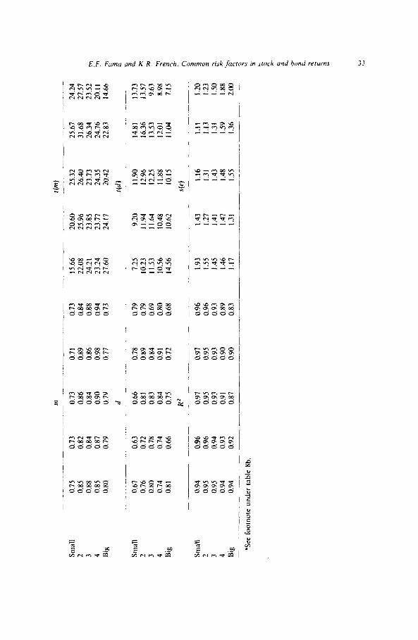
Sn1

all

0.75

0.

73

2 0.

85

0.82

3

0.88

0.

84

4 0.

85

0.87

Ij

ig

0.x0

0.

79

Smal

l 0.

67

0.63

2

0.76

0.

72

3 0.

80

0.78

4

0.74

0.

74

nig

0.81

0.

66

Smal

l 0.

94

0.96

2

0.95

0.

96

3 0.

95

0.94

4

0.94

0.

93

Big

0.94

0.

92

_-

._

"See

kmn

ote

unde

r ta

ble 8b

.

0.73

0.

86

0.84

0.

90

0.79

cl

0.71

0.

73

15.6

6 0.

89

0.84

22

.08

0.86

0.

88

24.2

1 0.

98

0.94

23

.24

0.77

0.

73

27.M

)

0.66

0.

81

0.83

0.

84

0.75

HZ

0.97

0.

95

0.93

0.

91

0.87

0.78

0.

79

7.25

0.

19

0.79

10

.23

0.84

0.

69

II.5

3 0.

91

0.80

10

.56

0.72

0.

68

14.5

6

____

_

0.97

0.

96

1.93

0.

95

0.96

1.

55

0.93

0.

93

1.45

0.

90

0.89

1.

46

0.90

0.

83

1.17

_~

___

--

20.6

0 25

.96

23.8

5 23

.77

24.1

7

9.20

11

.94

Il.6

4 10

.48

10.6

2 --

1.43

1.

27

1.41

1.

47

1.31

-_

_

dm)

~-_

-_

I 25

.32

25.6

7 24

.24

26.4

0 31

.68

27.5

7 23

.73

26.3

4 23

.52

24.3

5 24

.76

20.1

1 20

.42

22.8

3 14

.66

f@) 11

.90

12.9

6 12

.25

11.8

8 IO

.15

s(e)

I.16

I.31

1.

43

1.48

1.

55

14.8

1 13

.73

16.3

6 13

.57

13.5

3 9.

63

12.0

1 X.

98

II.0

4 7.

15

___-

-

1.11

1.

20

1.13

1.

23

1.31

1.

50

1.59

1.

88

1.36

2.

00

Table 8b

Regresstons ofswess returns on government and corporate bonds (in percent1 on the stock-market

returns. R.UO. S.UB. and H.tfL. and the bond-market returns. TERJI and DEf: July 1963 to

December 1991. 3-t: months.’

I-SG 66IOG .Aaa .-\a .A Baa LG

h - 0.03 - 0.04 - 0.02 0.00 0.00 0.0’ 0.18 ribI - 1.34 - 3.14 - 2.96 0.06 I .05 I .99 7.39

5 - 0.00 - 0.03 - 0.03 - 0.01 0.00 0.06 0.16 r(s) - 0.68 - 2.30 - 3.17 - 2.55 0.80 1.09 5.09

/I 0.02 - 0.00 - 0.01 - 0.00 0.00 0.03 0.00 f(lll 1.76 - 0.00 - 1.36 - 0.17 0.52 1.72 0.12

V, 0.45 0.71 1.02 0.99 1.00 1.01 0.79 t(trll 32.09 39.55 102.65 130.93 139.1 I 57.34 19.56

Cl 0.15 0.29 0.95 0.97 I .02 1.07 0.94 t(ll) 9.16 8.25 50.04 67.05 74.00 31.77 I’.09

R2 0.130 0.87 0.97 0.9s 0.98 0.9 I 0.58 S(Z) 0.56 0.73 0.40 0.30 0.29 0.70 1.63

_ _

‘R.\IO, the orthogonalized market return. is the sum of intercept and residuals from the represston of R.WRF on .S.\fB. H.LIL. TER.W, and DEF. R.ll 1s the value-ueighted monthly percent return on all stocks in the 25 size-BE .tfE portfolios. plus the negative-BE stocks excluded from the portfoltos. RF is ths one-month Treasury btll rate, observed at the beginning of the month. S.LfB (smdll mtnus big). the return on the mimicking portfolio for the common size factor tn stock returns, is the dtfference each month between the simple aberage of the returns on the three small-stock portioitos (S L. 5’ .\I. and S Hl and the simple aterage of the returns on the three big-stock portfoltos

(5 L. B .If. and B Hi fl.\/L (htgh minus low). the return on the mimicking portfolio for the common book-to-market equtty factor m returns, is the dtfference each month between the simple alerage of the returns on the t&o hi!h-BE .A/& portfolios 1.5 H and B i-l) and the average of the returns on the two low-BE .ME portfoltos (S f. and B L). TER.Lf is LTG-RF, where LX is the long-term government bond return. DEF IS CB-LTG, where CB is the return on a proxy for the market portfolto of corporate bonds.

The seben bond portfolios used as dependent variables m the excess-return regressions are I- to j-year and 6- to IO-year governments (1-S and &lOG) and bonds rated .Aaa. Aa. A. Baa, and

belou Baa (LG, by Moody’s The 25 size-BE.‘.LfE stock portfolios are formed as follows. Each year I from 1963 to 1991 XYSE quinttle breakpoints for size (LIE. stock price times shares outstandinp).

measured at the end of June. are used to allocate SYSE. Amer. and NASD.A.Q stocks to fire size qutnttles. NYSE quinttie breakpoints for BE .CfE are also used to allocate NYSE. .Amex. and S;\SD.AQ stocks to tire-book-to-market equity quintiles. In BE .L/E. BE is book common equity for the fiscal year endtng tn calendar year I - I. and .\fE ts for the end of December oft - 1. The 25 stze-BE .5/E portfolios are the intersections of the fi\e size and the five BE .ME groups. Vnlue- welshted monthly percent returns on the portfolios are calculated from July of year r to June of I - I.

R2 and the resdtual standard error. hIti), are adJusted for degrees of freedom.

Bond portfolio

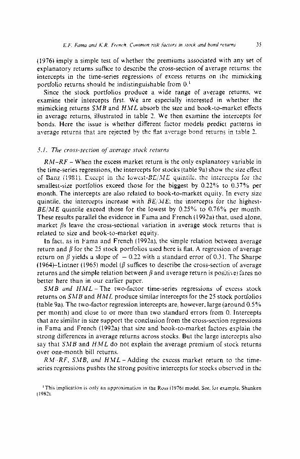
E. F. Fmnu und R. R. French. Common rd fucrors in srock und bond renm~s 35

(1976) imply a simple test of whether the premiums associated with any set of explanatory returns suffice to describe the cross-section of average returns: the intercepts in the time-series regressions of excess returns on the mimicking portfolio returns should be indistinguishable from 0.’

Since the stock portfolios produce a wide range of average returns, we examine their intercepts first. We are especially interested in whether the mimicking returns S,CIB and HML. absorb the size and book-to-market effects in average returns, illustrated in table 2. We then examine the intercepts for bonds. Here the issue is whether different factor models predict patterns in average returns that are rejected by the flat average bond returns in table 2.

3.1. The cross-section oj’acerage stock returns

R&f-RF - When the excess market return is the only explanatory variable in the time-series regressions, the intercepts for stocks (table 9a) show the size effect of Banz (1981). Except in the lowest-BE/ME quintile. the intercepts for the smallest-size portfolios exceed those for the biggest by 0.22% to 0.37% per month. The intercepts are also related to book-to-market equity. In every size quintile, the intercepts increase with BE/ME; the intercepts for the highest- BE/ME quintile exceed those for the lowest by 0.25% to 0.76% per month. These results parallel the evidence in Fama and French (1992a) that, used alone, market fls leave the cross-sectional variation in average stock returns that is related to size and book-to-market equity.

In fact, as in Fama and French (1992a), the simple relation between average return and /3 for the 25 stock portfolios used here is flat. A regression of average return on /J yields a slo’pe of - 0.22 with a standard error of 0.31. The Sharpe (1964)-Lintner (1965) model (/I suffices to describe the cross-section of average returns and the simple relation between /? and average return is positive) fares no better here than in our earlier paper.

SMB and HML - The two-factor time-series regressions of excess stock returns on SMB and HML produce similar intercepts for the 25 stock portfolios (table 9a). The two-factor regression intercepts are, however, large (around 0.5% per month) and close to or more than two standard errors from 0. Intercepts that are similar in size support the conclusion from the cross-section regressions in Fama and French (1992a) that size and book-to-market factors explain the strong differences in average returns across stocks. But the large intercepts also say that S.LfB and HML. do not explain the average premium of stock returns over one-month bill returns.

RM-RF, S.CfB, and H,LIL -Adding the excess market return to the time- series regressions pushes the strong positive intercepts for stocks observed in the

‘This implication is only an approximation in the Ross (19761 model. Ser. for example. Shanken (1982).

Tab

le

Ya

lntr

rce

prs

fr

om

e

xce

ss s

tuc

k

retu

rn

reg

ress

ion

s fo

r 25

st

uc

k

pu

rtfu

lios

form

ed

o

n

size

a

nd

b

oo

k-t

o-m

ark

et

eq

uity

: Ju

ly

1963

IO

D

ec

em

be

r IY

YI,

342

mo

nth

s.”

Bo

ok

-to

-ma

rke

t e

qu

ity

(HE/

ME)

q

uin

tile

s

Size

qu

inlil

e

Small

2 3 4 U

ig

Low

2

0.31

0.

62

0.35

0.

63

0.34

0.

58

0.4

1 0.

27

0.34

0.

30

t, I(

4

3 4

Hig

h

Low

2

3 4

Hig

h

~~

(i)

K(r

) -

W’(r

) =

(I +

OI~

‘ER

M(I

) +

dD

EF

(f)

+ t

$r)

0.71

0.

80

0.92

0.

75

1.73

2.20

2.

61

2.87

0.

77

0.75

0.

93

0.93

I.9

1 2.

60

2.85

3.

03

0.60

0.

73

0.89

I.0

0 I .

9Y

2.28

3.

01

3.1

I 0.

4’)

0.69

0.

96

1.34

1.01

1.96

2.X8

3.

35

0.25

0.

50

0.53

1.3

5 1.2

7 1.1

7 2.

36

2.14

(ii)

R(r

) -

RF

(r)

= u

+ ~

[RM

(I)

- R

F(r

)]

+ (

$0

sm;III

-

0.22

0.

15

0.30

0.

42

0.54

-

O.YO

0.

73

1.54

2.19

2.

53

2 -

0. I

X 0.

17

0.36

0.

3’)

0.53

-

1.00

I .05

2.

35

2.7Y

3.

01

3 -

0. I

6 0.

1s

0.23

0.

39

0.50

-

1.12

1.25

1.n2

3.20

3.

19

4 -

0.05

-

0.14

0.

12

0.35

0.

57

- 0.

50

- 1.5

0 1.2

0 2.

91

3.71

Big

-

0.04

-

0.07

-

0.07

0.

20

0.21

-

0.4Y

-

0.95

-

0.70

1.8

9 1.4

1

SIl

l;Lll

0.24

2

0.52

3

0.52

4

0.69

B

ig

0.76

Smnl

l -

0.34

2

-0.1

1 3

- 0.

1 I

4 0.

09

Big

0.

21

(iii)

X(r)

-

RF

(I)

= u

+ s

SMtq

r)

+ h

lfM

L&

) +

t(r

)

0.46

0.

49

0.53

0.

55

0.97

I.9

2 2.

24

0.58

0.

64

0.58

0.

64

2.00

2.

40

2.76

0.

61

0.52

0.

60

0.66

2.

00

2.58

2.

25

0.39

0.

50

0.62

0.

79

2.78

1.

55

2.07

0.

52

0.43

0.

51

0.44

3.

41

2.23

1.

84

(iv)

K(r

) -

W(r

) =

0 +

h[R

M(r

) -

RF(

r)]

+ sS

M&

I) +

h/IM

L(f)

+ V(

I)

- 0.

12

- 0.

05

0.01

0.

00

- 3.

16

- 1.

47

- 0.

73

- 0.

01

0.08

0.

03

0.02

-

1.24

-

0.20

1.

04

0.04

-

0.04

0.

05

0.05

-

1.42

0.

47

- 0.

47

- 0.

22

- 0.

08

0.03

0.

13

I .07

- 2.

65

- 0.

99

- 0.

05

-0.1

3 -

0.05

-

0.16

3.

27

- 0.

67

- 1.

46

Sm;il

l -

0.35

2

- 0.

1 I

3 -

0.12

4

0.0X

B

ig

0.21

~~

_.__

_

‘See

fo

otno

te

unde

r ta

ble

9c.

(v)

H(l)

-

RF

(f)

= u

+ h

[RM

(r)

- R

F(r

)]

+ s

SMB

(r)

+ h

HM

L(r

) +

ntT

ER

M(r

) +

dD

EF

(r)

+ &

)

- 0.

I3

- 0.

05

0.0

I 0.

00

- 3.

24

- 1.

58

- 0.

79

- 0.

02

0.0x

0.

04

0.02

~

1.29

-

0.24

1.

10

0.04

-

0.03

0.

06

0.05

-

1.45

0.

48

- 0.

42

- 0.

22

- 0.

08

0.04

0.

I 3

1.04

-

2.67

-

0.94

-

0.05

-

0.13

-

0.06

-

0.17

3.

29

- 0.

72

- 1.

46

_ ~~

~ ~

~~

~__

.~~

~.~

.

2.52

2.

49

2.61

2.

56

2.66

2.

61

2.51

2.

85

2.20

1.

70

0.22

0.

14

0.51

0.

34

0.7

I 0.

56

0.33

I .

24

0.69

-

I.41

0.20

0.

09

0.67

0.

29

0.79

0.

56

0.47

1.

23

0.73

-

I.51

Table Yb

portfolios. Jul> 1963 to December 1931. 343 months.’

Bond portfolIo

1-K 6-IOG ‘AU .A.l A B&I LG

II) R(r) - Rf(tl = tt 4 mTER.LIItI + <IfIEf-ltl + ettt

0.08 0.09 - 0.02 - 0.00 - 0.00 0.06 0.06

2.70 7.16 - 1.10 - 0.55 - 0.2Y I .42 0.67

Ilil Rlr) - RF(t) = (I 4 h[R.\!~tl - RF(t)] + fir1

0.08 0.08 - 0.03 - 002 - 0.0 I 0.0-l 0.M) I.27 0.76 - 0.21 - 0.15 - 0.1 I 0.37 0.03

luil R(rl - RF(t) = LI + sS.tlB(t) + hH.LfLlt) + e(t)

0. I1 0. I6 0.07 0.07 0.0’ 0.1 I 0.08

1.70 I .47 0.52 0.58 0.55 0.82 0.58

(1~) R(r) - RF(t) = LI + h[RM(t) - RF‘ltl] + s.S.\IBltl + ItH.VLltl + CICI

0.06 0.07 - 0.07 - 0.07 - 0.08 - 0.05 - 0.1 I

0.8Y 0.62 - 0.62 - 0.64 - 0.69 - 0.41 - 1.00

(\I R~ri - RF(t) = (1 + h[R.\l(t) - RFltl] t sS.\/51t1 + hff.\IL(t~

+ ntTER.Lf(t) + riDEflt) + p(t)

0.09 0.1 I - o.Oil - 0.00 - 0.00 0.02 - 0.07

2.8-l 1.77 - 0.17 - 0.25 - 0.57 0.52 _ 0.77

‘See footnote under table Yc.

tuo-factor (.S.LfB and H.CIL) regressions to values close to 0. Only thr22 of the 25 intercepts in the three-factor regressions differ from 0 by more than O.Z’?,b per month: 16 are wtthtn 0.144 o f 0. Intercepts close to 0 say that the regressions that use R.11-RF. S.lIB. and HAIL to absorb common time-series variation in returns do a good job explaining the cross-section of average stock returns.

There is an interesting story for the smaller intercepts obtained when the excess market return is added to the two-factor (S.CfB and H,CIL) regressions. In the three-factor regressions. the stock portfolios produce slopes on R.&RF clos2 to I. The average market risk premium (0.33% per month) thzn absorbs the similar strong positive intercepts observed in the regressions of stock returns on .S.\fB and H.LJL. In short, the size and book-to-markzt factors can sxplain the differences in averagz returns across stocks. but the markzt factor is needed to explain why stock returns are on average above the one-month bill rate.

TER.lf cud DEF - Table 9a shows that adding the term-structure factors, TER.11 and DEF. to the tim2-series regressions for stocks has almost no effect on the intercepts produced by the three stock-market factors. Likewise. in spite of the strong slopes on TER.tf and DEF when they are used alone to explain stock

E.F. Funu md R. R. Frmch. Conrnwn rd lircrors in .uuck und bond rr~urrrs 39

Table 9c

F-startstics testing the intercepts in the excess-return regressions against 0 and matching probability levels of bootstrap and F-dtstrtbutions.”

Regression (from tables 9a and 9b)

(i) (ii) (iii) (iv) (v)

F-statistic Probability level

2.09 !.91 1.75 1.56 1.66

Bootstrap F-distribution

0.998 0.996 0.985 0.95 1 0.971 0.999 0.996 0.990 0.96 I 0.975

--__

“R.11 is the value-weighted monthly percent return on all stocks in the 25 size-BE .lfE portfolios. plus the negative-BE stocks excluded from the 25 portfolios. RF 15 the one-month Treasury bill rate. observed at the beginning of the month. S.LfB (small minus big), the return on the mimicking portfolio for the common size factor in stock returns. is the difference each month between the simple average of the returns on the three small-stock portfolios (5 L, S’XI. and S H) and the simple average of the returns on the three big-stock portfolios IB L. B’.LI, and B H). H,ML (high minus low). the return on the mimicking portfolio for the common book-to-market equity factor in returns. is the difference each month between the simple average of the returns on the two high-BE .WE portfolios (S,‘H and B H) and the average of the returns on the two low-BE .bfE portfolios (S L and B LI. TER.W is LX-RF. where LX is the long-term government bond return. DEF is CB-LK. where CB is the return on a proxy for the market portfoho of corporate bonds.

The seven bond portfolios used as dependent variables in the excess-return regressions are I- to j-year And 6- to IO-year governments (I-5G and CLOG) and corporate bonds rated Aaa, Aa. A, Baa. and below Baa (LG) by Moody’s, The 25 size-BE .%I E stock portfolios are formed as follows. Each year f from 1963 to I991 NYSE quintile breakpoints for stze (.WE. stock price times shares outstanding). measured at the end of June, are used to allocate NYSE. Amex. and N.ISDAQ stocks to live size quintiles. NYSE quintile breakpoints for BE .tfE are also used to allocate NYSE. Amex, and N.ASDAQ stocks to five book-to-market equity quintiles. In BE .LfE. BE is book common equity for the tiscal year ending in calendar year I - I. and :1fE is for the end of December oft - I. The 25 size-BE .tfE portfolios are the intersections of the five size and the five BE .LfE groups. Value-vveightsd monthly percent returns on the portfoltos are calculated from July of year c to June oft+ I.

Regressions (I~+v) in table 9c correspond to the regressions tn tables 9a and 9b. The F-stattstic is

F = (.-l’_r-‘?t)(.v - K - f + I),(L*(.V - K)*W,,,).

where .V = 342 observations. L = 31 regressions, K is 1 plus the number ofexplanatory variables in the regression. A is the (column) vector of the 32 regression intercepts. Z (L x L) is the unbiased covariance matrix of the residuals from the 32 regressions. and o,.r is the diagonal element of (.Y’X)-r corresponding to the intercept. Gibbons, Ross. and Shanken (19891 show that this statistic has an F-distribution with L and N - K - f. i I degrees of freedom under the assumption that the returns and explanatory variables are normal and the true intercepts are 0.

In the bootstrap simulations, the slopes (with intercepts set to 0). explanatory variables. and residuals from the regressions for July 1963 to December 1991 in tables 3 to 7 are used to generate 342 monthly excess returns for the 25 stock and seven bond portfolios for each regression model. These model returns and the exrlanatory returns. R.Lf-RF. S.LfB. H.CfL, TER.Lf. and DEF, for July 1963 to December 1991, are the population for the stmulations. Each simulation takes a random sample. with replncement. of 342 paired observations (the same set of observations for each of the five regression models) on the model returns and the explanatory variables. and estimates the regressicns. For each model. the table shows the proportion of 10.000 simulations rn which the F-Xdttstic is smaller than the empirical estimate. The table also shows the probability that a value drawn from an F-distribution is smaller than the empirical estimate.

returns (table 3). the two variables produce intercepts close to the average excess returns for the 25 stock portfolios in table 2.

The reason for these results is straightforward. The average TER.Ll and DEF returns (the average risk premiums for the term-structure factors) are puny, 0.06% and 0.02% per month. The high volatility of TER.Ll and DEF (table 2) allows them to capture substantial common variation in bond and stock returns in the two-factor regressions of table 3 and the five-factor regressions of table 8. But the low average TER,LI and DEF returns imply that the two term-structure factors can’t explain much of the cross-sectional variation in average stock returns.

5.2. The cross-section of average hod retwrrs

Tables 3. 7b and 8b say that the common variation in bond returns is dominated by the bond-market factors, TERM and DEF. Oniy the low-grade bond portfolio (LG) has nontrivial slopes on the stock-market factors when TERM and DEF are in the bond regressions. Like the average values of TERM and DEF. the average excess returns on the bond portfolios are close to 0 (table 2), so it is not surprising that the intercepts in the time-series regressions for bonds (table 9b) are close to 0.

Do low average TERM and DEF premiums imply that the term-structure factors are irrelevant in a well-specified asset-pricing model? Hardly. TER.Ll and DEF are the dominant variables in the common variation in bond returns. Moreover, Fama and-French (1989) and Chen (1991) find that the expected values of variables like TER;LI and DEF vary through time and are related to business conditions. The expected value of TER.CJ, the term premium for discount-rate risks, is positive around business cycle troughs and negative near peaks. The expected value of the default premium in DEF is high when economic conditions are weak and default risks are high, and it is low when business conditions are strong. Thus, the common sensitivity of stocks and bonds to TERM and DEF implies interesting intertemporal variation in expected stock and bond returns.

j.3. Joiut tests on the regression intercepts

We use the F-statistic of Gibbons, Ross. and Shanken (1989) to formally test the hypothesis that a set of explanatory variables produces regression intercepts for the 32 bond and stock portfolios that are all equal to 0. The F-statistics, and bootstrap probability levels, for the five sets of intercepts produced by the explanatory variables in tables 3 to 8 are in table 9c.

The F-tests support the analysis of the intercepts above. The tests reject the hypothesis that the term-structure returns, TER,Ll and DEF. suffice to explain the average returns on bonds and stocks at the 0.99 level. This confirms the

conclusion, obvious from the regression intercepts in table 9a, that the low average TERM and DEF returns cannot explain the cross-section of average stock returns. The F-test rejects the hypothesis that RAWRF suffices to explain average returns at the 0.99 level. This confirms that the excess market return cannot explain the size and book-to-market effects in average stock returns. The large positive intercepts for stocks observed when SicIB and HAlL are the only explanatory variables produce an F-statistic that rejects the zero-intercepts hypothesis at the 0.98 level.

In terms of the F-test. the three stock-market factors, R&I-RF, SMB, and HML, produce the best-behaved intercepts. Nevertheless, the joint test that all intercepts for the seven bond and 25 stock portfolios are 0 rejects at about the 0.95 level. The rejection comes largely from the lowest-BE’JIE quintile of stocks. Among stocks with the lowest ratios of book-to-market equity (growth stocks), the smallest stocks have returns that are too low ( - 0.34% per month, t = - 3.16) relative to the predictions of the three-factor model, and the biggest stocks have returns that are too high (0.21% per month, t = 3.27). Put a bit differently, the rejection of a three-factor model in table 9c is due to the absence of a size effect in the lowest-BE,‘ME quintile. The five portfolios in the lowest- BE/ME quintile produce slopes on the size factor SMB that are strongly negatively related to size (table 6). But unlike the other BE/ME quintiles, average returns in the lowest-BE/ME quintile show no relation to size (table 2).

Despite its marginal rejection in the F-tests, our view is that the three-factor model does a good job on the cross-section of average stock returns. The rejection of the model simply says that because R,WRF, S,LIB, and HML absorb most of the variation in the returns on the 25 stock portfolios (the typical R’ values in table 6 are above 0.93). even small abnormal average returns suffice to show that the three-factor model is just a model, that is, it is false. To answer the important question of whether the model can be useful in applications, the interesting result is that only one of the 25 three-factor regression intercepts for stocks (for the portfolio in both the smallest-size and the lowest-BE/ME quintiles) is much different from 0 in practical terms.

Indeed, our view is that the three-factor regressions that use RM-RF, SMB, and H,bfL to explain average returns do surprisingly well, given the simple way the mimicking returns SMB and HML for the size and book-to-market factors are constructed. The regressions produce intercepts for stocks that are close to 0, even though SMB and HML surely contain some firm-specific noise as proxies for the risk factors in returns related to size and book-to-market equity.

Adding the term-structure returns. TER.Cf and DEF, to regressions that also use R.11-RF, S.bfE, and H.ClL as explanatory variables increases F. The larger F comes from bonds. The five-factor regression intercepts and R’ values for stocks are close to those produced by the three stock-market factors. But for bonds, adding TER.Cf and DEF results in much lower residual standard errors. and the increased precision pushes the five-factor intercepts for the two

government bond portfolios beyond two standard errors from 0. The two intercepts are. however, rather small, 0.09O 0 and 0. I 1% per month.

The three stock-market factors produce a lower F, but we think the five-factor regressions provide the best model for returns and average returns on bonds and stocks. TER.Lf and DEF dominate the variation in bond returns. And the variation in the expected values of TERJf and DEF with business conditions is an interesting part of the variation through time in the expected returns on stocks and bonds that is missed by the F-test, which is concerned only with long-term average returns.

6. Diagnostics

In this section we check the robustness of our inference that five common risk factors explain the cross-section of expected stock and bond returns. We first use the residuals from the five-factor time-series regressions to check that the regressions capture the variation through time in the cross-section of expected returns. We then examine whether our live risk factors capture the January seasonals in stock and bond returns. Next come split-sample regressions that use one set of stocks in the explanatory returns and another. disjoint, set in the dependent returns. These tests address the concern that the evidence of size and book-to-market factors in the regressions above is spurious, arising only because vve use size and book-to-market portfolios for both our dependent and explanatory returns. The last and most interesting tests examine whether the stock-market factors that capture the average returns on size-BE,‘.LfE portfolios work as well on portfolios formed on other variables known to be informative about av’erage returns. in particular, earnings, price and dividend,‘price ratios.

There is evidence that stock and bond returns can be predicted using (a) dividend yields (D,,P), (b) spreads of low-grade over high-grade bond yields (default spreads, DFS), (c) spreads of long-term over short-term bond yields (term spreads. TS), and (d) short-term interest rates. [See Fama (1991) and the references therein.] If our five risk factors capture the cross-section of expected returns. the predictability of stock and bond returns should be embodied in the explanatory returns (the month-by-month risk premiums) in the five-factor regressions. The regression residuals should be unpredictable. To test this hypothesis. we estimate the 32 time-series regressions,

e,(t + 1) = k,, + k,D(r) P(r) -I- k2DFS(r) + k,TS(t) + k,RF(r)

+ r/Jr + 1). (2)

The r,(t + I)in (2) are the time series of residuals for our 25 stock and seven bond portfolios from the five-factor regressions of table 7. The dividend yield, D(t). P(t), is dividends on the value-weighted portfolio of NYSE stocks for the year ending in month t divided by the value of the portfolio at the end oft. The default spread, DFS(t), is the difference at the end of month r between the yield on a market portfolio of corporate bonds and the long-term government bond yield (from Ibbotson Associates). The term spread. TS(r), is the difference between the long-term government bond yield at the end of month c and the one-month bill rate, RF(r).

The estimates of (2) produce no evidence that the residuals from the five-factor time-series regressions are predictable. In the 31 regressions, 15 produce negative values of R’ (adjusted for degrees of freedom). Only four of the 32 R’ values exceed 0.01; the largest is 0.03. Out of 1X (32 x 4) slopes in the residual regressions. ten are more than two standard errors from 0; they are split evenly between positive and negative values. and they are scattered randomly across the 32 regressions and the four explanatory variables.

The fact that variables known to predict stock and bond returns do not predict the residuals from our live-factor regressions supports our inference that the five risk factors capture the cross-section ofexpected stock and bond returns. The residual tests are also interesting information on a key regression specifica- tion. Since we estimate regression slopes on returns for the entire 1963-1991 period, we implicitly assume that the sensitivities of the dependent returns to the risk factors are constant. If the true slopes vary through time, the regression residuals may be spuriously predictable. The absence of predictability suggests that the assumption of constant slopes is reasonable, at least for the portfolios used here.

Since the work Roll (1983) and Keim (1983). documenting that stock returns, especially returns on small stocks, tend to be higher in January, it is standard in tests of asset-pricing models to look for unexplained January effects. We are leery of judging models on their ability to explain January seasonals. If the seasonals are, in whole or in part, sampling error, the tests can contain a data- snooping bias toward rejection [Lo and MacKinlay (1990)]. Nevertheless, we test for January seasonals in the residuals from our five-factor regressions. Despite our fears. we find that, except for the smallest stocks. residual January seasonals are weak at best. The strong January seasonals in the returns on stocks and bonds are largely absorbed by strong seasonals in our risk factors.

Table 10 shows regressions of returns on a dummy variable that is 1 in January and 0 in other months. The regression intercepts are average returns for non-January months, and the slopes on the dummy measure differences between average January returns and average returns in other months.

Tabl

e 10

Test

s fo

r Ja

nuar

y se

ason

als

in

the

depe

nden

t re

turn

s,

expl

anat

ory

retu

rns,

an

d re

sidu

als

from

th

e fiv

e-fa

ctor

re

gres

sion

s:

July

19

63

IO D

ecem

ber

1991

, 34

2 m

onth

s.’

ICac

lor

u

HM-RF

KM0

SMB

t/ML

TERM

DEF

0.31

0.

40

0.05

0.

2 I

0.10

_

- 0.

07

Stoc

k po

rtfo

lio

t~t~

/Ar t:

Low

-

0. I3

M

r/A

re ?

0.

24

NT/MI: 3

0.31

U

E/M

E

4 0.

37

BE/

ME

Hig

h 0.

40

BE/

ME

Low

BE

/ME

2

HE/M

E 3

BE/M

I:

4

HE/M

E H

igh

0.20

0.

37

0.53

0.

4x

0.55

BE/M

E Lo

w

0.24

B

E/M

E 2

0.42

HE

/At

E 3

0.43

tlE/ME4

0.52

nEjnlE H

igh

0.60

K(r

) =

u +

bJAN

(r)

+ r

u b

w

l(b)

Five

-fact

or

expt

anal

ory

retu

rns

R2

I .49

I .

22

I .67

0.

00

1.19

2.

03

I .70

0.

00

2.74

0.

30

4.96

0.

06

2.29

I .

53

4.70

0.

06

0.41

0.

56

- 0.

69

- 0.

00

I.10

- 0.

8 I

3.56

0.

03

Exce

ss

stoc

k re

turn

s

6.31

5.

62

5.91

6.

29

7.39

2.92

4.

17

3.95

4.

32

5.76

2.35

2.

87

3.06

3.

51

4.53

Smat

trst

-siz

e qu

intit

c -

0.30

4.

23

0.05

0.

03

4.27

0.

05

0.90

4.

93

0.06

1.

14

5.55

0.

08

1.20

6.

3 I

0.10

Size

qu

intit

e 2

0.48

2.

04

0.00

I.0

4 3.

34

0.03

I .

63

3.48

0.

03

I .65

4.22

0.

05

1.66

4.

99

0.07

Size

qu

inlit

e 3

0.62

I .

78

0.00

1.

31

2.57

0.

02

t .47

2.99

0.

02

I.92

3.6X

0.

04

t.9t

4.12

0.

04

- 0.

12

I.51

- 1.

17

4.09

0.

04

- 0.

05

0.56

-

0.57

2.

01

0.00

-

0.06

0.

69

- 0.

81

3.06

0.

02

- 0.

06

0.76

-

1.02

3.

57

0.03

-

0.09

1.

13

- I.4

1 4.

94

0.06

0.02

-

0.23

0.

21

- 0.

74

- 0.

00

0.00

-

0.04

0.

04

- 0.

15

- 0.

00

0.04

-

0.55

0.

62

- 2.

16

0.01

0.

02

- 0.

22

0.2x

-

0.97

~

0.00

-

0.01

0.

12

- 0.

14

0.49

-

0.00

0.04

-

0.49

0.

50

~ 1.

74

0.00

0.03

-

0.41

0.

42

- 1.

48

0.00

0.

07

- 0.

x0

0.x3

-

2.90

0.

02

0.04

-

0.46

0.

52

- 1.

80

0.00

0.

03

- 0.

34

0.33

-

1.15

0.

00

h I(

4 ((

4 R2

Five

-fact

or

regr

essi

on

resi

dual

s

BE

/ME

L

ow

B

EfM

E

2 LX

/ME

3

BE

/ME

4

nE/M

E

Hig

h

LIE

/ME

L

ow

N

Ejh

fE

2 B

E/M

E

3 S

E/M

E

4 B

E/M

E

Hig

h

Bo

nd

p

ort

folio

I S

C

- 0.

00

6-I

o<;

-- O

.(K

) A

a;l

0.0

I A

;1

0.00

A

0.

0 I

Baa

O

.lNJ

LG

-

0.00

_

‘JA

N(r

) is

a d

um

my

vari

able

th

at

is I

if

mo

nth

I

is J

anu

ary

and

0

oth

erw

ise.

R

MO

is

th

e su

m

of

the

inte

rcep

t an

d

resi

du

als

fro

m

the

reg

ress

ion

o

f

- 0.

04

0.12

-

0.40

-

0.1

I 0.

23

- 0.

79

- 0.

17

0.62

-

2.17

-

0.1

I 0.

53

- I.8

5 0.

12

- 0.

60

2.0x

0.

14

- 0.

29

I.01

0.19

-

0.17

0.

58

0.39

0.

21

0.40

0.

52

0.68

0.37

0.

27

0.23

0.

37

0.32

Siz

e q

uin

tile

4

1.12

1.

16

0.95

-

0.00

1.

77

0.68

1.

65

0.00

2.

0X

I .40

2.

1 I

0.0

I 3.

12

1.88

3.

24

0.03

4.

45

2.15

4.

00

0.04

Big

ges

t-si

ze

qu

inti

le

0.34

1.

34

0.35

-

0.00

1.

11

I .02

1.

19

0.00

1.

11

0.92

1.

28

0.00

2.

31

1.54

2.

85

0.02

3.

38

1.17

3.

59

0.03

Exc

ess

bo

nd

re

turn

s

0.04

-

0.46

0.

46

- 1.

60

0.06

-

0.73

0.

73

- 2.

54

0.08

-

0.93

0.

93

- 3.

27

0.03

-

0.37

0.

34

- I.1

7 0.

00

- 0.

03

0.03

-

0.09

0.38

-

0.48

I .

67

- 0.

00

0.00

-

0.02

-

0.17

0.

16

- 0.

57

0.08

-

0.09

0.

31

0.25

-

0.18

0.

63

Fiv

e-fa

cto

r re

gre

ssio

n

resi

du

als __

~~

0.00

0.02

0.

03

0.00

-

0.00

0.00

-

0.00

-

0.00

-

0.00

-

0.00

RI%

-RI’

w

Shf

n,

//bfl

.. T

l:‘R

hf,

and

D

EP

. K

M

is t

he

valu

e-w

eig

hte

d

mo

nth

ly

sto

ck-m

arke

t re

turn

. R

F

is t

he

on

e-m

on

th

Tre

asu

ry

bil

l ra

te,

ob

serv

ed

at

the

beg

inn

ing

o

l’th

e m

on

th.

SM

U

and

f/M

L ar

e th

e re

turn

s o

n t

he

mim

icki

ng

p

ort

folio

s fo

r th

e si

ze a

nd

b

oo

k-to

-mar

ket

equ

ity

fact

ors

in

sto

ck

retu

rns.

7’

k’R

M

is L

TG

-RF

, w

her

e LT

G

is t

he

lon

g-t

erm

g

ove

rnm

ent

bo

nd

re

turn

. D

EF

is

Cn-

LTG

, w

her

e C

B i

s th

e re

turn

o

n a

pro

xy

for

the

mar

ket

po

rtro

lio

of

corp

ora

te

bo

nd

s.

Th

e se

ven

bo

nd

p

ort

folio

s ar

e I-

to

5-y

ear

and

6-

to

IO-y

ear

go

vern

men

ts

(I-5

G

and

GIO

G)

and

b

on

ds

rate

d

Aaa

, A

a,

A.

Baa

, an

d b

elo

w

Baa

(L

G)

by

Mo

od

y’s,

T

he

25 s

ize-

-BE

/ME

p

ort

folio

s ar

e fo

rmed

as

th

e in

ters

ecti

on

s o

f in

dep

end

ent

sort

s o

f st

ock

s in

to

size

an

d

bo

ok-

to-m

arke

t eq

uit

y q

uin

liles

in

Ju

ne

of

each

ye

ar

fro

m

1963

-199

1.

Th

e va

riab

les

are

des

crib

ed

in m

ore

d

etai

l in

tab

le

8.

The table confirms that there are January season& in excess stock returns, and the seasonals are related to size. The slopes on the January dummy are all more than 1.91% per month and more than two standard errors from 0 for the portfolios in the two smallest size quintiles. Controlling for BE .ifE. the extra January return declines monotonically with increasing size. More interesting, the January seasonal in stock returns is also related to book-to-market equity. In every size quintile. the slopes on the January dummy tend to increase with BE ‘!Cf E. The extra January return for the two highest-BE .\JE portfolios in a size quintile is always at least 2.38% per month and 2.85 standard errors from 0.

January season& are not limited to stock returns. The slopes on the January dummy for corporate bonds increase monotonically from the Aaa to the LG portfolio. The extra January returns are 0.86’5b. 1.13%. and 1.56% per month for the A, Baa, and LG portfolios, and these extra average returns are at least 1.94 standard errors from 0.

If our five-factor time-series regressions are to explain the January seasonals in stock and bond returns. there must be January seasonals in the risk factors. Table 10 shows that, except for TERJI. the risk factors have extra January returns in excess of I % per month and at least I .67 standard errors from 0. The season& in the size and book-to-market factors are especially strong. The average S,LIB and H,tfL returns in January are 2.73% and 2.29% per month greater than in other months, and the extra January returns are 3.96 and 4.70 standard errors from 0. Indeed, like the excess returns on the 25 stock portfolios and the five corporate bond portfolios that are the dependent variables in the five-factor regressions. the extra January returns on the risk factors are generally much larger and more reliably different from 0 than the average returns for non-January months.

Finally, table 10 shows that the January seasonals in our risk factors largely absorb the seasonals in stock and bond returns. fn the regressions of the five-factor residuals on the January dummy. only the stock portfolios in the smallest-size quintile produce systematically posttive slopes: even these slopes are only one-quarter to one-tenth the positive January seasonals in the raw excess returns on the portfolios. If anything. the five-factor residuals for the remaining size quintiles show negative January seasonals, but the slopes on the January dummy for these stock portfolios. and for the bond portfolios, are small and mostly within two standard errors of 0. In short, whether spurious or real, the January seasonals in the returns on stocks and corporate bonds seem to be largely explained by the correspondin, u seasonals in the risk factors of our five-factor model.

In the time-series regressions for stocks. the dependent returns and the tvvo explanatory returns S:LIB and H.LlL are portfolios formed on size and

E.F. Fuamu umf K. R. French. Common risk /&torr WI stock md bond returns 17

book-to-market equity. Many readers worry that the apparent explanatory power of SLVB and N.CIf. is spurious, induced by the regression setup. We think this is unlikely. given that the dependent returns are based on much finer size and BE:.CfE sorts (25 portfolios) than the S.IIB and H.LIL returns. It also seems unlikely that we have stumbled on two mimicking returns for size and BE/ME factors that (a) measure strong common variation in the returns on 25 portfolios when really there is none, and (b) produce exactly the patterns in the regression slopes on S,bfB and HML needed to explain the size and book-to-market effects in the average returns on the 25 portfolios. Still, an independent test is of interest.

We split the stocks in each of the 25 size-BE ,LfE portfolios into two equal groups. One group is used to form the 25 dependent value-weighted portfolio returns for the time-series regressions. The other is used to form half-sample versions of the explanatory returns. RIM-RF. SMB. and HhfL. The roles of the two groups are then reversed. and another set of regressions is run. In this way we have two sets of regressions. In each set, the explanatory and dependent returns are from disjoint groups of stocks.

Without showing all the details, we can report that the results for the two sets of regressions of excess returns for 25 size-BEj’,LfE portfolios on disjoint versions of RM-RF. Slbff3, and H.bfL are similar to the full-sample results in tables 6 and 9. The slopes on RXf-RF, S&f& and H.CfL in the split-sample regressions are close to those in table 6, and the intercepts. like those for the full-sample three-factor regressions in table 9. are close to 0. In short, the split-sample regressions confirm that there are common risk factors in returns related to size and book-to-market equity. They also confirm that market, size, and book-to-market factors seem to capture the cross-section of average stock returns.

If anything, the split-sample regressions show less power to reject the hypothesis that R.Lf-RF, SMB, and H&IL capture the cross-section of average stock returns than the full-sample regressions. Since the 25 dependent portfolio returns in the split-sample regressions use half the available stocks. the portfolios are less diversified than those in table 6. Although the three-factor split-sample regressions produce high values of R’ (mostly greater than 0.88), they are a bit lower than those in table 6 (mostly greater than 0.9). As a result. the F-tests of the zero-intercepts hypothesis are weaker for the split-sample regressions than for the full-sample regressions.

6.4. Portfolios fbrtwd on E, P

The most interesting check on our inferences about the role of size and book-to-market risk factors in returns is to examine whether these variables explain the returns on portfolios formed on other variables known to be

informative about average returns. Table 11 shows summary statistics, as well as one-factor (RM-RF) and three-factor (R.LJ-RF. SMB, and HAIL) regressions for portfolios formed on earningsprice (E, P) and dividend/price (D.‘P) ratios.

The average returns on the E/P portfolios have the U-shape documented in Gaffe, Keim, and Westerfield (1989) and Fama and French (1992a). The portfolio of firms with negative earnings and the portfolio of firms in the highest-E/P quintile have the highest average returns. For the positive-E/P portfolios, average return increases from the lowest- to the highest-E/P quintile. This pattern is an interesting challenge for our risk factors.

Table I I

Summary statistics for value-weighted monthly excess returns (in percent) on portfolios formed on dividend price (D P 1 and earnings, price (E, P), and regressions of excess portfolio returns on (i) the excess market return (R.WRF) and (ii) the excess market return (R.Lf-RF) and the mimicking returns for the size ISCUB) and book-to-market equity (H.VL) factors: July 1963 to December 1991.

342 months.”

Ii) R(t) - RF(r) = a + b[RM(t) - RF(t)] + e(t)

(ii) R(r) - RF(t) = tz + b[Rhf(r) - RF(r)] + sS.CfB(r) + hH.VfQt) + e(t)

Purrfolio

Portfolios formed on E P Portfolios formed on D P _

Mean Std. r(mn) Mean Std. t(mn)

GO 0.72 7.77 1.72 0.48 7.36 1.20 Low 0.27 5.13 0.96 0.39 5.48 I .30 7

; 0.17 0.16 4.76 4.68 1.53 I .82 0.44 0.47 4.53 4.65 1.68 1.87 4 0.55 4.4s 2.27 0.57 4.33 1.42 Htgh 0.86 -I.%+ 3.30 0.56 3.86 2.67

Portfolios formed on E’P

Regression (i) Regression (ii)

Portfolio ‘1 h R? ll b 5 h R2

EPGO 0.13 1.37 (0.50) (‘4.70)

Low - 0.10 1.10 ( - 2.35, (57.42)

2 0.03 I.01 (0.46) (70.24)

3 0.04 0.99 (0.50) 161.62)

1 0.15 0.93 t 1.761 (49.78)

High 0.46 0.91 (3.69) (34.733

0.64 - 0.30 ( - 1.68)

0.9 I 0.04 (0.70)

0.91 0.03 (OAO,

0.91 - 0.00 ( - 0.11)

0.58 - 0.02 ( - 0.28)

0.78 0.08 11.01)

I.21 (27.82)

0.99 (66.75)

1.01 (61.17)

1 .oo (55.16)

0.98 (53.57)

I .03 (51.56)

I.13 (17.42)

- 0.01 ( - 0.55)

0.02 (1.01)

001 (0.40)

0.05 ( 1.95)

0.24 (8.34)

0.16 0.82 (6.10)

- 0.50 0.96 t - 19.73)

- 0.00 0.94 ( - 0.081

009 0.92 (3.86,

0.33 0.9 I ( lO.UI

0.67 0.91 (19.62)

Table I1 (continued)

Portfolios formed on D P

Regression (i) Regression (ii)

Portfolio U b R’ 0 b s h R’

D*P=O - 0.15 1.45 0.80 - 0.23 I.20 0.99 - 0.21 0.94 I - 0.86) (37.18) ( - 2.30) (49.45) (35.09) ( - 5.17)

Low - 0.1 I I.15 0.9 I 0.11 I .03 0.09 - 0.48 0.95 ( - 1.29) (59.15) (1.64) (65.09) (3.92) ( - 17.92)

2 - 0.01 1.04 0.96 0.06 1.01 - 0.01 - 0.14 0.96 ( - 0.19) (85.34) (1.17) (77.07) ( - 0.66) ( - 6.49)

3 0.04 0.99 0.93 - 0.03 I .02 0.02 0.14 0.94 (0.64) (69.14) ( - 0.44 (64.43) (0.72) (5.09)

4 0.17 0.9 I 0.9 1 0.04 0.98 - 0.06 0.30 0.91 (2.45) (58.42) (0.59) (66.51) ( - 2.80) (12.00)

High 0.24 0.72 0.73 - 0.01 0.85 - 0.05 0.54 0.8-t (2.22) (30.16) (0.16) (40.08) ( - 1.77) (15.04)

“Portfolios are formed in June of year r, 1963-1991. The dividend yield (D P) for year f is the dividends paid from July of I - 1 to June oft [measured using the procedure described in Fama and French (1988)]. divided by market equity in June of r - 1. The earnings price ratio (E/P) for year t is the equity income for the fiscal year ending in calendar year t - 1. divided by market equity in December of t - I. Equity income is income before extraordinary items. plus income-statement deferred taxes, minus preferred dividends. The quintile breakpoints for D.‘P or E’P are determined using only NYSE firms with positive dividends or earnings. Regression t-statistics are in parentheses. See table 7 for definitions of R,Lf-RF. S.Wf3. and H&IL.

Table It confirms the evidence in Basu (1983) that the one-factor Sharpe-Lintner model leaves the relation between average return and E,‘P largely unexplained. For the positive-E/P portfolios. the intercepts in the one- factor regressions increase monotonically, from - 0.20% per month (t = - 2.35) for the lowest-E/P quintile to 0.46% (t = 3.69) for the highest. The failure of the one-factor model has a simple explanation. The market j?s for the positive-E/P portfolios are all close to 1.0, so the one-factor model cannot explain the positive relation between E/P and average return.

In contrast, the three-factor model that uses RM-RF, SMB. and HML to explain returns leaves no residual E/P effect in average returns. The three-factor intercepts for the five positive-E P portfolios are within 0.1 of0 ( C’S from - 0.12 to 1.01). Interestingly, the three-factor regressions say that the increasing pattern in the average returns on the positive-E/P portfolios is due to their loadings on the book-to-market factor HML. The lowest positive-E P quintile has an HML slope, - 0.50, like those produced by portfolios in the lowest-BEIME quintile in the three-factor regressions in table 6. The highest-E/P quintile has an HML slope, 0.67, like those for portfolios in the highest-BE .UE quintile in table 6. Table 1 confirms that there is also a positive relation between E’P and BE/ME for our 25 portfolios formed on size and BE/ME.

Fama and French (1991bl find that lovv BE .tfE is characteristic of growth stocks. that is. stocks vvith persistently high earnings on book equity that result in high stock prices relative to book equity. High BE .\fE. on the other hand, is associated with distress. that is. persistently low earnings on book equity that result in low stock prices. The loadings on H.1fL in the three-factor regressions of table II then say that low-E P stocks have the low average returns typical of (low-BE.‘.CfE) growth stocks, while high-E P stocks have the high average returns associated with distress (high-BE’.!IE).

The negative-E. P portfolio produces the only hint of evidence against the three-factor model. In spite of the portfolio’s high average excess return (0.72% per month). the three-factor model says that its average return is O.?‘!/o per month too low, given its strong loadings on .S.!fB (1.13. like the smallest-size portfolios in table 6) and H.LfL (0.16. like the higher-BE .!fE portfolios in table 6). In other words, according to the three-factor model. the average return on this portfolio should be higher because its return behaves like those of small. relatively depressed. stocks. The three-factor intercept for the negative-E P portfolio is, however. only I.65 standard errors from 0.

In short. E/P portfolios produce a strong spread in average returns, which seems to be absorbed by the three common risk factors in stock returns. The E,P portfolios are thus interesting corroboration of our inferences that (a) there are common risk factors in stock returns related to size and book-to-market equity. and (bj R!tf-RF. S.LfB. and H.CfL. the mimicking returns for market. size, and BE .tfE risk factors. capture the cross-section of average stock returns.

Table I 1 shows that. as in Keim ( 3983). average returns on portfolios formed on D P are also U-shaped; they drop from the zero-dividend portfolio to the lowest positive-D P portfolio. and then increase across the positive-D, P portfolios. The U-shaped pattern. and the overall spread in average returns, are, hovvever. much weaker for the D P portfolios than for the E/P portfolios.

Table I1 also confirms Keim’s (1983) finding that the one-factor Sharpe- Lintner model leaves a pattern in average returns that looks like a tax penalty on dividends. The one-factor intercepts increase monotonically from the lowest- to the highest-D P portfolios. This suggests that pre-tax returns on higher-D,P stocks must be higher to equalize after-tax risk-adjusted returns.

But the apparent tax effect in average returns does not survive in the three-factor regressions that use R.Lf-RF, S.LfB, and H.LfL to explain rc,urns. The three-factor intercepts for the five positive-D P portfolios are close to 0 and show no relation to D P. The three-factor regressions say that the increasing pattern in the average returns on the positive-D P portfolios is due to the increasing pattern in their loadings on the book-to-market factor H.bfL. The lovvest-(positive:)-D P quintile has a strong negative H.CfL slope, - 0.18, and the

highest-D. P portfolio has a strong positive slope. 0.54. Again. the three-factor model says that low-D P stocks have the low average returns typical of growth stocks, whereas high-D P stocks have the high average returns associated with relative distress. Table 1 confirms that there is also a positive relation between D P and BE’ME for our 25 portfolios formed on size and BE,‘JIE.

The zero-dividend portfolio produces the strongest evidence against the three-factor model. The three-factor model says that the high average excess return on this portfolio (0.48% per month) is 0.13% too low (r = - 2.30). given its strong loading (0.99) on SSIB, the mimicking return for the size factor. In other words, because the return on the zero-dividend portfolio varies like the return on a portfolio of small stocks. the three-factor model says that the high return on this portfolio is not high enough. But the three-factor intercept for the zero-dividend portfolio is small in practical terms. Moreover, the three-factor model produces intercepts for the five positive-D,‘P portfolios that are all close to 0. both statistically and practically. We conclude that. overall. the Dif portfolios are consistent with our inference that the three stock-market factors, R,tf-RF, .SICIB, and H,LlL. capture the cross-section of average stock returns.

7. Interpretation and applications

This paper studies the common risk factors in stock and bond returns and tests whether these shared risks capture the cross-section of average returns. There are at least five common factors in returns. Three stock-market factors produce common variation in stock returns. Except for low-grade corporate bonds, the stock-market factors have little role in returns on government and corporate bonds. The stock and bond markets are linked, however. through two shared term-structure factors.

7.1. Interprrttrtion

Table 2 shows that the three stock-market factors, R,LfO, SJIB. and H.LlL. are largely uncorrelated with one another and with the two term-structure factors, TER.Ll and DEF. The regressions in table 8 that use RXIO. .S.!lB. H.ML, TER.Ll, and DEF to explain stock and bond returns thus provide a good summary of the separate roles of the five factors in the volatility of returns and in the cross-section of average returns.

The 25 stock portfolios produce slopes on the orthogonalized market return, R.CfO. that are all around 1. Thus R,LiO. which has a standard deviation of 3.55% per month, accounts for similar common variation in the returns on all the stock portfolios. The average RJlO return. 0.50% per month (r = 2.61) is also a common part of the average excess returns on stocks. Since the RMO slopes for stocks are all around 1. we can interpret the average R.ifO return as

the premium for being a stock (rather than a one-month bill) and sharing general stock-market risk.

For stocks, the slopes on the two term-structure returns in table 8 are all around 0.8. The standard deviations of TER,CI and DEF. 3.01% and 1.60% per month (table 2). then say that TERAI accounts for similar variation in the returns on all the stock portfolios, on the order of that captured by R&IO, while DEF captures less common variation in returns. The average TER:CI and DEF returns are only 0.06% and 0.02% per month. so they explain almost none of the average excess returns on stocks. But the expected TERM and DEF returns vary through time with business conditions [Fama and French (1989) and Chen (1991)]. Thus TER:bI and DEF produce interesting time-series variation in expected bond and stock returns.

Except for low-grade corporate bonds. TERM and DEF capture almost all the common variation in bond returns identified in the five-factor regressions of table 8. Thus the low average excess returns on bonds fit nicely with the low average TERM and DEF returns. R’ values near I in tables 3 and 8 say that TERM and DEF explain almost all the variation in high-grade (Aaa. Aa, A) corporate returns. Since the TERM and DEF slopes for corporate bonds (around I) are similar to the slopes for stocks (around 0.8), we can infer that stocks share almost all the variation in high-grade corporate bond returns. Stocks, however, have substantial additional common volatility due to stock- market factors.

In the five-factor regressions of table 8, the slopes on RMO. TER.\I, and DEF do not vary much across the 25 stock portfolios. As a result, the roles of RMO, TER,V, and DEF in stock returns are captured well by the excess market return, RM-RF, in table 7. The slopes on RM-RF in table 7 are, however, the same as the slopes on R.tIO in table 8. Thus, like RMO, TERM, and DEF, the excess market return does not explain the strong cross-sectional differences in average stock returns and their volatilities (table 2). That job is left to S,LIB and HML, the mimicking returns for the risk factors related to size and book-to-market

equity. The slopes on .S.CfB in table 8 exceed 1.5 for portfolios in the smallest-size

quintile, and they drop to around 0.3 for portfolios in the biggest-size quintile. The standard deviation of S,LIB is large. 2.89% per month. The common size-related factor in returns is thus important in explaining why small-stock returns are much more variable than big-stock returns (table 2). The average SMB return is only 0.2746 per month (t = 1.73). The S.CIB slopes in table 8 range from 1.92 to 0.20, however, so the predicted spread in average returns across the 25 stock portfolios due to the size-related risk factor is large, 0.46% per month.

The slopes on H.UL in table 8 range from about - 1 for portfolios in the lowest-book-to-market quintile to values near 0 in the highest-BE;.LIE quintile. HML thus tends to increase the volatility of low-BE/ME stock returns. Table 2

E. F. Fuma und K. R. French, Common risk jkrors in srock and bond refurns 53

confirms that. within the size quintiles. the returns on the lowest-BE,‘&fE portfolios are more volatile than the highest-BE;,CfE returns. especially for the three smallest-size quintiles, where the five-factor regressions produce R’ values near 1. The average HiCIL return, 0.40% per month (t = 2.91, table 2), then says that portfolios in the lowest-BE/ME quintile. with H.tfL slopes close to - 1, have their average returns reduced by about 0.40?,0 per month relative to portfolios in the highest-BE/ME quintile, which have H:LfL slopes close to 0.

Fama and French (1992b) find that book-to-market equity is related to relative profitability. On average, low-BEjiVfE tirms have persistently high earnings and high-BE/‘iVfE firms have persistently poor earnings. The evidence here then suggests that HML, the difference between the returns on high- and low-BE/IME stocks, captures variation through time in a risk factor that is related to relative earnings performance. HbfL lowers the average returns on low-BE/ME stocks because their negative slopes on HML indicate that they hedge against the common factor in returns related to relative profitability.

A caveat is in order, however, about detailed stories for the slopes and average premiums in the time-series regressions. Many transformations of the five explanatory returns yield the same intercepts and R’ values. Thus they yield the same inferences about the total common variation in returns and the ability of five factors to capture the cross-section of average returns. But different transformations change the slopes and average premiums for the factors. For example, the average value of RMO, the orthogonalized market return, is 0.50% per month (r = 2.61) versus 0.43% (t = 1.76) for RJf-RF. Using RMO rather than R:Lf-RF in the five-factor regressions also changes the slopes on SMB, HAfL, TER.Cf, and DEF (compare tables 7 and 8). But RAfO and RM-RF produce the same intercepts and R’ values for testing a five-factor asset-pricing model.

At a minimum, our results show that five factors do a good job explaining (a) common variation in bond and stock returns and (b) the cross-section of average returns. We think there is appeal in the simple way we define mimicking returns for the stock-market and bond-market factors. But the choice of factors, especially the size and book-to-market factors, is motivated by empirical experience. Without a theory that specifies the exact form of the state variables or common factors in returns, the choice of any particular version of the factors is somewhat arbitrary. Thus detailed stories for the slopes and average premiums associated with particular versions of the factors are suggestive. but never definitive.

7.2. Applicutions

In principle, our results can be used in any application that requires estimates of expected stock returns. The list includes (a) selecting portfolios, (b) evaluating portfolio performance, (c) measuring abnormal returns in event studies, and (d) estimating the cost of capital. The applications depend on the evidence that the

five factors provide a good description of the cross-section of average returns. but they do not require that we have identified the true factors.

If the five factors capture the cross-section of average returns, they can be used to guide portfolio selection. The exposures of a candidate portfolio to the five risk factors can be estimated with a regression of the portfolio’s past excess returns on the five explanatory returns. The regression slopes and the historical average premiums for the factors can then be used to estimate the (uncondi- tional) expected return on the portfolio. A similar procedure can be used to estimate the expected return on a firm’s securities, for the purpose of judging its cost of capital. (We predict. however, that sampling error will be a serious problem in the five-factor parameter estimates for individual securities.)

If our results are taken at face value. evaluating the performance of a managed portfolio is straightforward. The intercept in the time-series regression of the managed portfolio’s excess return on our five explanatory returns is the average abnormal return needed to judge whether a manager can beat the market, that is, whether he can use special information to generate average returns greater than those on passive combinations of the mimicking returns for the five risk factors.

Using our results for portfolio formation and performance evaluation is even simpler for portfolios that hold only stocks. Tables 5 to 8 say that a model that uses only the three stock-market factors, R,M-RF, SMf3, and HML. does as well as the five-factor model in explaining the common time-series variation in stock returns and the cross-section of average stock returns.

Many continue to use the one-factor Sharpe-Lintner model to evaluate portfolio performance and to estimate the cost of capital. despite the lack of evidence that it is relevant. At a minimum. the results here and in Fama and French (1992a) should help to break this common habit.

Finally, in event studies of the stock-price response to firm-specific information. the residuals from a one-factor regression of the stock’s return on a market return are often used to abstract from common variation in returns. Our results suggest that the residuals from three-factor regressions that also use S&If3 and HML will do a better job isolating the firm-specific components of returns.

Using a three-factor alternative is especially important if the tests impose a cross-section constraint on average stock returns. For example. Agrawal, Jaffe, and Mandelker (1991) use the residuals from the Sharpe-Lintner model to judge the post-merger stock returns of acquiring firms. Aware that post-merger returns may seem too low because acquiring firms tend to be large. they control for size as well as the excess market return when measuring abnormal returns. Still, they find that the average abnormal returns of acquiring firms are negative and similar in size in each of the five years after mergers.

We conjecture that the persistent negative abnormal returns of acquiring firms are a book-to-market effect. We guess that acquiring firms tend to be successful firms that have high stock prices relative to book value and low

E.F. Funu und K.R. French. Conmron rd flrcrors in srock and bond remm 55

loadings on HAIL. In our three-factor model, low loadings on HML would reduce the average stock returns of acquiring firms. and produce persistent negative abnormal returns in tests that adjust only for market and size factors.

7.3. Open qurstions

Taken together. the results here and in Fama and French (1992b) suggest that there is an economic story behind the size and book-to-market effects in average stock returns. The tests here show that there are common return factors related to size and book-to-market equity that help capture the cross-section of average stock returns in a way that is consistent with multifactor asset-pricing models. Fama and French (1991b) show that size and BE/ME are related to systematic patterns in relative profitability and growth that could well be the source of common risk factors in returns.

But our work leaves many open questions. Most glaring, we have not shown how the size and book-to-market factors in returns are driven by the stochastic behavior of earnings. How does profitability. or any other fundamental, produce common variation in returns associated with size and BE/ME that is not picked up by the market return? Can specific fundamentals be identified as state variables that lead to common variation in returns that is independent of the market and carries a different premium than general market risk? These and other interesting questions are left to future work.

References

Agrawal. Anup. JeHrey F. Jaffe. and Gershan S. Mandelker. 1991, The post-merger performance of acquired firms: A re-examination of an anomaly. Journal of Finance, forthcoming.

Banz. Rolf W.. 1981. The relationship between return and market value of common stocks, Journal of Financial Economics 9. 3-15.

Banz. Roll W. and William J. Breen. 1986. Sample dependent results using accounting and market data: Some evidence, Journal of Finance 41. 779-793.

Basu. Sanjoy. 1983. The relationship between earnings yield. market value. and return for NYSE common stocks: Further evidence. Journal of Financial Economics 12, 129-156.

Bhandari. Laxmi Chand. 1983. Debt,equity ratto and e.xpected common stock returns: Empirical evidence, Journal of Finance 43. 507-5X

Black, Fischer. Michael C. Jensen. and Myron Scholes. 1971. The capital asset pricing model: Some empirical tests. in: M. Jensen. ed.. Studies In the theory of capital markets (Praeger, New York, NY).

Breeden. Douglas T.. 1979. An intertemporal asset pricing model with stochastic consumption and investment opportunities, Journal of Financial Economics 7. 165-196.

Breeden. Douglas T.. Michael R. Gibbons. and Robert H. Litzenberger. 1989. Empirical tests of the consumption-oriented CAPM. Journal of Finance 1-t. 231-262.

Chan. K. C.. Nat-fu Chen. and David Hsieh. 1985. .An exploratory investigatton of the firm size etfect. Journal of Financial Economics l-l. 151-471.

Chen. Nai-fu. 1991. Financial investment opportunities and the macroeconomy. Journal of Finance 46, 579-55-k

Chen. Nai-fu. Richard Roll. and Stephen A. Ross. 1986. Economic forces and the stock market, Journal of Business 59, 383-tO3.

56 E.F. Fumu and K.R. French. Common risk ~&rors in srock und bond renuns

Fama, Eugene F.. 1991. Efficient markets: 11. Journal of Finance 46, 1575-1617. Fama. Eugene F. and Kenneth R. French, 1988. Dividend yields and expected stock returns. Journal

of Financial Economics 22. 3-25. Fama. El._!ene F. and Kenneth R. French. 1989. Business conditions and expected returns on stocks

and bonds. Journal of Financial Economics 25. 2319. Fama. Eugene F. and Kenneth R. French. 1992a. The cross-section of expected stock returns.

Journal of Finance 47. 427465. Fama. Eugene F. and Kenneth R. French. 1992b. The economic fundamentals of size and

book-to-market equity. Working paper (Graduate School of Business. University of Chicago. Chicago. IL).

Fama. Eugene F. and James MacBeth. 1973. Risk. return and equilibrium: Empirical tests, Journal of Political Economy 81. 607-636.

Gibbons. Michael R.. Stephen A. Ross and Jay Shanken. 1989. A test of the efficiency of a given portfolio. Econometrica 57, 1121-I 152.

Jaffe. Jeffrey. Donald B. Keim. and Randolph Westerlield. 1989. Earnings yields. market values and stock returns. Journal of Finance 44, 135-148.

Keim, Donald B.. 1983, Size-related anomalies and stock return seasonality. Journal of Financial Economics 12. 13-32.

Keim. Donald B., 1988, Stock market regularities: 4 synthesis of the evidence and explanations, in: E. Dimson. ed., Stock market anomalies (Cambridge University Press. Cambridge).

Lintner. John. 1965. The valuation of risk assets and the selection of risky investments in stock portfolios and capital budgets. Review of Economtcs and Statistics -17, 13-37.

Lo. Andrew W. and A. Craig h4acKinlay. 1990, Data-snooping biases in tests of financial asset pricing models, Review of Financial Studies 3. 431-467.

Merton, Robert C.. 1973. An intertemporal capital asset pricing model. Econometrica 41, 867-887. Merton. Robert C., 1980, On estimating the expected return on the market: An exploratory

investigation. Journal of Financial Economics 8, 323-361. Reinganum. Marc R.. 1981, A new empirical perspective on the CAP&l. Journal of Financial and

Quantitative Analysis 16, 439462. Rosenberg. Barr, Kenneth Reid. and Ronald Lanstein. 1985. Persuasive evidence of market ineffi-

ciency. Journal of Portfolio Management Il. 9-17. Roll, Richard. 1983. Vas ist das? The turn-of-the-year effect and the return premia of small firms.

Journal of Portfolio Management 9. 18-28. Ross, Stephen 4.. 1976. The arbitrage theory of capital asset pricing, Journal of Economic Theory

13. 341-360. Shanken, Jay. 1982. The arbitrage pricing theory: Is it testable’?, Journal of Finance 37. 1129-l 140. Shanken. Jay and Mark 1. Weistein, 1990. Macroeconomic variables and asset pricing: Estimation

and tests, Working paper (Simon School of Business Administration. University of Rochester, Rochester, NY).

Sharpe. William F.. 1964. Capital asset prices: A theory of market equilibrium under conditions of risk. Journal of Finance 19, 425-442.

common risk factors in the returns on stocks and bonds* · not explained by other factors. (b) the...

Documents