common and dedicated pilot-based channel · pdf filecommon and dedicated pilot-based channel...

Eurecom Seminar Series, 01.12.2005

COMMON AND DEDICATED PILOT-BASED CHANNEL ESTIMATES COMBINING AND KALMAN

FILTERING FOR WCDMA TERMINALS

Ahmet BAŞTUĞ1,2 , Giuseppe MONTALBANO1 , Dirk T.M SLOCK2

Philips Semiconductors1 and Institute Eurecom2

Sophia Antipolis / FRANCE

Transmit Beamforming of Dedicated Channels

Absence of TX beamforming:– The DPCH and CPICH channels are the same (up to a real factor due to TX

power offset) ⇒ CPICH is generally used for DPCH channel estimation

Presence of TX beamforming:– The DPCH channel is in general different from the CPICH channel ⇒

CPICH is generally believed not to be useful for DPCH channel estimation

UE 1Dedicated channel DPCH 1

Dedicated channel DPCH 2

UE 2Node B

Common pilot channel CPICH

CPICH & DPCH Slot Structure

Slot 0 Slot 1 Slot 2 Slot13 Slot14Slot n

DPCCH

Common pilots

2560 chips

CPICH

Data 1 TFCI Data 2 Ded. pilotsTPC

DPCCH

DPCH

• CPICH based channel estimation– Continuous provision of training chips yields high estimation accuracy and simple channel variations tracking

– Cannot be used alone in the presence of dedicated TX beamforming

• DPCCH based channel estimation

– Can cope with dedicated TX beamforming

– Short pilots sequences may yield to poor estimation accuracy

– Channel variations tracking over data requires interpolation and/or prediction ⇒ increased complexity

In reality the two propagation channels carrying CPICH and DPCH are shown (by proprietary field tests) to be correlated to a certain extent => an opportunity to exploit both training sources for user dedicated channel estimation which is especially beneficial in Tx beamforming

)(

)(

)())((),(1

,

p

P

p

pd

jjjp

Hd

tc

ttthp

ppττψξϕθτ −+=∑ ∑

=4444 34444 21

aw

array response vector

beamforming vectornominal p-th angle

pulse shapenominal p-th delay

angle spread around p-th anglepath coefficient

∑=

−=P

pppcc tcth

1, )()(),( ττψτ

effective p-th path time-varying dedicated coefficient

Channel Models

CPICH Channel Model

p-th path time-varying common coefficient

Beamformed DPCH Channel Model

• DPCH and CPICH channels share a common structure (Doppler spread, path delays,…), i.e. they are correlated

)()()()()()( nnnnnn ccdd VhShSY ++=

First Step: Least Squares Channel Estimations(Slotwise Brute FIR Channel Estimates)

RX signal vector in slot n

Dedicated pilots Hankel Matrix

Dedicated channel

Common pilotsHankel Matrix

Common channel

Interference+Noise

2

2

)()()(min arg)(ˆ

)()()(min arg)(ˆ

nnnn

nnnn

ccc

ddd

c

d

hSYh

hSYh

h

h

−=

−=

TNckccc

TNdkddd

nhnhnhn

nhnhnhn

)]()...()...([)(

)]()...()...([)(

1,,0,

1,,0,

−

−

=

=

h

h FIR Channel Model• n: slot index• k: channel tap index• N: maximum ch. tap index

Slotwise RxSignal Model

Slotwise LS DPCH and CPICHChannel Estimation

Combining (Filtering) Strategies in the Following Steps

• From this moment on we treat each channel tap independently

–Sparsification or passing to pathwise model is a possibility at this phase

• At first instant we consider combining in MMSE sense the LS estimates obtained in the first step to decrease the error variances of DPCH channel taps

• Another degree of freedom comes from the temporal channel dynamics. By fitting DPCH channel tap variations to Autoregressive (AR) models of sufficient order, one can apply Kalman filtering (KF) over slotwise dedicated channel estimates

–First order AR process is sufficient when one wants to match the channel BW with the Doppler spread

• More proper approach is of course to exploit both degrees of freedom jointly.

Unbiased LMMSE combining of LS DPCH & CPICH channel estimations

Tkckdkkd nhnhnh )](ˆ)(ˆ[)(ˆ̂

,,, f=2

,1]1[

)](ˆ)(ˆ[)(Emin arg Tcdkkdk nhnhnh

Tkk

fff

−==α

1,...,0for )()()( ,

)(

)(

,,

,

,

−=+= Nknxnhnh kc

nh

nh

kdkkc

kd

kc

32143421

error est. MMSE

of basis the on

of est. LMMSE

α

• LS estimated DPCH channel taps have equal error variance (similar case for CPICH channel taps) Hence one can estimate these two error variances by slightly overestimating the DPCH and CPICH channel lengths and taking the power at the tails of the channel estimates as the error variances

• and can be obtained by covariance matching technique (or by EM algorithm in the KF context)

kα 2,kcx

σ

Kalman Filtering Model

−−= 22

22

1

01 1 α

σσ

αc

d

h

hρB : Input Gain

)()(

)(

=

nhnh

nc

dh : State Vector

∆∆

=)()(

)(nhnh

nc

du : Input Vector

=

=

∆

∆2

2

2

2

00

00

c

d

c

d

h

h

h

huu σ

σσ

σR : Input Covariance

QBBR Huu = : Process Noise Covariance

== 2

2

00

c

d

e

e

σσ

VRww :Measurement Noise Covariance

# of KF states can be decreased from 2 to 1 when …1≈α

( ) ( ) ( )nnn Buhh +=+ ρ1 : State Transition Process

Three Different Approaches for Kalman Filtering

• First doing LMMSE combining and then Kalman filtering–suboptimal but the simplest–one state in the Kalman filter

• Jointly Kalman filtering the two–the optimal approach in the MMSE sense–two states in the Kalman filter

• First applying Kalman filtering separately to DPCH and CPICH channel taps and then MMSE combining of the results

–suboptimal due to colored noise after KF–will perform better than the first approach if DPCH and

CPICH are not very much correlated–has two Kalman states and hence has the same

complexity as joint Kalman => not preferable• All methods are feasible for implementation

–complexity is proportional to the number of channel taps

Estimation of Kalman Filter Model Parameters• For KF, are necessary

• Estimation of (LS error variances): Available after LS step via slightly overestimating the DPCH and CPICH channel lengths and taking the power at the tails of the channel estimates as the error variances

• Estimation of : via EM algorithm within the framework offixed-lag Kalman smoothing (with only one step delay)

{ }wwRQ,,ρ

{ }Q,ρ

wwR

E-step(KalmanSmoothing)

M-step(Adaptation of model parameters)

{ }Q,ρ

This algorithm is common, originally proposed by [Shumway 1982, phdthesis Musicus 1982] and iterates between two EM steps once every slot

Simulation Settings

• DPCH power = 5% BS power–effectively 20% when beamforming gain is considered

as 4• DPCCH occupies 20% of slot, DPCH Spreading Factor =

128• CPICH power=10% BS power• Intracell interference generatedcomplying with 3GPP tests• Pulse shape: rrc 0.22• Oversampling factor =2 • Channels modeled as AR(1) processes

–power delay profile: ITU Vehicular A• Performances are compared after KF converges, i.e. @ steady state

DPCH Channel Estimates Normalized MSE Results

• temporal corr.= 0.99, • CPICH-DPCH corr= 0.95

-15 -10 -5 0 5 10 15-18

-16

-14

-12

-10

-8

-6

-4

-2

0

2

DPCCH Ec/N

0(dB)

NM

SE

(dB

)

Dedicated LSKalman Filtering of Dedicated LSKalman Smoothing of Dedicated LSULMMSE Combining of Dedicated LSKalman Filtering After ULMMSEKalman Smoothing After ULMMSEULMMSE After Kalman FilteringULMMSE After Kalman SmoothingOptimal Kalman FilteringOptimal Kalman Smoothing



-15 -10 -5 0 5 10 15-15

-10

-5

0

DPCCH Ec/N

0(dB)

NM

SE

(dB

)




-15 -10 -5 0 5 10 15-16

-14

-12

-10

-8

-6

-4

-2

0

2

DPCCH Ec/N

0(dB)

NM

SE

(dB

)




-15 -10 -5 0 5 10 15-15

-10

-5

0

DPCCH Ec/N

0(dB)

NM

SE

(dB

)


Conclusions and Possible Extensions• LMMSE combining of Least Squares channel estimates brings

moderate improvement at reasonably high cross correlations• Kalman filtering over DPCH LS estimates is much better• Joint Kalman filtering is the best (optimal in MMSE sense) but at the

same time the most complex• Kalman filtering after LMMSE combining is equivalent to joint Kalman

filtering when the channels associated with DPCH and CPICH are fully correlated

– Performance difference is non-negligible only when dopplerspread and DPCH-CPICH correlations are both low

– attractive also for the non-beamforming case especially for the cell edges => coverage increase

– smoothing (backward pass) improves the performance w.r.t filtering (only forward pass) in all the cases.

• Extensions:– straightforward extension for 3 or more pilot sequences (in case of

one or more S-CPICH assignments)– handling channel variation within the slot– taking into account also the correlations among FIR channel taps– Sparsification, hybrid treatment for different taps

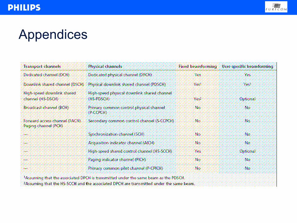
Appendices

common and dedicated pilot-based channel · pdf filecommon and dedicated pilot-based channel...

Documents