combinatorial route to algebra: the art of composition ... · the paper is written as a...
TRANSCRIPT
HAL Id: hal-00994980https://hal.inria.fr/hal-00994980
Submitted on 22 May 2014
HAL is a multi-disciplinary open accessarchive for the deposit and dissemination of sci-entific research documents, whether they are pub-lished or not. The documents may come fromteaching and research institutions in France orabroad, or from public or private research centers.
L’archive ouverte pluridisciplinaire HAL, estdestinée au dépôt et à la diffusion de documentsscientifiques de niveau recherche, publiés ou non,émanant des établissements d’enseignement et derecherche français ou étrangers, des laboratoirespublics ou privés.
Combinatorial Route to Algebra: The Art of
CompositionDecomposition
Pawel Blasiak
To cite this version:Pawel Blasiak. Combinatorial Route to Algebra: The Art of Composition
Decomposition. Discrete Mathematics and Theoretical Computer Science, DMTCS, 2009, 12 (2),pp.381-400. <hal-00994980>
Discrete Mathematics and Theoretical Computer Science DMTCS vol. 12:2, 2010, 381–400
Combinatorial Route to Algebra:
The Art of Composition & Decomposition
Pawel Blasiak†
H. Niewodniczanski Institute of Nuclear Physics, Polish Academy of Sciences, Krakow, Poland
received 31st July 2009, revised 23rd March 2010, accepted 10th August 2010.
We consider a general concept of composition and decomposition of objects, and discuss a few natural properties
one may expect from a reasonable choice thereof. It will be demonstrated how this leads to multiplication and co-
multiplication laws, thereby providing a generic scheme furnishing combinatorial classes with an algebraic structure.
The paper is meant as a gentle introduction to the concepts of composition and decomposition with the emphasis on
combinatorial origin of the ensuing algebraic constructions.
Keywords: composition/decomposition of objects, multiplication/co-multiplication, combinatorics, algebra
1 Introduction
A great deal of concrete examples of abstract algebraic structures are based on combinatorial construc-
tions. Their advantage comes from simplicity steaming from the use of intuitive notions of enumeration,
composition and decomposition which oftentimes provide insightful interpretations and neat pictorial ar-
guments. In the present paper we are interested in clarifying the concept of composition/decomposition
and the development of a general scheme which would furnish combinatorial objects with an algebraic
structure.
In recent years the subject of combinatorics has grown into maturity. It gained a solid foundation in
terms of combinatorial classes consisting of objects having size, subject to various constructions trans-
forming classes one into another, see e.g. [FS09, BLL98, GJ83]. Here, we will augment this framework
by considering objects which may compose and decompose according to some internal law. This idea
was pioneered by G.-C. Rota who considered monoidal composition rules and introduced the concept
of section coefficients showing how they lead to the co-algebra and bi-algebra structures [JR79]. It was
further given a firm foundation by A. Joyal [Joy81] on the grounds of the theory of species. In the present
paper we discuss this approach from a modern perspective and generalize the concept of composition in
order to give a proper account for indeterminate (non-monoidal) composition laws according to which
two given objects may combine in more than one way. Moreover, we will provide a few natural condi-
tions one might expect from a reasonable composition/decomposition rule, and show how they lead to
†Email: [email protected]
1365–8050 c© 2010 Discrete Mathematics and Theoretical Computer Science (DMTCS), Nancy, France
382 Pawel Blasiak
algebra, co-algebra, bi-algebra and Hopf algebra structures [Bou89, Swe69, Abe80]. Our treatment has
the virtue of a direct scheme translating combinatorial structures into algebraic ones – it only has to be
to checked whether the law of composition/decomposition of objects satisfies certain properties. We note
that these ideas, however implicit in the construction of some instances of bi-algebras, have never been
explicitly exposed in full generality. We will illustrate this framework on three examples of classical
combinatorial structures: words, graphs and trees. For words we will provide three different composi-
tion/decomposition rules leading to the free algebra, symmetric algebra and shuffle algebra (the latter one
with a non-monoidal composition law) [Lot83, Reu93]. In the case of graphs, except of trivial rules lead-
ing to the commutative and co-commutative algebra, we will also describe the Connes-Krimer algebra of
trees [Kre98, CK98]. One can find many other examples of monoidal composition laws in the seminal
paper [JR79]; for instances of non-monoidal rules see e.g. [GL89, BDH+10]. A comprehensive survey of
a recent development of the subject with an eye on combinatorial methods can be found in [Car07].
The paper is written as a self-contained tutorial on the combinatorial concepts of composition and
decomposition explaining how they give rise to algebraic structures. We start in Section 2 by briefly
recalling the notions of multiset and combinatorial class. In Section 3 we precise the notion of composi-
tion/decomposition and discuss a choice of general conditions which lead to the construction of algebraic
structures in Section 4. Finally, in Section 5 we illustrate this general scheme on a few concrete examples.
2 Preliminaries
2.1 Multiset
A basic object of our study is a multiset. It differs from a set by allowing multiple copies of elements and
formally can be defined as a pair (A,m), where A is a set and m : A −→ N>1 is a function counting
multiplicities of elements.(i) For example the multiset {a, a, b, c, c, c} is described by the underlying set
A = {a, b, c} and the multiplicity function m(a) = 2, m(b) = 1 and m(c) = 3. Note that each set is
a multiset with multiplicities of all elements equal to one. It is a usual practice to drop the multiplicity
function m in the denotation of a multiset (A,m) and simply write A as its character should be evident
from the context (in the following we will mainly deal with multisets!). Extension of the conventional
set-theoretical operations to multisets is straightforward by taking into account copies of elements. Ac-
cordingly, the sum of two multisets (A,mA) and (B,mB) is the multiset A ⊎ B = (A ∪ B,mA∪B)where
mA∪B(x) =
mA(x) +mB(x) , x ∈ A ∩B
mA(x) , x ∈ A−B
mB(x) , x ∈ B −A
, (1)
whilst the product is defined as A × B = (A × B,mA×B), where mA×B((a, b)) = mA(a) · mB(b).We note that one should be cautious when comparing multisets and not forget that equality involves the
coincidence of the underlying sets as well as the multiplicities of the corresponding elements. Similarly,
inclusion of multisets (A,mA) ⊂ (B,mB) should be understood as the inclusion of the underlying sets
A ⊂ B with the additional condition mA(x) 6 mB(x) for x ∈ A.
(i) For equivalent definition of a multiset based on the SEQ construction subject to appropriate equivalence relation see [FS09] p. 26.

Combinatorial Route to Algebra:The Art of Composition & Decomposition 383
2.2 Combinatorial class
In the paper we will be concerned with the concept of combinatorial class C which is a denumerable
collection of objects. Usually, it is equipped with the notion of size | · | : C −→ N which counts some
characteristic carried by objects in the class, e.g. the number of elements they are build of. The size
function divides C into disjoint subclasses Cn = {Γ ∈ C : |Γ | = n} composed of objects of size n only.
Clearly, we have C =⋃
n∈N. A typical problem in combinatorial analysis consists in classifying objects
according to the size and counting the number of elements in Cn.
In the sequel we will often use the multiset construction. For a given combinatorial class C it defines
a new class MSET(C) whose objects are multisets of elements taken from C. We note that the size of
Γ ∈ MSET(C) is canonically defined as the sum of sizes of all its elements, i.e. |Γ | =∑
γ∈Γ |γ|.
3 Combinatorial Composition & Decomposition
We will consider a combinatorial class C consisting of objects which can compose and decompose within
the class. In this section we precisely define both concepts and discuss a few natural conditions one might
expect from a reasonable composition/decomposition rule.
3.1 Composition
Fig. 1: Illustration of the concept of composition. Two puzzles may compose in six possible ways, two of which give
the same result (two at the bottom).
Composition of objects in a combinatorial class C is a prescription how from two objects make another
one in the same class. In general, such a rule may be indeterminate that is allow two given objects to
compose in a number of ways. Furthermore, it can happen that some of these various possibilities produce
the same outcome. See Fig. 1 for illustration. Therefore, a complete description of composition should
keep a record of all the options which is conveniently attained by means of the multiset construction. Here
is the formal definition:

384 Pawel Blasiak
Definition 1 (Composition)
For a given combinatorial class C the composition rule is a mapping
◭ : C × C −→ MSET (C) , (2)
assigning to each pair of objects Γ2, Γ1 ∈ C the multiset, denoted by Γ2 ◭ Γ1, consisting of all possible
compositions of Γ2 with Γ1, where multiple copies keep an account of the number of ways in which given
outcome occurs. Sometimes, for brevity we will write (Γ2, Γ1) ❀ Γ ∈ Γ2 ◭ Γ1.
Note that this definition naturally extends to the mapping ◭ : MSET (C) × MSET (C) −→ MSET (C)which for given two multisets Γ2, Γ1 ∈ MSET(C) take their elements one by one, compose and collect
the results all together, i.e.
Γ2 ◭ Γ1 =⊎
γ2∈Γ2,γ1∈Γ1
γ2 ◭ γ1 . (3)
At this point the concept of composition is quite general, and its further development obviously depends
on the choice of the rule. One supplements this construction with additional constraints. Below we discuss
some natural conditions one might expect from a reasonable composition rule.
(C1) Finiteness. It is sensible to assume that objects compose only in a finite number of ways, i.e. for
each Γ2, Γ1 ∈ C we have
# Γ2 ◭ Γ1 <∞ . (4)
(C2) Triple composition. Composition applies to more that two objects as well. For given Γ3, Γ2, Γ1 ∈ Cone can compose them successively and construct the multiset of possible compositions. There are
two possible scenarios however: one can either start by composing the first two (Γ2, Γ1) ❀ Γ ′
and then composing the outcome with the third (Γ3, Γ′) ❀ Γ , or change the order and begin with
(Γ3, Γ2) ❀ Γ ′′ followed by the composition with the first (Γ ′′, Γ1) ❀ Γ . It is plausible to require
that both scenarios lead to the same multiset. This condition is a sort of associativity property which
in a compact form reads
Γ3 ◭ (Γ2 ◭ Γ1) = (Γ3 ◭ Γ2) ◭ Γ1 . (5)
Note that it justifies dropping of the brackets in the denotation of triple composition Γ3 ◭ Γ2 ◭ Γ1.
Clearly, the procedure generalizes to multiple compositions and Eq. (5) entails analogous condition
in this case as well.
(C3) Neutral object. Often, in a class there exists a neutral object, denoted by Ø, which composes with
elements of the class only in a trivial way, i.e. (Ø, Γ ) ❀ Γ and (Γ,Ø) ❀ Γ . In other words, for
each Γ ∈ C we have
Ø ◭ Γ = {Γ} & Γ ◭ Ø = {Γ} . (6)
Note that if Ø exists, it is unique.
(C4) Symmetry. Sometimes the composition rule is such that the order in which elements are composed
is irrelevant. Then for each Γ2, Γ1 ∈ C the following commutativity condition holds
Γ2 ◭ Γ1 = Γ1 ◭ Γ2 . (7)
Combinatorial Route to Algebra:The Art of Composition & Decomposition 385
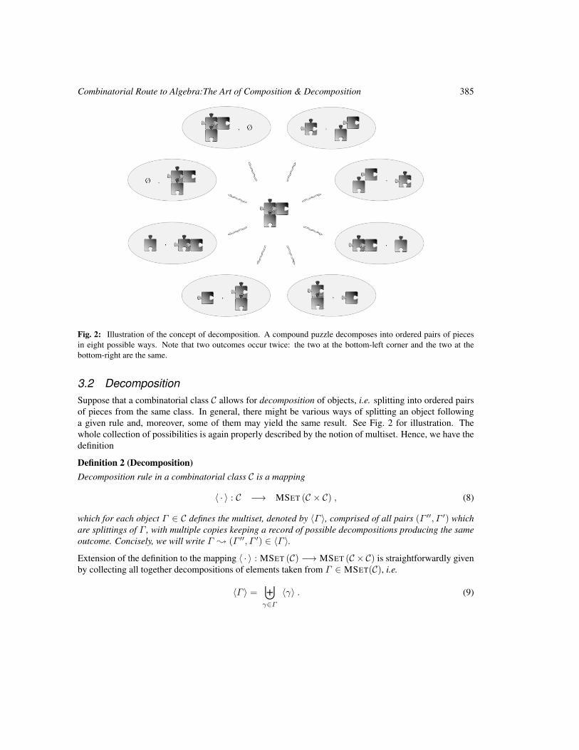
Fig. 2: Illustration of the concept of decomposition. A compound puzzle decomposes into ordered pairs of pieces
in eight possible ways. Note that two outcomes occur twice: the two at the bottom-left corner and the two at the
bottom-right are the same.
3.2 Decomposition
Suppose that a combinatorial class C allows for decomposition of objects, i.e. splitting into ordered pairs
of pieces from the same class. In general, there might be various ways of splitting an object following
a given rule and, moreover, some of them may yield the same result. See Fig. 2 for illustration. The
whole collection of possibilities is again properly described by the notion of multiset. Hence, we have the
definition
Definition 2 (Decomposition)
Decomposition rule in a combinatorial class C is a mapping
〈 · 〉 : C −→ MSET (C × C) , (8)
which for each object Γ ∈ C defines the multiset, denoted by 〈Γ 〉, comprised of all pairs (Γ ′′, Γ ′) which
are splittings of Γ , with multiple copies keeping a record of possible decompositions producing the same
outcome. Concisely, we will write Γ ❀ (Γ ′′, Γ ′) ∈ 〈Γ 〉.
Extension of the definition to the mapping 〈 · 〉 : MSET (C) −→ MSET (C × C) is straightforwardly given
by collecting all together decompositions of elements taken from Γ ∈ MSET(C), i.e.
〈Γ 〉 =⊎
γ∈Γ
〈γ〉 . (9)
386 Pawel Blasiak
Below, analogously as in Section 3.1 we consider some general conditions which one might require
from a reasonable decomposition rule. We observe that most of them are in a sense dual to those discussed
for the composition rule, which reflects the opposite character of both procedures. Note, however, that the
decomposition rule is so far unrelated to composition – insofar as the latter might be even not defined –
and the conditions should be treated as independent.
(D1) Finiteness. One may reasonably expect that objects decompose in a finite number of ways only, i.e.
for each Γ ∈ C we require
# 〈Γ 〉 <∞ . (10)
(D2) Triple decomposition. Decomposition into pairs naturally extends to splitting an object into three
pieces Γ ❀ (Γ3, Γ2, Γ1). An obvious way to carry out the multiple splitting is by applying the
same procedure repeatedly, i.e. decomposing one of the components obtained in the preceding step.
Following this prescription one usually expects that the result does not depend on the choice of the
component it is applied to. In other words, we require that we end up with the same collection of
triple decompositions when splitting Γ ❀ (Γ ′′, Γ1) and then splitting the left component Γ ′′❀
(Γ3, Γ2), as in the case when starting with Γ ❀ (Γ3, Γ′) and then splitting the right component
Γ ′❀ (Γ2, Γ1). This condition can be seen as a sort of co-associativity property for decomposition,
and in explicit form boils down to the following equality between multisets of triple decompositions⊎
(Γ ′′,Γ ′)∈〈Γ 〉
{Γ ′′} × 〈Γ ′〉 =⊎
(Γ ′′,Γ ′)∈〈Γ 〉
〈Γ ′′〉 × {Γ ′} . (11)
The above procedure directly extends to splitting into multiple pieces Γ ❀ (Γn, ...Γ1) by iterated
decomposition. Clearly, the condition of Eq. (11) asserts the same result no matter which way de-
compositions are carried out. Hence, we can consistently define the multiset consisting of multiple
decompositions of an object as
〈Γ 〉(n) =⊎
Γ❀(Γn,...Γ1)
{(Γn, ..., Γ1)} , (12)
with the convention 〈Γ 〉(1) = 〈Γ 〉.
(D3) Void object. Oftentimes, a class contains a void (or empty) element Ø, such that objects decompose
in a trivial way. It should have the property that any object Γ 6= Ø splits into a pair containing either
Ø or Γ in exactly two ways
Γ ❀ (Ø, Γ ) & Γ ❀ (Γ,Ø) , (13)
and Ø ❀ (Ø,Ø). Clearly, if Ø exists, it is unique.
(D4) Symmetry. For some rules the order between components in decompositions is immaterial, i.e. it
allows for the exchange (Γ ′, Γ ′′) ←→ (Γ ′′, Γ ′). In this case we have the following symmetry
condition
(Γ ′, Γ ′′) ∈ 〈Γ 〉 ⇐⇒ (Γ ′′, Γ ′) ∈ 〈Γ 〉 , (14)
and multiplicities of (Γ ′, Γ ′′) and (Γ ′′, Γ ′) in 〈Γ 〉 are the same.

Combinatorial Route to Algebra:The Art of Composition & Decomposition 387
(D5) Finiteness of multiple decompositions. Recall multiple decompositions Γ ❀ (Γn, ...Γ1) consid-
ered in condition (D4) and observe that we may go with the number of components to any n ∈ N.
However, if one takes into account only nontrivial decompositions, i.e. such that do not contain
void Ø components, it is often the case that the process terminates after a finite number of steps. In
other words, for each Γ ∈ C there exists N ∈ N such that for all n > N one has
{Γ ❀ (Γn, ...Γ1) : Γn, ..., Γ1 6= Ø} = ∅ . (15)
3.3 Compatibility
Now, let us take a combinatorial class C which admits both composition and decomposition of objects at
the same time. We give a simple compatibility condition for both procedures to be consistently combined
together.
(CD1) Composition–decomposition compatibility. Suppose we are given a pair of objects (Γ2, Γ1) ∈C × C which we want to decompose. We may think of two consistent decomposition schemes
which involve composition as an intermediate step. We can either start by composing them together
Γ2 ◭ Γ1 and then splitting all the resulting objects into pieces, or first decompose each of them
separately into 〈Γ2〉 and 〈Γ1〉 and then compose elements of both multisets in a component-wise
manner. One may reasonably expect the same outcome no matter which procedure is applied. The
formal description of compatibility comes down to the equality of multisets
〈Γ2 ◭ Γ1〉 =⊎
(Γ ′′
2 ,Γ ′
2)∈〈Γ2〉
(Γ ′′
1 ,Γ ′
1)∈〈Γ1〉
(Γ ′′2 ◭ Γ ′′
1 )× (Γ ′2 ◭ Γ ′
1) . (16)
We remark that this property implies that the void and neutral object of conditions (D3) and (C3)
are the same, and hence common denotation Ø.
Oftentimes, composition/decomposition of objects come alongside with the notion of size. It is usually
the case when their defining rules make use of the same characteristics which are counted by the size
function. Here is a useful condition connecting these concepts:
(CD2) Compatibility with size. It may happen that the considered composition rule preserves size. This
means that when composing two objects (Γ2, Γ1) ❀ Γ sizes of both components add up, i.e.
|Γ | = |Γ2|+ |Γ1| for Γ ∈ Γ2 ◭ Γ1 . (17)
This requirement boils down to the restriction on the mapping of Eq. (2) in the following way:(ii)
◭ : Ci × Cj −→ MSET (Ci+j) . (18)
A parallel condition for decomposition implies that after splitting Γ ❀ (Γ ′′, Γ ′) the original size
of an object distributes between the parts, i.e.
|Γ | = |Γ ′′|+ |Γ ′| for (Γ ′′, Γ ′) ∈ 〈Γ 〉 . (19)
(ii) Recall, that the size function | · | : C −→ N divides C into disjoint subclasses Cn = {Γ ∈ C : |Γ | = n}, such thatC =
⋃n∈N
Cn.

388 Pawel Blasiak
This translates into the constraint on the mapping of Eq. (8) as:
〈 · 〉 : Ck −→ MSET
( ⊎
i+j=k
Ci × Cj)
. (20)
In the following, we will assume that there is a single object of size zero, i.e. C0 = {Ø}.
4 Construction of Algebraic Structures
We will demonstrate the way in which combinatorial objects can be equipped with natural algebraic struc-
tures based on the composition/decomposition concept. The key role in the argument play the conditions
discussed in Section 3 which provide a route to systematic construction of the algebra, co-algebra, bi-
algebra and Hopf algebra structures. We note that most of combinatorial algebras can be systematically
treated along these lines.
4.1 Vector space
For a given combinatorial class C we will consider a vector space C over a field K which consists of
(finite) linear combinations of elements in C, i.e.
C = K C ={ ∑
iαi Γi : αi ∈ K, Γi ∈ C
}
. (21)
Addition of elements and multiplication by scalars in C has the usual form∑
iαi Γi +
∑
iβi Γi =
∑
i(αi + βi) Γi , (22)
α∑
iβi Γi =
∑
i(αβi) Γi . (23)
Clearly, elements of C are independent and span the whole vector space. Hence, C comes endowed
with the distinguished basis which, in addition, carries a combinatorial meaning. We will call C the
combinatorial basis of C .
4.2 Multiplication & co-multiplication
Having defined the vector space C built on a combinatorial class C we are ready to make use of its
combinatorial content. Below we provide a general scheme for constructing an algebra and co-algebra
structures [Bou89] based on the notions of composition and decomposition discussed in Section 3.
Suppose C admits composition as defined in Section 3.1. We will consider a bilinear mapping
∗ : C × C −→ C (24)
defined on basis elements Γ2, Γ1 ∈ C as the sum of all possible compositions of Γ2 with Γ1, i.e.
Γ2 ∗ Γ1 =∑
Γ∈Γ2◭Γ1
Γ . (25)
Note, that although all coefficients in the defining Eq. (25) are equal to one, some of the terms in the sum
may appear several times; this is because Γ2 ◭ Γ1 is a multiset. One rightly anticipates that multiplicities
of elements will play the role of structure constants of the algebra. Such defined mapping is a natural
candidate for multiplication and we have the following statement

Combinatorial Route to Algebra:The Art of Composition & Decomposition 389
Proposition 1 (Algebra)
The vector space C with the multiplication defined in Eq. (25) forms an associative algebra with unit
(C ,+, ∗,Ø) if conditions (C1) – (C3) hold. Under condition (C4) it is commutative.
Proof: Condition (C1) guarantees that the sum in Eq. (25) is finite – hence it is well defined. Conditions
(C3) and (C4) directly translate into the existence of the unit element Ø and commutativity respectively.
Associativity is the consequence of bilinearity of multiplication and condition (C2) which asserts equal-
ity of multisets resulting from two scenarios of triple composition (Γ3, Γ2, Γ1) ❀ Γ ; it is straightforward
to check for basis elements that
Γ3 ∗ (Γ2 ∗ Γ1) =∑
Γ∈Γ3◭Γ2◭Γ1
Γ = (Γ3 ∗ Γ2) ∗ Γ1 . (26)
✷
Now, we will consider C equipped with the notion of decomposition as described in Section 3.2. Let us
take a linear mapping
∆ : C −→ C ⊗ C (27)
defined on basis elements Γ ∈ C as the sum of all splittings into pairs, which in explicit form reads
∆(Γ ) =∑
(Γ ′′,Γ ′)∈〈Γ 〉
Γ ′′ ⊗ Γ ′ . (28)
Repetition of terms in Eq. (28) leads after simplification to coefficients which are multiplicities of elements
in the multiset 〈Γ 〉. These numbers are sometimes called section coefficients, see [JR79]. We will also
need a linear mapping
ε : C −→ K (29)
which extracts the expansion coefficient standing at the void Ø. It is defined on basis elements Γ ∈ C in
a canonical way
ε(Γ ) =
{1 if Γ = Ø ,
0 otherwise .(30)
These mappings play the role of co-multiplication and co-unit in the construction of a co-algebra as
explained in the following proposition
Proposition 2 (Co-algebra)
If conditions (D1) – (D3) are satisfied the mappings ∆ and ε defined in Eqs. (28) and (30) respectively
are the co-multiplication and co-unit which make the vector space C into a co-algebra (C ,+,∆, ε). It is
co-commutative if condition (D4) holds.
390 Pawel Blasiak
Proof: The sum in Eq. (28) is well defined as long as the number of compositions is finite, i.e. condition
(D1) is satisfied. From equivalence of triple splittings Γ ❀ (Γ3, Γ2, Γ1) obtained in two possible ways
considered in condition (D2), one readily verifies for a basis element that
(∆⊗ Id) ◦∆(Γ ) =∑
Γ❀(Γ3,Γ2,Γ1)
Γ3 ⊗ Γ2 ⊗ Γ1 = (Id⊗∆) ◦∆(Γ ) , (31)
which by linearity extends on all C proving co-associativity of co-multiplication defined in Eq. (28).
The co-unit ε : C −→ K by definition should satisfy the equalities
(ε⊗ Id) ◦∆ = Id = (Id⊗ ε) ◦∆ , (32)
where the identification K⊗ C = C ⊗K = C is implied. We will check the first one for a basis element
Γ by direct calculation
(ε⊗ Id) ◦∆(Γ ) =∑
(Γ1,Γ2)∈〈Γ 〉
ε(Γ1)⊗ Γ2 = 1⊗ Γ = Γ = Id (Γ ) . (33)
Note that we have applied condition (D3) by taking all terms in the sum equal to zero except the unique
decomposition (Ø, Γ ) picked up by ε in accordance with the definition of Eq. (30). The identification
1⊗Γ = Γ completes the proof of the first equality in Eq. (32); verification of the second one is analogous.
Check of co-commutativity of the co-product under condition (D4) is immediate.
✷
4.3 Bi-algebra and Hopf algebra structure
We have seen in Propositions 1 and 2 how the notions of composition and decomposition lead to algebra
and co-algebra structure respectively. Both schemes can be combined together so to furnish C with a
bi-algebra structure.
Theorem 1 (Bi-algebra)
If condition (CD1) is satisfied, than the algebra and co-algebra structures in C are compatible and
combine into a bi-algebra (C ,+, ∗,Ø,∆, ε).
Proof: The structure of a bi-algebra requires that the co-multiplication ∆ : C ⊗C −→ C and the co-unit
ε : C −→ K of the co-algebra preserve multiplication in C . Thus, we need to verify for basis elements
Γ1 and Γ2 that
∆(Γ2 ∗ Γ1) = ∆ (Γ2) ∗∆(Γ1) , (34)
with component-wise multiplication in the tensor product G ⊗ G on the right-hand-side, and that
ε (Γ2 ∗ Γ1) = ε (Γ2) ε (Γ1) , (35)
with terms on the right-hand-side multiplied in the field K.
We check Eq. (34) directly by expanding both sides using definitions of Eqs. (25) and (28). Accordingly,
the left-hand-side takes the form
∆(Γ2 ∗ Γ1) =∑
Γ∈Γ2◭Γ1
∆(Γ ) =∑
Γ∈Γ2◭Γ1
(Γ ′′,Γ ′)∈〈Γ 〉
Γ ′′ ⊗ Γ ′ =∑
(Γ ′′,Γ ′)∈〈Γ2◭Γ1〉
Γ ′′ ⊗ Γ ′ , (36)
Combinatorial Route to Algebra:The Art of Composition & Decomposition 391
while the right-hand-side reads
∆(Γ2) ∗∆(Γ1) =∑
(Γ ′′
2 ,Γ ′
2)∈〈Γ2〉
(Γ ′′
1 ,Γ ′
1)∈〈Γ1〉
(Γ ′′2 ⊗ Γ ′
2) ∗ (Γ′′1 ⊗ Γ ′
1)︸ ︷︷ ︸
(Γ ′′
2 ∗Γ ′′
1 )⊗(Γ ′
2∗Γ′
1)
=∑
(Γ ′′
2 ,Γ ′
2)∈〈Γ2〉
(Γ ′′
1 ,Γ ′
1)∈〈Γ1〉
∑
Γ ′′∈Γ ′′
2 ◭Γ ′′
1
Γ ′∈Γ ′
2◭Γ ′
1
Γ ′′ ⊗ Γ ′ . (37)
A closer look at condition (CD1) and Eq. (16) shows a one-to-one correspondence between terms in the
sums on the right-hand-sides of Eqs. (36) and (37), which proves Eq. (34).
Verification of Eq. (35) rests upon a simple observation, steaming from (C3), (D3) and (CD1), that
composition of objects Γ2 ◭ Γ1 yields the neutral element Ø only if both of them are void. Then, both
sides of Eq. (35) are equal to 1 for Γ1 = Γ2 = Ø and 0 otherwise, which ends the proof.
✷
Finally, let us take a linear mapping
S : C −→ C , (38)
defied as an alternating sum of multiple products over possible nontrivial decompositions of an object, i.e.
S(Γ ) =∑
Γ❀(Γn,...,Γ1)Γn,...,Γ1 6= Ø
(−1)n Γn ∗ ... ∗ Γ1 (39)
for Γ 6= Ø and S(Ø) = Ø. This mapping provides an antipode completing the construction of a Hopf
algebra structure on C [Swe69, Abe80].
Proposition 3 (Hopf Algebra)
If furthermore condition (D5) holds, S defined in Eq. (39) is the antipode which makes the bi-algebra C
of Theorem 1 into a Hopf algebra (C ,+, ∗,Ø,∆, ε, S).
Proof:
A Hopf algebra consists of a bi-algebra (C ,+, ∗,Ø,∆, ε) equipped with an antipode S : C −→ C .
The latter is an endomorphism by definition satisfying the property
µ ◦ (Id⊗ S) ◦∆ = ǫ = µ ◦ (S ⊗ Id) ◦∆ , (40)
where for better clarity multiplication was denoted by µ(Γ2⊗Γ1) = Γ2 ∗Γ1. The mapping ǫ : C −→ C ,
defined as ǫ = Ø ε, is the projection on the subspace spanned by Ø, i.e.
ǫ(Γ ) =
{Γ if Γ = Ø ,
0 otherwise .(41)
We will prove that S given in Eq. (39) satisfies the condition of Eq. (40). We start by considering an
auxiliary linear mapping Φ : End(C ) −→ End(C ) defined as
Φ(f) = µ ◦ (Id⊗ f) ◦∆ , for f ∈ End(C ) . (42)
392 Pawel Blasiak
Observe that under the assumption that Φ is invertible the first equality in Eq. (40) can be rephrased into
the condition
S = Φ−1(ǫ) . (43)
Now, our objective is to show that Φ is invertible and calculate its inverse explicitly. By extracting identity
we get Φ = Id+Φ+ and observe that such defined Φ+ can be written in the form
Φ+(f) = µ ◦ (ǫ⊗ f) ◦∆ , for f ∈ End(C ) , (44)
where ǫ = Id− ǫ is the complement of ǫ projecting on the subspace spanned by Γ 6= Ø, i.e.
ǫ(Γ ) =
{0 if Γ = Ø ,
Γ otherwise .(45)
We claim that he mapping Φ is invertible with the inverse given by(iii)
Φ−1 =
∞∑
n=0
(−Φ+)n . (46)
In order to check that the above sum is well defined one analyzes the sum term by term. It is not difficult
to calculate n-th iteration of Φ+ explicitly
(Φ+
)n(f)(Γ ) =
∑
Γ❀(Γk,...,Γ1,Γ0)Γk,...,Γ1 6=Ø
Γk ∗ ... ∗ Γ1 ∗ f(Γ0) . (47)
We note that in the above formula products of multiple decompositions arise from repeated use of the
property of Eq. (34); the exclusion of empty components in the decompositions (except the single one
on the right hand side) comes from the definition of ǫ in Eq. (45). The latter constraint together with
condition (D5) asserts that the number of non-vanishing terms in Eq. (46) is always finite proving that
Φ−1 is well defined. Finally, using Eqs. (46) and (47) one explicitly calculates S from Eq. (43) obtaining
the formula of Eq. (39).
In conclusion, by construction the linear mapping S of Eq. (39) satisfies the first equality in Eq. (40); the
second equality can be checked analogously. Therefore we have proved S to be an antipode thus making
C into a Hopf algebra.
✷
We remark that by a general theory of Hopf algebras, see [Swe69, Abe80], the property of Eq. (40)
implies that S is an anti-morphism and it is unique. Moreover, if C is commutative or co-commutative
S is an involution, i.e. S ◦ S = Id. We should also observe that the definition of the antipode given in
Eq. (39) admits construction by iteration
S(Γ ) = −∑
(Γ ′′,Γ ′)∈〈Γ 〉Γ ′ 6= Ø
S(Γ ′′) ∗ Γ ′ , (48)
(iii) For a linear mapping L = Id + L+ : V −→ V its inverse can be constructed as L−1 =∑∞
n=0(−L+)n provided
the sum is well defined. Indeed, one readily checks that L ◦ L−1 = (Id + L+) ◦∑∞
n=0(−L+)n =
∑∞n=0
(−L+)n +∑∞n=0
(−L+)n+1 = Id, and similarly L−1 ◦ L = Id.

Combinatorial Route to Algebra:The Art of Composition & Decomposition 393
and S(Ø) = Ø.
Finally, whenever composition/decomposition is compatible with the notion of size in class C we have
a grading in the algebra C as explained in the following proposition:
Proposition 4 (Grading)
Suppose we have a bi-algebra structure (C ,+, ∗,Ø,∆, ε) constructed as in Theorem 1. If condition
(CD2) holds, then C is a graded Hopf algebra with grading given by size in C, i.e.
C =⊕
n∈N
Cn , Cn = Span (Cn) , (49)
where Cn = {Γ ∈ C : |Γ | = n}, and
∗ : Ci × Cj −→ Ci+j , ∆ : Ck −→⊕
i+j=k
Ci ⊗ Cj . (50)
Proof: Note, that condition (CD2) implies (D5), and hence C is a Hopf algebra by Theorem 3. Further-
more, condition (CD2) asserts a proper action of ∗ and ∆ on subspaces Cn built of objects of the same
size.
✷
4.4 A special case: Monoid
Let us consider a simplified situation by taking a determinate composition law of the form
◭ : C × C −→ C , (51)
which means that objects compose in a unique way. In other words, for each Γ2, Γ1 ∈ C the multiset
Γ2 ◭ Γ1 of Definition 1 is always a singleton. Observe that conditions (C2) and (C3) are equivalent to
the requirement that (C,◭) is a monoid. We note that the case of a commutative monoid was thoroughly
investigated by S.A. Joni and G.-C. Rota in [JR79] and further developed by A. Joyal [Joy81].
In this context it is convenient to consider collections C ⊂ C such that each element of C can be
constructed as a composition of a finite number of elements from C, i.e.
C = { Γn ◭ ... ◭ Γ1 : Γn, ... , Γ1 ∈ C } . (52)
We call C a generating class if it is the smallest (in the sense of inclusion) subclass of C with this property.
It has the advantage that when establishing a decomposition rule satisfying (CD1) one can specify it on
the generating class C in arbitrary way
〈 · 〉 : C −→ MSET (C × C) , (53)
and then consistently extend it using Eq. (16) to the whole class C by defining
〈Γn ◭ ... ◭ Γ1〉 =⊎
(Γ ′′
n ,Γ ′
n)∈〈Γn〉. . .
(Γ ′′
1 ,Γ ′
1)∈〈Γ1〉
{(Γ ′′n ◭ ... ◭ Γ ′′
1 , Γ ′n ◭ ... ◭ Γ ′
1)} . (54)

394 Pawel Blasiak
We note that from a practical point of view this way of introducing the decomposition rule is very con-
venient as it restricts the the number of objects to be scrutinized to a smaller class C and automatically
guarantees compatibility of composition and decomposition rules, i.e. (CD1) is satisfied by construction.
Moreover, inspection of other properties is usually simpler in this context as well. For example, if compo-
sition preserves size Eq. (17), then it is enough to check Eq. (19) on C and condition (CD2) automatically
holds on the whole C.
There is a canonical way in which decomposition can be introduced in this setting. Namely, one can
define it on the generating elements Γ ∈ C in a primitive way, i.e.
〈Γ 〉 = {(Ø, Γ ), (Γ,Ø)} . (55)
Observe that such defined decomposition rule upon extension via Eq. (54) satisfies all the conditions
(D1) – (D5), which clears the way to the construction of a Hopf algebra. We note that objects having
the property of Eq. (55) are usually called primitive elements, for which we have
∆(Γ ) = Ø⊗ Γ + Γ ⊗ Ø , (56)
S(Γ ) = −Γ . (57)
5 Examples
Here, we will illustrate how the general framework developed in Sections 3 and 4 works in practice. We
give a few examples of combinatorial objects which via composition/decomposition scheme lead to Hopf
algebra structures. For other examples see e.g. [JR79, Car07, GL89, BDH+10].
5.1 Words
Let A = {l1, l2, ..., ln} be a finite set of letters – an alphabet. We will consider a combinatorial class
A consisting of (finite) words built of the alphabet A, i.e. A = A∗ = {Ø, l1, l1l1, l1l2, ... , li1 ... lik , ... }
where Ø is an empty word. Size of a word will be defined as its lengths (number of letters): | li1 ... lik | = k
and |Ø| = 0. Algebraic structure inA can be introduced in a few ways as explained below [Lot83, Reu93].
5.1.1 Free algebra of words
The simplest composition rule for words is given by concatenation, i.e.(iv)
li1 ... lim ◭ lj1 ... ljn = li1 ... lim lj1 ... ljn . (58)
Observe that (A,◭) is a monoid and A is a generating class. We define decomposition of generators
(letters) in the primitive way, i.e.
〈li〉 = {(Ø, li), (li,Ø)} , (59)
and extend it to the whole class A using Eq. (54). One checks that each decomposition of a word comes
down to the choice of a subword which gives the first component of a splitting (the reminder constitutes
the second one), i.e.
〈li1 ... lik〉 =⊎
j1<...<jmjm+1<...<jk
{(lij1 ... lijm , lijm+1... lijk )} (60)
(iv) We adopt the convention that a sequence of letters indexed by the empty set is the empty word Ø.

Combinatorial Route to Algebra:The Art of Composition & Decomposition 395
Note such defined composition/decomposition rule is compatible with size and hence condition (CD2)
holds. Application of the scheme discussed in previous sections provide us with the mappings
li1 ... lim ∗ lj1 ... ljn = li1 ... lim lj1 ... ljn , (61)
∆(li1 ... lik) =∑
j1<...<jmjm+1<...<jk
lij1 ... lijm ⊗ lijm+1... lijk , (62)
ε(li1 ... lik) = 0 , ε(Ø) = 1 , (63)
S(li1 ... lik) = (−1)k lik ... li1 , (64)
which make A into a graded co-commutative Hopf algebra. It is called a free algebra. Note that if the
alphabet consists of more than one letter then multiplication is non-commutative.
In conclusion, we observe that if the alphabet consists of one letter only A = {x}, then the construction
starts from the the class of words P = {Ø, x, xx, xxx, ...} and leads to the algebra of polynomials in one
variable P = K[x] ={∑n
i=0 αi xi : αi ∈ K
}. In this case, we have
xi ∗ xj = xi+j , ∆(xn) =
n∑
i=0
(n
i
)
xi ⊗ xn−i , ε(xn) = δn,0 , S(xn) = (−1)n xn . (65)
5.1.2 Symmetric algebra
Now, let an alphabet A = {l1, l2, ..., ln} be endowed with a linear order l1 < l2 < ... < ln. We will
consider words arranged in a non-decreasing order and define the pertaining class S in the form
S = {li1 ... lin : i1 6 ... 6 in ∈ N} . (66)
In this case, simple concatenation of words is not a legitimate composition rule and one has to amend it
by additional reordering of letters
li1 ... lim ◭ lim+1... lim+n
= liσ(1)... liσ(m+n)
, (67)
where σ is a unique permutation of {1, 2, ...,m + n} such that iσ(1) 6 ... 6 iσ(m+n). Clearly, (S,◭)is a monoid generated by A. The simplest choice of primitive decomposition for the generators 〈li〉 ={(Ø, li), (li,Ø)} extends to the whole class as follows
〈li1 ... lik〉 =⊎
j1<...<jmjm+1<...<jk
{(lij1 ... lijm , lijm+1... lijk )} (68)
Observe apparent similarity of Eqs. (58) and (60) to Eqs. (67) and (68), with the only difference that words
in the latter two are ordered. Construction of the symmetric algebra S follows the proposed scheme, and
the mappings
linn ... li11 ∗ ljnn ... lj11 = lin+jn
n ... li1+j11 , (69)

396 Pawel Blasiak
∆(li1 ... lik) =∑
j1<...<jmjm+1<...<jk
lij1 ... lijm ⊗ lijm+1... lijk , (70)
ε(li1 ... lik) = 0 , ε(Ø) = 1 , (71)
S(li1 ... lik) = (−1)k li1 ... lik , (72)
define a graded Hopf algebra structure which is both commutative and co-commutative. Note that in
Eq. (69) the repeating letters were grouped together and denoted as powers. As a byproduct of this notation
one immediately observes that the symmetric algebra S is isomorphic to the algebra of polynomials in
many commuting variables K[x1, ..., xn].
5.1.3 Shuffle algebra
We will consider the class of words A and define composition as any shuffle which mixes letters of the
words preserving their relative order. For example, for two words ”shuffle” and ”mix”: ”shmiufxfle”
and ”mixshuffle” are allowed compositions whilst ”shufflemxi” is not. Note that there are always several
possible shuffles for given two (nonempty) words, and hence the use of multiset construction in definition
of the composition rule
li1 ... lim ◭ lim+1 ... lim+n=
⊎
σ(1)<...<σ(m)σ(m+1)<...<σ(m+n)
{liσ(1)... liσ(m)
liσ(m+1)... liσ(m+n)
} , (73)
where the index set runs over all permutations σ of the set {1, 2, ...,m + n} which preserve the relative
order of 1, 2, ...,m and m+1,m+2, ...m+n respectively. One checks that a compatible decomposition
rule is given by cutting a word into two parts and exchanging the prefix with the suffix, i.e.
〈li1 ... lik〉 =⊎
j=0,...,k
{(lij+1 ... lik , li1 ... lij )} . (74)
Note that this is the instance of a non-monoidal composition law. Following the scheme of Section 4 we
arrive at the Hopf algebra structure given by the mappings
li1 ... lim ∗ li1 ... lin =∑
σ(1)<...<σ(m)σ(m+1)<...<σ(m+n)
liσ(1)... liσ(m)
liσ(m+1)... liσ(m+n)
, (75)
∆(li1 ... lik) =k∑
j=0
lij+1... lik ⊗ li1 ... lij , (76)
ε(li1 ... lik) = 0 , ε(Ø) = 1 , (77)
S(li1 ... lik) = (−1)k lik ... li1 , S(Ø) = Ø . (78)
We remark that for such constructed Shuffle algebra the multiplication of Eq. (75) is commutative and the
co-product of Eq. (76) is not co-commutative.
Combinatorial Route to Algebra:The Art of Composition & Decomposition 397
5.2 Graphs
Let us consider a class of undirected graphs G which one graphically represents as a collection of vertices
connected by edges (we exclude isolated vertices). More formally a graph is defined as a mapping Γ :E −→ V (2) prescribing how the edges E are attached to vertices V , where V (2) is a set of unordered
pairs of vertices (not necessarily distinct); for a rigorous definition see [Ore90, Wil96, Die05]. Let the
size of a graph be the number of its edges |Γ | = |E|.
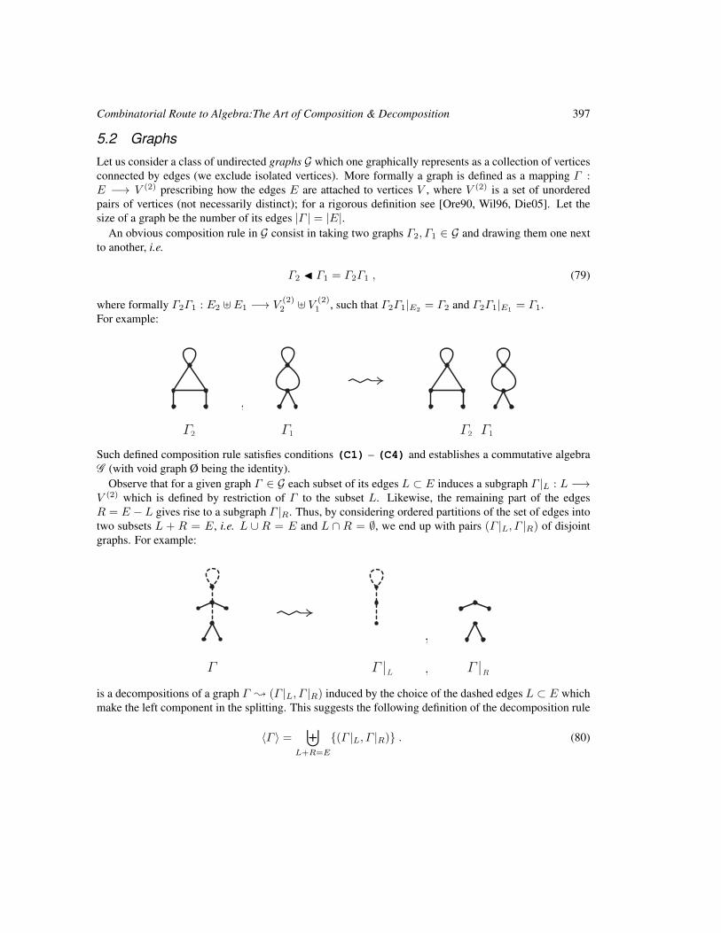
An obvious composition rule in G consist in taking two graphs Γ2, Γ1 ∈ G and drawing them one next
to another, i.e.
Γ2 ◭ Γ1 = Γ2Γ1 , (79)
where formally Γ2Γ1 : E2 ⊎ E1 −→ V(2)2 ⊎ V
(2)1 , such that Γ2Γ1|E2 = Γ2 and Γ2Γ1|E1 = Γ1.
For example:
Such defined composition rule satisfies conditions (C1) – (C4) and establishes a commutative algebra
G (with void graph Ø being the identity).
Observe that for a given graph Γ ∈ G each subset of its edges L ⊂ E induces a subgraph Γ |L : L −→V (2) which is defined by restriction of Γ to the subset L. Likewise, the remaining part of the edges
R = E − L gives rise to a subgraph Γ |R. Thus, by considering ordered partitions of the set of edges into
two subsets L + R = E, i.e. L ∪ R = E and L ∩ R = ∅, we end up with pairs (Γ |L, Γ |R) of disjoint
graphs. For example:
is a decompositions of a graph Γ ❀ (Γ |L, Γ |R) induced by the choice of the dashed edges L ⊂ E which
make the left component in the splitting. This suggests the following definition of the decomposition rule
〈Γ 〉 =⊎
L+R=E
{(Γ |L, Γ |R)} . (80)

398 Pawel Blasiak
One checks that conditions (D1) – (D5) and (CD2) hold, and we obtain a graded Hopf algebra G with
the grading given by the number of edges. Its structure is given by
Γ2 ∗ Γ1 = Γ2Γ1 , (81)
∆(Γ ) =∑
L+R=E
Γ |L ⊗ Γ |R , (82)
ε(Γ ) = 0 , ε(Ø) = 1 , (83)
S(Γ ) =∑
L1+...+Ln=EL1,...,Ln 6= Ø
(−1)n Γ |L1... Γ |Ln
, S(Ø) = Ø . (84)
So defined algebra of graphs is both commutative and co-commutative.
5.3 Trees and Forests
A rooted tree is a graph without cycles with one distinguished vertex, called the root. Let T denote the
class of rooted trees. A forest is a collection of rooted trees and the pertaining combinatorial class has the
specification F = MSET(T ). Size of a tree (forest) is defined as the number of vertices.
We will consider class F and define composition of forests as a multiset union (like for graphs), i.e.
Γ2 ◭ Γ1 = Γ2Γ1 . (85)
For example:
Note that (F ,◮) is a (commutative) monoid generated by the rooted trees T .
For a given a tree τ ∈ T one distinguishes subtrees τ r ⊂ τ which share the same root with τ , called
proper subtrees (the empty tree Ø is considered as a proper subtree as well). Observe that the latter obtains
by trimming τ to the required shape τ r, and the branches which are cut off form a forest of trees denoted
by τ c (with the roots next to the cutting). Decomposition of a tree is defined as any splitting τ ❀ (τ c, τ r)into a pair consisting of a proper subtree taken in the second component and the remaining forest in the
first one. In other words
〈τ〉 =⊎
τr⊂τ
{(τ c, τ r)} , (86)
where the disjoint union ranges over proper subtrees τ r of τ , and τ c is a forest of trees which ’comple-
ments’ τ r to τ . For example:
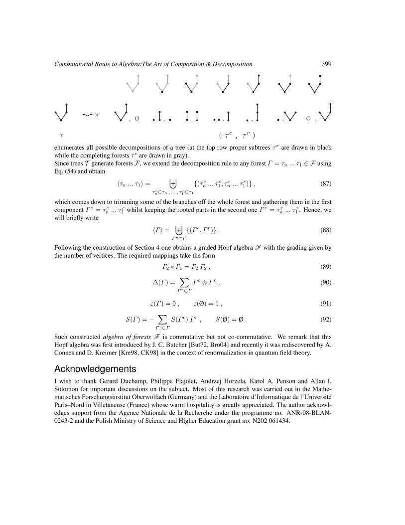
Combinatorial Route to Algebra:The Art of Composition & Decomposition 399
enumerates all possible decompositions of a tree (at the top row proper subtrees τ r are drawn in black
while the completing forests τ c are drawn in gray).
Since trees T generate forests F , we extend the decomposition rule to any forest Γ = τn ... τ1 ∈ F using
Eq. (54) and obtain
〈τn ... τ1〉 =⊎
τrn⊂τn , ... , τr
1⊂τ1
{(τ cn ... τ c1 , τrn ... τ r1 )} , (87)
which comes down to trimming some of the branches off the whole forest and gathering them in the first
component Γ c = τ cn ... τ c1 whilst keeping the rooted parts in the second one Γ r = τ rn ... τ r1 . Hence, we
will briefly write
〈Γ 〉 =⊎
Γ r⊂Γ
{(Γ c, Γ r)} . (88)
Following the construction of Section 4 one obtains a graded Hopf algebra F with the grading given by
the number of vertices. The required mappings take the form
Γ2 ∗ Γ1 = Γ2 Γ2 , (89)
∆(Γ ) =∑
Γ r⊂Γ
Γ c ⊗ Γ r , (90)
ε(Γ ) = 0 , ε(Ø) = 1 , (91)
S(Γ ) = −∑
Γ r⊂Γ
S(Γ c) Γ r , S(Ø) = Ø . (92)
Such constructed algebra of forests F is commutative but not co-commutative. We remark that this
Hopf algebra was first introduced by J. C. Butcher [But72, Bro04] and recently it was rediscovered by A.
Connes and D. Kreimer [Kre98, CK98] in the context of renormalization in quantum field theory.
AcknowledgementsI wish to thank Gerard Duchamp, Philippe Flajolet, Andrzej Horzela, Karol A. Penson and Allan I.
Solomon for important discussions on the subject. Most of this research was carried out in the Mathe-
matisches Forschungsinstitut Oberwolfach (Germany) and the Laboratoire d’Informatique de l’Universite
Paris–Nord in Villetaneuse (France) whose warm hospitality is greatly appreciated. The author acknowl-
edges support from the Agence Nationale de la Recherche under the programme no. ANR-08-BLAN-
0243-2 and the Polish Ministry of Science and Higher Education grant no. N202 061434.
400 Pawel Blasiak
References
[Abe80] E. Abe. Hopf Algebras. Cambridge University Press, 1980.
[BDH+10] P. Blasiak, G. H. E. Duchamp, A. Horzela, K. A. Penson, and A. I. Solomon. Combinatorial
Algebra for second-quantized Quantum Theory. Adv. Theor. Math. Phys., 14(4), 2010. Article
in Press, arXiv:1001.4964 [math-ph].
[BLL98] F. Bergeron, G. Labelle, and P. Leroux. Combinatorial Species and Tree-like Structures.
Cambridge University Press, 1998.
[Bou89] N. Bourbaki. Algebra I: Chapters 1–3. Springer-Verlag, 1989.
[Bro04] C. Brouder. Trees, Renormalization and Differential Equations differential equations. BIT
Num. Math., 44:425–438, 2004.
[But72] J. C. Butcher. An Algebraic Theory of Integration Methods. Math. Comput., 26:79–106,
1872.
[Car07] P. Cartier. A Primer of Hopf Algebrasrimer of hopf algebras. In Frontiers in Number Theory,
Physics, and Geometry II, pages 537–615. Springer, 2007.
[CK98] A. Connes and D. Kreimer. Hopf Algebras, Renormalization and Noncommutative Geometry.
Commun. Math. Phys., 199:203–242, 1998.
[Die05] R. Diestel. Graph Theory. Springer-Verlag, 3rd edition, 2005.
[FS09] P. Flajolet and R. Sedgewick. Analytic Combinatorics. Cambridge University Press, 2009.
[GJ83] I. P. Goulden and D. M. Jackson. Combinatorial Enumeration. John Wiley & Sons, 1983.
[GL89] R. Grossman and R. G. Larson. Hopf-Algebraic Structure of Families of Trees. J. Algebra,
126(1):184–210, 1989.
[Joy81] A. Joyal. Une theorie combinatoire des series formelles. Adv. Math., 42(1):1–82, 1981.
[JR79] S. A. Joni and G. C. Rota. Coalgebras and Bialgebras in Combinatorics. Stud. Appl. Math.,
61:93–139, 1979.
[Kre98] D. Kreimer. On the Hopf algebra structure of perturbative quantum field theory. Adv. Theor.
Math. Phys., 2:303–334, 1998.
[Lot83] M. Lothaire. Combinatorics on Words. Addison-Wesley, 1983.
[Ore90] O. Ore. Graphs and their Uses. Mathematical Association of America, 2nd edition, 1990.
[Reu93] C. Reutenauer. Free Lie Algebras. Oxford University Press, 1993.
[Swe69] M. E. Sweedler. Hopf Algebras. Benjamin, 1969.
[Wil96] R. J. Wilson. Introduction to Graph Theory. Addison-Wesley, 4th edition, 1996.