HAL Id: hal-00661758https://hal.inria.fr/hal-00661758v2

Submitted on 20 Feb 2013

HAL is a multi-disciplinary open accessarchive for the deposit and dissemination of sci-entific research documents, whether they are pub-lished or not. The documents may come fromteaching and research institutions in France orabroad, or from public or private research centers.

L’archive ouverte pluridisciplinaire HAL, estdestinée au dépôt et à la diffusion de documentsscientifiques de niveau recherche, publiés ou non,émanant des établissements d’enseignement et derecherche français ou étrangers, des laboratoirespublics ou privés.

Column Generation for Extended FormulationsRuslan Sadykov, François Vanderbeck

To cite this version:Ruslan Sadykov, François Vanderbeck. Column Generation for Extended Formula-tions. EURO Journal on Computational Optimization, Springer, 2013, 1 (1-2), pp.81-115.<http://link.springer.com/article/10.1007

Column Generation for Extended Formulations

Ruslan Sadykov (1,2) and François Vanderbeck (2,1)(1) INRIA, project-team RealOpt

(2) Univ. of Bordeaux, Institute of Mathematics (CNRS UMR 5251)

INRIA research report hal-00661758, December 2012

Abstract

Working in an extended variable space allows one to develop tighter reformu-lations for mixed integer programs. However, the size of the extended formulationgrows rapidly too large for a direct treatment by a MIP-solver. Then, one can workwith inner approximations defined and improved by generating dynamically vari-ables and constraints. When the extended formulation stems from subproblems’reformulations, one can implement column generation for the extended formulationusing a Dantzig-Wolfe decomposition paradigm. Pricing subproblem solutions areexpressed in the variables of the extended formulation and added to the current re-stricted version of the extended formulation along with the subproblem constraintsthat are active for the subproblem solutions. This so-called “column-and-row gen-eration” procedure is revisited here in a unifying presentation that generalizes thecolumn generation algorithm and extends to the case of working with an approximateextended formulation. The interest of the approach is evaluated numerically on ma-chine scheduling, bin packing, generalized assignment, and multi-echelon lot-sizingproblems. We compare a direct handling of the extended formulation, a standardcolumn generation approach, and the “column-and-row generation” procedure, high-lighting a key benefit of the latter: lifting pricing problem solutions in the space ofthe extended formulation permits their recombination into new subproblem solutionsand results in faster convergence.

Keywords: Extended formulations for MIP, Column-and-Row Generation, Stabilization.

IntroductionFormulating a mixed integer program (MIP) in a higher dimensional space by intro-

ducing extra variables is a process to achieve a tight approximation of the integer convexhull. Several classes of reformulation techniques are reviewed in [29]: some are based onvariable splitting (including multi-commodity flow, unary or binary expansions), othersrely on the existence of a dynamic programming or a linear programming separation pro-cedure for a sub-system, further reformulation techniques rely on exploiting the union ofpolyhedra or basis reduction. A unifying framework is presented in [13]. An extendedformulation presents the practical advantage to lead to a direct approach: the reformu-lation can be fed to a MIP-solver. However, such approach remains limited to small size

1

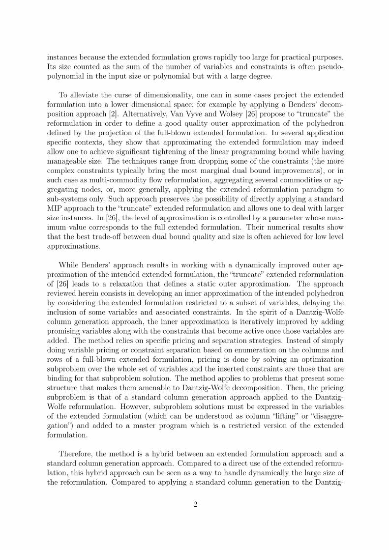
instances because the extended formulation grows rapidly too large for practical purposes.Its size counted as the sum of the number of variables and constraints is often pseudo-polynomial in the input size or polynomial but with a large degree.

To alleviate the curse of dimensionality, one can in some cases project the extendedformulation into a lower dimensional space; for example by applying a Benders’ decom-position approach [2]. Alternatively, Van Vyve and Wolsey [26] propose to “truncate” thereformulation in order to define a good quality outer approximation of the polyhedrondefined by the projection of the full-blown extended formulation. In several applicationspecific contexts, they show that approximating the extended formulation may indeedallow one to achieve significant tightening of the linear programming bound while havingmanageable size. The techniques range from dropping some of the constraints (the morecomplex constraints typically bring the most marginal dual bound improvements), or insuch case as multi-commodity flow reformulation, aggregating several commodities or ag-gregating nodes, or, more generally, applying the extended reformulation paradigm tosub-systems only. Such approach preserves the possibility of directly applying a standardMIP approach to the “truncate” extended reformulation and allows one to deal with largersize instances. In [26], the level of approximation is controlled by a parameter whose max-imum value corresponds to the full extended formulation. Their numerical results showthat the best trade-off between dual bound quality and size is often achieved for low levelapproximations.

While Benders’ approach results in working with a dynamically improved outer ap-proximation of the intended extended formulation, the “truncate” extended reformulationof [26] leads to a relaxation that defines a static outer approximation. The approachreviewed herein consists in developing an inner approximation of the intended polyhedronby considering the extended formulation restricted to a subset of variables, delaying theinclusion of some variables and associated constraints. In the spirit of a Dantzig-Wolfecolumn generation approach, the inner approximation is iteratively improved by addingpromising variables along with the constraints that become active once those variables areadded. The method relies on specific pricing and separation strategies. Instead of simplydoing variable pricing or constraint separation based on enumeration on the columns androws of a full-blown extended formulation, pricing is done by solving an optimizationsubproblem over the whole set of variables and the inserted constraints are those that arebinding for that subproblem solution. The method applies to problems that present somestructure that makes them amenable to Dantzig-Wolfe decomposition. Then, the pricingsubproblem is that of a standard column generation approach applied to the Dantzig-Wolfe reformulation. However, subproblem solutions must be expressed in the variablesof the extended formulation (which can be understood as column “lifting” or “disaggre-gation”) and added to a master program which is a restricted version of the extendedformulation.

Therefore, the method is a hybrid between an extended formulation approach and astandard column generation approach. Compared to a direct use of the extended reformu-lation, this hybrid approach can be seen as a way to handle dynamically the large size ofthe reformulation. Compared to applying a standard column generation to the Dantzig-

2

Wolfe reformulation, the hybrid approach has the advantage of an accelerated convergenceof the column generation procedure: “lifting/disaggregating” columns permits their “re-combination” which acts as a stabilization technique for column generation. Moreover, theextended formulation offers a richer model in which to define cuts or branching restrictions.

Such column-and-row generation procedure is a technique previously described in theliterature in application specific contexts: for bin packing in [23]; for multi-commodityflow in [15] and in [14] where the method is extended to the context of a Lagrangian De-composition – the resulting methodology is named “Lagrangian pricing”; for the resource-constrained minimum-weight arborescence problem in [9]; for split delivery vehicle routingin [7, 8]; or for network design problems in [8, 10]. The convincing computational resultsof these papers indicate the interest of the method. Although the motivations of thesestudies are mostly application specific, methodological statements made therein are tosome extend generic. Moreover, there are recent efforts to explore this approach further.In a study developed concomitantly to ours, Frangioni and Gendron [11] present a “struc-tured Dantzig-Wolfe decomposition” for which they adapt column generation stabilizationtechniques (from linear penalties to the bundle method). Compared to [11], our genericpresentation, relying on the definition of an extended formulation, assumes slightly lessrestrictive assumptions and extends to approximate extended formulation. In [8], Gen-dreau et al. present a branch-and-price-and-cut algorithm where columns and cuts aregenerated simultaneously; their presentation considers approximate extended formulationbut with a weaker termination condition. In [17], Muter et al. consider what they call a“simultaneous column-and-row generation” approach, but it takes the meaning of a nesteddecomposition, different from the method reviewed here: the subproblem has itself a de-composable structure.

The goal of revisiting the column-and-row generation approach is to emphasize itswide applicability and to highlight its pros and cons with an analysis supported by nu-merical experiments. Our paper establishes the validity of the column-and-row generationalgorithm in a form that encompasses all special cases of the literature, completing thepresentations of [8, 9, 10, 11, 14, 15, 17, 23]. We identify what explains the faster con-vergence: the recombination of previously generated subproblem solutions. We point outthat lifting the master program in the variable space of the extended formulation canbe done while carrying pricing in the compact variable space of the original formulation,using any oracle. We show that the method extends to the case where the extendedformulation is based on a subproblem reformulation that only defines an approximationof the subproblem integer hull. This extension is essential in practice as it allows oneto use approximations for strongly NP-Hard subproblems for which an exact extendedformulation is necessarily exponential (unless P=NP). Moreover, we advocate the use ofa generalized termination condition in place of the traditional reduced cost criteria, thatcan lead to stronger dual bounds: solving the integer subproblems yields Lagrangian dualbounds that might be tighter than the extended formulation LP bound. The benefit of theapproach depends on the tradeoff between the induced stabilization effect on one hand,and the larger size working formulation and possible weaker dual bound on the otherhand. Our analysis should help research fellows to evaluate whether this alternative pro-cedure has potential to outperform classical column generation on a particular problem.

3

In the sequel, we introduce (in Section 1) the column-and-row generation method onspecific applications where it has been used, or could have been used. Next, in Section 2,we formalize the procedure and show the validity of the algorithm (including in the caseof multiple identical subproblems). We then show how the method extends to the casewhere one works with an approximate extended formulation (as in the proposal of [26]).We show that in such case, the dual bound that one obtains is between the linear re-laxation bound for the extended reformulation and the Lagrangian dual bound based onthat subproblem. In Section 3, we discuss the pros and cons of the method, we formalizethe lifting procedure, and we highlight the properties that are required for the applica-tion in order to find some specific interest in replacing standard column generation bysuch dynamic column-and-row generation for an extended formulation. This discussionis corroborated by numerical results presented in Section 4. We carry out experimentson machine scheduling, bin packing, generalized assignment, and multi-echelon lot-sizingproblems. We compare a direct solution of the extended formulation linear relaxation,a standard column generation approach for the Dantzig-Wolfe master program, and thecolumn-and-row generation approach applied to the extended formulation LP. The resultsillustrate the stabilization effect resulting from column disaggregation and recombinationsthat is shown to have a cumulative effect when used in combination with a standard sta-bilization technique.

1. Specific Examples

1.1 Machine Scheduling

For scheduling problems, time-indexed formulations are standard extensions result-ing from a unary decomposition of the start time variables. Consider a single machinescheduling problem on a planning horizon T as studied by van den Akker et al. [25]. Theproblem is to schedule the jobs, j ∈ J = {1, . . . , n}, a single one at the time, at minimumcost, which can be modeled as:

[F ] ≡ min{∑j

c(Sj) : Sj + pj ≤ Si or Si + pi ≤ Sj ∀(i, j) ∈ J × J} (1)

where Sj denotes the start time of job j and pj is its given processing time. Disjunctiveprogram (1) admits an extended formulation written in terms of decision variables zjt = 1if and only if job j ∈ J∪{0} starts at the outset of period t ∈ {1, . . . , T}, where job 0 withprocessing time 1 models machine idle time. By convention, period t is associated withtime interval [t − 1, t) and zjt is only defined for 1 ≤ t ≤ T − pj + 1. The reformulation

4

takes the form:

[R] ≡ min∑j∈J

∑t

cjt zjt (2)

T−pj+1∑t=1

zjt = 1 ∀j ∈ J (3)∑j∈J

zj1 = 1 (4)∑j∈J

zjt =∑

j∈J : t−pj≥1

zj,t−pj ∀t > 1 (5)

zjt ∈ {0, 1} ∀j, t (6)

where (3) enforces the assignment of each job, (4) the initialization of the schedule, while(5) forbids the use of the machine for more than one job at the time: a job j can startin t only if one ends in t and therefore releases the machine. The formulation can beextended to the case in which m identical machines are available; then the right-hand-sizeof (4) is m and variable z0t represents the number of idle machines at time t. One canalso model in this way a machine with arbitrary capacity where jobs have unit capacityconsumption. Non overlapping are equivalently modeled as

∑j

∑tτ=t−pj+1 zjτ ≤ 1 ∀t

which define a consecutive one matrix: each variable zjt appears with a 1 in constraintsassociated to consecutive periods t. Hence, this subsystem is totally uni-modular (TU)and can be reformulated as a shortest path. The objective can model any cost functionthat depends on job start times (or completion times). Extended reformulation [R] hassize O(|J |T ) which is pseudo-polynomial in the input size, since T is not an input butit is computed as T =

∑j pj. The subsystem defined by constraints (4-5) characterizes

a flow that represents a “pseudo-schedule” satisfying non-overlapping constraints but notthe single assignment constraints. A standard column generation approach based onsubsystem (4-5) consists in defining reformulation:

[M ] ≡ min{∑g∈G

cg λg :∑g∈G

T−pj+1∑t=1

zgjt λg = 1 ∀j,∑g∈G

λg = m, λg ∈ {0, 1} ∀g ∈ G} (7)

where G is the set of “pseudo-schedules”: vector zg and scalar cg define the associated so-lution and cost for a solution g ∈ G. As done in [24, 25], reformulation [M] can be solvedby column generation. The pricing subproblem [SP] is a shortest path problem: find asequence of jobs and down-times to be scheduled on the single machine with possiblerepetition of jobs. The underlying graph is defined by nodes that represent periods andarcs (t, t+pj) associated to the processing of jobs j ∈ J∪{0} in time interval [t−1, t+pj).Figure 1 illustrates such path for a numerical instance.

An alternative to the above standard column generation approach for [M] would be togenerate dynamically the z variables for [R], not one at the time, but by solving the short-est path pricing problem [SP] and by adding to [R] the components of the subproblemsolution zg in the time index formulation along with the flow conservation constraints thatare binding for that solution. To illustrate the difference between the two approaches,

5

Figure 1: Consider the machine scheduling subproblem. A solution is a pseudo-schedulethat can be represented by a path as illustrated here for T = 10 and J = {1, . . . , 4}and pj = j for each j ∈ J : the sequence consists in scheduling job 3, then twice job 2consecutively, and to complete the schedule with idle periods (represented by straight arcs).

1 2 3 4 5 6 7 8 9 10 11

Figure 2 shows several iterations of the column generation procedure for [M] and [R],for the numerical instance of Figure 1. Formulations [M] and [R] are initialized withthe variable(s) associated to the same pseudo-schedule depicted in Figure 2 as the ini-tial subproblem solution. Note that the final solution of [M] is the solution obtained asthe subproblem solution generated at iteration 11; while, for formulation [R], the final so-lution is a recombination of the subproblem solution of iteration 3 and the initial solution.

As illustrated by the numerical example of Figure 2, the interest of implementingcolumn generation for [R] instead of [M] is to allow for the recombination of previouslygenerated solutions. Observe the final solution of [R] in Figure 2. Let us denote it byz. It would not have its equivalent in formulation [M] even if the same four subproblemsolutions had been generated: zg, for g = 0, . . . , 3. Indeed, if z =

∑3g=0 z

g λg, then λ0 > 0and job 2 must be at least partially scheduled in period 2.

In van den Akker et al. [25] the extended formulation [R] is presented as being typicallytoo large for practical computation purposes. On this ground, the authors make use ofa standard column generation for [M]. But they did not experiment with the alternativeapproach that consists in developing a column generation approach for [R]. Note thata similar alternative to the standard column generation approach has been proposedby Bigras et al. [3]. They split the time horizon into intervals, and solve the pricingsubproblem separately for each interval. This idea improves a lot the convergence ofcolumn generation and its solution time. A disadvantage of this approach is that thecolumns can contain parts of jobs (which span two or more intervals). Thus, in the solutionof the LP relaxation, jobs can be preempted, which results in worse lower bound.

1.2 Bin Packing

A column-and-row generation approach for an extended formulation has been appliedto the bin packing problem by Valerio de Carvalho [23]. The bin packing problem consistsin assigning n items, i ∈ I = {1, . . . , n}, of given size si, to bins of identical capacity C,

6

Figure 2: Solving the example by column versus column-and-row generation (assumingthe same data as in of Figure 1). Each bended arc represents a job, and straight arcsrepresent idle periods.

Iteration Subproblem solution

Initial solution

· · · · · ·

Final solution

Column generation for [M]

1

2

3

10

11

Column-and-rowgeneration for [R]

Subproblem solution

using a minimum number of bins. A compact formulation is:

[F ] ≡ min∑k

δk (8)∑k

xik = 1 ∀i (9)∑i

si xik ≤ C δk ∀k (10)

xik ∈ {0, 1} ∀i, k (11)δk ∈ {0, 1} ∀k (12)

where xik = 1 if item i ∈ I is assigned to bin k for k = 1, . . . , n and δk = 1 if bin k is used.Constraints (9) say that each item must be assigned to one bin, while constraints (10-12)define a knapsack subproblem for each bin k. The standard column generation approachconsists in reformulating the problem in terms of the knapsack subproblem solutions. The

7

master program takes the form:

[M ] ≡ min∑g

λg (13)∑g

xgiλg = 1 ∀i ∈ I (14)

λg ∈ {0, 1} ∀g ∈ G (15)

where G denotes the set of “feasible packings” satisfying (10-12) and vector xg defines theassociated solution g ∈ G. When solving its linear relaxation by column generation, thepricing problem takes the form:

[SP ] ≡ min{δ −∑i

πixi : (x, δ) ∈ X} (16)

where π are dual variables associated to (14) and

X = {(xg, δg)}g∈G = {(x, δ) ∈ {0, 1}n+1 :∑i

sixi ≤ C δ}.

The subproblem can be set as the search for a shortest path in an acyclic network cor-responding to the decision graph that underlies a dynamic programming solution of theknapsack subproblem: the nodes v ∈ {0, . . . , C} are associated with capacity consump-tion levels; each item, i ∈ I, gives rise to arcs (u, v), with v = u+ si; wasted bin capacityis modeled by arcs (v, C) for v = 0, . . . , C − 1. A numerical example is given on the leftof Figure 3.

Figure 3: Knapsack network for C = 6, n = 3, and s = (1, 2, 3)

60 1 2 3 4 5 60 1 2 3 4 5

The network flow model for the subproblem yields an extended formulation for thesubproblem in terms of variables f iuv = 1 if item i is in the bin in position u to v = u+ si.The subproblem reformulation takes the form:

{(f, δ) ∈ {0, 1}n·C+1 :∑i,v

f i0v + f0C = δ (17)∑i,u

f iuv =∑i,u

f ivu + fv,C v = 1, . . . , C − 1 (18)∑i,u

f iuC +∑v

fvC = δ (19)

0 ≤ f iuv ≤ 1 ∀i, u, v = u+ si } (20)

8

(Superscript i is redundant, but it shall help to simplify the notation below.)

Subproblem extended formulation (17-20) leads in turn to an extended formulationfor the original problem in terms of aggregate arc flow variables over all subproblemsassociated with each bin k = 1, . . . , n: F i

uv =∑

k fikuv, FvC =

∑k f

kvC , and ∆ =

∑k δ

k.The extended formulation takes the form:

[R] ≡ min ∆ (21)∑(u,v)

F iuv = 1 ∀i (22)

∑i,v

F i0v + F0C = ∆ (23)∑i,u

F iuv =

∑i,u

F ivu + FvC v = 1, . . . , C − 1 (24)∑

i,u

F iuC +

∑v

FvC = ∆ (25)

F iuv ∈ {0, 1} ∀i, (u, v) : v = u+ si . (26)

Valerio de Carvalho [23] proposed to solve the linear relaxation of (21-26) by col-umn generation: iteratively solve a partial formulation stemming from a restricted set ofvariables F i

uv, collect the dual solution π associated to (22), solve pricing problem (16),transform its solution, x∗, into a path flow that can be decomposed into a flow on thearcs, a solution to (17-20) which we denote by f(x∗), and add in (21-26) the missing arcflow variables {F i

vu : f ivu(x∗) > 0}, along with the missing flow balance constraints active

for f(x∗).

Observe that (17-20) is only an approximation of the extended network flow formula-tion associated to the dynamic programming recursion to solve a 0-1 knapsack problem.A dynamic programming recursion for the bounded knapsack problem yields state space{(j, b) : j = 0, . . . , n; b = 0, . . . , C}, where (j, b) represents the state of a knapsack filledup to level b with a combination of items i ∈ {1, . . . , j}. Here, it has been aggregatedinto state space: {(b) : b = 0, . . . , C}. This entails relaxing the subproblem to an un-bounded knapsack problem. Hence, feasible solutions to (17-20) can involve multiplecopies of the same item. Because (17-20) models only a relaxation of the 0-1 knapsacksubproblem, the LP relaxation of (21-26) is weaker than that of the standard masterprogram (13-15). For instance, consider the numerical example with C = 100, n = 5and s = (51, 50, 34, 33, 18). Then, the LP value of (13-15) is 2.5, while in (21-26) thereis a feasible LP solution of value 2 which is F 1

0,51 = 1, F 351,85 = F 5

51,69 = F 569,87 = 1

2,

F 20,50 = F 2

50,100 = 12, F 3

0,34 = F 434,67 = F 4

67,100 = 12. In [23], to avoid symmetries and to

strengthen the extended formulation, arcs associated to an item are only defined if thetail node can be reached with a filling using items larger than si (as in the right part ofFigure 3). Note that our numerical example of a weaker LP solution for [R] does not holdafter such strengthening.

9

1.3 Multi-Commodity Capacitated Network Design

Frangioni and Gendron [10] applied a column-and-row generation technique to a multi-commodity capacitated network design problem. Given a directed graph G = (V,A) andcommodities: k = 1, . . . , K, with a demand dk of flow between origin and destination(ok, tk) ∈ V × V , the problem is to assign an integer number of nominal capacity on eacharc to allow for a feasible routing of traffic for all commodities, while minimizing routingand capacity installation cost. In [10], split flows are allowed and hence flow variables arecontinuous. A formulation is:

[F ] ≡ min∑i,j,k

ckij xkij +

∑ij

fij yij (27)∑j

xkji −∑j

xkij = dki ∀i, k (28)∑k

xkij ≤ uij yij ∀i, j (29)

0 ≤ xkij ≤ dk yij ∀i, j, k (30)

xkij ≥ 0 ∀i, j, k (31)yij ∈ N ∀i, j (32)

where dki = dk if i = ok, dki = −dk if i = tk, and dki = 0 otherwise. Variables xkij denotethe flow of commodity k in arc (i, j) ∈ A. The design variables, yij, consists in selectingan integer number of nominal capacity on each arc (i, j) ∈ A. The problem decomposedinto a continuous knapsack subproblem with varying capacity for each arc (i, j) ∈ A:X ij = {(x, y) ∈ RK

+ × N :∑

k xk ≤ uij y, x

k ≤ dk y ∀k}. An extended formulation forthe subproblem arises from unary disaggregation of the design variables: let ysij = 1 and

xksij = xkij if yij = s for s ∈ {1, . . . , smaxij } with smax

ij =⌈∑

k dk

uij

⌉. Then, the subproblem

associated to arc (i, j) can be reformulated as:

Zij = {(xksij , ysij) ∈ RK×smaxij

+ × {0, 1}smaxij :∑

s

ysij ≤ 1, (s− 1) uij ysij ≤

∑k

xksij ≤ s uij ysij ∀s, xksij ≤ min{dk, s uij} ysij ∀k, s} .

Its continuous relaxation gives the convex hull of its integer solutions and its projectiongives the convex hull of X ij solutions as shown by Croxton, Gendron and Magnanti [5]:reformulation Zij of subproblem X ij can be obtained as the union of polyhedra associatedwith each integer value of yij = s for s = 0, . . . , smax

ij .

10

These subproblem reformulations yields a reformulation for the original problem:

[R] ≡ min∑i,j,k,s

ckij xksij +

∑ijs

fij s ysij (33)∑

js

xksji −∑js

xksij = dki ∀i, k (34)

(s− 1) uij ysij ≤

∑k

xksij ≤ s uij ysij ∀i, j, s (35)

0 ≤ xksij ≤ min{dk, s uij} ysij ∀i, j, k, s (36)∑s

ysij ≤ 1 ∀i, j (37)

ysij ∈ {0, 1} ∀i, j, s . (38)

On the other hand, a Dantzig-Wolfe reformulation can be derived based on subsystemsX ij or equivalently Zij. Let Gij = {(xg, yg)}g∈Gij be the enumerated set of extremesolutions to Zij. A column g is associated with a given capacity installation level σ:ygs = 1 for a given s = σ and zero for s 6= σ while the associated flow vector xgks = 0 fors 6= σ and it defines an extreme LP solution for s = σ. Then, the Dantzig-Wolfe mastertakes the form

[M] ≡ min∑

i,j,s,g∈Gij

(ckij xgks + fij s y

gs) λ

ijg (39)

∑js

∑g∈Gij

xgks λijg −

∑js

∑g∈Gij

xgks λijg = dki ∀i, k (40)

∑g∈Gij

λijg ≤ 1 ∀i, j (41)

λijg ∈ {0, 1} ∀i, j, g ∈ Gij . (42)

When solving [M] by column generation, the pricing problems take the form:

[SP ij] ≡ min{∑ks

ckij xksij +

∑s

fij s ysij : ({xksij }ks, {ysij}s) ∈ Zij} (43)

for each arc (i, j).

Frangioni and Gendron [10] proceeded to solve reformulation [R] by adding dynami-cally the ysij variable and associated xksij variables for a given s at the time; i.e., for each arc(i, j), they include the solution yij = s that arises as the solution of a pricing subproblem(43) over Zij, while a negative reduced cost subproblem solution is found. Constraints(35-36) that are active in the generated pricing problem solutions are added dynamicallyto [R]. In comparison, a standard column generation approach applied to [M] requiresmore iterations to converge as shown experimentally in [11]. This comparative advantageof the approach based of reformulation [R] has an intuitive explanation: in [R] a fixedyij = s, can be “recombined” with any alternative associated extreme subproblem solutionin the x variables. While, when applying column generation in [M], one might need togenerate several columns associated with the same subproblem solution in the y variablesbut different extreme continuous solution in the x variables.

11

1.4 Vehicle Routing with Split Delivery

The vehicle routing problem (VRP) consists in optimizing delivery routes from a de-pot. Consider an undirected graph G = (V ∪ {o}, E), with cost, ce, on the edges e ∈ E.Nodes, i ∈ V , represent customer sites where a quantity of goods di must be delivered,while o denotes the depot. Vehicles, k = 1, . . . , K, of capacity C must be dispatched tocustomers so as to deliver their demand (here we assume di ≤ C ∀i). The number, K,of available vehicles is assumed to be sufficient. In the continuous split delivery variantstudied by Feillet at al. [7], customer demand di can be met through several deliveries,each of which can represent any fraction of the demand.

The problem can be modeled in terms of the following variables: xik = 1 if customeri is visited by vehicle k, yik is the quantity of good delivered to customer i by vehicle k,and zek = 1 if edge e ∈ E is used in the route followed by vehicle k. The formulation is:

[F] ≡ min {∑e,k

ce zek :∑k

xik ≥ 1 ∀i,∑k

yik ≥ di ∀i,∑i

yik ≤ C ∀k, yik ≤ dixik ∀i, k

∑e∈δ(i)

zek = 2 xik ∀i, k,∑e∈δ(S)

xek ≥ 2xik ∀S ⊂ V \ {i}

x ∈ {0, 1}K|V |, y ∈ RK|V |+ , z ∈ {0, 1}K|E|} .

Consider the subproblem associated with vehicle k:

X = {(x, y, z) ∈ {0, 1}|V | × R|V |+ × {0, 1}|E| :

∑i

yi ≤ C, yi ≤ di xi∀i,

∑e∈δ(i)

ze = 2 xi ∀i,∑e∈δ(S)

xe ≥ 2xi ∀S ⊂ V \ {i}}

(the index k does not appear in the subproblem formulation as all vehicles are identical).

Subsystem X can be reformulated in terms of route selection variables. Assume thatR denotes the set of routes starting and returning from the depot. Each route r ∈ R ischaracterized by an indicator vectors: xri = 1 if customer i is visited in route r and zre = 1if edge e is in route r, and a cost cr =

∑e cez

re . The reformulation is:

Z = {(y, µ) ∈ R|V |×|R|+ × {0, 1}|R| :∑i

yir ≤ Cr µr ∀r, yir ≤ di xri µr∀i, r,

∑r

µr = 1}

where Cr = min{C,∑

i dixri}. The subproblem reformulation yields to a reformulation for

the original problem:

[R] ≡ min{∑r∈R

cr µr :∑r

xriµr ≥ 1∀i,∑r

yir ≥ di∀i,∑i

yir ≤ Crµr ∀r, yir ≤ di xri µr∀i, r,

∑r∈R

µr ≤ K, y ∈ R|V |×|R|+ , µ ∈ N|R|}.

12

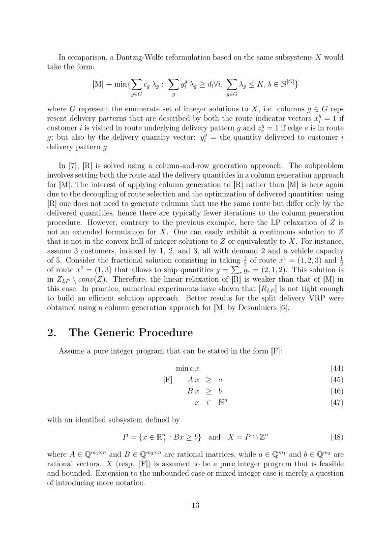
In comparison, a Dantzig-Wolfe reformulation based on the same subsystems X wouldtake the form:

[M] ≡ min{∑g∈G

cg λg :∑g

ygi λg ≥ di∀i,∑g∈G

λg ≤ K,λ ∈ N|G|}

where G represent the enumerate set of integer solutions to X, i.e. columns g ∈ G rep-resent delivery patterns that are described by both the route indicator vectors xgi = 1 ifcustomer i is visited in route underlying delivery pattern g and zge = 1 if edge e is in routeg; but also by the delivery quantity vector: ygi = the quantity delivered to customer idelivery pattern g.

In [7], [R] is solved using a column-and-row generation approach. The subprobleminvolves setting both the route and the delivery quantities in a column generation approachfor [M]. The interest of applying column generation to [R] rather than [M] is here againdue to the decoupling of route selection and the optimization of delivered quantities: using[R] one does not need to generate columns that use the same route but differ only by thedelivered quantities, hence there are typically fewer iterations to the column generationprocedure. However, contrary to the previous example, here the LP relaxation of Z isnot an extended formulation for X. One can easily exhibit a continuous solution to Zthat is not in the convex hull of integer solutions to Z or equivalently to X. For instance,assume 3 customers, indexed by 1, 2, and 3, all with demand 2 and a vehicle capacityof 5. Consider the fractional solution consisting in taking 1

2of route x1 = (1, 2, 3) and 1

2

of route x2 = (1, 3) that allows to ship quantities y =∑

r yr = (2, 1, 2). This solution isin ZLP \ conv(Z). Therefore, the linear relaxation of [R] is weaker than that of [M] inthis case. In practice, numerical experiments have shown that [RLP ] is not tight enoughto build an efficient solution approach. Better results for the split delivery VRP wereobtained using a column generation approach for [M] by Desaulniers [6].

2. The Generic ProcedureAssume a pure integer program that can be stated in the form [F]:

min c x (44)[F] A x ≥ a (45)

B x ≥ b (46)x ∈ Nn (47)

with an identified subsystem defined by

P = {x ∈ Rn+ : Bx ≥ b} and X = P ∩ Zn (48)

where A ∈ Qm1×n and B ∈ Qm2×n are rational matrices, while a ∈ Qm1 and b ∈ Qm2 arerational vectors. X (resp. [F]) is assumed to be a pure integer program that is feasibleand bounded. Extension to the unbounded case or mixed integer case is merely a questionof introducing more notation.

13

Assumption 1 There exists a polyhedron Q = {z ∈ Re+ : H z ≥ h, z ∈ Re

+}, defined bya rational matrix H ∈ Qf×e and a vector h ∈ Qf , and a linear transformation T definingthe projection:

z ∈ Re+ −→ x = (T z) ∈ Rn

+ ;

such that,

(i) Q defines an extended formulation for conv(X), i.e.,

conv(X) = projxQ = {x ∈ Rn+ : x = T z; H z ≥ h; z ∈ Re

+} ;

(ii) Z = Q ∩ Ne defines an extended IP-formulation for X, i.e.,

X = projxZ = {x ∈ Rn+ : x = T z; H z ≥ h; z ∈ Ne} .

Condition (i) is the core of Assumption 1, while condition (ii) is merely a technical restric-tion that simplifies the presentation. It also permits one to define branching restrictionsdirectly in the reformulation. We also assume that Z is bounded to simplify the presen-tation. The dimension e + f of the reformulation is typically much larger than n + m2:while n+m2 (or n at least) is expected to be polynomial in the input size, e+ f can havemuch higher polynomial degree, or even be pseudo-polynomial/exponential in the inputsize.

2.1 Reformulations

The subproblem extended formulation immediately gives rise to a reformulation of [F]to which we refer by [R]:

min c T z (49)[R] A T z ≥ a (50)

H z ≥ h (51)z ∈ Ne . (52)

The standard Dantzig-Wolfe reformulation approach is a special case where X is refor-mulated as:

X = {x =∑g∈G

xgλg :∑g∈G

λg = 1, λg ∈ {0, 1}|G|}, (53)

G defining the set of generators of X (as they are called in [28]), i.e., G is the set of integersolutions of X in the case where X is a bounded pure integer program as assumed here.Then, the reformulation takes a form known as the master program, to which we refer by

14

[M]:

min∑g∈G

c xg λg (54)

[M]∑g∈G

A xg λg ≥ a (55)∑g∈G

λg = 1 (56)

λ ∈ {0, 1}|G| . (57)

Let [RLP ] and [MLP ] denote respectively the linear programming relaxation of [R] and[M], while [D] denote the dual of [MLP ]. Let

vRLP = min{c T z : A T z ≥ a, H z ≥ h, z ∈ Re+} ,

vMLP = min{∑g∈G

c xg λg :∑g∈G

A xg λg ≥ a,∑g∈G

λg = 1, λ ∈ R|G|+ } , and

vDLP = max{π a+ ν : π A xg + ν ≤ c xg ∀g ∈ G, π ∈ Rm1+ , ν ∈ R1} (58)

denote respectively the linear programming (LP) relaxation value of [R], [M], and [D].

Observation 1 Under Assumption 1, the linear programming relaxation optimum valueof both [R] and [M] are equal to the Lagrangian dual value obtained by dualizing constraintsA x ≥ a in formulation [F], i.e.,

vRLP = vMLP = vDLP = v∗ ,

where v∗ := min{cx : A x ≥ a, x ∈ conv(X)}.This is a direct consequence of Assumption 1. Note that the dual bound v∗ obtainedvia such reformulations is often tighter than the linear relaxation value of the originalformulation [F] (as typically conv(X) ⊂ P ).

The above extends easily to the case where subsystem (46) is block diagonal. Then,there are K independent subproblems, one for each block k = 1, . . . , K, with their owngenerator set Gk and associated variables in the reformulation zk, and λkg respectively.When all subsystem are identical, extended reformulation and master are better definedin terms of aggregate variables to avoid symmetries: w =

∑k z

k and λg =∑

k λkg . The

extended formulation becomes

min c T w (59)[AR] A T w ≥ a (60)

H w ≥ h (61)w ∈ Ne (62)

where constraints (61) are obtained by summing over k constraints Hk zk ≥ hk ∀k, as inthe Bin Packing example, when aggregating (17-19) into (23-25). The aggregate mastertakes the form:

[AM ] ≡ min{∑g∈G

c xg λg :∑g∈G

A xg λg ≥ a;∑g∈G

λg = K; λ ∈ N|G|} .

15

Observation 1 remains valid as any solution w to [ARLP ] can be casted into a solutionzk = w

Kfor k = 1, . . . , K to [RLP ]; and any solution λ to [AMLP ] can be casted into a

solution λk = λK

for k = 1, . . . , K to [MLP ].

Given the potential large size of [R], both in terms of number of variables and con-straints, one can solve its LP relaxation using dynamic column-and-row generation. Ifone assumes an explicit description of [R], the standard procedure would be to start offwith a restricted set of variables and constraints (including possibly artificial variablesto ensure feasibility) and to add iteratively negative reduced cost columns and violatedrows by inspection. The alternative hybrid pricing-and-separation strategy consideredhere is to generate columns and rows for [R] not one at the time but by lots, each lotcorresponding to a solution zs of Z (which projects onto xg = Tzs for some g ∈ G) alongwith the constraints (51) that need to be enforced for that solution.

2.2 Restricted Extended Formulation

Let {zs}s∈S be the enumerated set of solutions zs of Z ⊆ Ze+. Then, S ⊂ S, definesan enumerated subset of solutions: {zs}s∈S.Definition 1 Given a solution zs of Z, let J(zs) = {j : zsj > 0} ⊆ {1, . . . , e} be thesupport of solution vector zs and let I(zs) = {i : Hij 6= 0 for some j ∈ J(zs)} ⊆ {1, . . . , f}be the set of constraints of Q that involve some non zero components of zs. The “restrictedreformulation” [R] defined by a subset S ⊂ S of solutions to Z is:

min c T z (63)[R] A T z ≥ a (64)

H z ≥ h (65)

z ∈ N|J | (66)

where z (resp. h) is the restriction of z (resp. h) to the components of J = ∪s∈SJ(zs), His the restriction of H to the rows of I = ∪s∈SI(zs) and the columns of J , while T is therestriction of T to the columns of J .

Assume that we are given a subset S ⊂ S properly chosen to guarantee the feasibilityof [RLP ] (otherwise, artificial variables can be used to patch non-feasibility until set S isexpanded). We define the associated set

G = G(S) = {g ∈ G : xg = T zs for some s ∈ S} (67)

which in turn defines a restricted formulation [M ]. Let [RLP ] and [MLP ] denote the LPrelaxation of the restricted formulations [R] and [M ]; while vRLP , vMLP denote the corre-sponding LP values. Although, in the end, vRLP = vMLP = v∗, as stated in Observation 1,the value of the restricted formulations may differ.

Proposition 1 Let [R] and [M ] be the restricted versions of formulations [R] and [M]both associated to the same subset S ⊂ S of subproblem solutions and associated G asdefined in (67). Under Assumption 1, their linear relaxation values are such that:

v∗ ≤ vRLP ≤ vMLP (68)

16

Proof: The first inequality results from the fact that [RLP ] only includes a subset ofvariables of [R] whose LP value is vRLP = v∗, while the missing constraints are satisfied bythe the current restricted reformulation [RLP ], which we denote by z. More explicitly, allthe missing constraints must be satisfied by the solution that consists in extending z withzero components, i.e. (z, 0) defines a solution to [RLP ]; otherwise, such missing constraintis not satisfied by solutions of S in contradiction with the fact that solutions of S satisfyall constraints of Q. The second inequality is derived from the fact that any solution λ tothe LP relaxation of M has its counterpart z =

∑g∈G z

g λg that defines a valid solutionfor [RLP ], where zg ∈ Z is obtained by lifting solution xg ∈ X. The existence of theassociated zg is guaranteed by Assumption 1-(ii).

The second inequality can be strict: solutions in [RLP ] do not always have theircounterpart in [MLP ] as illustrated in the numerical example of Section 1.1. This is animportant observation that justify considering [R] instead of [M].

2.3 Column Generation

The procedure given in Table 1 is a dynamic column-and-row generation algorithmfor the linear relaxation of [R]. It is a hybrid method that generates columns for [MLP ]by solving a pricing subproblem over X (or equivalently over Z), while getting new dualprices from a restricted version of [RLP ]. Its validity derives from the observations madein Proposition 2.

Proposition 2 Let vRLP denote the optimal LP value of [RLP ], while (π, σ) denote anoptimal dual solution associated to constraints (64) and (65) respectively. Let z∗ be thesubproblem solution obtained in Step 2 of the procedure of Table 1 and ζ = (c− πA) T z∗

be its value. Then:

(i) The Lagrangian bound: L(π) = π a + (c − πA) T z∗ = π a + ζ, defines a valid dualbound for [MLP ], while (π, ζ) defines a feasible solution of [D], the dual of [MLP ].

(ii) Let β denote the best of the above Lagrangian bound encountered in the procedure ofTable 1. If vRLP ≤ β (i.e. when the stopping condition in Step 3 is satisfied), thenv∗ = β and (π, ζ) defines an optimal solution to [D].

(iii) If vRLP > β, then [(c−πA)T −σH]z∗ < 0. Hence, some of the component of z∗ werenot present in [RLP ] and have negative reduced cost for the current dual solution(π, σ).

(iv) Inversely, when [(c − πA) T − σ H]z∗ ≥ 0, i.e., if the generated column has nonnegative aggregate reduced cost for the dual solution of [RLP ], then vRLP ≤ β (thestopping condition of Step 3 must be satisfied) and (π, ν) defines a feasible solutionto formulation [D] defined in (58) for ν = σ h.

Proof:

(i) For any π ≥ 0, and in particular for the current dual solution associated to con-straints (64), L(π) defines a valid Lagrangian dual bound on [F ]. As ζ = min{(c−

17

π A) T z : z ∈ Z} = min{(c− π A) x : x ∈ X}, (π, ζ) defines a feasible solution of[D] and hence its value, π a+ ζ, is a valid dual bound on [MLP ].

(ii) From point (i) and Proposition 1, we have L(π) ≤ β ≤ v∗ ≤ vRLP . When the stoppingcondition in Step 3 is satisfied, the inequalities turn into equalities.

(iii) When vRLP > β ≥ L(π), we note that σ h > (c− π A) Tz∗ because vRLP = π a + σ hand L(π) = π a + ζ = π a + (c − π A) Tz∗. As Hz∗ ≥ h and σ ≥ 0, this impliesthat [(c − π A) T − σ H]z∗ < 0. Assume by contradiction that each component ofz∗ has non negative reduced cost for the current dual solution of [RLP ]. Then, theaggregate sum, [(c−πA)T −σH]z∗ cannot be strictly negative for z∗ ≥ 0. As (π, σ)is an optimal dual solution to [RLP ], all variables of [RLP ] have positive reducedcost. Thus, the negative reduced cost components of z∗ must have been absent from[R].

(iv) Because Hz∗ ≥ h, [(c − πA) T ]z∗ ≥ σ H z∗ implies (c − π A) Tz∗ ≥ σ h, i.e.,ζ ≥ σ h. In turn, ζ ≥ σ h implies that (π, ν) with ν = σ h is feasible for [D] (allconstraints of [D] are satisfied by (π, ν)). Note that ζ ≥ σ h also implies vRLP ≤ β,as vRLP = π a+ σ h ≤ π a+ ζ = L(π) ≤ β.

Table 1: Dynamic column-and-row generation for [RLP ].

Step 0: Initialize the dual bound, β := −∞, and the subproblem solution set S so thatthe linear relaxation of [R] is feasible.

Step 1: Solve the LP relaxation of [R] and record its value vRLP and the dual solution πassociated to constraints (64).

Step 2: Solve the pricing problem: z∗ := argmin{(c − πA) T z : z ∈ Z}, and record itsvalue ζ := (c− πA) T z∗.

Step 3: Compute the Lagrangian dual bound: L(π) := π a + ζ, and update the dualbound β := max{β, L(π)}. If vRLP ≤ β, STOP.

Step 4: Update the current bundle, S, by adding solution zs := z∗ and update theresulting restricted reformulation [R] according to Definition 1. Then, goto Step 1.

Remark 1 The column generation pricing problem of Step 2 in Table 1 is designed forformulation [MLP ] and not for formulation [RLP ]: it ignores dual prices, σ, associated tosubproblem constraints (65).

Remark 2 For the column generation procedure of Table 1, pricing can be operated inthe original variables, x, in Step 2. Indeed, min{(c−πA)T z : z ∈ Z} ≡ min{(c−πA)x :x ∈ X}. But, to implement Step 4, one needs to lift the solution x∗ := argmin{(c−πA)x :x ∈ X} in the z-space in order to add variables to [R], i.e., one must have a procedure todefine z∗ such as x∗ = T z∗.

18

Remark 3 The procedure of Table 1 is a generalization of the standard “text-book” columngeneration algorithm (see f.i. [4]). Applying this procedure to formulation [M] reproducesexactly the standard column generation approach for solving the LP relaxation of [M].Indeed, [M] is a special case of reformulation of type [R] where system H z ≥ h consistsof a single constraint,

∑g∈G λg = 1. The latter needs to be incorporated in the restricted

reformulation along with the first included column, λg, from which point further extensionsconsist only in including further columns.

Observation 2 Note that ν = σ h plays the role of the dual solution associated to theconvexity constraint (56). It defines a valid cut-off value for the pricing sub-problem, i.e.,if ζ ≥ σ h the stopping condition in Step 3 is satisfied.

This observation derives from the proof of Proposition 2-(iv).

2.4 Extension to approximate extended formulations

The column-and-row generation procedure for [R] provided in Table 1 remains validunder weaker conditions. Assumption 1 can be relaxed into:

Assumption 2 Using the notation of Assumption 1, assume:

(i) reformulation Q defines an improved formulation for X, although not an exact ex-tended formulation:

conv(X) ⊂ projxQ ⊂ P where projxQ = {x = T z : H z ≥ h, z ∈ Re+} ;

(ii) moreover, assume conditions (ii) of Assumption 1.

Assumption 2, relaxing Assumption 1-(i), can be more realistic in many applicationswhere the subproblem is strongly NP-Hard. It also applies when one develops only anapproximation of the extended formulation for X as in the proposal of [26] and in thebin-packing example of Section 1.2.

Then, Observation 1 and Proposition 1 become respectively:

Observation 3 Under Assumption 2, vLP ≤ vRLP ≤ v∗ = vMLP = vDLP .

Proposition 3 Under Assumption 2, vRLP ≤ vMLP and v∗ ≤ vMLP ; but one might havevRLP < v∗.

Proposition 2 still holds under Assumption 2 except for point (ii). However the stoppingcondition of Step 3 remains valid.

Proposition 4 Under Assumption 2, the column-and-row generation procedure of Table 1remains valid. In particular, the termination of the procedure remains guaranteed. Ontermination, one may not have the value vRLP of the solution of [RLP ], but one has a validdual bound β that is at least as good, since

vRLP ≤ β ≤ v∗ = vMLP .

19

Proof: Observe that the proofs of points (i), (iii), and (iv) of Proposition 2 remain validunder Assumption 2. Hence, as long as the stopping condition of Step 3 is not satisfied,negative reduced cost columns are found for [RLP ] (as stated in Proposition 2-(iii)) thatshall in turn lead to further decrease of vRLP . Once the stopping condition, vRLP ≤ β, issatisfied however, we have vRLP ≤ vRLP ≤ β ≤ v∗, proving that the optimal LP value, vRLP ,is then guaranteed to lead to a bound weaker than β.

Thus, once vRLP ≤ β, there is no real incentive to further consider columns z∗ withnegative reduced cost components in [RLP ]; although this may decrease vRLP , there is nomore guarantee that β shall increase in further iterations. Note that our purpose is toobtain the best possible dual bound for [F], and solving [RLP ] is not a goal in itself.Nevertheless, sufficient conditions to prove that [RLP ] has been solved to optimality canbe found in [8].

3. Interest of the approachHere, we review the motivations to consider applying column-and-row generation to

[R] instead of a standard column generation to [M] or a direct MIP-solver approach to[R]. We summarize the comparative pros and cons of the hybrid approach. We identifyproperties that are key for the method’s performance and we discuss two generic cases ofreformulations where the desired properties take a special form: reformulations based onnetwork flow models or on the existence of a dynamic programming subproblem solver.

3.1 Pros and cons of a column-and-row generation approach

Both the hybrid column-and-row generation method for [R] and a standard columngeneration approach for [M] can be understood as ways to get around the issue of sizearising in a direct solution of the extended formulation [R]. The primary interest for imple-menting a dynamic generation of [R] rather than [M] is to exploit the second inequality ofProposition 1: a column generation approach to reformulation [RLP ] can converge fasterthan one for [MLP ] when there exist possible re-compositions of solutions in [RLP ] thatwould not be feasible in [MLP ]. In the literature (f.i. in [23]), another motivation is putforward for using the column-and-row generation rather than standard column generation:[R] offers a richer model in which to define cuts or branching restrictions. Note howeverthat although [R] provides new entities for branching or cutting decisions, one can im-plicitly branch or formulate cuts on the variables of [R] while working with [M]: providedone does pricing in the z-space, any additional constraint in the z-variables of the formα z ≥ α0 for [R] translates into a constraint

∑g α z

g λg ≥ α0 for [M] (where zg’s denotegenerators) that can be accommodated in a standard column generation approach for [M].

The drawbacks of a column-and-row approach, compared to applying standard columngeneration, are:

(i) having to handle a larger restricted linear program ([RLP ] has more variables andconstraints than [MLP ] for a given S);

20

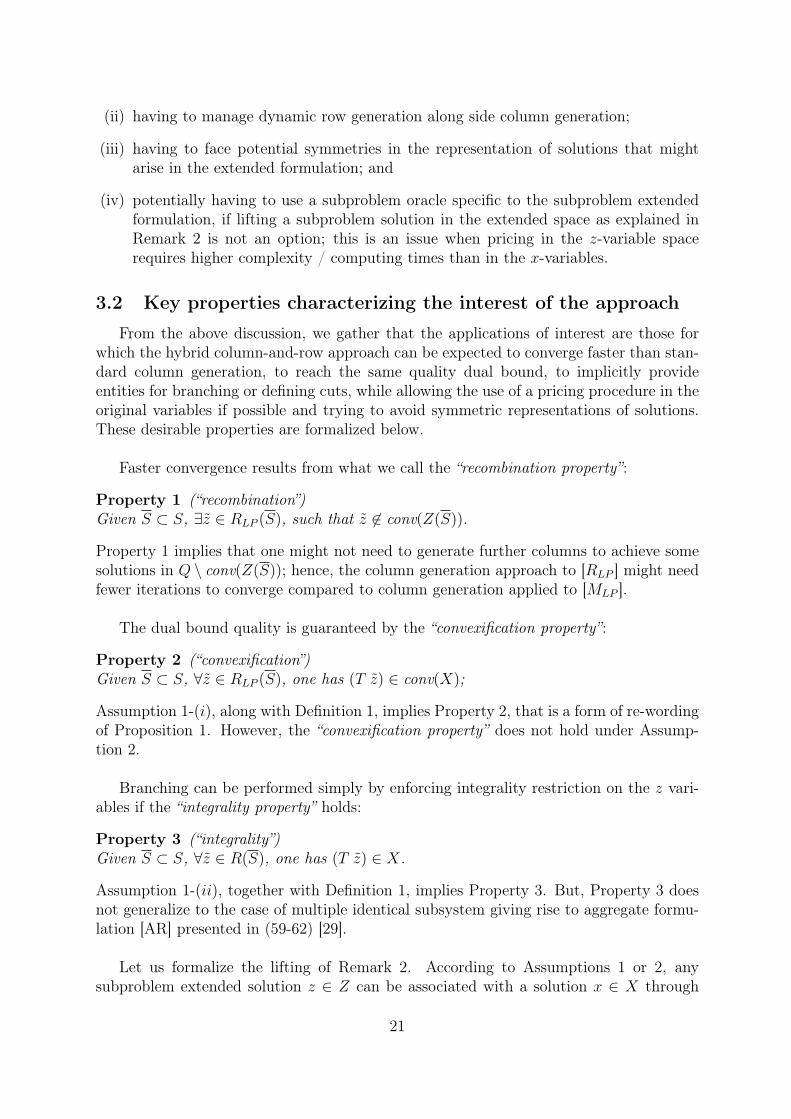
(ii) having to manage dynamic row generation along side column generation;

(iii) having to face potential symmetries in the representation of solutions that mightarise in the extended formulation; and

(iv) potentially having to use a subproblem oracle specific to the subproblem extendedformulation, if lifting a subproblem solution in the extended space as explained inRemark 2 is not an option; this is an issue when pricing in the z-variable spacerequires higher complexity / computing times than in the x-variables.

3.2 Key properties characterizing the interest of the approach

From the above discussion, we gather that the applications of interest are those forwhich the hybrid column-and-row approach can be expected to converge faster than stan-dard column generation, to reach the same quality dual bound, to implicitly provideentities for branching or defining cuts, while allowing the use of a pricing procedure in theoriginal variables if possible and trying to avoid symmetric representations of solutions.These desirable properties are formalized below.

Faster convergence results from what we call the “recombination property”:

Property 1 (“recombination”)Given S ⊂ S, ∃z ∈ RLP (S), such that z 6∈ conv(Z(S)).

Property 1 implies that one might not need to generate further columns to achieve somesolutions in Q \ conv(Z(S)); hence, the column generation approach to [RLP ] might needfewer iterations to converge compared to column generation applied to [MLP ].

The dual bound quality is guaranteed by the “convexification property”:

Property 2 (“convexification”)Given S ⊂ S, ∀z ∈ RLP (S), one has (T z) ∈ conv(X);

Assumption 1-(i), along with Definition 1, implies Property 2, that is a form of re-wordingof Proposition 1. However, the “convexification property” does not hold under Assump-tion 2.

Branching can be performed simply by enforcing integrality restriction on the z vari-ables if the “integrality property” holds:

Property 3 (“integrality”)Given S ⊂ S, ∀z ∈ R(S), one has (T z) ∈ X.

Assumption 1-(ii), together with Definition 1, implies Property 3. But, Property 3 doesnot generalize to the case of multiple identical subsystem giving rise to aggregate formu-lation [AR] presented in (59-62) [29].

Let us formalize the lifting of Remark 2. According to Assumptions 1 or 2, anysubproblem extended solution z ∈ Z can be associated with a solution x ∈ X through

21

the projection operation: x = p(z) = T z. Inversely, given a subproblem solution x ∈ X,the system T z = x must admit a solution z ∈ Z: one can define

p−1(x) := {z ∈ Ne : T z = x; H z ≥ h} . (69)

However, in practice, one needs an explicit operator:

x ∈ X −→ z ∈ p−1(x)

or a procedure that returns z ∈ Z, given x ∈ X. Thus, the desirable property is what wecall the “lifting property”:

Property 4 (“lifting”)There exists a lifting procedure that transforms any subsystem solution x ∈ X into asolution to the extended system z ∈ Z such that x = T z.

Then, in Step 2 of the procedure of Table 1, one computes x∗ := argmin{(c− πA) x : x ∈X}, and in Step 4, one defines z∗ = p−1(x∗).

Observation 4 A generic lifting procedure is to solve the integer feasibility program de-fined in (69).

Note that solving (69) is typically much easier than solving the pricing subproblem, asconstraint T z = x already fixes many z variables. However, in an application specificcontext, one can typically derive a combinatorial procedure for lifting. When the richerspace of z-variables is exploited to derive cutting planes or branching constraints for themaster program, it might induce new bounds or a new cost structure in the Z-subproblemthat cannot be modeled in the X space. Then, pricing must be done in the z-space.

Finally, let us discuss further the symmetry drawback. It is characterized by the factthat the set p−1(xg) defined in (69) is often not limited to a singleton (as for instance inthe bin packing example of Section 1.2, when using the underlying network of the left partof Figure 3). In the lack of uniqueness of the lifted solution, the convergence of the so-lution procedure for [RLP ] can be slowed down by iterating between different alternativerepresentations of the same LP solution. (Note that a branch-and-bound enumerationbased on enforcing integrality of the z variables would also suffer from such symmetry.)The lifting procedure can break such symmetry by adopting a rule to select a specificrepresentative of the symmetry class p−1(xg), or by adding constraints in (69).

In summary, a column generation approach for the extended formulation has any in-terest only when Property 1 holds; while Assumption 1 guarantees Properties 2 and 3.Property 4 is optional but if it holds any pricing oracle on X will do, until cut or branch-ing constraint expressed in the z variable might require to price in the z-space. Thecombination of Property 4 and Property 1, leads to the desirable “disaggregation and re-combination property”. We review below several important special cases where the desireddisaggregation and recombination property holds, along side Properties 2 and 3.

22

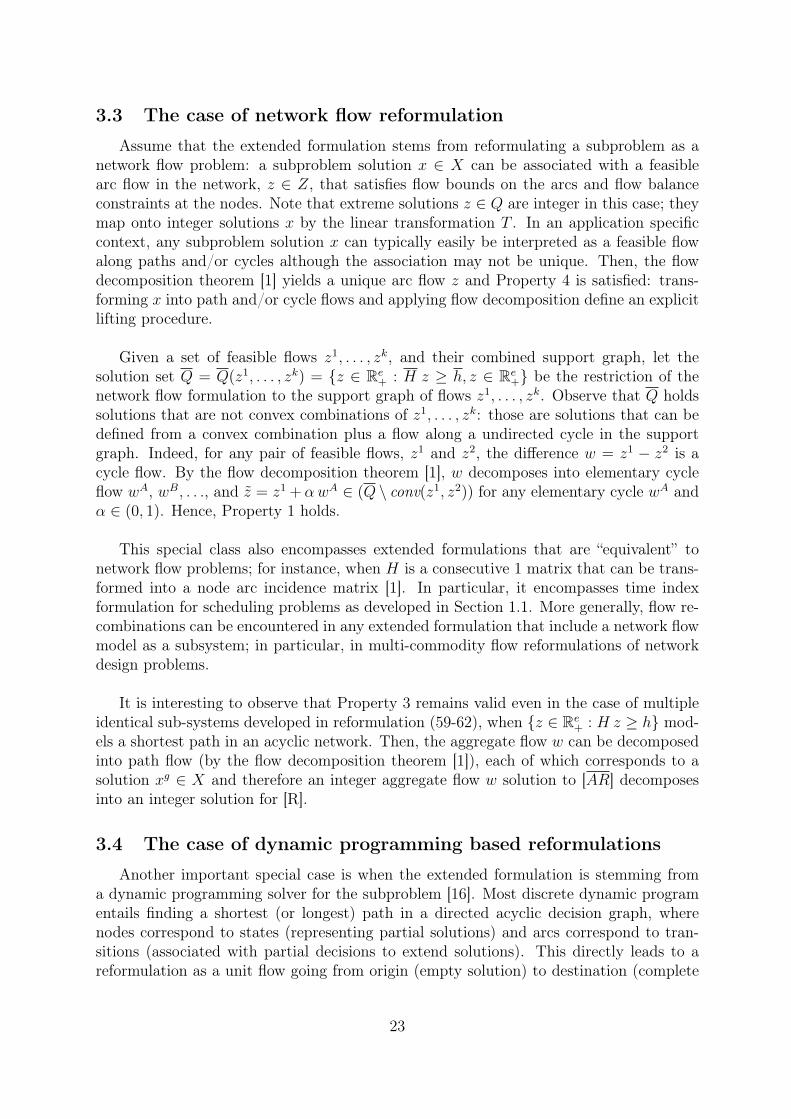
3.3 The case of network flow reformulation

Assume that the extended formulation stems from reformulating a subproblem as anetwork flow problem: a subproblem solution x ∈ X can be associated with a feasiblearc flow in the network, z ∈ Z, that satisfies flow bounds on the arcs and flow balanceconstraints at the nodes. Note that extreme solutions z ∈ Q are integer in this case; theymap onto integer solutions x by the linear transformation T . In an application specificcontext, any subproblem solution x can typically easily be interpreted as a feasible flowalong paths and/or cycles although the association may not be unique. Then, the flowdecomposition theorem [1] yields a unique arc flow z and Property 4 is satisfied: trans-forming x into path and/or cycle flows and applying flow decomposition define an explicitlifting procedure.

Given a set of feasible flows z1, . . . , zk, and their combined support graph, let thesolution set Q = Q(z1, . . . , zk) = {z ∈ Re

+ : H z ≥ h, z ∈ Re+} be the restriction of the

network flow formulation to the support graph of flows z1, . . . , zk. Observe that Q holdssolutions that are not convex combinations of z1, . . . , zk: those are solutions that can bedefined from a convex combination plus a flow along a undirected cycle in the supportgraph. Indeed, for any pair of feasible flows, z1 and z2, the difference w = z1 − z2 is acycle flow. By the flow decomposition theorem [1], w decomposes into elementary cycleflow wA, wB, . . ., and z = z1 +αwA ∈ (Q \ conv(z1, z2)) for any elementary cycle wA andα ∈ (0, 1). Hence, Property 1 holds.

This special class also encompasses extended formulations that are “equivalent” tonetwork flow problems; for instance, when H is a consecutive 1 matrix that can be trans-formed into a node arc incidence matrix [1]. In particular, it encompasses time indexformulation for scheduling problems as developed in Section 1.1. More generally, flow re-combinations can be encountered in any extended formulation that include a network flowmodel as a subsystem; in particular, in multi-commodity flow reformulations of networkdesign problems.

It is interesting to observe that Property 3 remains valid even in the case of multipleidentical sub-systems developed in reformulation (59-62), when {z ∈ Re

+ : H z ≥ h} mod-els a shortest path in an acyclic network. Then, the aggregate flow w can be decomposedinto path flow (by the flow decomposition theorem [1]), each of which corresponds to asolution xg ∈ X and therefore an integer aggregate flow w solution to [AR] decomposesinto an integer solution for [R].

3.4 The case of dynamic programming based reformulations

Another important special case is when the extended formulation is stemming froma dynamic programming solver for the subproblem [16]. Most discrete dynamic programentails finding a shortest (or longest) path in a directed acyclic decision graph, wherenodes correspond to states (representing partial solutions) and arcs correspond to tran-sitions (associated with partial decisions to extend solutions). This directly leads to areformulation as a unit flow going from origin (empty solution) to destination (complete

23

solution). Then, one is again in the special case of Section 3.3.

However, more complex dynamic programs may involve the composition of more thanone intermediate state (representing partial solutions) into a single state (next stage par-tial solution). These can be modeled by hyper-arcs with a single head but multiple tails.Then, the extended paradigm developed by [16] consists in seeing a dynamic program-ming solution as a hyper-path (associated to a unit flow incoming to the final state) in ahyper-graph that satisfy two properties:

(i) acyclic consistency – there exists a topological indexing of the nodes such as, foreach hyper-arc, the index of the head is larger than the index of the tail nodes;

(ii) disjointness – if a hyper-arc has several tails, they must have disjoint predecessorsets.

This characterization avoids introducing an initial state, but instead consider “boundary”arcs that have undefined tails: see Figure 4. The dynamic programs that can be modeledas a shortest path problem are a special case where the hyper-graph only has simple arcswith a single tail and hence the disjointness property does not have to be checked.

Figure 4: Illustration of the recombination of subproblem solutions that are associatedwith hyper-paths in the hyper-graph underlying the paradigm of [16]: nodes are indexedin acyclic order; node 21 represents the final state; hyper-arcs may have multiple tailbut a single head; “boundary” arcs that represent initialization conditions have no tail; asolution is defined by a unit flow reaching the final node 21; when a unit flow exits anhyper-arc, a corresponding unit flow must enter in each of the tail nodes; solutions z1and z2 are depicted on in the hyper-graphs on the left and in the middle; they share acommon intermediate node 19; their recombination, z, is represented in the hyper-graphon the right.

21

7

1

2

3

4

5

6

8

9

10

11

12

13

14

15

16

17

18

19

20

21

7

1

2

3

4

5

6

8

9

10

11

12

13

14

15

16

17

18

19

20

21

7

1

2

3

4

5

6

8

9

10

11

12

13

14

15

16

17

18

19

20

Following [16], consider a directed hyper-graph G = (V ,A), with hyper-arc set A ={(J, l) : J ⊂ V \ {l}, l ∈ V} and associated arc costs c(J, l), a node indexing σ : V →

24

{1, . . . , |V|} such that σ(j) < σ(l) for all j ∈ J and (J, l) ∈ A (such topological indexingexists since the hyper-graph is acyclic). The associated dynamic programming recursiontakes the form:

γ(l) = min(J,l)∈A

{c(J, l) +∑j∈J

γ(j)} .

Values γ(l) can be computed recursively following the order imposed by indices σ, i.e.,for l = σ−1(1), . . . , σ−1(|V|). Solving this dynamic program is equivalent to solving thelinear program:

max{uf : ul −∑j∈J

uj ≤ c(J, l) ∀(J, l) ∈ A} (70)

where f = σ−1(|V|) is the final state node. Its dual is

min{∑

(J,l)∈A

c(J, l) z(J,l) (71)

∑(J,f)∈A

z(J,f) = 1 (72)

∑(J,l)∈A

z(J,l) =∑

(J ′,l′)∈A:l∈J ′

z(J ′,l′) ∀l 6= f (73)

z(J,l) ≥ 0 ∀(J, l) ∈ A} (74)

that defines the reformulation Q for the subproblem.

In this generalized context, [16] gives an explicit procedure to obtain a solution z, defin-ing the hyper-arcs that are in the subproblem solution, from the solution of the dynamicprogramming recursion: the hyper-arc selection is a dual solution to the linear program(70); given the specific assumption on the hyper-graph (acyclic consistency and disjoint-ness), this dual solution z can be obtained through a greedy procedure. So if one uses thedynamic program as oracle, one can recover a solution x and associated complementarysolution z. Alternatively, if subproblem solution x is obtained by another algorithm, onecan easily compute distance labels, ul, associated to nodes of the hyper-graph (ul = thecost of partial solution associated to node l if this partial solution is part of x and ul =∞otherwise) and apply the procedure of [16] to recover the complementary solution z. So,Property 4 is satisfied. The procedure is polynomial in the size of the hyper-graph.

Property 1 also holds. Indeed, given a hyper-path z, let χ(z, J, l) be the characteristicvector of the set of hyper-arcs (J ′, l′) in the hyper-path defined by z. Now consider twohyper-paths z1 and z2 such that z1(J1,l) = 1 and z2(J2,l) = 1 for a given intermediate node l,with J1 6= J2. Then, consider z = z1−χ(z1, J1, l) +χ(z2, J2, l). Note that we have z ∈ Zbut z 6∈ conv(z1, z2), as z1(J1,l) = 1 and z(J1,l) = 0. Such a recombination is illustrated inFigure 4.

3.5 The case of reformulations based on the union of polyhedra

A third important class of reformulations consists of those exploiting one’s ability toformulate the union of polyhedra. Assume Qk = {z ∈ Re

+ : Hkz ≤ hk} is an extended

25

Figure 5: The union of three polyhedra

formulation for Xk and X = ∪kXk while Ck := {z ∈ Re+ : Hkz ≤ 0} = C ∀k, then

Q = {(z, δ) ∈ Re+ × [0, 1]K : z =

∑k

zk;∑k

δk = 1;Hkzk ≤ hk δk∀k}

defines an extended formulation for X. Figure 5 illustrates three polyhedron and theirconvex combination defined by Q.

Let us consider how does Property 1 applies in such case. For a given z ∈ Z, thereexists an associated δk = 1 such that z = zk. Then, in [RLP ] restricted to z, any LP solu-tion to Qk

(zk) (defined as the restriction of Qk to zk) is feasible and not just zk. However,even after adding several subproblem solutions for each subsystem Qk, recombinationshall remain internal to each subsystem Q

k, i.e., at any stage, the restricted master [RLP ]do not allow combinations of the solutions associated to different subsystems k other thantheir convex combination. In other words, recombinations only arise within each of thesubsystem Q

k and not between them. The example of Section 1.3 is an application basedon such union of polyhedra.

4. Numerical experimentationConsider the three formulations introduced in Section 2: the compact formulation [F],

the extended formulation [R], and the standard Dantzig-Wolfe reformulation [M], withtheir respective LP relaxation [FLP ], [RLP ], and [MLP ]. Here, we report on comparativenumerical experiments with column(-and-row) generation for [RLP ] and [MLP ], and a di-rect LP-solver approach applied to [RLP ] (or [FLP ], when the direct approach to [RLP ] isimpractical). The column(-and-row) generation algorithm has been implemented gener-ically within the software platform BaPCod [27] (a problem-specific implementation islikely to produce better results). The master program is initialized with either a singleartificial variable, or one for each linking constraint, or a heuristic solution. For column-and-row generation, all extended formulation variables z that form the pricing subproblemsolution are added to the restricted master, whether or not they have negative reducedcost. CPLEX 12.1 was used to attempt to solve directly [RLP ] or [FLP ]. CPLEX 12.3is used to solve the restricted master linear programs, while the MIP subproblems aresolved using a specific oracle.

26

For applications where the subproblem is a knapsack problem, we used the solver ofPisinger [19]. Then, when using column-and-row generation, the solution in the originalx variables is “lifted” to recover an associated solution z using a simple combinatorialprocedure. For a 0-1 knapsack, we sort the items i for which x∗i = 1 in non-increasingorder of their size, si, and let z∗uv = 1 for the arc (u, v) such that u =

∑j<i sjx

∗j and

v =∑

j≤i sjx∗j . Note that this specific lifting procedure selects one representative amongs

all equivalent solutions in the arc-space, automatically eliminating some symmetries. Itcan be extended to integer knapsack problems. For the other applications consideredhere, the subproblems are solved by dynamic programming and hence the z∗ solution isobtained directly: z∗uv = 1 if the optimum label at v is obtained using state transitionfrom u.

Results of Tables 2 to 7, are averages over randomly generated instances. The columnheaded by “cpu” reports the average computational time (in seconds on a Dell PowerEdge1950 workstation with 32 Go of Ram or an Intel Xeon X5460 3.16 GHz processor); “it”denotes the average number of iterations in the column(-and-row) generation procedure(it represents the number of calls to the restricted master solver); “v(F1

F2)” (resp. “c(F1

F2)”)

denote the average number of variables (resp. constraints) generated for formulation F1

expressed as a percentage of the number of variables (resp. constraints) generated forF2. Additionally, “%gap” (reported in some applications) denotes the average differencebetween dual bound and best primal bound known (the optimum solution in most cases),as a percentage of the latter. Bounds are rounded to the next integer for integer objectives.

To validate the stabilization effect of the column-and-row generation approach, weshow how it compares to applying stabilization in a standard column generation ap-proach. We point out that stabilization by recombination is of a different nature thanstandard stabilization techniques. To illustrate this, we show that applying both standardstabilization and column recombination together leads to a cumulative effect. For theseexperiments, the “standard stabilization technique” that we use is a dual price smoothingtechnique originally proposed by Wentges [30]. It is both simple and among the mosteffective stabilization techniques. It consists in solving the pricing subproblem for a linearcombination, π, of the current restricted master dual solution, π, and the dual solutionwhich gave the best Lagrangian bound, π: i.e., π = απ+(1−α)π, where α ∈ [0, 1). Thus,α = 0 means that no stabilization by smoothing is used.

4.1 Parallel Machines Scheduling

For the machine scheduling problem of Section 1.1, our objective function is the totalweighted tardiness (this problem is denoted as P ||

∑wjTj). Instance size is determined

by a triple (n,m, pmax), where n is the number of jobs, m is the number of machines, andpmax is the maximum processing time of jobs. Instances are generated using the procedureof [21]: integer processing times pj are uniformly distributed in interval [1, 100] and integerweights wj in [1, 10] for jobs j, j = 1, . . . , n, while integer due dates have been generatedfrom a uniform distribution in [P (1−TF −RDD/2)/m, P (1−TF +RDD/2)/m], whereP =

∑j pj, TF is a tardiness factor, and RDD is a relative range of due dates, with

TF,RDD ∈ {0.2, 0.4, 0.6, 0.8, 1}. For each instance size, 25 instances were generated, one

27

for each pair of parameters (TF,RDD).

Cplex Col. gen. Col-&-row Hyb. col-&-row and relativefor [RLP ] for [MLP ] g. for [RLP ] g. for [RLP ] size

m n pmax cpu it cpu it cpu it cpu v(RR) v(MR

) c(MR

)1 25 50 1.6 331 0.5 50 0.3 106 0.3 5.3 45.6 4.11 50 50 18.8 1386 19.7 76 2.9 207 2.8 3.2 72.7 3.71 100 50 304.2 8167 1449.5 104 24.8 354 19.4 2.3 138.0 4.01 25 100 7.1 337 0.9 72 0.9 124 0.8 3.8 33.8 2.01 50 100 132.6 1274 24.2 107 8.9 246 8.6 2.7 43.1 1.81 100 100 2332.0 8907 1764.4 144 90.3 455 61.3 1.9 103.2 1.92 25 100 4.1 207 0.3 63 0.2 97 0.2 3.9 40.0 3.92 50 100 109.2 645 5.7 94 1.7 173 1.9 2.8 39.9 3.52 100 100 3564.4 2678 115.5 117 14.3 319 14.9 2.1 59.3 3.74 50 100 18.7 433 1.5 90 0.6 167 0.7 3.0 45.0 6.64 100 100 485.7 1347 27.9 113 4.7 295 5.2 2.2 56.2 7.24 200 100 >2h 4315 409.7 148 36.1 561 39.7 1.5 69.7 7.6

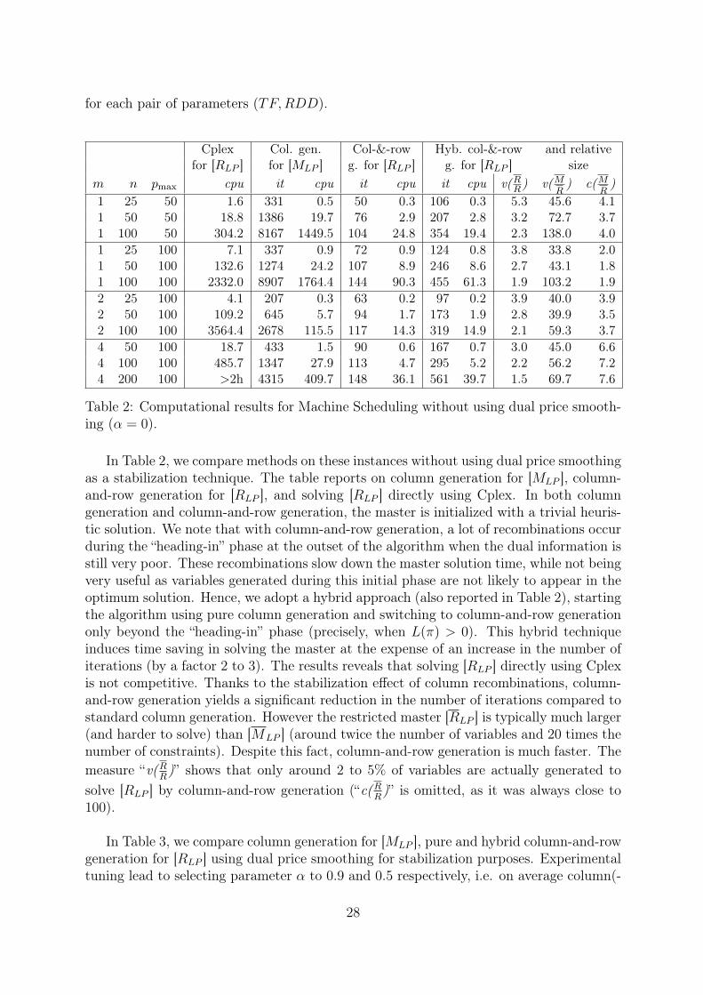
Table 2: Computational results for Machine Scheduling without using dual price smooth-ing (α = 0).

In Table 2, we compare methods on these instances without using dual price smoothingas a stabilization technique. The table reports on column generation for [MLP ], column-and-row generation for [RLP ], and solving [RLP ] directly using Cplex. In both columngeneration and column-and-row generation, the master is initialized with a trivial heuris-tic solution. We note that with column-and-row generation, a lot of recombinations occurduring the “heading-in” phase at the outset of the algorithm when the dual information isstill very poor. These recombinations slow down the master solution time, while not beingvery useful as variables generated during this initial phase are not likely to appear in theoptimum solution. Hence, we adopt a hybrid approach (also reported in Table 2), startingthe algorithm using pure column generation and switching to column-and-row generationonly beyond the “heading-in” phase (precisely, when L(π) > 0). This hybrid techniqueinduces time saving in solving the master at the expense of an increase in the number ofiterations (by a factor 2 to 3). The results reveals that solving [RLP ] directly using Cplexis not competitive. Thanks to the stabilization effect of column recombinations, column-and-row generation yields a significant reduction in the number of iterations compared tostandard column generation. However the restricted master [RLP ] is typically much larger(and harder to solve) than [MLP ] (around twice the number of variables and 20 times thenumber of constraints). Despite this fact, column-and-row generation is much faster. Themeasure “v(R

R)” shows that only around 2 to 5% of variables are actually generated to

solve [RLP ] by column-and-row generation (“c(RR)” is omitted, as it was always close to

100).

In Table 3, we compare column generation for [MLP ], pure and hybrid column-and-rowgeneration for [RLP ] using dual price smoothing for stabilization purposes. Experimentaltuning lead to selecting parameter α to 0.9 and 0.5 respectively, i.e. on average column(-

28

Col. gen. Col-&-row Hyb. col-&-row and relativefor [MLP ], g. for [RLP ], for [RLP ], α = 0.5 sizeα = 0.9 α = 0.5

m n pmax it cpu it cpu it cpu v(RR) v(M

R) c(M

R)

1 25 50 145 0.2 45 0.2 84 0.2 4.1 31.5 4.31 50 50 341 2.5 70 2.3 154 1.8 2.5 36.9 3.81 100 50 746 26.1 91 22.0 266 12.6 1.8 30.8 4.01 25 100 150 0.2 61 0.5 96 0.4 2.6 26.6 2.21 50 100 354 3.8 91 6.8 172 4.0 1.7 25.7 1.91 100 100 781 39.5 115 78.6 299 31.1 1.3 28.8 1.92 25 100 142 0.2 55 0.2 87 0.2 3.3 37.5 4.12 50 100 323 1.7 84 1.5 158 1.6 2.2 32.2 3.62 100 100 715 17.3 102 12.4 275 11.3 1.6 29.2 3.74 50 100 287 0.6 83 0.5 154 0.6 2.6 39.5 6.74 100 100 638 8.7 102 4.1 264 4.6 1.8 38.7 7.24 200 100 1553 87.7 136 33.5 481 33.4 1.2 36.3 7.6

Table 3: Computational results for Machine Scheduling using dual price smoothing as astabilization technique.

and-row) generation takes the least time to execute when α is fixed to these values. Therestricted masters are initialized by a single artificial column, except in pure column-and-row generation, in which the master is initialized with a trivial heuristic solution.Here again, the hybrid approach consists in using standard column generation during the“heading-in” phase and switching to column-and-row generation when L(π) > 0. Resultsof Table 3 show that smoothing yields a speed-up in both standard column generationand column-and-row generation, but it is less impressive for the latter as the methodwas already stabilized by the recombination effect. The difference in cpu time betweenthe two methods increases when either processing times are smaller (allowing for morerecombinations) and when number of machines and jobs are larger.

In Table 4, we compare the column(-and-row) generation approaches on the arc-indexed formulation proposed by Pessoa et al. [18] where a binary variable zijt is definedfor every pair of jobs (i, j) and every period t: zijt = 1 if job i finishes and job j startsin period t. Then, flow conservation constraints are defined for every couple (j, t). Goingto this larger extended space has some advantages: (i) direct repetitions of jobs are for-bidden by not defining variable ziit; and (ii) a simple dominance rule is incorporated bynot defining variable zijt if permuting jobs i and j decreases the total cost. The resultingstrengthening of the LP relaxation bound is, in our experiments, on average 0.38% forsingle-machine instances, 0.28% for two-machine instances, and 0.13% for four-machineinstances. This difference is significant given the fact that the time-indexed formulationis already very strong. However, the arc-indexed formulation has huge size (solving [RLP ]directly is excluded). Moreover, the complexity of the dynamic program for solving thepricing problem increases to O(n2T ) and hence time for pricing dominates the overall cputime. In this context, reducing the number of iterations is key, which gives the advantageof the column-and-row generation approach. For this reason, we did not use the hybrid

29

column-and-row generation approach here. For the results of Table 4, experimental tuninglead to selecting smoothing parameter α to 0.9 and 0.7 respectively, while the restrictedmaster is initialized by a single artificial column for standard column generation and us-ing a trivial heuristic solution for column-and-row generation. Using a column-and-rowgeneration approach yields a reduction of both iterations and cpu time by factor up to5.6. The number of variables and constraints in the final restricted master [RLP ] is onlya very small fraction of that of [RLP ].

Col. gen. Col-&-row g. and relativefor [Marc

LP ], α = 0.9 for [RarcLP ], α = 0.7 size

m n pmax it cpu it cpu v(RR) c(R

R) v(M

R) c(M

R)

1 25 50 127 0.5 85 0.5 0.30 1.3 23.1 11.01 50 50 332 11.7 117 5.6 0.09 0.8 23.7 9.51 100 50 734 198.1 161 57.3 0.03 0.4 21.8 9.51 25 100 128 1.1 100 1.2 0.13 0.6 24.5 12.91 50 100 328 25.7 160 16.0 0.05 0.4 21.5 9.71 100 100 758 466.3 197 144.7 0.02 0.3 19.9 8.32 25 100 145 0.7 89 0.5 0.16 1.1 42.6 12.02 50 100 332 13.0 140 5.9 0.07 0.7 32.6 11.32 100 100 730 203.7 186 54.4 0.02 0.4 27.1 10.54 50 100 286 5.6 145 3.1 0.08 1.1 42.6 13.24 100 100 618 83.5 197 27.5 0.03 0.6 33.6 13.34 200 100 1530 2233.2 275 389.9 0.01 0.2 30.4 12.0

Table 4: Computational results for Machine Scheduling using smoothing and an arc-indexed formulation.

4.2 Bin Packing

For the bin packing problem of Section 1.2, we compared solving [FLP ] using Cplex(as solving [RLP ] directly is impractical), standard column generation for [MLP ], and purecolumn-and-row generation for [RLP ]. Instance classes “a2”, “a3”, and “a4” (the numberrefers to the average number of items per bin) contain instances with bin capacity equal to4000 where item sizes are generated randomly in intervals [1000, 3000], [1000, 1500], and[800, 1300], respectively. Results in Table 5 are averages over 5 instances. Experimentaltuning lead to selecting smoothing parameter α to 0.85 for both approaches, while therestricted master is initialized with a trivial heuristic solution. Here, “gap” denotes theabsolute value of the difference between dual bound and the optimum solution (which wecomputed by branch-and-price); it is always zero for formulations [MLP ] and [RLP ]. Thepercentage gap is also given under “%gap”. Although the reformulation is based on As-sumption 2, the dual bound obtained solving [RLP ] is the same as for [MLP ] on the testedinstances. The column-and-row generation for [RLP ] outperforms column generation for[MLP ] only when the number of items per bin increases (i.e., for class “a4”), as other-wise the potential for column recombination is very limited. The number of iterations isreduced when using column-and-row, but this might not compensate for the extra timerequired to solve the master, as here pricing required only between 4% and 30% of the

30

overal cpu time. The average relative size (v(MR), c(M

R)) in percent is respectively (82, 36)

for class “a2”, (39, 37) for class “a3”, and (52, 32) for class “a4”; while the percentage (v(RR),

c(RR)) reported in Table 5 are very small.

Cplex Col. gen. Col-&-row g.for [FLP ] for [MLP ], α = 0.85 for [RLP ], α = 0.85

class n gap %gap cpu it cpu it cpu v(RR) c(R

R)

“a2” 200 5.6 5.2 0.1 439 0.3 281 0.5 0.21 14.9400 8.6 4.0 0.8 1001 1.2 599 2.0 0.15 25.7800 6.6 1.6 10.4 2725 6.8 1331 12.2 0.13 40.8

“a3” 200 4.0 6.0 0.1 158 0.2 124 0.2 0.16 15.1400 8.6 6.4 0.6 298 0.7 192 0.8 0.10 24.7800 17.4 6.5 7.7 596 5.5 297 4.8 0.08 38.7

“a4” 200 0.8 1.5 0.1 400 0.8 253 1.0 0.27 18.9400 1.8 1.7 0.6 841 5.4 414 4.5 0.17 29.0800 2.8 1.3 5.8 1662 38.6 602 16.3 0.13 41.6

Table 5: Computational results for Bin Packing using dual price smoothing as a stabi-lization technique.

4.3 Generalized assignment problem

In the Generalized Assignment Problem (GAP), the objective is to find a maximumprofit assignment of a set J = {1, . . . , n} of jobs to a set I = {1, . . . ,m} of machines suchthat each job is assigned to precisely one machine subject to capacity restrictions on themachines. A compact formulation in terms of binary variables xij that indicate whetherjob j is assigned to machine i, is:

[F] ≡ min{∑i,j

cijxij :∑i

xij = 1 ∀j,∑j

aijxij ≤ bi ∀i, xij ∈ {0, 1} ∀i, j}, (75)

where cij ∈ N is the cost of assigning job j to machine i, aij ∈ N is job j’s claim on thecapacity of machine i, and bi ∈ N is the capacity of machine i. The binary knapsacksubproblem consists in selecting a job assignment for a single machine i: X i = {xi ∈{0, 1}n :

∑j aijxij ≤ bi

}. It can be reformulated as a shortest path problem:

Zi ={zi ∈ {0, 1}bi×n :

n∑j=0

zij0 = 1,n∑j=0

(zijt − zi,j,t−aij) = 0 ∀t ∈ {1, . . . , bi − 1}}

(76)

where binary variable zijt indicates whether job j uses capacity interval [t, t + aij) onmachine i.

In Table 6, we compare three approaches: solving [FLP ] using Cplex (as solving [RLP ]directly is impractical); solving [MLP ] by standard column generation; and solving [RLP ]

31

by pure column-and-row generation. The three approaches were tested on instances fromthe OR-Library with 100, 200 and 400 jobs, and 5, 10, 20 and 40 machines. The in-stances in classes C, D, and E were used, since the instances in classes A and B are easyfor modern MIP solvers. Results are averages over 3 instances, one for each class. Forcolumn(-and-row) generation, experimental tuning lead to selecting smoothing parameterα to 0.85 and 0.5 respectively, while the restricted master is initialized respectively witha single artificial column and a trivial heuristic solution. Column-and-row generation ismuch faster than standard column generation, but it produces dual bounds that are muchworse (almost as bad as those obtained solving [FLP ]). This is explained by the fact thatthe reformulation is done under Assumption 2, relaxing the subproblem to an unboundedknapsack problem (76).

Cplex Col. gen. Col-&-row g. and relativefor [FLP ] for [MLP ], α = 0.85 for [RLP ], α = 0.5 size

m n %gap cpu it %gap cpu it %gap cpu v(RR) v(M

R) c(M

R)

20 100 1.17 0.05 201 0.09 1.4 31 0.40 1.3 2.1 116.2 8.510 100 0.55 0.03 229 0.10 1.2 33 0.35 1.1 1.9 83.2 9.05 100 0.26 0.01 295 0.05 2.2 35 0.20 1.1 1.6 61.8 9.020 200 0.28 0.10 358 0.02 11.9 37 0.17 8.1 1.2 109.1 8.410 200 0.17 0.05 448 0.04 24.6 38 0.14 7.7 1.0 78.7 8.55 200 0.07 0.02 637 0.02 70.5 34 0.07 6.8 0.9 62.1 8.440 400 0.15 0.51 591 0.03 131.1 41 0.11 80.9 0.8 146.9 8.020 400 0.09 0.23 696 0.03 407.1 41 0.08 65.9 0.6 102.9 8.110 400 0.04 0.11 909 0.01 1338.8 41 0.04 58.8 0.5 75.0 8.1

Table 6: Computational results for Generalized Assignment using dual price smoothingas a stabilization technique.

We have also experimented with applying the column-and-row generation approachto a larger extended formulation obtained directly from the dynamic programming solverfor the pricing sub-problem as explained in Section 3.4. As this larger formulation modelsa bounded knapsack subproblem, the LP bound then coincides with the one given bythe standard column generation. In our experiments, column-and-row generation leadto a reduction of iterations by a factor 3 on average. However, the restricted masterof the column-and-row generation approach is much larger than with standard columngeneration. Hence, this approach is not competitive in terms of cpu time.

4.4 Multi-Item Multi-Echelon Lot-Sizing

The Multi-Item Lot-Sizing problem consists in planning production so as to satisfydemands dkt for item k = 1, . . . , K over a discrete time horizon with period t = 1, . . . , Teither from stock or from production. The production of an item entails production stages(echelons) e = 1, . . . , E, each of which takes place on a different machine that can onlyprocess one product in each period (under the so-called small bucket assumption). A

32

compact formulation is:

[F] ≡ min∑ket

(cket xket + fket y

ket) (77)∑

k

yket ≤ 1 ∀e, t (78)

t∑τ=1

xkeτ ≥t∑

τ=1

xke+1,τ ∀k, e < E, t (79)

t∑τ=1

xkEτ ≥ Dk1t ∀k, t (80)

xket ≤ DktT y

ket ∀k, e, t (81)

xket ≥ 0 ∀k, e, t (82)yket ∈ {0, 1} ∀k, e, t , (83)

where variables xket are the production of item k at echelon e in period t (at unit costcket) and yket take value 1 if the production of item k at echelon e is setup in periodt (at a fixed cost fket); Dk

1t =∑t

τ=1 dkτ . The stock values can be computed as sket =∑t

τ=1 xkeτ −

∑tτ=1 x

ke+1,τ ; their costs have been eliminated (they are included in cket).

For the single item problem, there exists an optimal solution where at each echelonand period either there is an incoming stock or an incoming production but not both, i.e.,such that xket sket = 0 ∀e, t. Hence, production can be restricted to lots corresponding toan interval of demands. This dominance property can be exploited to solve single itemsubproblems by dynamic programming in polynomial time [20]. A backward dynamicprogram (DP) can be defined where the states are associated with quadruples (e, t, a, b)denoting the fact of having at echelon e in period t accumulated a production that iscovering exactly the demand Dk

ab for the final product of item k. It is defined for t ≤ a ≤b ≤ T and e = 1, . . . , E. The backward recursion is:

V (e, t, a, b) = min{V (e, t+1, a, b), minl=a,...,b

{V (e+1, t, a, l)+cketDkal+f

ket+V (e, t+1, l+1, b)}}

for all e = E, . . . , 1, t = T, . . . , 1, a = T, . . . , 1, and b = T, . . . , a. By conventionV (e, t, a, b) = 0 if a > b. The initialization is V (E + 1, t, a, b) = 0. The optimum isgiven by V ∗ = V (1, 1, 1, T ).

From this dynamic program, one can reformulate the single item subproblem as select-ing a decision tree in an hyper-graph whose nodes are the states of the above DP. The DPtransition can be associated to flow on hyper-arcs: zke,t,a,l,b = 1 if at echelon e ∈ {1, . . . , E}in period t ∈ {1, . . . , T} the production of item k is made to cover demands from perioda ∈ {t, . . . , T} to period l ∈ {a − 1, . . . , T}, while the rest of demand interval, i.e. de-mands from period l+ 1 to period b ∈ {l, . . . , T}, will be covered by production in futureperiods. If l = a− 1, there is no production; this can only happen when a > t. While ifl = b, the whole demand interval, Dk

ab, is produced in t. The associated cost, cke,t,a,l,b, is(cketD

kal + fket) if l ≥ a and zero if l = a− 1. For the initial echelon e = 1, variables zk1,t,a,l,b

33

are only defined for b = T . For the first period t = 1, they are only defined for a = t = 1.This leads to reformulation:

[R] ≡ min∑

e,t,a,l,b,k

cke,t,a,l,b zke,t,a,l,b (84)

E∑e=1

∑a,l,b,k:l≥a,Dk

al>0

zke,t,a,l,b ≤ 1 ∀e, t (85)

∑l

zk1,1,1,l,T = 1 ∀k (86)∑l

zke,t,a,l,b −∑τ≤a

zke,t−1,τ,a−1,b −∑τ≥b

zke−1,t,a,b,τ = 0 ∀k, e, t, a, b (87)

zke,t,a,l,b ∈ {0, 1} ∀k, e, t, a, l, b , (88)

which results from subproblem reformulation Zk defined by constraints (86-88) for a fixedk. Note that constraints (87) are only defined for t > 1 and b = T when e = 1; while,when e > 1, they are only defined for a = t when t = 1.

In Table 7, we compare standard column generation and pure column-and-row gener-ation respectively for [MLP ] and [RLP ]. (Solving formulation [RLP ] directly with Cplexis impractical.) Experimental tuning lead to selecting smoothing parameter α to 0.85and 0.4 respectively, while the restricted master is initialized with a trivial heuristic so-lution. Results are averages over 5 instances generated randomly, with a number of jobsK ∈ {10, 20, 40}, a number of periods T ∈ {50, 100, 200, 400}, while setup costs are uni-formly distributed in [20, 100], production costs are zero, and storage cost hke are generatedas hke−1 + γ, where γ is uniformly distributed in interval [1, 5]. For each period, there is apositive demand for 3 items on average. Demands are generated using a uniform distri-bution on interval [10, 20].

For the column generation approach to [MLP ], instances get easier as the number ofitems increases. Indeed, instances with more items have fewer feasible solutions given thesingle mode constraints. The column-and-row generation clearly outperforms standardcolumn generation on all instances except those with 2 echelons and 50 periods. Thenumber of iterations for column-and-row generation is up to an order of magnitude smaller.This shows the benefit of recombinations of decision trees (as illustrated in Figure 4) thattake place in this application. This benefit increases with the number of echelons and theratio T

K. Once again, the percentages (v(R

R), c(R

R)) are very small. These experiments

shows that very large extended formulations can be tractable when solved by column-and-row generation.

ConclusionThe “column-and-row generation” has been presented here as a generalization of stan-

dard column generation, in the spirit of [28]. Our aim was to explain exactly when itshould be considered, how it works, why it can be comparatively more efficient, and what

34

Col. gen. Col-&-row g. and relativefor [MLP ], α = 0.85 for [RLP ], α = 0.4 size

K T it cpu it cpu v(RR) c(R

R) v(M

R) c(M

R)

2 echelons10 50 126 1.7 29 1.6 0.57 1.32 26.4 3.420 50 79 1.8 27 3.1 0.44 1.06 17.2 2.110 100 332 38.0 43 8.1 0.15 0.36 34.2 3.220 100 232 31.5 38 20.0 0.14 0.34 21.7 1.7

3 echelons10 50 187 11.8 38 5.5 0.16 1.08 24.3 3.220 50 112 12.0 33 9.8 0.12 0.82 16.9 2.110 100 509 454.5 49 36.4 0.02 0.27 33.5 3.320 100 362 520.4 48 103.1 0.02 0.27 21.4 1.6

5 echelons10 50 296 62.6 48 16.3 0.10 0.91 24.4 3.320 50 223 66.8 42 34.3 0.07 0.69 18.8 2.210 100 882 4855.9 61 134.0 0.01 0.24 32.9 3.220 100 750 4657.8 56 386.1 0.01 0.22 22.3 1.7

Table 7: Computational results for multi-echelon multi-item lot-sizing

are its practical performance on a scope of applications. Our generic presentation madeit straightforward to extend the method to the case where the Dantzig-Wolfe decompo-sition paradigm is based on a subproblem approximate extended formulation. Then, bypricing on the subproblem integer hull, one can derive Lagrangian dual bounds that serveto define early termination of the algorithm before meeting the reduced cost conditions.We emphasized that the algorithm aims at identifying optimal dual prices (Lagrangianmultipliers) for the linking constraints, disregarding the dual value of the other constraintsof the extended formulation.

In the literature, a motivation for working with an extended formulation and usingthe “column-and-row generation” methodology has been the use of the richer variablespace of the extended formulation to define cuts or branching constraints. This benefitcan be achieved by working with a pricing subproblem in the extended variable space,while working with the traditional master program and a standard column generationapproach. Here, we highlighted the benefit of working with a master program expressedin the variable space of the extended formulation, while possibly working with a subprob-lem compact formulation and implementing a lifting of the subproblem solutions. Theinterest is to achieve faster convergence thanks to recombinations of previously gener-ated subproblem solutions into new points that are not in the convex hull of currentlygenerated subproblem solutions. By working in the variable space of the extended formu-lation in both master and subproblem, one can combine the two above benefits to developbranch-and-price-and-cut based on column-and-row generation (such application specificalgorithm is beyond the scope of this paper).

We considered two generic situations where the recombination property (Property 1)

35

holds: when the reformulation stems from a network flow model, or a dynamic program-ming subproblem solver. More generally, this analysis could be extended to generalizedflow reformulations, or to reformulations based on a branched polyhedral system [13].Other examples where the recombination property holds include special cases such asthe example of Section 1.3, where subproblem solutions that differ only by the value ofthe continuous variables are all implicitly defined in the restricted reformulation. This islinked to the concept of “base-generators”, as developed in [28], that are extracted fromregular columns by keeping only the fixed values of the “important” variables in the sub-problem solution.

The recombination property leading to a reduction in the number of iterations canbe understood as a stabilization technique for column generation. “Disaggregation” helpsconvergence as it is numerically demonstrated in many studies related to column genera-tion. For instance, in the presence of block diagonal systems, good practice is to defineseparate columns for each block, or even to artificially differentiate commodities to createblock diagonality as illustrated for origin-destination flow problems in [12]; another ex-ample is the disaggregation of the time horizon used by [3] for a scheduling application.In the example of Section 1.3, the disaggregation amounts to defining “base-generators”associated to the integer part of the subproblem solution.

The recombination property is closely related to the concept of “exchange vectors” instandard column generation approach [28]; the latter are columns defining rays in thelattice of subproblem solutions (for instance the elementary cycles of Section 3.3 definerays). Using a convex combination of regular columns and exchange vectors allows oneto define new solutions that are outside the convex hull of already generated subproblemsolutions. Exchange vectors define so-called dual cuts (valid inequalities for dual prices)in the dual master program [22].

When the subproblem reformulation is not actually an exact extended formulation forit (i.e., under Assumption 2), there are typically even more recombinations in the relaxedsubproblem solution space. The relaxation can imply a weakening of the dual bound, asillustrated on the generalized assignment application, or no difference in dual bound as inthe bin packing case. Relaxing Assumption 1 into Assumption 2 is related to the conceptof the “state space relaxation” for column generation as presented in [28]. It can also beinterpreted as the development of a column-and-row generation approach based on anapproximated extended formulation for the subproblem as underlined by the proposal ofVan Vyve and Wolsey [26].

Our numerical comparative study of column-and-row generation illustrates the experi-mental trade-off between the comparative acceleration of convergence, the potential lossesof quality in dual bounds (under Assumption 2), and the higher computing time requiredto solve the restricted master (due to its larger size and potential symmetries). Therecommendation that arises from our numerical experiments is to adopt column-and-rowgeneration instead of a standard column generation approach when (i) the subproblemsolution space offers many possible column recombinations; (ii) the extended formulationoffers a strong enough relaxation of the pricing problem (when working under Assump-

36

tion 2); and (iii) the pricing procedure dominates the cpu consumption (so that theincrease in master solution time is marginalized). We have shown that column-and-rowgeneration makes it tractable to consider much stronger/larger extended formulations,with more combinatorial structure built into the pricing subproblem, while generatingonly a very small percentage of its variables and constraints.

AcknowledgmentsWe thank J. Desrosiers, E. Uchoa, and L. A. Wolsey for constructive exchanges on

this paper and their suggestions for improvements.

References[1] R. K. Ahuja, T. L. Magnanti, and J. B. Orlin. Network Flows: Theory, Algorithms

and Applications. Prentice Hall, Englewood Cliffs, New Jersey, 1993.

[2] J. F. Benders. Partitioning procedures for solving mixed-variables programmingproblems. Numerische Mathematik, 4:238–252, 1962.

[3] L.-Ph Bigras, M. Gamache, and G. Savard. Time-Indexed Formulations and theTotal Weighted Tardiness Problem. INFORMS Journal on Computing, 20(1):133–142, 2008.

[4] V. Chvátal. Linear programming. Freeman, 1983.

[5] K.L. Croxton, B. Gendron, and T.L. Magnanti. Variable disaggregation in networkflow problems with piecewise linear costs. Operations Research, 55:146–157, 2007.

[6] G. Desaulniers. Branch-and-price-and-cut for the split-delivery vehicle routing prob-lem with time windows. Operations Research, 58(1):179–192, 2010.

[7] D. Feillet, P. Dejax, M. Gendreau, and C. Gueguen. Vehicle routing with timewindows and split deliveries. Technical Paper 2006-851, Laboratoire d’Informatiqued’Avignon, 2006.

[8] D. Feillet, M. Gendreau, A. L. Medaglia, and J. L. Walteros. A note on branch-and-cut-and-price. Operations Research Letters, 38(5):346 – 353, 2010.

[9] M. Fischetti and D. Vigo. A branch-and-cut algorithm for the resource-constrainedarborescence problem. Networks, 29:55–67, 1996.

[10] A. Frangioni and B. Gendron. 0-1 reformulations of the multicommodity capacitatednetwork design problem. Discrete Applied Mathematics, 157(6):1229 – 1241, 2009.

[11] A. Frangioni and B. Gendron. A stabilized structured Dantzig-Wolfe decompositionmethod. Research report CIRRELT-2010-02, Interuniversity Research Centre onEnterprise Networks, Logistics and Transportation, 2010.

37

[12] K. L. Jones, I. J. Lustig, J. M. Farvolden, andW. B. Powell. Multicommodity networkflows: The impact of formulation on decomposition. Mathematical Programming,62:95–117, 1993.

[13] V. Kaibel and A. Loos. Branched polyhedral systems. In Friedrich Eisenbrandand F. Shepherd, editors, Integer Programming and Combinatorial Optimization,volume 6080 of Lecture Notes in Computer Science, pages 177–190. Springer Berlin/ Heidelberg, 2010.

[14] A. Löbel. Vehicle scheduling in public transit and lagrangean pricing. ManagementScience, 44(12):1637–1649, 1998.

[15] J. W. Mamer and R. D. McBride. A decomposition-based pricing procedure for large-scale linear programs: An application to the linear multicommodity flow problem.Management Science, 46(5):693–709, 2000.

[16] R. K. Martin, R. L. Rardin, and B. A. Campbell. Polyhedral Characterization ofDiscrete Dynamic Programming. Operations Research, 38(1):127–138, 1990.

[17] I. Muter, I. Birbil, and K. Bülbül. Simultaneous column-and-row generation forlarge-scale linear programs with column-dependent-rows. http://www.optimization-online.org/DB_FILE/2010/11/2815.pdf, 2010.

[18] A. Pessoa, E. Uchoa, M. Poggi de Aragão, and R. Rodrigues. Exact algorithm over anarc-time-indexed formulation for parallel machine scheduling problems. MathematicalProgramming Computation, 2:259–290, 2010.

[19] D. Pisinger. A minimal algorithm for the 0-1 knapsack problem. Operations Research,45:758–767, 1997.

[20] Y. Pochet and L. A. Wolsey. Production planning by mixed integer programming.Springer, 2006.

[21] C. N. Potts and L. N. Van Wassenhove. A Branch and Bound Algorithm for theTotal Weighted Tardiness Problem. Operations Research, 33(2):363–377, 1985.

[22] J. M. Valério de Carvalho. Using Extra Dual Cuts to Accelerate Column Generation.INFORMS Journal on Computing, 17(2):175–182, 2005.

[23] J.M. Valério de Carvalho. Exact solution of bin packing problems using columngeneration and branch and bound. Annals of Operations Research, 86:629–659, 1999.

[24] J. M. van den Akker, J. A. Hoogeveen, and S. L. van de Velde. Parallel machinescheduling by column generation. Operations Research, 47(6):862–872, 1999.

[25] J.M. van den Akker, C.A.J. Hurkens, and M.W.P. Savelsbergh. Time-Indexed Formu-lations for Machine Scheduling Problems: Column Generation. INFORMS Journalon Computing, 12(2):111–124, 2000.

[26] M. Van Vyve and L. A. Wolsey. Approximate extended formulations. MathematicalProgramming, 105:501–522, 2006.

38

[27] F. Vanderbeck. Bapcod – a branch-and-price generic code. University of Bordeaux,INRIA Research team ReAlOpt.

[28] F. Vanderbeck and M. W. P. Savelsbergh. A generic view of Dantzig-Wolfe decom-position in mixed integer programming. Operations Research Letters, 34(3):296–306,2006.

[29] F. Vanderbeck and L. A. Wolsey. Reformulation and decomposition of integer pro-grams. In Michael Jünger, Thomas M. Liebling, Denis Naddef, George L. Nemhauser,William R. Pulleyblank, Gerhard Reinelt, Giovanni Rinaldi, and Laurence A. Wolsey,editors, 50 Years of Integer Programming 1958-2008, pages 431–502. Springer BerlinHeidelberg, 2010.

[30] P. Wentges. Weighted Dantzig–Wolfe decomposition for linear mixed-integer pro-gramming. International Transactions in Operational Research, 4(2):151–162, 1997.

39