COLREGS-Compliant Target Following for an Unmanned SurfaceVehicle in Dynamic Environments

Pranay Agrawal1 and John M. Dolan1,2

Abstract— This paper presents the autonomous tracking andfollowing of a marine vessel by an Unmanned Surface Vehicle inthe presence of dynamic obstacles while following the Interna-tional Regulations for Preventing Collisions at Sea (COLREGS)rules. The motion prediction for the target vessel is based onMonte-Carlo sampling of dynamically feasible and collision-free paths with fuzzy weights, leading to a predicted pathresembling anthropomorphic driving behavior. This predictionis continuously optimized for a particular target by learningthe necessary parameters for a 3-degree-of-freedom model ofthe vessel and its maneuvering behavior from its path historywithout any prior knowledge. The path planning for the USVwith COLREGS is achieved on a grid-based map in a singlestage by incorporating A* path planning with Artificial TerrainCosts for dynamically changing obstacles. Various scenarios forinteraction, including multiple civilian and adversarial vessels,are handled by the planner with ease. The effectiveness ofthe algorithms has been demonstrated both in representativesimulations and on-water experiments.

I. INTRODUCTION

In recent years, the use of autonomous and remotelyoperated Unmanned Surface Vehicles (USV) has increasedsubstantially for purposes of environmental monitoring, bor-der surveillance, search and rescue, etc. [1]. Their usein surveillance and security in harbor and coastal regionswith a focus on handling adversarial situations is gainingimportance, but autonomy still poses a big challenge [2].The aim of this work is to develop an efficient algorithm tofollow a marine vessel in a dynamic environment, such asa harbor or coastal region, in the presence of other vesselsand moving obstacles. This requires preventing collision withnearby marine vessels by following the maritime “rules ofthe road” (COLREGS).

The “International Regulations for Prevention of Collisionat Sea” (also known as COLREGS) [3], which are requiredto be followed by all marine vehicles in order to preventcollisions, do not have enough quantitative values to beuniquely formulated into autonomous rules; rule conflict canalso occur. Despite this, many attempts have been madeto automate these rules using varied approaches such asvelocity obstacles (VO) [4, 5], multi-object optimizationinterval programming [6], fuzzy logic [7] and evolutionaryalgorithms [8]. A significant work on autonomous motionplanning with COLREGS was done by Kuwata et al. [4]by fusing VO with COLREGS rules, introducing hysteresisand safety buffers, and demonstrating its application with

1The Robotics Institute, Carnegie Mellon University, PA 15213 USApranaya@andrew.cmu.edu and jmd@cs.cmu.edu

2Department of Electrical and Computer Engineering, Carnegie MellonUniversity, PA 15213 USA

field tests in a single-target scenario. Although their imple-mentation works well for avoiding obstacles in open waterswith very little clutter, the local trajectory planning using VOsuffers form several drawbacks including failure to generatestable paths in presence of multiple vessels and obstaclesin proximity, which we expect to encounter in an harbor,and being constrained to a first-order prediction of the targetvessel. A recent work on application of COLREGS ruleswhile following a target was done by Gupta et al. [5] byusing a two-stage process, generating the USV’s desiredtrajectory first while ignoring the civilian vessels and thenimplementing the COLREGS-compliant planner to adjustthe surge speed and heading of the USV on the calculatedtrajectory. Simulations and experiments were performed witha manually controlled target boat and a civilian boat, bothbroadcasting their GPS positions to the USV, along withvirtual obstacles.

The problem of target tracking and motion estimation for aUSV has been addressed by many papers under the assump-tion of constant-bearing motion prediction [9] and under amaster-slave system [10]. While they work well in open seaconditions, their application in a cluttered environment isagain limited. A survey of recent work in search, pursuit andevasion in mobile robotics can be found here [11]. Some ofthe state-of-the-art methods for target motion estimation andfollowing in the presence of clutter were developed by Guptaet al. [12, 13].

This paper’s key contributions are as follows: (1) A single-stage, COLREGS-compliant and dynamically feasible pathplanner, that generates a trajectory which can be directly nav-igated over at nearly full surge speed, instead of navigationat lower speed to enforce COLREGS over a non-COLREGS-compliant trajectory. (2) Increasing the accuracy of the mo-tion prediction by 12% over the best of previous methods inrepresentative dynamic obstacle scenarios without a dramaticincrease in computation.

II. PROBLEM FORMULATION

Given:1) A fully observable and grid-based dynamic map of the

world Φ ⊆ R2×T , where Φ(x, y, t) ∈ [0, 1] representsthe traversability of the vessel over the point [x, y] attime t, 1 being an impassable obstacle and 0 being thesafest.

2) The previous and current states of our USV X =[x, y]× [θ, v, ω]× t, where [x, y] is the position in R2,θ is the orientation, v is the linear velocity and ω isthe angular velocity at time t ∈ [0, T ].

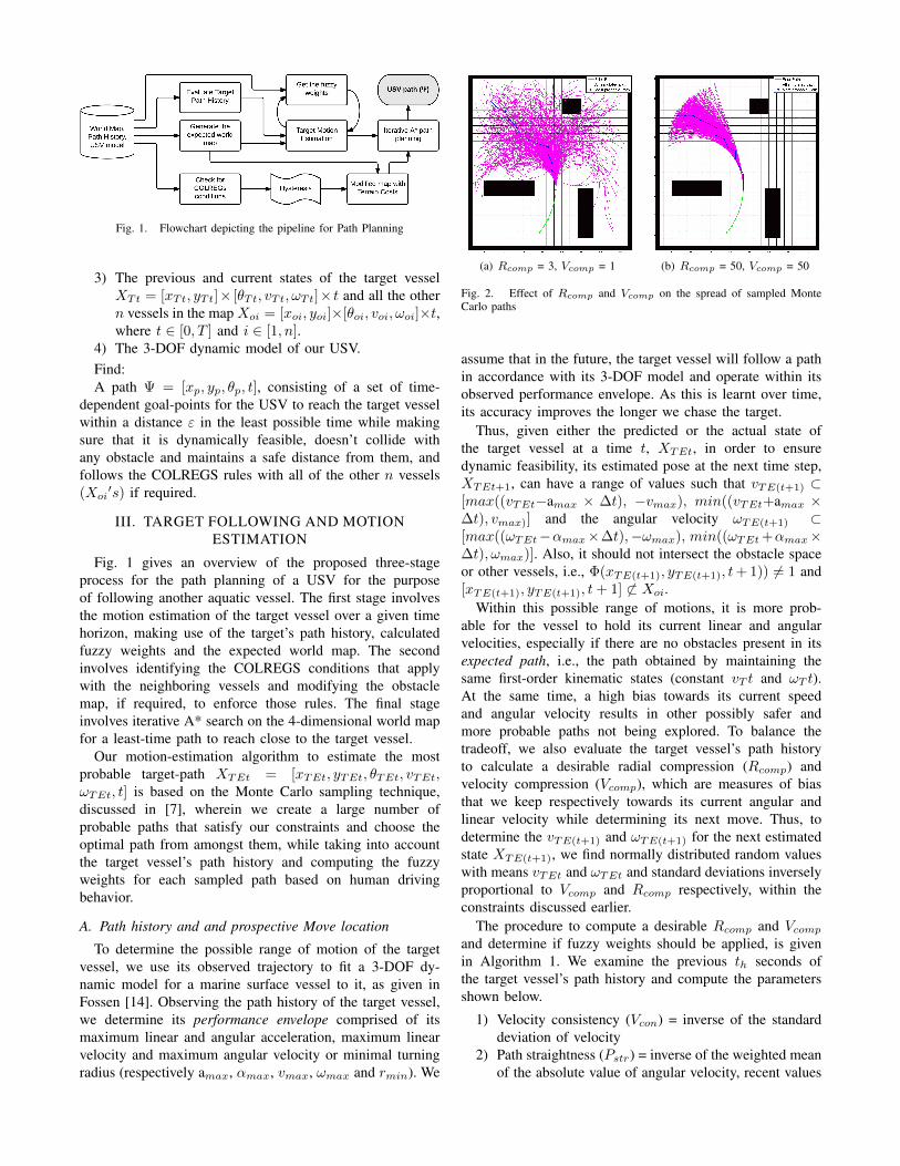
Fig. 1. Flowchart depicting the pipeline for Path Planning

3) The previous and current states of the target vesselXTt = [xTt, yTt]× [θTt, vTt, ωTt]× t and all the othern vessels in the map Xoi = [xoi, yoi]×[θoi, voi, ωoi]×t,where t ∈ [0, T ] and i ∈ [1, n].

4) The 3-DOF dynamic model of our USV.Find:A path Ψ = [xp, yp, θp, t], consisting of a set of time-

dependent goal-points for the USV to reach the target vesselwithin a distance ε in the least possible time while makingsure that it is dynamically feasible, doesn’t collide withany obstacle and maintains a safe distance from them, andfollows the COLREGS rules with all of the other n vessels(Xoi

′s) if required.

III. TARGET FOLLOWING AND MOTIONESTIMATION

Fig. 1 gives an overview of the proposed three-stageprocess for the path planning of a USV for the purposeof following another aquatic vessel. The first stage involvesthe motion estimation of the target vessel over a given timehorizon, making use of the target’s path history, calculatedfuzzy weights and the expected world map. The secondinvolves identifying the COLREGS conditions that applywith the neighboring vessels and modifying the obstaclemap, if required, to enforce those rules. The final stageinvolves iterative A* search on the 4-dimensional world mapfor a least-time path to reach close to the target vessel.

Our motion-estimation algorithm to estimate the mostprobable target-path XTEt = [xTEt, yTEt, θTEt, vTEt,ωTEt, t] is based on the Monte Carlo sampling technique,discussed in [7], wherein we create a large number ofprobable paths that satisfy our constraints and choose theoptimal path from amongst them, while taking into accountthe target vessel’s path history and computing the fuzzyweights for each sampled path based on human drivingbehavior.

A. Path history and and prospective Move location

To determine the possible range of motion of the targetvessel, we use its observed trajectory to fit a 3-DOF dy-namic model for a marine surface vessel to it, as given inFossen [14]. Observing the path history of the target vessel,we determine its performance envelope comprised of itsmaximum linear and angular acceleration, maximum linearvelocity and maximum angular velocity or minimal turningradius (respectively amax, αmax, vmax, ωmax and rmin). We

(a) Rcomp = 3, Vcomp = 1 (b) Rcomp = 50, Vcomp = 50

Fig. 2. Effect of Rcomp and Vcomp on the spread of sampled MonteCarlo paths

assume that in the future, the target vessel will follow a pathin accordance with its 3-DOF model and operate within itsobserved performance envelope. As this is learnt over time,its accuracy improves the longer we chase the target.

Thus, given either the predicted or the actual state ofthe target vessel at a time t, XTEt, in order to ensuredynamic feasibility, its estimated pose at the next time step,XTEt+1, can have a range of values such that vTE(t+1) ⊂[max((vTEt−amax × ∆t), −vmax), min((vTEt+amax ×∆t), vmax)] and the angular velocity ωTE(t+1) ⊂[max((ωTEt−αmax×∆t),−ωmax), min((ωTEt +αmax×∆t), ωmax)]. Also, it should not intersect the obstacle spaceor other vessels, i.e., Φ(xTE(t+1), yTE(t+1), t+ 1)) 6= 1 and[xTE(t+1), yTE(t+1), t+ 1] 6⊂ Xoi.

Within this possible range of motions, it is more prob-able for the vessel to hold its current linear and angularvelocities, especially if there are no obstacles present in itsexpected path, i.e., the path obtained by maintaining thesame first-order kinematic states (constant vT t and ωT t).At the same time, a high bias towards its current speedand angular velocity results in other possibly safer andmore probable paths not being explored. To balance thetradeoff, we also evaluate the target vessel’s path historyto calculate a desirable radial compression (Rcomp) andvelocity compression (Vcomp), which are measures of biasthat we keep respectively towards its current angular andlinear velocity while determining its next move. Thus, todetermine the vTE(t+1) and ωTE(t+1) for the next estimatedstate XTE(t+1), we find normally distributed random valueswith means vTEt and ωTEt and standard deviations inverselyproportional to Vcomp and Rcomp respectively, within theconstraints discussed earlier.

The procedure to compute a desirable Rcomp and Vcomp

and determine if fuzzy weights should be applied, is givenin Algorithm 1. We examine the previous th seconds ofthe target vessel’s path history and compute the parametersshown below.

1) Velocity consistency (Vcon) = inverse of the standarddeviation of velocity

2) Path straightness (Pstr) = inverse of the weighted meanof the absolute value of angular velocity, recent values

getting more weight3) Curvature consistency (Ccon) = inverse of the standard

deviation of the angular velocity4) Net angular difference (∆θth) = angle moved in the

last th time steps

Algorithm 1 Evaluating path history1: Initialize Rcomp to 12: Use fuzzy weights as default3: Vcomp = max(1,min(α1 × Vcon, Vcomp max))4: if Pstr > β1 then5: if no obstacle in expected path then6: Rcomp = max(1,min(α2 × Pstr, Rcomp max))7: end if8: else if Ccon > β2 then9: if no obstacle in expected path then

10: Rcomp = max(1,min(α3 × Ccon, Rcomp max))11: end if12: if ∆θth < β3 then13: Don’t use fuzzy weights14: end if15: end if

In Algorithm 1, α1 controls the velocity compressionas a function of velocity consistency, while α2 and α3

respectively control the radial compression according tothe path’s straightness and curvature consistency, within thelimits of [1, Vcomp max] and [1, Rcomp max]. β1, β2 and β3respectively control the margins for a path to be classified asa straight path, a path with consistent angular velocity, anda path with high net angular difference. Fig. 2(a) and 2(b)shows the effects of varying Rcomp and Vcomp on the spreadof sampled Monte Carlo paths.

B. Fuzzy Weights

Along with generating probable and dynamically-feasiblepaths for the target vessel, in most cases we appoint a fuzzyweight to each of the paths generated through the Monte-Carlo sampling so that a path resembling human drivingbehavior gets higher weight, leading to anthropomorphicmotion prediction. The assumptions made here about thehuman driving are that in a non-evasive target followingscenario:• Coming back very close to the starting location is

unlikely• Suddenly making a large turn and ending up with a very

different angle from the original heading is unusual• Making too many erratic turns is not expected• Maintaining a safe distance from obstacles is expectedThe fuzzy weights (wi) assigned to each of the generated

paths are calculated by a Mamdani’s fuzzy system [15] basedon the parameters depicted in Fig. 3, developed along thelines of the above assumptions.

C. Optimal Path Estimation

Once all paths are generated through the Monte-Carlosampling and their fuzzy weights calculated, the most prob-

Fig. 3. Parameters for fuzzy weights

able path for the target vessel in the discrete space iscalculated for every time interval using Algorithm 2 be-low. At every time interval, the [xTE(t+1), yTE(t+1)] forthe next state must be in a region within a maximumradius of (vTEt+amax × ∆t) × ∆t and a minimum radiusof (vTEt−amax × ∆t) × ∆t from [xTEt, yTEt]. Similarly,θTE(t+1) must lie between (ωTEt + αmax ×∆t)×∆t and(ωTEt − αmax × ∆t) × ∆t, thereby leading to additionalweights w2.

Algorithm 2 Optimal Path Estimation1: Input: Current position of the target at timet0: XTt0, all Monte-Carlo paths XTit =[xTit, yTit, θTit, vTit, ωTit, t] for t ∈ [t1, (t1 + tmax)],i ∈ [1, number of paths] and fuzzy weights wi

2: Output: Expected target path XTEt =[xTEt, yTEt, θTEt, vTEt, ωTEt, t]

3: Procedure:4: for all t← t1, (t1 + tmax) do5: Define P as a zero matrix of the size of map×4,

where Pxyj = P (round(xTit), round(yTit), j)6: for all i← 1, number of paths do7: Pxy2 = (Pxy2 × Pxy1 + θTit ×wi)/(Pxy1 +wi)8: Pxy3 = (Pxy3 × Pxy1 + vTit ×wi)/(Pxy1 +wi)9: Pxy4 = (Pxy4 ×Pxy1 + ωTit ×wi)/(Pxy1 +wi)

10: Pxy1 = Pxy1 + wi

11: end for12: Smooth P by applying a 2D Gaussian kernel on all

4 layers of it13: Determine the weights w2 from XTE(t−1)14: Set P2 as the 1st layer of P × w2

15: Find the grid in P2 with highest value and set it as[xTEt, yTEt]

16: Set θTEt, vTEt and ωTEt as P (xTEt, yTEt, 2),P (xTEt, yTEt, 3) and P (xTEt, yTEt, 4) respectively

17: end for18: return [xTEt, yTEt, θTEt, vTEt, ωTEt]

Fig. 4. Figure depicting the possible COLREGS and critical cases, andthe appropriate avoidance behavior with Artificial Terrain Costs shown inbrown

IV. COLREGS IMPLEMENTATION

A. COLREGS Cases

The official COLREGS rulebook [3] specifies a total of 38rules to be followed in different circumstances for preventionof collision between marine vehicles. Many rules serve onlyas guidance; in this paper, we address the 4 main cases:Head-on collision, overtaking, crossing from the left andcrossing from the right, illustrated in Fig. 4.

To determine if the USV is about to collide with anothervessel, we use the Closest Point of Approach (CPA) test[16] with every other vessel in proximity to determine upto a particular time horizon tmax, the closest that eachvessel is expected to come to the USV (dCPA tmax

). Weapply a COLREGS avoidance maneuver if dCPA tmax

isless than a threshold distance dCOLREGS . If the COLREGScondition applies with a certain vessel, we identify whichscenario it belongs to according to their current states andexpected relative positions at the CPA, before making theavoidance maneuver. To add stability to the identified ruleand ensure that the USV’s maneuver is understandable tothe neighboring vessels, hysteresis is added. A good way toidentify the appropriate rules and to apply hysteresis is givenin [9].

If the vessel is already extremely close to the USV(dt0 < dcritical), the collision is treated as a critical caseand the avoidance strategy is executed without considerationto the COLREGS rules with those specific vessels. Suchscenarios can arise when the other vessel fails to complywith COLREGS or intentionally comes very close to theUSV, as in an adversarial scenario.

B. Implementing the obstacle avoidance maneuver

To incorporate COLREGS into the A* path-planning, wemodify the obstacle map Φ ⊆ R2 × T by introducingnew obstacles and terrain cost, as shown in Fig. 4. Bycreating Artificial Terrain Costs in the obstacle map foreach vessel (Xoi = [xoi, yoi] × [θoi, voi, ωoi, t]) throughits planning horizon, the USV avoids crossing them fromcertain directions. The net obstacle map Φ is calculated bytaking the maximum cost from the obstacle map of eachvessel Xoi. The Artificial Terrain Costs are non-lethal, sovarying them will change how strongly the COLREGS rulesare followed. If the Terrain Costs are set to maximum, theplanner would never be able to plan a path over them, which

may lead to inability to find a path if there are multiplevessels surrounding the USV.

In the critical case, Artificial Terrain Costs are insteadcreated directly in the direction of the vessel’s velocity up toa distance of voi/v plus a margin to ensure that a collisiondoes not occur. Similarly, Artificial Terrain Costs are alsocreated around other static and dynamic obstacles so thatthe USV does not get very close to them.

V. DYNAMIC PATH PLANNING

The path planning for the USV is done through iterativeA* heuristic path planning in 4-dimensional R2×Θ×T spaceto find the shortest path in time, while also maintaining a safedistance from the obstacles. Paths are appropriately penalizeddepending on the number of turns required, how close to anobstacle they get, degree of traversal over high-cost terrain,and their total length. To enforce dynamic feasibility on thecomputed paths, the next move from the current state is onlychosen from a set of options that satisfies the constraintsgiven by the 3-DOF model [14] of our USV.

The paths are iteratively computed from the current poseof the USV [x, y, θ, v] as the starting point to the successiveestimated states of the target vessel [xTEt, yTEt] as the goalpoints. At the time the target vessel is expected to reach thegoal point, if the USV is expected to be within a distanceof ε from it, the computed path is appointed as the USV’splanned path (Ψ = [xp, yp, θp, t]). Otherwise the goal pointis selected as the next estimated state of the target vessel andthe same process is repeated until we reach the last estimatedstate in the planning horizon.

VI. RESULTS

A. Simulation Results

To compare the efficiency of the developed motion es-timation algorithm with previous methods and to checkthe implementation of the COLREGS rules with nearbyvessels, simulations were carried out in a total of 15 differentenvironments, 5 each with no obstacles, static obstaclesand dynamic obstacles. The environments were created torepresent a diverse set of real-world scenarios which theUSV may encounter in its application, ranging from open-sea conditions with high-speed chase to dense harbor-likescenarios with many static and dynamic obstacles. The USV,while following a target vessel executing both evasive andnon-evasive manoeuvres, also followed the COLREGS ruleswith between 1-3 civilian vessels.

Table 1 shows the averaged comparative result for targetfollowing with the following motion estimations: (1) PurePursuit (PP), where the ownship is steered directly in thedirection of the target vessel’s current position. (2) ConstantBearing (CB), where the ownship is steered to the CPAgiven by the vessel’s present position, bearing and speed, andownship’s desired chase speed. (3) Simple Monte Carlo (MC)(as presented in [7]). And (4) the proposed Modified Monte-Carlo (M-MC) based motion estimation, all with PP as thebase-line. In the no obstacles scenarios, the proposed M-MCmotion estimation does no better than the CB estimation, as

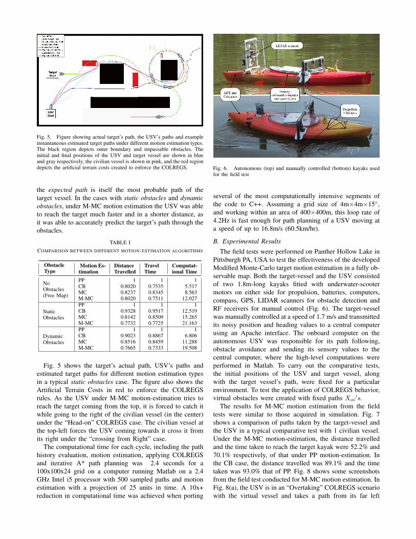
Fig. 5. Figure showing actual target’s path, the USV’s paths and exampleinstantaneous estimated target paths under different motion estimation types.The black region depicts outer boundary and impassable obstacles. Theinitial and final positions of the USV and target vessel are shown in blueand gray respectively, the civilian vessel is shown in pink, and the red regiondepicts the artificial terrain costs created to enforce the COLREGS.

the expected path is itself the most probable path of thetarget vessel. In the cases with static obstacles and dynamicobstacles, under M-MC motion estimation the USV was ableto reach the target much faster and in a shorter distance, asit was able to accurately predict the target’s path through theobstacles.

TABLE ICOMPARISON BETWEEN DIFFERENT MOTION-ESTIMATION ALGORITHMS

ObstacleType

Motion Es-timation

DistanceTravelled

TravelTime

Computat-ional Time

NoObstacles(Free Map)

PP 1 1 1CB 0.8020 0.7535 5.517MC 0.8237 0.8345 8.563M-MC 0.8020 0.7511 12.027

StaticObstacles

PP 1 1 1CB 0.9328 0.9517 12.519MC 0.8142 0.8509 15.265M-MC 0.7732 0.7725 21.163

DynamicObstacles

PP 1 1 1CB 0.9023 0.8867 6.806MC 0.8516 0.8459 11.288M-MC 0.7665 0.7333 19.508

Fig. 5 shows the target’s actual path, USV’s paths andestimated target paths for different motion estimation typesin a typical static obstacles case. The figure also shows theArtificial Terrain Costs in red to enforce the COLREGSrules. As the USV under M-MC motion-estimation tries toreach the target coming from the top, it is forced to catch itwhile going to the right of the civilian vessel (in the center)under the “Head-on” COLREGS case. The civilian vessel atthe top-left forces the USV coming towards it cross it fromits right under the “crossing from Right” case.

The computational time for each cycle, including the pathhistory evaluation, motion estimation, applying COLREGSand iterative A* path planning was 2.4 seconds for a100x100x24 grid on a computer running Matlab on a 2.4GHz Intel i5 processor with 500 sampled paths and motionestimation with a projection of 25 units in time. A 10x+reduction in computational time was achieved when porting

Fig. 6. Autonomous (top) and manually controlled (bottom) kayaks usedfor the field test

several of the most computationally intensive segments ofthe code to C++. Assuming a grid size of 4m×4m×15◦,and working within an area of 400×400m, this loop rate of4.2Hz is fast enough for path planning of a USV moving ata speed of up to 16.8m/s (60.5km/hr).

B. Experimental Results

The field tests were performed on Panther Hollow Lake inPittsburgh PA, USA to test the effectiveness of the developedModified Monte-Carlo target motion estimation in a fully ob-servable map. Both the target-vessel and the USV consistedof two 1.8m-long kayaks fitted with underwater-scootermotors on either side for propulsion, batteries, computers,compass, GPS, LIDAR scanners for obstacle detection andRF receivers for manual control (Fig. 6). The target-vesselwas manually controlled at a speed of 1.7 m/s and transmittedits noisy position and heading values to a central computerusing an Apache interface. The onboard computer on theautonomous USV was responsible for its path following,obstacle avoidance and sending its sensory values to thecentral computer, where the high-level computations wereperformed in Matlab. To carry out the comparative tests,the initial positions of the USV and target vessel, alongwith the target vessel’s path, were fixed for a particularenvironment. To test the application of COLREGS behavior,virtual obstacles were created with fixed paths Xoi

′s.The results for M-MC motion estimation from the field

tests were similar to those acquired in simulation. Fig. 7shows a comparison of paths taken by the target-vessel andthe USV in a typical comparative test with 1 civilian vessel.Under the M-MC motion-estimation, the distance travelledand the time taken to reach the target kayak were 52.2% and70.1% respectively, of that under PP motion-estimation. Inthe CB case, the distance travelled was 89.1% and the timetaken was 93.0% that of PP. Fig. 8 shows some screenshotsfrom the field test conducted for M-MC motion estimation. InFig. 8(a), the USV is in an “Overtaking” COLREGS scenariowith the virtual vessel and takes a path from its far left

Fig. 7. Compilation of the paths taken by the USV to follow the targetvessel in the field test under different target motion-estimations whileobeying COLREGS with a civilian vessel (shown in pink). The region withArtificial Terrain Costs for M-MC case is shown in red

(a) Overtaking (b) Head-on

Fig. 8. Screenshots from the test showing the COLREGS avoidancemanoeuvre for the USV (in blue) with the civilian vessel (in pink) to followthe target vessel (in gray). The regions with Artificial Terrain Costs areshown in red

side, keeping sufficient margin. In Fig. 8(b), the USV is in a“Head-on” collision with the virtual vessel and hence plansa path from its starboard side.

VII. CONCLUSIONS AND FUTURE WORK

We present accurate and anthropomorphic motionestimation-based autonomous target-following by an Un-manned Surface Vehicle while following the COLEGS ruleswith nearby marine vessels. The increased accuracy inmotion-prediction is achieved by continuously learning thetarget vessel’s navigational behavior from its path historywithout any prior knowledge and ensuring that the pre-dicted path resembles human driving behavior by the use offuzzy weights. This integrated single-stage path planning isachieved by fusing the COLREGS rules directly with the dy-namic A* heuristic path-planning around dynamic obstaclesby imposing Artificial Terrain Costs, while also consideringthe kinematic and dynamic constraints of the USV. Wehave demonstrated that this can be achieved robustly andwithin practical levels of computation, even in situationswith multiple civilian vessels and dynamic obstacles, throughcomparative tests with other motion-estimation methods in

simulation and field experiments.Our future goals are to learn the maneuvering behavior of

the target-vessel around obstacles and its evasive maneuverthrough the use of reinforcement learning. We plan to reducethe computational time for the planner by making use ofvariable grid size with a higher resolution near the obstacles.We also intend to test our approach on a larger body of waterwhile working at higher speeds and without having the targetvessel to broadcast its state.

ACKNOWLEDGMENT

This research was supported by the National ScienceFoundation award IIS1124941. Thanks to Weilong Song,Chiyu Dong and Hang Cui for help in performing the fieldtests.

REFERENCES

[1] R. J. Yan, S. Pang, H. B. Sun, and Y. J. Pang, “Development andmissions of unmanned surface vehicle,” Journal of Marine Scienceand Application 9.4 (2010): pp. 451-457.

[2] S. Campbell, W. Naeem, and G. W. Irwin, “A review on improving theautonomy of unmanned surface vehicles through intelligent collisionavoidance manoeuvres,” Annual Reviews in Control 36.2 (2012): 267-283.

[3] U.S. Department Of Homeland Security, “U.S. Coast Guard, Naviga-tion Rules,” Paradise Cay Publications, 2010.

[4] Y. Kuwata, M. Wolf, D. Zarzhitsky, and T. Huntsberger, “Safe Mar-itime Navigation with COLREGS Using Velocity Obstacles,” Proc.IEEE/RSJ International Conference on Intelligent Robots and Systems(IROS’11), 2011.

[5] P. Svec, B. C. Shah, I. R. Bertaska, J Alvarez, A J. Sinisterra,K. Ellenrieder, M. Dhanak, and S. K. Gupta, “Dynamics-AwareTarget Following for an Autonomous Surface Vehicle Operating underCOLREGS in Civilian Traffic,” Intelligent Robots and Systems (IROS),2013 IEEE/RSJ.

[6] M. Benjamin, J. Curcio, and P. Newman, “Navigation of UnmannedMarine Vehicles in Accordance with the Rules of the Road,” inProceedings of the IEEE International Conference on Robotics andAutomation, 2006.

[7] S.-M. Lee, K.-Y. Kwon, and J. Joh, “A Fuzzy Logic for AutonomousNavigation of Marine Vehicles Satisfying COLREG Guidelines,” In-ternational Journal of Control Automation and Systems 2 (2004): 171-181.

[8] L. P. Perera, J. P. Carvalho, and C. G. Soares, “Autonomous guidanceand navigation based on the COLREGS rules and regulations ofcollision avoidance,” in Proceedings of the International WorkshopAdvanced Ship Design for Pollution Prevention 2009, pp. 205-216.

[9] M. Breivik, V. E. Hovstein, and T. I. Fossen, “Straight-line targettracking for unmanned surface vehicles,” Modeling, Identification andControl 29.4 (2008): 131-149.

[10] M. Bibuli, M. Caccia, L. Lapierre, and G. Bruzzone, “Guidanceof unmanned surface vehicles: Experiments in vehicle following,”Robotics & Automation Magazine, IEEE, 1999.

[11] T.H. Chung, G.A. Hollinger, and V. Isler, “Search and pursuit-evasionin mobile robotics,” Autonomous Robots, pages 1-18, 2011.

[12] P. Svec and S. K. Gupta, “Automated synthesis of action selectionpolicies for unmanned vehicles operating in adverse environments,”Autonomous Robots 2012, Volume 32, Issue 2, pp. 149-164.

[13] P. Svec, A. Thakur, B. C. Shah, and S.K. Gupta, “Target following withmotion prediction for unmanned surface vehicle operating in clutteredenvironments,” Autonomous Robots, 2013.

[14] T. I. Fossen, “Guidance and control of ocean vehicles,” in Wiley,Chicester, England, 1994.

[15] J. H. Lilly, “Mamdani Fuzzy Systems,” Fuzzy Control and Identifica-tion (2010): 27-45.

[16] S. Arumugam, and C. Jermaine, “Closest-point-of-approach join formoving object histories,” Data Engineering, 2006. ICDE’06. Proceed-ings of the 22nd International Conference on. IEEE, 2006.