collapse of showa bridge during 1964 niigata earthquake… · bhattacharya et al. on “collapse of...

Bhattacharya et al. on “Collapse of Showa Bridge during 1964 Niigata Earthquake: A reappraisal on the failure

mechanisms”

Collapse of Showa Bridge during 1964 Niigata Earthquake: A reappraisal on the failure mechanisms

AUTHORS AND AFFILIATIONS:

S. Bhattacharya1*, K. Tokimatsu2, K.Goda3 R. Sarkar4 and M. Shadlou5 and

M.Rouholamin6

1 Chair in Geomechanics, University of Surrey, U.K.

2 Professor, Tokyo Institute of Technology, Japan

3 Senior Lecturer, University of Bristol, U.K

4 Asst Professor, Malaviya National Institute of Technology, Jaipur, India

5 PhD Student, University of Bristol, U.K.

6 PhD Student, University of Surrey, U.K.

Key words: Showa Bridge, Niigata earthquake, natural frequency, collapse, liquefaction

* Address for correspondence: Professor Subhamoy Bhattacharya Department of Civil and Environmental Engineering, University of Surrey, Thomas Telford Building, Guildford, Surrey GU2 7XH Phone number: 01483 689534 E-Mail: [email protected]

mailto:[email protected]


mechanisms”

ABSTRACT

Collapse of Showa Bridge during the 1964 Niigata earthquake has been, throughout the years, an

iconic case study for demonstrating the devastating effects of liquefaction. Inertial forces during

the initial shock (within the first 7seconds of the earthquake) or lateral spreading of the surrounding

ground (which started at 83 seconds after the start of the earthquake) cannot explain the failure of

Showa Bridge as the bridge failed at about 70seconds following the main shock and before the

lateral spreading of the ground started. In this study, quantitative analysis is carried out for the

various failure mechanisms that may have contributed to the failure. The study shows that at about

70 seconds after the onset of the earthquake, the increased natural period of the bridge (due to the

elongation of unsupported length of the pile owing to soil liquefaction) tuned with the period of

the liquefied ground causing resonance between the bridge and the ground motion. This tuning

effect (resonance) caused excessive deflection at the pile head adequate to unseat the bridge deck

from the supporting pier and thereby initiating the collapse of the bridge.


mechanisms”

1.0 INTRODUCTION

1.1 Importance of the study

The collapse of Showa Bridge (see Figure 1 for location with respect to North-South direction,

Figure 2 for a photograph of the collapse and Figure 3 for a schematic diagram) during the 1964

Niigata earthquake features in many publications as an iconic example of the detrimental effects of

liquefaction induced lateral spreading of the ground, see for example Hamada and O’Rourke (1992),

Kramer (1996), Bhattacharya (2003), Bhattacharya et al. (2005), Yoshida et al. (2007), Bhattacharya

et al. (2008) and Bhattacharya and Tokimatsu (2013). It was generally believed that lateral spreading

was the cause of failure of the bridge (Hamada and O’Rourke, 1992). This hypothesis is based on

the reliable eye witness that the bridge failed 1 to 2 minutes after the earthquake started which

clearly ruled out the possibility that inertia, in the initial strong shaking, was the contributor to the

collapse.

However, Bhattacharya (2003), Bhattacharya et al .(2005), Bhattacharya and Madabhushi

(2008) reanalysed the bridge and showed that lateral spreading hypothesis cannot explain the failure

of the bridge. They argued: (a) had the cause of failure been due to lateral spreading, as suggested,

the piers (see Pier P5 and Pier P6 in Figure 3) should have displaced identically in the direction of

the slope. (b) the piers close to the riverbanks did not fail, where the lateral spreading was seen to

be severe. This conjecture was later confirmed by the study carried out by Yoshida et al. (2007)

who suggested that lateral spreading of the surrounding ground started after the bridge had

collapsed. Towhata et al. (1992) indicated that the permanent ground displacements of liquefied

strata are strongly affected by topographical and geological conditions, and are not explicit

functions of earthquake time series. Kerciku et al. (2008) showed that liquefied soil under the middle

of the bridge (under pier P5 and P6) was already at its lowest positions of potential energy and

would not be expected to flow. All the above circumstantial evidences and arguments suggest that

lateral spreading may not be the cause for the collapse of Showa bridge.


mechanisms”

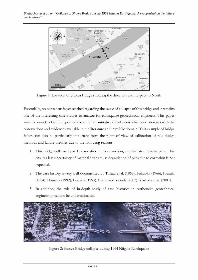
Figure 1: Location of Showa Bridge showing the direction with respect to North

Essentially, no consensus is yet reached regarding the cause of collapse of this bridge and it remains

one of the interesting case studies to analyze for earthquake geotechnical engineers. This paper

aims to provide a failure hypothesis based on quantitative calculations which corroborates with the

observations and evidences available in the literature and in public domain. This example of bridge

failure can also be particularly important from the point of view of calibration of pile design

methods and failure theories due to the following reasons:

1. This bridge collapsed just 15 days after the construction, and had steel tubular piles. This

ensures less uncertainty of material strength, as degradation of piles due to corrosion is not

expected.

2. The case history is very well-documented by Takata et al. (1965), Fukuoka (1966), Iwasaki

(1984), Hamada (1992), Ishihara (1993), Berrill and Yasuda (2002), Yoshida et al. (2007).

3. In addition, the role of in-depth study of case histories in earthquake geotechnical

engineering cannot be underestimated.

Figure 2: Showa Bridge collapse during 1964 Niigata Earthquake

300m


mechanisms”

1.2 Details of the earthquake and the bridge

The Niigata earthquake occurred on the 14th of June 1964 and registered a moment magnitude of

7.6. Located some 55 km from the epicentre, crossing the Shinano River, Showa Bridge (simple

steel girder bridge with pile foundations) was one of the bridges which collapsed as a result of the

earthquake. The total length of the bridge was about 307m. The bridge had 12 composite girders

and its breadth was about 24m. Main span length was about 28m and side span length was about

15m (Fukuoka 1966). Figure 1 shows the location of the bridge. It may be observed that the

longitudinal axis of the bridge is at an angle of 300 North-West. The view of the collapsed Showa

Bridge from the southwest side is shown in Figure 2.

1.3 Post earthquake observations

During the 1964 Niigata earthquake, the bridge site was subjected to extensive liquefaction and

lateral spreading. Reliable eyewitness quoted by Horii (1968) and Hamada and O’Rourke (1992)

along with the progressive damage simulation by Kazama et al. (2008) suggest that the bridge

collapsed 1-2 minutes after the peak ground acceleration (PGA) had ceased. Yoshida et al. (2007)

collated many eye witness statements and established the chronology of the bridge failure. Figure

3 shows a schematic diagram of the collapse of the bridge. Horizontal and vertical deflections of

the pile cap are also indicated in the figure as and l respectively. The sequential failure initiated

when piers P5 and P6 collapsed in opposite directions, accompanied by the fall of girder G5-6

(between P5 & P6) in the river. Immediately afterwards, in a domino effect, girders G6-7, G4-5, G3-4

and G2-3 partially fell in the river. Based on the eye witness reports, Kazama et al. (2008) also

reported that the collapse of the bridge girders proceeded as G5-6→G6-7 →G4-5 →G3-4 →G2-3. As a

result, five of the twelve spans fell off the pile heads in the earthquake.

Figure 3: Schematic diagram of the collapse of the bridge along with the deflections of the pile caps (Iwasaki 1986)

G5-6 G6-7 G7-8 G8-9 G9-10 G10-11 G11-A

G4-5 G3-4 G2-3 G1-2 GA-1


mechanisms”

Figure 4 shows the structural details and soil data for a pile of pier P4 after post earthquake recovery.

On the other hand, Figure 5 shows the deck-pier support arrangement where there is alternating

roller (movable) and pinned (fixed) except for pier P6 where both the supports are roller. Yoshimi

(2003) commented on the lack of redundancy in the structural design of the bridge. It may be noted

from Figure 5 that relative displacement of more than 30cm at the deck level will lead to unseating

of the deck and hence may lead to collapse.

Figure 4: Structural and soil data for a pile of pier P4 (Fukuoka 1966)

Figure 5: Support condition of the bridge at two piers

130cm 130cm

Pier P4

G3-4 G4-5

30cm

Pier P6

G5-6 G6-7

30cm


mechanisms”

1.4 Liquefaction profile

The Showa Bridge was situated in the coastal alluvial plain of the Niigata city which consists of

marine sediments due to current along the Japan sea coast and due to the river or lake deposit

along the Shinano river. The sand was uniformly graded medium sand and its 60 percent diameter

(D60) was about 0.3mm (Fukuoka 1966). Hamada and O'Rourke (1992) estimated the ground

liquefaction profile. As shown in Fig. 6, the soil liquefied to a maximum depth of about 10 m below

the riverbed and to a maximum depth of approximately 5 m below the riverbed near the left

abutment.

Figure 6: Soil liquefaction profile (in grey), Hamada and O'Rourke (1992)

2.0 GROUND ACCELERATION AND DISPLACEMENT

2.1 Recorded ground motion

Fig. 7(a) shows the time history of the acceleration, velocity and displacement recorded at the

basement of a building (Kawagishi-Cho) at a location 1.25 km from the Showa bridge and Figure

7(b) shows the wavelet energy spectrum of the motion. Figure 8 (a) shows the details of the location

of Kawagishi-Cho Apartment House along with the Showa bridge. Figure 8(b) on the other hand

shows typical subsurface soil profile in entire Niigata city inferred from borehole data obtained

before the earthquake. The profile suggests that the soils are primarily sandy down to the depth of

20 to 30m. The figure also shows the lines of equal N values. It may be mentioned that records at

Kawagishi-Cho are the only available strong motion records recovered near Niigata city and the

site was fully liquefied. The next section evaluates the motion to ascertain whether or not this can

be used for studying the Showa Bridge failure.


mechanisms”

Figure 7(a): Recorded acceleration, velocity and displacement time histories, adapted from Kudo et al. (2000). Also in the diagram the time window (65s - 75s) when it is believed the Showa Bridge collapsed is indicated. (http://kyoshin.eri.u-tokyo.ac.jp/SMAD)

Figure 7(b): Wavelet Energy Spectrum of NS component of motion shown in Fig. 7(a)

E-W Component

-1.5

-1.0

-0.5

0.0

0.5

1.0

1.5

Acc

eler

atio

n (

m/s

2)

-0.6

-0.4

-0.2

0.0

0.2

0.4

0.6

Vel

oci

ty (

m/s

)

-0.6

-0.4

-0.2

0.0

0.2

0.4

0.6

Vel

oci

ty (

m/s

)

-0.6

-0.4

-0.2

0.0

0.2

0.4

0.6

0 25 50 75 100 125

Time (s)

Dis

pla

cem

ent

(m)

-0.6

-0.4

-0.2

0.0

0.2

0.4

0.6

0 25 50 75 100 125

Time (s)

Dis

pla

cem

ent

(m)

N-S Component

-1.5

-1.0

-0.5

0.0

0.5

1.0

1.5

Acc

eler

atio

n (

m/s

2) Time frame of

Showa Bridge collapse

Time frame of

Showa Bridge collapse

Energy concentration due to the jolt (initiating the collapse) in the liquefied ground condition

Energy concentration during the initial phase of ground motion

http://kyoshin.eri.u-tokyo.ac.jp/SMAD


mechanisms”

Figure 8(a):Map of Niigata plain showing the Showa Bridge and the Kawagishi-Cho Apartment

House where the ground motion is measured, (Anon, 1966)

Figure 8(b): Typical soil profile in Niigata City along with the Shinano river (JNCEE, 1965)

2.2 Seismological evaluation of the ground motion

The 1964 Niigata earthquake occurred at the convergent boundary between the Eurasian and the

North American plates, having a reverse faulting mechanism. Because the plate interaction at the

boundary was complex and recorded ground motions at distant stations are contaminated by noise,

the fault plane of this event (whether the fault plane was west-dipping or east-dipping) has not yet

been unanimously agreed by seismologists (e.g. Abe, 1975; Shiba and Uetake, 2011; Hurukata and

Harada, 2013). Recently, Shiba and Uetake (2011) have proposed a west-dipping fault plane,

whereas Hurukata and Harada (2013) have suggested an east-dipping fault plane. In this study, the

two alternatives by Shiba and Uetake (2011) and Hurukata and Harada (2013) (i.e. east-dipping and

west-dipping fault planes) are adopted to examine the directivity of seismic wave propagation and


mechanisms”

to calculate the distance between a site of interest (Showa Bridge and Kawagishi-Cho) and the

rupture source.

Figure 9 shows the locations of the two fault planes for the 1964 Niigata earthquake: the

fault plane 1 is based on Shiba and Uetake (2011) – i.e. west-dipping, while the fault plane 2 is

based on Hurukata and Harada (2013) – i.e. east-dipping. Note that the fault plane 1 is steeper than

the fault plane 2 (60 degrees versus 34 degrees). In the figure, the locations of Showa Bridge

(37.9128N, 139.0427E) and Kawagishi-Cho (37.9093N, 139.0294E) are also indicated. For the fault

plane 1, the shortest rupture distances to Showa Bridge and Kawagishi-Cho are calculated as 14.5

and 15.6 km, respectively. For the fault plane 2, the shortest rupture distances to Showa Bridge

and Kawagishi-Cho are calculated as 17.0 and 17.5 km, respectively. The distance between Showa

Bridge and Kawagishi-Cho is 1.25 km. From Figure 9, it is clear that the Showa Bridge and

Kawagishi-Cho sites share the similar wave propagation path, noting that the rupture process of

the 1964 Niigata earthquake occurred bilaterally from the hypocentre (Shiba and Uetake, 2011).

Thus the directions of rupture propagation and seismic wave propagation coincide for the southern

half of the fault plane.

Figure 9. Locations of two fault planes for the 1964 Niigata earthquake

As mentioned earlier, very important ground motion time-history data were recorded at the

Kawagishi-Cho apartment building, where severe liquefaction was observed (and consequently,

multiple apartment buildings toppled down because of liquefaction-induced instability at the

building foundation). A map of Showa Bridge and Kawagishi-Cho is shown in Figure 8(a) and


mechanisms”

similar extensive liquefaction was observed at/near Showa Bridge (Yoshida et al. 2007). Near

ground surface soil profiles in Niigata City (top 5 to 15 m) are typically characterised by (liquefiable)

soft sandy deposits (typical N values are less than 10), which are formed by Shinano River over

many years (see Figure 8(b)). As noted by Kudo et al. (2000), in Niigata City, the basin effects are

significant due to fluvial river deposits. Based on this information, it is reasonable to consider that

surface soil profiles at the Kawagishi-Cho and Showa Bridge sites are broadly similar in terms of

surface site amplification and liquefaction potential.

Figure 10 shows the acceleration and velocity time-history data at Kawagishi-Cho. As noted

by Kudo et al. (2000), the initial part of the record (before 7 seconds) is mainly due to P-wave,

while the latter part is affected by S-wave and surface waves. They also indicated that ground

motions between 7 and 12 seconds contain long-period component (having the peak spectral value

around 5-6 seconds), and these can be attributed to surface waves significantly affected by the

Niigata basin. According to Kudo et al. (2000), the liquefaction triggering had stated around 12

seconds. To visually inspect the effects of liquefaction triggering in the top surface soil, response

spectra of the NS and EW components of the Kawagishi-Cho record are computed (damping ratio

= 5%) for the entire time-history data and for the first 12 seconds of the data (i.e. focusing on the

part that is not significantly affected by liquefaction). The results are shown in Figure 11. The

comparison of response spectra indicates that the short-period content of ground motions is

relatively low despite the fact that the large earthquake occurred at short distance (note: although

the shortest rupture distance is about 15-20 km, the hypocentral distance is about 55-60 km;

according to Shiba and Uetake (2011), the main asperity is located near the hypocenter). The main

reason for the low short-period response spectra is attributed to significant site/basin effects.

Figure 11 also shows that the response spectra for the entire record and the first 12 seconds are

similar for vibration periods less than 5 seconds; for the NS component, the inclusion of the time-

history data affected by liquefaction results in additional peak at around 6-7 seconds. It is reminded

that the 1964 Niigata earthquake occurred at the off-shore plate boundary and the shortest source-

to-site distances for Niigata City (where Kawagishi-Cho and Showa Bridge are located) are about

15-20 km. Therefore, it is unclear whether ‘typical near-fault motion’ condition (for shallow

continental crustal earthquakes) is applicable to this case. In other words, it is not straightforward

to separate the directivity effects and site/basin effects in the recorded ground motions at

Kawagishi-Cho. The next section therefore explores the variability of ground motion in greater

details.


mechanisms”

Figure 10. Acceleration and velocity time-history data at Kawagishi-Cho.

Figure 11: Response spectra of the ground motion record at Kawagishi-Cho.

2.3 Variability of Ground Motions at Kawagishi-Cho and Showa Bridge Site

Variability of ground motions at nearby sites is investigated for the case of Kawagishi-Cho and

Showa Bridge during the 1964 Niigata earthquake. The analysis presented herein is focused on the

ground motion intensities during the initial part of the ground motions (i.e. prior to liquefaction

triggering), to which ground motion models are applicable. In addition, several key considerations

that are unique to the problem are noted:


mechanisms”

(a) Firstly, the wave propagation paths from the source region to Kawagishi-Cho/Showa Bridge

are considered to be similar based on the relative locations of the two sites and the source rupture

zone (Figure 9);

(b) Secondly, the near surface site profiles at the two locations are broadly similar based on the

surveyed soil profile (Figure 8(b)) and the fact that major liquefaction was actually observed at the

two locations (Yoshida et al. 2007).

To estimate the ground motion intensity at Showa Bridge given the recorded motion at Kawagishi-

Cho, a prediction tool that is based on statistical analysis of ground motion data is adopted – i.e.

spatial correlation model of a ground motion parameter for a given scenario. The tool was

developed by Goda and Atkinson (2010) and Goda (2011), calibrated using extensive actual ground

motion data around the world; notably, the dataset analysed by Goda (2011) includes the 2004 and

2007 Chuetsu-(Oki) earthquakes, which occurred in the same region.

The procedure of the estimation is briefly mentioned. A typical ground motion prediction equation

can be expressed as: ),,,(log 3010 VRMfY ) where Y represents the ground motion

parameter of interest (e.g. PGA and spectral acceleration); ),,,( 30 VRMf is the median prediction

model as functions of magnitude M, distance R, site parameter VS30, and other parameters ; is

the intra-event residual. It is noted that the above equation is focused upon a single event (rather

than multiple events, as in the typical cases for ground motion models; note: the result is valid for

both cases). In this model, Y is modelled as lognormal variate with median ),,,( 30 VRMf

(described by several physical parameters) and error term . is assumed to be normally

distributed with zero mean and variance of 2

. If one is interested in estimating a ground motion

parameter at an unobserved site based on the ground motion parameter at a nearby observed site,

an extended version of the above ground motion model can be employed. One notable aspect in

this estimation is the consideration of spatial correlation of ground motion parameters at nearby

sites. The correlation of at two locations can be given by the intra-event spatial correlation

),( T , where is the separation distance between two sites and T is the vibration period. The

details of ),( T can be found in Goda and Atkinson (2010) and Goda (2011). Now, consider

that the ground motion parameter is available at Kawagishi-Cho and based on this information,

the ground motion parameter at Showa Bridge is estimated. For the bivariate case, the error term

at Showa Bridge is characterised by the normal distribution with mean equal to

Cho-Kawagishi),( T and variance equal to 22)],([1( T . With this information, one can


mechanisms”

easily assess the confidence interval of the ground motion parameter at Showa Bridge given the

observed ground motion at Kawagishi-Cho. The key parameters in the estimation procedure are

),( T and 2

.

Another important information is the intra-event spatial correlation and to provide the empirical

estimates of the correlation using extensive ground motion data worldwide, comparison of spatial

correlations for the well-recorded 41 earthquakes is presented in Figure 12 (Goda, 2011). In

addition, the results for the two relevant regional earthquakes are shown in Figure 13. The result

shown in Figures 12 and 13 is the estimated intra-event spatial correlation at the shortest separation

distance ( ≈ 2.5 km; 5 km bin size). This separation distance is the closest one can go (note: to

estimate the spatial correlation coefficient for the closest separation distance bin, a sufficient

number of data points (more than 50) was used (thus the estimates are relatively stable in a statistical

sense). The results shown in Figures 12 and 13 suggest that ),( T at the separation distance of

0-5 km is about 0.4-0.9; this variability is attributed to vibration period and different earthquakes.

As the vibration period increases, ),( T increases. For the considered case, the relevant

vibration period is longer than 3 seconds (note: the correlation model is available up to 5 seconds).

For this period range, ),( T is between 0.7 and 0.9 (typical value is 0.8).

Values of the intra-event standard deviation of well-recorded earthquakes range from

0.15 and 0.4 (log 10 base); see Goda (2011). On average, 3.0 is a reasonable choice. In

particular, for the two relevant earthquakes in Niigata region, i.e. 2004 and 2007 Chuetsu(-Oki)

earthquakes, values of are about 0.3-0.33. The mentioned values of is based on ground

motion data distributed over a wide area (for a given event), while more detailed investigations that

are focused upon specific site-path combinations suggest that the intra-event standard deviation is

much less than the overall estimate. Specifically, the study by Morikawa et al. (2008) indicated that

the reduction of can be as large as 60-70% (i.e. for the specific site-path combination

becomes about (as low as) 0.1). Because the specific site-path is applicable to the situation discussed

in this note, a reduction of can be justified; as a typical value, 50% reduction is considered in

the following part.

Using the representative parameter values of ),( T and (i.e. 0.8 and 0.15), the error term at

Showa Bridge is characterised by the normal distribution with mean equal to 0.8 ChoKawagishi and

variance equal to 0.36×0.152 = 0.0081 (i.e. intra-event standard deviation is 0.09 (log10 base)).

Because the median ground motion prediction is almost identical (difference is caused by the


mechanisms”

difference in rupture distance, which is less than 1 km), variability of the estimated ground motion

is mainly characterised by the intra-event standard deviation; = 0.09 indicates that the 16-84%

confidence interval of the ground motion parameter ratio at Showa Bridge and Kawagishi-Cho is

between 0.813 and 1.230. In other words, about 20% difference may be adopted as a

representative range of variation of the ground motion parameter. It is noted that the effect of the

mean shift is not explicitly considered herein because the comparison of the ground motion

parameters is made for the specific two sites (rather than for the generic condition as in a ground

motion model; as additional information, using the equation by Zhao et al. (2006), ChoKawagishi is

computed as about -0.1 to 0.05 for the vibration period of 4-5 seconds. Similar method has been

used by Bhattacharya and Goda (2013) in analysing a building failure during the 1995 Kobe

earthquake.

Figure 12. Estimated spatial correlations for 41 well-recorded earthquakes (Goda, 2011).


mechanisms”

Figure 13. Estimated spatial correlations for the 2004 and 2007 Chuestu(-Oki) earthquakes

(Goda, 2011).

Kudo et al. (2000) suggests that the long period ground motion was not produced by liquefaction

but it radiated from the same source. They attributed the essential nature of the ground motion to

the earthquake source, propagation path and deep sediments of regional scale. Therefore, the

ground motion recorded is also assumed not to have significant SSI (Soil-Structure Interaction)

effects that may affect the conclusion to be drawn in the paper. The plots on Fig. 7(a) also show

the window when the Showa Bridge collapsed. It may be observed that there is slight increase in

acceleration i.e. a shock wave or a jolt during the time of collapse. It has been hypothesised (Kudo

et al. 2000 and Yoshida et al. 2007) that this long period motion was presumably surface waves from

the same earthquake source and travelled the same propagation path. From the ground motion, it

is evident that the period of the ground is about 6-7seconds during the bridge collapse.

2.4 Wavelet Energy Spectrum of the ground motion

Conventional trigonometric basis functions used in the Fourier analysis of the earthquake ground

motions, as discussed above, may not reveal the temporal characteristics of the frequency content.

Wavelet transform decomposes time-domain signals in time and frequency/period, localizes both

of them in a single graph, and represents a time-domain function as a linear contribution of a family

of basis functions. Wavelet energy spectrum is an engineering technique for tracing the energy and

its relevant period and time through a recorded motion. In this section, energy spectrum has been

used based on Mexican hat mother wavelet basis function (Zhou and Adeli 2003a, and 2003b). Fig.

7(b) shows the energy spectrum for NS component of recorded motion in as shown in Fig. 7(a).


mechanisms”

As is evident from the energy concentration of the energy spectrum (Fig. 7b), it may be reasonable

to assume that the soil has started to liquefy from about 10seconds of the earthquake and it is

completely liquefied at around 25seconds. Most of the energy of the time history will be dissipated

by higher damping of the liquefied soil after this time. Hence concentration of energy is much weak

after about 30 seconds. The shock wave or a jolt during the time of collapse of the bridge (i.e.

around 70 seconds of the earthquake) transmits substantial amount of energy and is clearly evident

from the energy concentration of the spectrum in Fig. 7(b). This also corroborates with the

hypothesis of Kudo et al (2000) and Yoshida et al (2007).

2.5 Orbital plots of acceleration and displacement

Figure 14 plots the orbital acceleration and displacement plotted for the time window 65-75seconds

i.e. during which the bridge failed. The bold line in the figures represents the orientation of the

Showa Bridge (i.e. 300 North-West). From the orbital plots of the ground displacements, it is clear

that there was cyclic ground displacement i.e. the ground was displacing probably back and forth

whereas lateral spreading (permanent unidirectional soil flow) started at about 83seconds, Yoshida

et al. (2007). However no precise magnitude of ground displacement can be estimated for the

Showa Bridge location. The magnitude of displacement at the recording site in the direction of

bridge (300 North West) is about 22cm as shown in Fig. 14(b). These values of ground displacement

have been used for displacement based analysis. It must be mentioned that these values are the

best educated guess and may not be the exact magnitude of displacement at the Showa bridge site.

However, based on the conclusions reached by Kudo et al. (2000) that the long period ground

motion was not produced by the liquefaction but radiated from the same source, the assumption

of ground displacement of 22cm may not be a bad estimate and may provide us with the valuable

qualitative/quantitative information on the Showa bridge collapse.

Figure 14: Orbital ground motion plotted for the time window 65 to 75seconds i.e. during which the bridge failed: (a) Ground acceleration (b) Ground displacement


mechanisms”

3.0 EFFECT OF INERTIAL FORCE AND GROUND DISPLACEMENT

ON THE SHOWA BRIDGE COLLAPSE

3.1 Cyclic longitudinal scratch on the girders and the inertial forces

Based on the design of the bridge, the relative movement needs to be about 30cm for the girder to

dislodge from the pier cap. As shown in Fig. 5, the Showa Bridge deck was composed of panels,

each resting alternatively on movable and fixed supports. Fig. 15 shows cyclic longitudinal scratches

found at the bottom of the girders at the movable supports suggesting that the friction forces were

overcome and the girders moved under the inertial earthquake action. Therefore, non-catastrophic

inertial relative displacement did occur during the first few seconds of strong ground shaking.

Hence, it may be reasonable to infer that the strong earthquake motion resulted in some lateral

deformation of the piles, but it was not adequate to directly cause the failure of the bridge.

Therefore, effect of inertial action in the initial part of the strong shaking is not taken into account

in the subsequent analyses.

Figure 15: Damage to the shoe of a movable joint of the Showa Bridge, Towhata (1999)

3.2 Method of analysis

Though studies on two-dimensional and three-dimensional soil-pile interaction have been carried

out in the recent past (Finn and Fujita 2002, Elgamal et al. 2009, Maheshwari and Sarkar 2011,

Sarkar and Maheshwari 2012), a relatively simple but detailed nonlinear BNWF (Beam on

Nonlinear Winkler Foundation) model is prepared to study the response of the bridge pile

subjected to a combination of ground displacement and axial load (Fig. 16). In this study, dynamics

of problem has been modelled by displacement-based method adapted by pseudo static analysis

and soil movement distribution based on linear variation with depth (Tokimatsu et al., 2005). It

must be mentioned that axial load from the deck was acting on the pile at all times during the

earthquake. The analysis of the BNWF model is carried out by a finite element based structural

analysis program SAP 2000 (CSI, 2004).


mechanisms”

3.3 Soil-pile model

The 25m long pile passes through a four-phase system of air, water, liquefied soil and non-liquefied

soil surrounding it. The pile is modelled as a beam-column element. The soil surrounding the pile

is modelled as lateral soil springs (p-y spring). The superstructure of Showa Bridge, i.e., the bridge

deck was composed of girders each alternatively resting on roller and fixed support over the pier

cap. The construction of the bridge was such that one end of the girder was locked and the other

end was free to slide longitudinally off the piers. Once the liquefaction starts, the pile head

supporting the bridge deck undergoes large displacement and resistance offered from the bridge

deck is minimized and the pile head acts similar to free head. The present analytical model considers

the boundary condition at pile head as free. Present analysis also assumes that the pile is stable

under vertical settlement, hence the support condition is considered as a hinged support at the tip

of the pile. The dead weight from deck slab acting on the pile is calculated by Bhattacharya et al.

(2005) to be 740kN.

Figure 16: Displacement based model of the Showa Bridge pile subjected to lateral force due to soil movement

Relative ground

displacement, soil

Axial Load, P

Liquefied Soil

Non-Liquefied

Soil

Water

6m

10m

6m

3m


mechanisms”

3.4 Soil model

The top 10m soil surrounding the pile liquefied during the earthquake. Hence, during liquefaction

state, only the bottom 6m of non-liquefied soil was providing lateral support to the piles. The

nonlinear springs properties (p-y curve) to represent the bottom 6m soil are calculated according

to the API (2003) guidelines. The in-situ relative density (Dr) of the soil is established from the

experimental value of ‘N’ of standard penetration test as per the correlation given below (Meyerhof

1957).

(%)98/7.0

21

v

rN

D

where, 'v is the effective overburden stress in kPa at the depth of SPT.

From typical stress-strain response of liquefied soil obtained from multi-stage triaxial testing, it is

observed that in the initial phase of straining of liquefied soil, there is a zone of zero-resistance

depending on the relative density of soil (for example see Yasuda et al. 1999, Vaid and Thomas

1999, Shamoto et al. 1997 and Kokusho et al. 2004 etc). Beyond this threshold strain, there is

increase in resistance probably due to suppressed dilation. Rollins et al. (2005) also observed similar

load-deflection curve of a pile during the full-scale testing where the soil surrounding the pile was

liquefied by blast. In this study, the effective stress at the base of the liquefied soil layer is assumed

to be zero considering the initial zone of zero resistance though there may be some residual stress

in the soil during the process of liquefaction. The spring properties of the bottom 6m soil is

estimated as if the soil layer is at the ground level. Fig. 10 shows the schematic of the modelled soil

spring. The soil spring parameters for the bottom 6m non-liquefied soil used in the analysis is

obtained from API (2003) and further details can be found in Dash et al. (2010). The submerged

unit weight of soil is assumed as 10kN/m3.

3.5 Structural details of the bridge pile

The foundation of each supporting pier was a single row of 9 tubular steel piles connected laterally

by a pile cap. Each pile was 25m long with outer diameter (D) of 0.609m. The wall thickness of

the upper 12m of the pile was 16mm and the bottom 13m thickness was 9mm. The material of the

Showa Bridge piles, as per the Japanese standard JIS-A: 5525 (JSA, 2004) was assumed to be

SKK490 grade steel pipe with the yield strength (y) and ultimate strength (u) of 315MPa and

490MPa respectively. The stress-strain behaviour of the pile is presented in Fig. 17. Table 1 shows

the sectional details and capacities of the of the pile section adopted for the analyses.


mechanisms”

Table 1: Structural details of the Showa Bridge pile

Depth (m)

Outer Diameter

(m)

Thickness (mm)

Axial Capacity Bending Capacity

Py (kN)

Pu (kN)

My (kN-m) Mp (kN-m)

(a) (b) (c) (a) (b) (c)

0-12 0.609 16 9405 14630 1354 1320 1286 2675 2442 2415

12-25 0.609 9 5355 8330 790 735 680 1567 1414 1385

Note:

Py = Yield capacity of pile in axial compression or tension

Pu = Ultimate capacity of pile axial compression or tension

My = Yield moment capacity of pile

Mp = Plastic moment capacity of pile

a: for P = 0 kN; b: for P = 370 kN; c: for P = 740 kN;

Figure 17: Stress-Strain relationship of pipe material used for Showa Bridge pile

3.6 Analysis approach: Displacement based approach

Ground displacements are applied at the free ends of the p-y springs of the liquefied layer (Figure

16) to model the lateral soil flow. This applied ground displacements are assumed to be relative to

the bottom of non-liquefied soil layer. The p-y springs of the liquefied soil are modeled by reducing

the strength and stiffness of the springs using a reduction factor, the p-multiplier. Though many

p-multiplier values are reported in literature based on (N1)60 value of soil (AIJ 2001, Brandenberg

2005, RTRI 1999), there is no consensus on which value to be adopted. This study uses

representative (N1)60 value of 10 for the liquefied clean sand to obtain the p-multiplier value (Idriss

and Boulanger, 2008). For this (N1)60 value the reduction factors according to AIJ (2001),

Brandenberg (2005) and RTRI (1999) are 1/10, 1/50, and 1/1000, respectively. Referring to the

discussion in the Soil model section, it may be mentioned stress-strain responses of the liquefied soil

show zone of zero resistance up to some threshold strain and increase in resistance after that strain


mechanisms”

value. So discarding the higher and lower estimates of the reduction factor, p-multiplier value of

1/50 (Brandenberg 2005) has been adopted for the present analysis in order to obtain a reasonable

estimate of the response soil-pile system under liquefying soil condition.

3.7 Analysis procedure

Details of the methodology of analysis can be found in Dash et al. (2010). To make the paper self

explanatory, salient features are reiterated in this section. The axial load is present throughout the

lateral loading phase and a nonlinear pseudo-static analysis was performed by using SAP 2000 (CSI,

2004), which is essentially a modified time history analysis. In the time history analyses, the damping

and mass of the system was forced to be near zero value to make it pseudo-static. As shown in Fig.

18, the pile is first subjected to the full axial load (Pmax) and then the lateral load was applied by

increasing the ground displacement linearly up to its maximum (max), keeping the axial load

constant. To ensure gradual increase of loading, time values at A, B and C in the figure were defined

arbitrarily as 0s, 60s and 400s for both axial and lateral loading. This is necessary for nonlinear

pseudo-static analysis and the analysis also includes P-delta and large displacement effects.

Figure 18: Loading function used for the study

3.8 Analysis considerations

Analyses were carried out considering three different axial load conditions as described in the Table

2.

Table 2: Different analyses performed

Axial load,

P(kN)

Remarks

Pmax = 0 Analysis without axial load considerations.

Pmax = 370 The static load acting on the pile is half of the dead load. This may

represent the condition when one deck has completely dislodged

and the lateral flow of soil continues i.e. Pier P4 in Fig. 3 (Yoshida et

al. (2007)).

0

1

A B C

P/P

max

Time

Axial Load

0

1

A B C

/

max

Time

Ground Displacement


mechanisms”

Pmax= 740 The static dead load acting on the pile and any dynamic effects are

ignored. This may represent a scenario where the earthquake has

stopped but the soil is fully liquefied and is flowing laterally past the

pile.

3.9 Results of the analyses

To compare the results, spatial variability of the ground displacement is ignored in this study i.e.

peak ground displacement of 22cm (see Figure 14) is assumed to be applicable to all the piles as

lateral spreading is yet to start. Failure criterion of the pile is taken to be the condition when the

displacement of deck is larger than 0.5D (leading to unseating of the deck, see Figure 5) or the

maximum bending moment in pile is close to the plastic moment capacity, Mp (leading to plastic

hinge formation), the values of which can be found in Table 1.

Based on the analyses, deck displacements equivalent to the pile head deflection are plotted against

the peak ground displacement in Figure 19. The maximum bending moment in the pile as a fraction

of plastic moment capacity of the pile section is also indicated in the figure by using a star mark. It

may be observed that the pile head deflection, for the ground displacement of 0.22m and full axial

load condition (740kN), is well above the limiting deflection of 0.3m (0.5D) to resist the unseating

of the deck. However, the moment induced in the pile section is well below the plastic moment

capacity (Mp). This implies that the peak ground displacement of 22cm in the time frame of 65s-

75s of the earthquake coupled with the full axial load of 740kN is sufficient to dislodge the deck

from the pile cap leading to collapse of the bridge. It must be mentioned however that the actual

ground displacement experienced by the pile will be relative to the non-liquefied hard layer and will

be lower than 22cm.


mechanisms”

Figure 19: Plot of deck displacement and peak ground displacement (Mp = Plastic moment capacity- See Table 1 for values)

For the analysis with ground displacement as lateral load and axial load of 370kN, the predicted

pile head deflection is just about the limiting deflection of 0.3m to dislodge the deck at the peak

ground displacement. On the other hand, the pile head deflection from the analysis without

considering the axial load is well below the limiting deflection of 0.3m suggesting that the failure is

not predicted in this condition.

Based on the analyses and the failure prediction obtained, factor of safety, FOS (ratio of the

deflection required to unseat the deck slab to the pile head deflection), has been computed and the

observations may be summarised in the Table 3. Therefore, considering the liquefaction of the soil

layer during the strong shock, the ground displacement of 22cm coupled with the axial load from

the deck (i.e. total dead weight of 740kN from deck slab) can reasonably predict the collapse of the

bridge.

It may also be noted that the applied ground displacement profile in the analysis shown in Figure

16 is relative to the bottom nonliquefied soil layer. It may also be mentioned that the recorded

ground displacement time history shown in Figure 7 is not the value relative to the layer underlying

the liquefied soil but the absolute value. Hence the peak ground displacement of 22cm as obtained

0.0

0.4

0.8

1.2

1.6

2.0

Deck

dis

pla

cem

en

t, y

(m

)

'

Peak ground displacement, soil (m)

P= 0 kN

P = 370 kN

P = 740 kN

0.22 m

M = 0.28MP

0.3 m

Observed Peak Ground Displacement

Limitting Pile Head Deflection to initiate Collapse

M = 0.53MP

M = 0.46MP

Prediction of Collapse due to

P-delta Effect


mechanisms”

from Figure 8 is absolute and relative ground displacement may further be less depending on the

characteristics of the strong motion (phase angle) and cyclic ground displacement. Hence the

relative deck displacement obtained from the analysis and subsequently employed for the

prediction of the collapse of the bridge would also be less based on the application of relative

ground displacement profile.

Based on the analysis presented, it may be concluded that the ground displacement only

may not be capable to explain the collapse of the bridge with full conviction. The next section of

the paper, therefore, explores the effects of dynamics of the shock wave or jolt on the bridge at

the time interval of 65-75seconds (see Figure 7(a) and 7(b) i.e. recorded ground motion section).

Table 3: Prediction of failure of bridge under different conditions

Failure Condition

Factor of Safety, FOS,

against unseating of the deck

Prediction of bridge failure & Remark

Ground displacement of 22cm

without axial load

(P = 0)

FOS >1.0 Not predicted


coupled with axial load P = 370kN FOS =1.04 Almost predicted


coupled with axial load P = 740kN FOS <1.0

Predicted but the applied displacement of 22cm

is absolute not relative to the pile base. Actual

displacement will be lower depending on the

characteristics of the strong motion (phase angle)

and cyclic ground displacement.

4.0 EFFECT OF DYNAMICS ON THE BRIDGE COLLAPSE

4.1 Estimation of period

The fundamental period of a bridge deck-pile-soil system will change with the liquefaction-

induced-stiffness degradation of the soil surrounding the pile. The fundamental period, in most

cases, will lengthen depending on the thickness of the liquefied soil layer. This has been shown

through high quality experimental results carried out by Lombardi and Bhattacharya (2013) and

analytical work by Bhattacharya et al (2008) and Adhikari and Bhattacharya (2008). To examine the

effects of thickness of the liquefied soil layer on the period of pile foundations of the Showa Bridge,

an idealised pile configuration has been adopted as shown in Figure 20(a).

The pile is assumed to be fixed at a depth of 4D below the liquefied soil layer (for further

details see Bhattacharya et al. 2005). Weight from the deck on the pile is applied as mass, M on the

free head of the pile. The fundamental period of the pile is then computed by considering the pile


mechanisms”

to be simple cantilever for different length of the liquefied soil layer, L, and is shown in Figure

20(b). The simplified assumption is that liquefied soil offers no stiffness to small amplitude

vibrations, the discussion of which can be found in Bhattacharya et al. (2009). It may be observed

that the period increases with increasing thickness of the liquefied soil layer. For liquefied soil

thickness of 10m as in case of pier P4, the fundamental period of the pile system increases from

2seconds before liquefaction to about 6seconds after liquefaction.

4.2 Check for resonance

Based on the recorded motion, it can be estimated that the period of ground motion is 6 to7 sec at

about 70 sec after the onset of the earthquake. Assuming 10m of resonant wavelength of liquefied

layer, the equivalent shear wave velocity can be estimated to be about 6.7m/s (see equation 1):

40 4010 6.7 sec

4 6

s

s

v Tm v m

T (1)

This post-liquefaction shear wave velocity of soil is very small and transient stiffening of sand due

to dilatancy mechanism in undrained condition is sometimes assumed to provide higher shear wave

velocity rather than zero (theoretically value for fully liquefied ground). Variation of average shear

wave velocity through post-liquefaction regime has been previously shown by Zeghal and Elgamal

(1994), Elgamal, et al., (1996), and Davis and Berrill (1998) to be around 4 m/sec to 15 m/sec in

Wildlife Array, California, in Superstition Hills 1987 earthquake, and Port Island in Kobe 1995

earthquake.


mechanisms”

Figure 20: Period estimation for Showa Bridge pile: (a) pile configuration for period estimation (b) variation of period with liquefied soil layer thickness

The acceleration, velocity and displacement spectra considering a Single Degree of Freedom

(SDOF) system for the base motions as shown in Figure 21(a) are obtained with damping constant

of 5% and 20%. Though the earthquake time histories shown in Figure 7 are recorded on the

surface and ideally deconvoluted motions shall be used for the study, the recorded surface motions

are used directly as base motion. The assumption will not, however, deter from overall big picture

of the resonance mechanism being studied. The acceleration, velocity and displacement spectra are

shown in Figure 21 and it may be observed that the spectral displacement reaches its peak at the

period range of 6-7seconds. An acceleration displacement response spectrum (ADRS) is plotted in

Figure 22 for better comparison of the spectral behaviour.

(b) Variation of period with liquefied

soil layer thickness

2.0

2.5

3.0

3.5

4.0

4.5

5.0

5.5

6.0

6.5

0 2 4 6 8 10

Liquefied soil layer thickness (m)

Peri

od

(s)

Air

Water

Liquefied

soil layer

6m

3m

Variable

thickness, L

Depth of fixity, Fd = 4D

Deck Level Dead Weight,

M =74T

(a) Showa Bridge pile configuration for period estimation

Non-liquefied

stiff soil


mechanisms”

Figure 21: Acceleration, velocity and displacement spectra for a SDOF system for the time histories mentioned in Figure 7 for damping of 5% and 20%

Figure 22: Acceleration-displacement response spectra for a SDOF system for the time histories mentioned in Figure 7 for damping of 20%

Damping, = 5%

10

100

1000

0.1 1 10

Period (s)

Accele

rati

on

(cm

/s 2

)

N-S Com p on en t

E-W Com p on en t

Damping, = 5%

10

100

1000

0.1 1 10

Period (s)

Velo

cit

y (

cm

/s )

N-S Com p on en t

E-W Com p on en t

Damping, = 5%

1

10

100

1000

0.1 1 10

Period (s)

Dis

pla

cem

en

t (c

m )

N-S Com p on en t

E-W Com p on en t

Damping, = 20%

10

100

1000

0.1 1 10

Period (s)

Accele

rati

on

(cm

/s 2

)

N-S Com p on en t

E-W Com p on en t

Damping, = 20%

10

100

1000

0.1 1 10

Period (s)

Velo

cit

y (

cm

/s )

N-S Com p on en t

E-W Com p on en t

Damping, = 20%

1

10

100

1000

0.1 1 10

Period (s)

Dis

pla

cem

en

t (c

m )

N-S Com p on en t

E-W Com p on en t

Damping, = 20%

0

50

100

150

200

250

0 30 60 90 120

Spectral Displacement (cm)

Sp

ectr

al

Accele

rati

on

(cm

/s 2

) N-S ComponentE-W ComponentSeries3Series4

T = 6s

T = 2s


mechanisms”

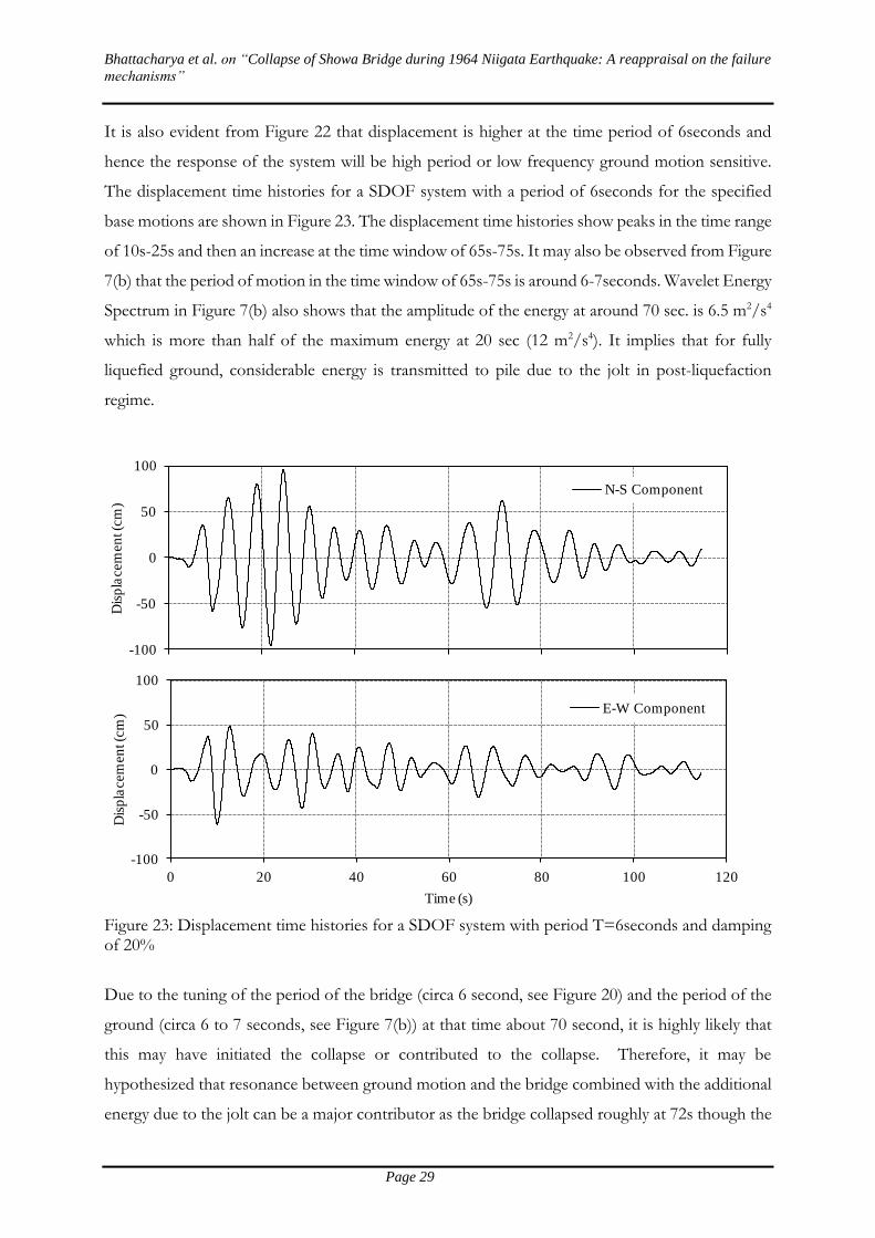
It is also evident from Figure 22 that displacement is higher at the time period of 6seconds and

hence the response of the system will be high period or low frequency ground motion sensitive.

The displacement time histories for a SDOF system with a period of 6seconds for the specified

base motions are shown in Figure 23. The displacement time histories show peaks in the time range

of 10s-25s and then an increase at the time window of 65s-75s. It may also be observed from Figure

7(b) that the period of motion in the time window of 65s-75s is around 6-7seconds. Wavelet Energy

Spectrum in Figure 7(b) also shows that the amplitude of the energy at around 70 sec. is 6.5 m2/s4

which is more than half of the maximum energy at 20 sec (12 m2/s4). It implies that for fully

liquefied ground, considerable energy is transmitted to pile due to the jolt in post-liquefaction

regime.

Figure 23: Displacement time histories for a SDOF system with period T=6seconds and damping of 20%

Due to the tuning of the period of the bridge (circa 6 second, see Figure 20) and the period of the

ground (circa 6 to 7 seconds, see Figure 7(b)) at that time about 70 second, it is highly likely that

this may have initiated the collapse or contributed to the collapse. Therefore, it may be

hypothesized that resonance between ground motion and the bridge combined with the additional

energy due to the jolt can be a major contributor as the bridge collapsed roughly at 72s though the

-100

-50

0

50

100

0 20 40 60 80 100 120

Dis

pla

cem

en

t (c

m)

Time (s)

E-W Component

-100

-50

0

50

100

Dis

pla

cem

en

t (c

m)

N-S Component


mechanisms”

ground displacement was larger at initial 10-25s. Haldar et al. (2008) also investigated the failure of

the Showa Bridge and they concluded that the soil of the riverbed under the bridge liquefied

sequentially and hence the flexibility of the soil-pile system increased with time. Yoshida et al. (2007)

and Kerciku et al. (2007, 2008) were also of the same opinion.

DISCUSSION

The role of in-depth analysis of case histories cannot be underestimated. Collapse of Showa Bridge

provides a unique insight into various failure mechanisms that needs to be checked for any bridge.

Three broad failure mechanisms for Showa Bridge piles can be postulated:

1. Bending failure due to inertia in the first part of the strong motion. This can be discarded

as the bridge did not fail in the initial 10 seconds..

2. Bending failure due to lateral spreading: This failure mechanism can be discarded as lateral

spreading started at about 83 seconds after the bridge collapsed. Also the piles close to the

bridge abutments did not fail where the lateral spreading was known to be severe. On the

contrary, the piles in the middle of the bridge failed where the lateral spreading is expected

to be the least.

3. The proposed mechanism is the tuning of the bridge with the ground during the jolt causing

large displacement at the pile which may have unseated the deck. It may also be mentioned

that the depth of the liquefied layer is more towards the left half of the bridge as is evident

from the liquefaction profile shown in Figure 6. Depending on the thickness of the

liquefied soil layer, the flexibility of the soil-pile system is more towards the left half of the

bridge and hence possibility of greater pile head deflection due to resonance. Therefore,

depending on the thickness of the liquefied layer and resulting resonance (tuning with the

earthquake), the deflections at the pile head is more on the left half of the bridge and is

adequate to unseat the bridge deck. This could explain the reason why collapse was mainly

observed on the left half of the bridge.

4. The current codes of practice or design guidelines does not consider all the above failure

mechanisms. It is therefore necessary to carry out seismic requalification studies of bridges

in liquefiable areas. A method to carry our seismic requalification studies is given by Sarkar

et al (2014)

5.0 CONCLUSION

Quantitative back-analysis has been carried out to understand the failure mechanism of Showa

Bridge. Following major conclusions may be summarised from the present study:


mechanisms”

1. Due to liquefaction induced soil stiffness degradation, time period of the middle of the

bridge (pile-soil-pier-deck system) increased from about 2seconds to about 6seconds. This

resulting high period of the bridge falls in the displacement sensitive zone of the response

spectra. Also the natural period of the liquefied soil falls in the range of 6- 7seconds in the

time window of 65s-75s leading to resonance between the ground motion and the bridge.

This resonance coupled with the jolt at 70 seconds of the earthquake is thought to be a

major contributor of failure of Showa Bridge.

2. Soil liquefaction profile as estimated by Hamada and O’Rourke (1992) shows more depth

of liquefaction on left half of the bridge. Depending on the thickness of the liquefied soil

layer and the corresponding period lengthening of the soil-pile system more tuning with

the earthquake (i.e. resonance) and enhanced pile head deflection is expected on the left

half side of the bridge. This may explain the observation that collapse occurred only on the

left half of the bridge.


mechanisms”

3. REFERENCES:

1. Abe, K. (1975). Re-examination of the fault model for the Niigata earthquake of 1964. Journal

of Physics of the Earth, 23, 349-366

2. Adhikari S and Bhattacharya S (2008) Dynamic instability of pile-supported structures in

liquefiable soils during earthquakes, Shock and Vibration, Vol 16(6), pp 665-685

3. Anon. (1966), Brief explanation on pictures taken at the moment of Niigata Earthquake, Soils

and Foundations, VI (1), pp i-vi.

4. API (2003): American Petroleum Institute, Recommended Practice for planning designing and

constructing fixed offshore platforms.

5. Berrill J, Yasuda S (2002) Liquefaction and piled foundations: Some issues. Journal of

Earthquake Engineering, 6, Special Issue 1:1-41

6. Bhattacharya S (2003) Pile Instability during Earthquake Liquefaction. PhD thesis, University

of Cambridge, UK

7. Bhattacharya S, Bolton MD, Madabhushi SP (2005) A reconsideration of the safety of piled

foundations in liquefied soils. Soils and Foundation, 45(4): 13-24.

8. Bhattacharya S, Blakeborough A, Dash SR (2008) Learning from collapse of piles in liquefiable

soils. Proc., Institution of Civil Engineering, Special Issue of Civil Engineering, 161: 54-60

9. Bhattacharya S, Dash SR, Adhikari S. (2008) On the mechanics of failure of pile-supported

structures in liquefiable deposits during earthquakes'. CURRENT SCIENCE, 94 (5), pp 605-

611.

10. Bhattacharya S, Madabhushi SPG (2008) A critical review of methods for pile design in

seismically liquefiable soils. Bull Earthquake Eng, 6: 407-446

11. Bhattacharya S, Adhikari S, Alexander NA (2009) A simplified method for unified buckling

and free vibration analysis of pile-supported structures in seismically liquefiable soils. Soil

Dynamics and Earthquake Engineering, 29: 1220-1235

12. Bhattacharya S. and Goda, K (2013) Probabilistic buckling analysis of axially loaded piles in

liquefiable soils. Soil Dynamics and Earthquake Engineering, 45:13-24

13. Bhattacharya, S and Tokimatsu, K (2013): Collapse of Showa Bridge revisited, International

Journal of Geoengineering Case Histories, 3 (1). 24 - 35. ISSN 1790-2045

14. Brandenberg SJ (2005) Behaviour of pile foundations in liquefied and laterally spreading

ground. Ph.D. thesis, University of California at Davis, California, USA

15. Davis, R. O., and Berrill, J. B., (2001). Liquefaction at the Imperial Valley Wildlife Site. Bulletin

of the New Zealand Society for Earthquake Engineering, 34(2): 91-106.


mechanisms”

16. Dash SR, Bhattacharya S, Blakeborough A (2010) Bending-buckling interaction as a failure

mechanism of piles in liquefiable soils. Soil Dynamics and Earthquake Engineering, 30:32-39

17. Elgamal, A., Zeghal, M. and Parra, E., (1996) Liquefaction of reclaimed island in Kobe, Japan.

Journal of Geotechnical and Geoenvironmental Engineering, ASCE, 122(1): 39-49.

18. Elgamal A, Lu J, Yang Z, and Shantz T (2009) Scenario-focused three-dimensional

computational modeling in geomechanics. Proc., 4th International Young Geotechnical

Engineers' Conference, ISSMGE, Alexandria, Egypt, (Invited Keynote Lecture Paper).

19. Finn WDL, and Fujita N (2002) Piles in liquefiable soils: seismic analysis and design issues. Soil

Dynamics and Earthquake Engineering, 22:731-742

20. Fukuoka M (1966). Damage to Civil Engineering Structures. Soils and Foundations, 6 (2):45-

52

21. Goda, K., and Atkinson, G.M. (2010). Intraevent spatial correlation of ground-motion

parameters using SK-net data. Bulletin of the Seismological Society of America, 100, 3055-

3067.

22. Goda, K. (2011). Interevent variability of spatial correlation of peak ground motions and

response spectra. Bulletin of the Seismological Society of America, 101, 2522-2531.

23. Halder S, Sivakumarbabu GL, Bhattacharya S (2008) Bending and buckling Buckling and

bending response of slender piles in liquefiable soils during earthquakes. Geomechanics and

Geoengineering: An International Journal, 3(2): 129-143

24. Hamada M (1992) Large ground deformations and their effects on lifelines: 1964 Niigata

earthquake. Case Studies of liquefaction and lifelines performance during past earthquake.

Technical Report NCEER-92-0001, Japanese case studies, National Centre for Earthquake

Engineering Research, Buffalo, NY

25. Hamada M, O’Rourke TD (1992) Case studies of liquefaction and lifeline performance during

past earthquakes. Japanese case studies, Technical Report NCEER-92-0001.

26. Horii K (1968) General report on the Niigata earthquake. Tokyo Electrical Engineering College

Press. Part 3: Highway Bridges, 431-450.

27. Hurukawa, N., and Harada, T. (2013). Fault plane of the 1964 Niigata earthquake, Japan,

derived from relocation of the mainshock and aftershocks by using the modified joint

hypocenter determination and grid search methods. Earth Planets Space, 65, 1441-1447.

28. Idriss, I.M., and Boulanger, R.W. (2008) Soil Liquefaction During Earthquakes, Earthquake

Engineering Research Institute, Oakland, CA, 235 pp.

29. Ishihara K (1993) Liquefaction and flow failure during earthquakes. Geotechnique, 43 (3):351-

415


mechanisms”

30. Iwasaki T (1984) A case history of bridge performance during earthquakes in Japan. Keynote

lecture at the International Conference on Case histories in Geotechnical Engineering, May 6-

11, University of Missouri – Rolla, Shamsher Prakash (eds)

31. Iwasaki T (1986) Soil liquefaction studies in Japan. State-of-the-art, Technical Memorandum

No. 2239, Public Works Research Institute, Tsukuba, Japan.

32. JSA (2004) JIS A 5525 Steel pile pipe. Japanese Standard Association, Japan

33. Kazama M, Sento N, Uzuoka R, Ishihara M (2008) Progressive damage simulation of

foundation pile of the Showa Bridge caused by lateral spreading during 1964 Niigata

Earthquake. Geotechnical Engineering for Disaster Mitigation and Rehabilitation, 171-176

34. Kerciku A A, Bhattacharya S, Burd HJ, Lubkowski ZA (2008) Failure of Showa Bridge during

1964 Niigata earthquake: Lateral spreading or buckling instability? Proc., 14th World

Conference on Earthquake Engineering, Beijing, China.

35. Kerciku AA, Bhattacharya S, Burd H J (2007) Why do pile supported bridge foundations and

not abutments collapse in liquefiable soils during earthquakes? Proceedings of the 2nd Japan

Greece Workshop on seismic design, observation and retrofit of foundations. Japanese Society

of civil engineers: 440-452.

36. Kokusho T, Hara T, Hiraoka R (2004) Undrained shear strength of granular soils with different

particle gradations. Journal of Geotechnical and Geoenvironmental Engineering, ASCE,

130(6): 621-629

37. Kramer SL (1996) Geotechnical earthquake engineering. Prentice-Hall, Civil Engineering and

Engineering Mechanics Series

38. Kudo K, Uetake T, Kanno T (2000) Re-evaluation of nonlinear site response during the 1964

Niigata earthquake using the strong motion records at Kawagishi-cho, Niigata City. Proc., 12th

World Conference on Earthquake Engineering, Auckland, New Zealand

39. Lombardi D and Bhattacharya, S (2013) Modal analysis of pile-supported structures during

seismic liquefaction. Earthquake Engineering and Structural Dynamics, doi: 10.1002/eqe.2336

40. Maheshwari BK, Sarkar R (2011) Seismic Behaviour of Soil-Pile-Structure Interaction in

Liquefiable Soils: A Parametric Study. International Journal of Geomechanics, ASCE, 11

(4):335-347

41. Meyerhof GG (1957) Discussion on soil properties and their measurement. Proc., 4th

International Conference on Soil Mechanics and Foundation Engineering.

42. Nobuyuki Morikawa, N., Kanno, T., Narita, A., Fujiwara, H., Okumura, T., Fukushima, Y.,

and Guerpinar, A. (2008). Strong motion uncertainty determined from observed records by

dense network in Japan. Journal of Seismology, 12, 529-546.


mechanisms”

43. Rollins KM, Gerber TM, Lane JD, Ashford, SA (2005) Lateral resistance of a full-scale pile

group in liquefied sand. Journal of Geotechnical and Geoenvironmental Engineering, ASCE,

131:115–125

44. SAP 2000: V10.1. Integrated Software for Structural Analysis and Design, Computer and

Structures Inc (CSI), Berkeley, California, USA, August 2004.

45. Shiba, Y., and Uetake, T. (2011). Rupture process of the 1964 MJMA 7.5 Niigata earthquake

estimated from regional strong-motion records. Bulletin of the Seismological Society of

America, 101, 1871-1884.

46. Sarkar R, Maheshwari BK (2012) Effects of Separation on the Behaviour of Soil-Pile

Interaction in Liquefiable Soils. International Journal of Geomechanics, ASCE, 12 (1): 1-13

47. Sarkar, S, Bhattacharya S and Maheswari, B.K (2014): Seismic Requalification of Piled

Foundations in Liquefiable Soils, Indian Geotechnical Journal (to appear)

48. Shamoto Y, Zhang JM, Goto S (1997) Mechanism of large post-liquefaction deformation in

saturated sand. Soils and Foundations, 37(2):71-80

49. Takata T, Tada Y, Toshida I, Kuribayashi E (1965) Damage to bridges in Niigata earthquake.

Report no. 125-5, Public Works Research Institute (in Japanese)

50. Tokimatsu K., Suzuki H., and Sato M., (2005) Effects of Inertial and kinematic interaction on

seiasmic behaviour of pile with embedded foundation. Soil Dynamics and Earthquake

Engineering, 25: 753-762.

51. Towhata I (1999) Photographs and Motion Picture of the Niigata City Immediately after the

1964 earthquake. Japanese Geotechnical Society (CD-Rom)

52. Towhata I., Sasaki Y., Tokida K., Matsumoto H., Tamari Y., Yamada K., (1992) Prediction of

Permanent Displacement of Liquefied Ground by Means of Minimum Energy Principle. Soils

and Foundations, 32 (3): 97-116.

53. Vaid YP, Thomas J (1995) Liquefaction and post liquefaction behavior of sand. Journal of

Geotechnical Engineering, ASCE, 121(2):163–173

54. Yasuda S, Yoshida N, Kiku H, Adachi K, Gose S (1999) A simplified method to evaluate

liquefaction-induced deformation. Proc. Earthquake Geotechnical Engineering, Balkema,

Rotterdam, 2:555-566

55. Yoshida N, Tazoh T, Wakamatsu K, Yasuda S, Towahata I, Nakazawa H, Kiku H (2007)

Causes of Showa Bridge collapse in the 1964 Niigata earthquake based on eyewitness testimony.

Soils and Foundations, 47(6): 1075-1087

56. Yoshimi Y (2003) The 1964 Niigata Earthquake in retrospect. Soft Ground Engineering in

Coastal Areas, Taylor & Francis, 53-59


mechanisms”

57. Zeghal M., and Elgamal A., (1994) Analysis of Site Liquefaction Using Earthquake Records,

Journal of Geotechnical Engineering, ASCE, 120(6): 996-1017.

58. Zhou Z, Adeli H (2003a) Time-Frequency Signal Analysis of Earthquake Records Using

Mexican Hat Wavelets. Computer-Aided Civil and Infrastructure Engineering, 18: 379–389

59. Zhou Z, Adeli H (2003b) Wavelet Energy Spectrum for Time-Frequency Localization of

Earthquake Energy. International Journal of Imaging Systems and Technology, 13(2), 133-140.

60. Zhao, J.X., Zhang, J., Asano, A., Ohno, Y., Oouchi, T., Takahashi, T., Ogawa, H., Irikura, K.,

Thio, H.K., Somerville, P.G., Fukushima, Y., and Fukushima, Y. (2006). Attenuation relations

of strong ground motion in Japan using site classification based on predominant period.

Bulletin of the Seismological Society of America,96, 898-913.

collapse of showa bridge during 1964 niigata earthquake… · bhattacharya et al. on “collapse of...

Documents