COINTEGRA TION AND UNIT ROOTS Juan J. Dolado Bank of Spain

Tim J enkinson Keble College, University of Oxford and CEPR

Simon Sosvilla-Rivero University of Birmingham

Abstract. This paper provides an updated survey of a burgeoning literature on testing, estimation and model speciftcation in the presence of integrated variables. Integrated variables are a speciftc class of non-stationary variables which seem to characterise faithfully the properties of many macroeconomic time series. The analysis of cointegration develops out of the existence of unit roots and offers a generic route to test the validity of the equilibrium predictions of economic theories. Special emphasis is put on the empirical researcher's point of view.

Keywords. Unit root, cointegration, trends, error correction mechanisms.

1. Introduction

Economic theory generaHy deals with equilibrium relationships. Most empirical econometric studies are an attempt to evaluate such relationships by summarising economic time series using statistical analysis. To apply standard inference procedures in a dynamic time series model we need the various variables to be stationary, since the majority of econometric theory is built upon the assumption of stationarity. Until recently, this assumption was rarely questioned, and econometric analysis proceeded as if aH the economic time series were stationary, at least around sorne deterministic trend function which could be appropriately removed. However, stationary series should at least have constant unconditional mean and variance over time, a condition which appears rarely to be satisfied in economics. The importance of the stationarity assumption had been recognised for many years, but the important papers by Granger and Newbold (1974), Nelson and Kang (1981) and Nelson and Plosser (1982) alerted many to the econometric implications of non-stationarity. Integrated variables are a specific class of non-stationary variables with important economic and statistical properties. These are derived from the presence of unit roots which give rise to stochastic trends, as opposed to pure deterministic trends, with innovations to an integrated process being permanent

0950-0804/90/03 0249-25 $02.50/0 © 1990 J. J. Dolado, T. Jenkinson and S. Sosvilla-Rivero JOURNAL OF ECONOM1C SURVEYS Vol. 4, No. 3

1

-" -250 DOLADO, JENKINSON AND SOSVILLA-RIVERO

~nstead of transient. For example, the presence of a large permanent component m aggregate output conflicts with traditional formulations of both Keynesian and Classical macroeconomic theories in terms of countercyclical policies, implying, in addition, that the welfare costs and benefits of policy actions are far different than when output movements are seen as transitory deviations from a slowly growing natural leve!.

The presence of, at least, a unit root is implied by many economic models by the rational use of available information by economic agents. Standard applications inelude futures contracts, stock prices, yield curves, real interest rates, exchange rates, money velocity, hysteresis theories of unemployment, and, perhaps the most popular, the implications of the permanent in come hypothesis for real consumption.

Statisticians have been aware for many years of the existence of integrated series and, in fact, Box and Jenkins (1970) argue that a non-stationary series can be transformed into a stationary one by successive differencing of the series. Therefore, from their point of view, the differencing operation seemed to be a pre-requisite for econometric modelling both from an univariate and a multivariate perspective. However Sargan (1964), Hendry and Mizon (1978) and Davidson et al. (1978), among others, have criticised on a number of grounds the specification of dynamic models in terms of differenced variables only, especially because it is then impossible to infer the long-run steady state solution from the estimated mode!.

Granger (1983) and Granger and Weiss (1983), resting upon the previous ideas point out that a vector of variables, all of which achieve stationarity afte; differencing, may have linear combinations which are stationary without differencing. Engle and Granger (1987) formalise the idea of variables sharing an equilibrium relationship in terms of cointegration between time series, providing us with tests and an estimation procedure to evaluate the existence of equilibrium relationships, as implied by economic theory, within a dynamic specification framework. Standard examples inelude the relationship between real wages and productivity, nominal exchange rates and relative prices, consumption and disposable income, long and short-term interest rates, money velocity and interest rates, production and sales, etc.

In view of this epidemic of martingales in economics, a voluminous literature on testing, estimation, prediction, control and model specification in the presence of integrated variables has developed in the last few years. 1 The purpose of this survey is to provide a useful guide through this increasingly technical literature, paying special attention to the point of view of the applied researcher with a good grounding in econometrics, who being a non-specialist in this particular subject wants to get a unified coverage of the main techniques available in this field.

The paper is organised as follows. The concepts of cointegration and unit roots are introduced in Section 2. In Section 3 we survey several alternative tests for the existence of unit roots, ineluding cases where seasonality is present. Section 4 deals with alternative definitions of integration. Section 5 examines

SWkA'110NAND UNIT RÓOTS 251

the applicatiotl ~j~me of the previous tests to determine the existence of cointegrating relationships. Section 6 contains a review of some new test procedures for cointegration. Finally, brief conelusions follow in Section 7.

2. Unit roots and cointegration Wold's (1938) decomposition theorem states that a stationary time series process with no deterministic component has an infinite moving average (MA) representation. This, in turn, can be represented approximately by a finite autoregressive moving average (ARMA) process (see, e.g. Hannan, 1970).

However, as was mentioned in the Introduction, some time series need to be appropriately differenced in order to achieve stationarity. From this comes the ~efi~ition of ~ntegration (as adopted by Engle and Granger, 1987): A variable Yt IS sald to be mtegrated of order d [or Yt - I(d)] if it has stationary, invertible non-deterministic ARMA representation after differencing d times. Thus, a tim~ series integrated of order zero is stationary in levels, while for a time series integrated of order one, the first difference is stationary. A white noise series and a s~able first-order autoregressive [AR(I)] process are examples of 1(0) series, whIle a random walk process is an example of an 1(1) series.

Granger (1986) and Engle and Granger (1987) discuss the main differences between pro ces ses that are 1(0) and 1(1). They point out that an 1(0) series: (i) has finite variance which does not depend on time, (ii) has only a limited memory of its. past be~.~viour (i.e. the effects of a particular random innovation are only transttory), (m) tends to fluctuate around the mean (which may inelude a ~eterministic trend), and (iv) has autocorrelations that deeline rapidly as the lag mcreases. For the case of an 1(1) series, the main features are: (i) the variance depends. upo.n time and goes to infinity as time goes to infinity, (ii) the process has an mfimtely long memory (i.e. an innovation will permanently affect the process), (iii) it wanders widely, and (iv) the autocorrelations tend to one in magnitude for all time separations.

Consider now two time series Yt and Xt which are both I(d) (i.e. they have c~mpatible long-run properties). In general, any linear combination of Yt and Xt

wl11 be also I(d). If, however, there exists a vector (1, -(3)', such that the combination

Zt = Yt - ex - (3Xt (1)

is I(d - b), b > O, then Engle and Granger (1987) define Yt and Xt as cointegrated of arder (d, b) [or (Yt, Xt)' - CI( d, b)], with (1, - (3)' called the cointegrating vector. Note that a constant term has been included in (1) in order to allow for the possibility that Zt may have a non-zero mean.

The concept of cointegration tries to mimic the existence of a long-run equilibrium to which an economic system converges over time. If, e.g., economic theory suggests the following long-run relationship between Yt and Xt

Yt = ex + (3Xt (2)

2

DOLADO, JENKINSON AND SOSVILLA-RIVERO

then Zt can be interpreted as the equilibrium error (i.e., the distance that the system is away from the equilibrium at any point in time).

Engle and Granger also show that if Yt and Xt are cointegrated C/(I, 1), then there must exist an error correction model (ECM) representation of the following form 2

(3)

where .:l denotes the first-order time difference (i.e . .:lYt = Yt - Yt-I) and where {e¡) is a sequence of independent and identically distributed random variables with mean zero and variance CT~ (i.e. et - iid(O, CT~». Furthermore, they prove the converse result that an ECM generates cointegrated series.

Note that the term Zt-I in equation (3) represents the extent of the disequilibrium between levels of y and x in the previous periodo The ECM states that changes in Yt depend not only on changes in Xt, but al so on the extent of disequilibrium between the levels of y and x. The appeal of the ECM formulation is that it combines flexibility in dynamic specification with desirable long-run properties: it could be seen as capturing the dynamics of the system whilst incorporating the equilibrium suggested by economic theory (see Hendry and Richard, 1983).3

Based upon the concept of cointegration (and on its closely related concept of ECM representation), Engle and Granger suggest a 2-step estimation procedure for dynamic modelling which has become very popular in applied research. Let us assume that Yt and Xt are both 1(1), then the procedure goes as follows:

(i) First, in order lO test whether the series are cointegrated, the 'cointegrating regression'

Yt = ex + (3Xt + Zt (4)

is estimated by ordinary least squares (OLS) and it is tested whether the 'cointegrating residuals' Zt = Yt - eX - SXt are 1(0). Stock (1987) has shown that if two 1(1) series are cointegrated, then the OLS estimates from equation (4) provide 'super-consistent' estimates of the cointegrating vector, in the sense that they converge to the true parameter at arate proportional to the inverse sample size, T- I, rather than at T- 1I2 as in the ordinary stationary case. 4 The intuition behind this remarkable result can be seen by analysing the behaviour of the OLS estimator of (3 in (4) (where the constant is eliminated for simplicity), when Zt - iid(O, CT~) and Xt follows a random walk:

.:lXt = et; (xo = O, et - iid(O, CT~»

Integrating (5) backwards we get t

Xt = 2:: e; = St ;=1

(5)

and therefore var(xr) = tCT~, exploding as Tt oo. 5 Nevertheless T- 2ExT

converges to a random variable. Similarly the cross-moment T-1I2ExtZt will

rotNrEGRATION AND UNIl' ROOTS 2S~

explode, in contrast to the stationary case, where it is asymPtoticall~ normally distributed. In the 1(1) case T-1ExtZt converges also to a random vanable. Both random variables are functionals of Brownian Motions or Wiener processes, which will be denoted henceforth, in general, as I(W) (see Phillips (1987), Phillips and Perron (1988) and Park and Phillips (1988) for a general discussion on convergence of the aboye mentioned distributional limits). From the expression for the OLS estimator of (3 we obtain

S - (3 = EXtZt/ExT

it follows from the previous discussion that T(S - (3) is asymptotically the ratio of two non-degenerate random variables, and it is in general not normal. Thus, standard inference cannot be applied to S, even if it is 'super-consistent', a question to which we will come back in Section 6.

(ii) Finally, the residuals Zt are entered into the ECM. Now, all the variables in equation (3) are 1(0) and conventional modelling strategies can be applied.

3. Testing the order of integration of the relevant variables Once the relevant set of variables suggested by economic theory has been identified, the first stage in testing for cointegration between those variables is to determine the order of integration of the individual time series.

Several statistical tests for unit roots have been developed to test for stationarity in time series. Since many macroeconomic series have been found to be integrated of order one (see, e.g. Nelson and Plosser, 1982), we will only consider tests for a single unit root.

The previous tests can also be applied, with a slight change in their interpretation, for sequential testing of unit roots, i.e. when one wants to compare a null hypothesis of k unit roots with an alternative of k - 1 unit roots. In the sequential procedure, the investigator should start with the largest k under consideration and work down; that is, decrease d by one each time the null hypothesis is rejected. 6

3.1. Tests 01 unit roots

(i) Dickey and Fuller (1979, 1981) present a class of test statistics, known as Dickey-Fuller (DF) statistics, generally used to test that apure AR(1) process (with or without drift) has a unit root.

Let the time series Yt satisfy the following data generating pro ces s (DGP)

Yt = (30 + (3¡( + PYt-1 + et (6)

where et - iid(O, CT~), t is a time trend and the initial condition, Yo, is assumed to be a known constant (zero, without loss of generality). Equation (6) can al so be written as

t t t Yt = (30 2:: p t-) + (31 2:: jp t -) + 2:: e}pt-} (7)

}=I }=I }=I

3

254 DOLADO, JENKINSÓN AND SOSVILLA-RIVERO

while in the case that P = 1

Yt = (3ot + (3¡(t + 1)/2 + St (8)

where St = ~5=1 ej

Dickey and Fuller (1979) consider the problem of testing the null hypothesis Ho: p = 1 versus H I: P < 1, i.e. non-stationarity vs. stationarity around a deterministic trend, suggesting OLS estimation of a reparameterised version of (6), i.e.

LlYt = (30 + (3lt + ')'Yt-I + et (9)

where Ho: p = 1 is equivalent to Ho: ')' = O (since ')' = p - 1). The test is implemented though the usual t-statistic of ..y, denoted here as T7 • In addition, Dickey and Fuller (1981) suggest two F-statistics for the joint null hypothesis (30 = (31 = ')' = O and (31 = ')' = O, denoted as <P2 and <P3 respectively. Note that under the null hypothesis Tn <P2 and <P3 will not have the standard t and F distributions, instead they are functions of Brownian motion; we must use the asymptotic distributions tabulated in Fuller (1976, p. 373) and in Dickey and Fuller (1981, p. 1,063) respectively. If (31 = O «(30 = O) in (9), the t and Fstatistics, corresponding to Ho: ')' = O and H I: (30 = ')' = O, are denoted T,,(T) and <PI respectively and the corresponding critical values are also given in the previous references. In all cases the critical values given there crucially depend upon the sample size. It should al so be noted that the critical values depend upon the 'nuisance' parameters contained in the model and in the DGP. To discuss this more formally, consider the sample variance of Yt when it is generated by (8) (i.e. p = 1)

T-IEyl= T-IE [«(30 + (31/2)2t2 + «(31/2)2t4 + sl + «(30 + (31/2)(3¡(3 + 2«(30 + (31/2)tSt + (3lt 2St] (10)

From the distributional results in Park and Phillips (1988), it is known that T- 2ESl, T- 5/2EtSt and T- 712Et 2St tend to j(W), hence, by taking probability limits in (10), we get

T-IEYl~(3f!20 O(T4) + «(30 + (31/2)(31/4 O(T3) + (3j(W)O(T5/2)

+ «(30 + (31/2)2/3 O(T2) + 2«(30 + (31/2)j(W)O(T3/2) + j(W)O(T)

whereby it is seen that

T-5Eyl~(3T/20

T-3Eyl~(3ij¡3

T-2Eyl~ j(W)

if (31 -,é. O if (30 -,é. O, (31 = O if (30 = (31 = O

(11)

That is, if the unit root pro ces s contains a linear trend or a drift, its variability will be dominated by a quadratic or a linear trend which, appropriately normalised, converges to constants. It is only when (30 = (31 = O that it converges to a non-standard distribution. This means that for example, if (31 -,é. O in (8) and

COINTE€lItATlON AND UNIT ROOTS 255

the modd is estimated as in (9), the quadratic term in (10) will dominate the integrated process and normality of the T7 will follow. Similarly if (30 -,é. O in (8) (with (31 = O) and only a constant appears in (9), the linear trend will dominate and normality of T" will also follow. 7 It is only when (30 = (31 = O, both in the DGP and in the model, that the non-standard distribution will dominate. This implies that in order to use the DF critical values if a linear trend is included in the maintained hypothesis (9), the relevant null hypothesis should be a random walk with drift «(30 -,é. O), whilst if only a drift is included in (9), the relevant null hypothesis is a random walk without drift. 8

From the previous discussion we consider that the following testing strategy is most appropriate. First, start by the most unrestricted model (9), «(30 -,é. O, (31 -,é. O) if it is suspected that the differenced series has a drift. Then use T7 to test for the null hypothesis. If it is rejected there is no need to go further. If it is not rejected, test for the significance of the trend under the null. If it is significant, then test again for a unit root using the standardised normal. If the trend is not significant in the maintained model, estimate (9) without trend «(31 = O). Test again for the unit root using T". If the null hypothesis is rejected, again there is no need to go further. If it is not rejected, test for the significance of the constant under the null hypothesis and so on.

(ii) In the analysis of the DF tests, we have assumed that the DGP is apure AR(l) process. If instead, the DGPis AR(p)

let

p

Yt = (30 + (3¡( + ~ PiYt-i + et i=1

p

AP - ~ PiAP-i = O i=1

(12)

(13)

be the characteristic equation of the time series, where A(i = 1, ... , p) are the eigenvalues of the process. Dickey and Fuller (1979, 1981) consider the problem of testing the null hypothesis Ho: Al = 1 and 1 A21 < 1 for i = 2, ... , p, suggesting OLS estimation of the reparameterised regression model

P- I

LlYt = (30 + (3¡( + ')'IYt-1 + ~ ')'2iLlYt-i + et i=1

(14)

where p is large enough to ensure that the residual series et is white noise. The tests are based on the t-ratio on..yl and are known as 'Augmented Dickey Fuller' (ADF) statistics. The critical values are the same as those discussed for the DF statistics, since the ..y2i (i = 1, ... , p - 1) estimates converge to their true values at arate O(T- 1I2

), being asymptotically dominated by the distribution of "YI which, as we mentioned in (4), is O(T- I

). The same testing strategy discussed aboye, applies in this case. 9

The sample distribution of the ADF statistics critically depend on the assumption that the time series Yt is generated by apure AR process. However,

4

since there is evidence that many macroeconomic series contain moving average (MA) components (see Schwert, 1987), we would want to consider also the possibility of an MA component in the DGP, so that the mill hypothesis would be that the data are generated by a mixed autoregressive integrated moving average (ARIMA) process.

Said and Dickey (1984) extend the ADF test by exploiting the fact that an ARIMA (p, 1, q) process can be adequately approximated by a high-order autoregressive process, AR(I), where / = O(TII3

) as Ti oo. In practice the test proceeds as before with p in (12) and (14) equal to /. This approach permits one to test the null hypothesis of the presence of a unit root without knowing the orders of p and q. However, it involves the estimation of additional nuisance parameters which reduces the effective number of observations due to the need for extra initial conditions.

When p and Q. are known, Said and Dickey (1985) present a test for the hypothesis that the process is ARIMA (p, 1, q), Le.

Ho: cP(L)~Yt = O(L)et

where cP(.) and 0(.) are pth and qth order polynomials in the lag operator L, versus the alternative hypothesis that it is ARIMA (p, O, q)

HI: cP(L)(l - pL)Yt = O(L)et

To perform the test of p = 1, we specify initial estimates of the parameters that are consistent under the null and alternative hypothesis. We next perform a one-step of the Gauss-Newton numerical estimation procedure (see, e.g., Harvey, 1981 p. 17). The t-statistic associated with p, after applying the iteration has the

. limiting distribution of 7, tabulated by Fuller (1976, p. 373). Similarly if the series mean y is subtracted from each observation of Yt prior to analysis, the t-statistic has the limiting distribution of 7".

(iii) An alternative approach, based upon the DF procedure has been presented by Phillips (1987) and Phillips and Perron (1988). While the ADF statistics are based upon the assumption that the disturbance term et is identically and independently distributed, they suggest amending these statistics to allow for weak dependence and heterogeneity in et. Under such general conditions, a wide class of DGP's for et, such as most finite order ARIMA (p, 0, q) models, can be allowed. The procedure consists of computing the DF statistics and then using sorne non-parametric adjustment of 7" and 7 7 in order to eliminate the dependence of their limiting distributions on additional nuisance parameters stemming from the ARIMA process followed by the error terms. Their adjusted counterparts are denoted Z(7,,) and Z(77 ), respectively.

For the regression model (9), with (31 = O, Phillips and Perron (PP) define

[

T ] -112 Z(7,,) = (S/STm)7,,-0.5(S}m-S2)T S}m ~ (Yt-y_¡)2 (15)

where T is the sample size and m is the number of estimated autocorrelations;

"COINTEORATlGN¡AND UNI1"ROOTlS 257

Y_I = (T- l)-Ib ! Yt_l,S2 and 7" are, respectively, the sample variance of the residual s and the t-statistic associated with 'Y from the regression (9) (with (31 = O); and S}m is the long-run variance estimated as lO

T I T

S}m = T- I ~ el + 2T- 1 ~ W sm ~ etet-s (16) t=1 s=1 t=s+1

where e are the residuals from the regression (9) and where the triangular kernel

Wsm = [1 - s(m + 1)], s = 1, ... , m (17)

is used to ensure that the estimate of the variance S}m is positive (see Newey and West, 1987)

When (31 .,t. O in (9), the corresponding statistic is

Z(77 ) = (§/Srm)77 - (§}m - §2)T3 {4Srm [3Dxx] 1121- 1 (18)

where § and §Tm are defined as aboye, but with the residual e obtained from the estimation of (9) with (31 .,t. O. Dxx is the determinant of the regressor cross-product matrix, given by

Dxx = [T2(T2 - l)fl2] EY~-1 - T(EtYt- ¡)2 + T(T + 1)EtYt-1EYt-l - [T(T + 1)(2T + 1)/6] (EYt- ¡)2

The Phillips and Perron statistics have the same limiting distributions as the corresponding DF and ADF statistics, provided that mi 00 as Ti 00, such that m/TI14 iO.

(iv) Simulation evidence in Molinas (1986) and Schwert (1986, 1989), shows that the tests proposed by Dickey and Fuller and by Phillips and Perron are affected by the process generating the data in large finite samples. In particular, when the underlying process is ARIMA (0,1,1) with a MA parameter close to one, the ADF and PP statistics have critical values that are far below the Dickey-Fuller distributions (Le. these tests will lead to the conclusion that economic data are stationary too frequently). The intuition behind this result is that if the DGP of Yt is

~Yt = (1 - OL)et (19)

if O is close to one, (1 - L) will tend to cancel on both sides of (19), giving the impression that Yt behaves like a white noise. However, the Said and Dickey (1984) high-order autoregressive t test for the unit root, with a suitable choice of /, has size close to its nominal level for all values of the MA parameter. Schwert suggests searching for the correct specification of the ARIMA process before testing for the presence of a unit root in the AR polynomial and provides the relevant critical values for the Said and Dickey (1984), Phillips (1987) and Phillips and Perron (1988) tests based on Monte Carlo experiments.

(v) Hall (1989) proposes a new approach to testing for a unit root in a time series with a moving average component based on an instrumental variable (IV) estimator

5

DOLADO, JEJ'ltKINsON ANO SOSVIL'LA-RIVERO

Let Yt be generated by the DGP

Yt = #0 + #It + PYt-1 + (J(L)ct (20)

where (J(L) is again a q-th order lag polynomial. Then, the IV estimator for model (20) is defined as follows

- - - IV' I

( )-I(T) [#0, #1, p¡] = ~ ZItXIt ~ ZItYt (21)

where ZIt=(I,t,Yt-k) and X It =(1,t,Yt-¡), k=(q+ 1) (see Dolado (1989) for the choice of optimal IV in this framework). For the model (20) when #1 = O, the IV estimator is given by

[#0, ¡h] IV' = (~ Z2tXiJ 1 (~ Z2tyr) (22)

where now Z2t=(I,Yt-d,XIt =(1,Yt-¡) Let l(¡j IV) and i(Plv ) be the t-statistics associated with the null hypothesis

P = 1 in (19) (with and without trend), then Hall proves that

- -(;: IV)/ -Trv = Se7 \jJI S=? 7 7 (23) and

A A{';, IV)/ A Trv = Set\jJ2 S=?7p. (24)

where S~, §2 and §2 are consistent estimators of the variances of c and the long-run variance e(=(J(L)c) obtained as in (16) and (17).

(vi) As it might have been noticed, one important limitation of aH of the previous testing procedures is that they are not independent of the nuisance parameters contained in the deterministic component of the time-series process. This limitation has produced an alternative strand in the literature on testing. In this respect, Bhargava (1986) has developed most powerful invariant (MPI) tests for the null hypothesis corresponding to DGP (9) (with and without trend). These tests are valid in smaH samples and are independent of the nuisance parameters, but only valid for the AR(1) case. They are based upon trans-formations of Von Neumann type ratios, as for example the Durbin-Watson approach emphasised by Sargan and Bhargava (1983) in a different context, as discussed below. The statistics proposed to test Ho: P = 1, when #1 = O and #1 -:¡t. O, are given by

(25)

and

(26)

. ·''<i:OINTEGRA TlON ANDUNIT ROOTS 259

wher.e D = (T - 1)-2 ¿; {[(T - I)Yt - (t - I)YT - (T - t)YI - (T - 1)(y - 0.5(YI + YT »] 2

The corresponding critical values are given by Bhargava (1986, p. 378). The test is found to have slightIy greater power than the tests proposed by Dickey and Fuller, when the data are generated by an AR(1) process.

(vii) Another limitation of all the previous testing procedures is that the distributions of the corresponding statistics are non-standard and hence a different set of critical values has to be used in each case. This problem has originated a new strand of research (see Phillips and Ouliaris, 1988), which exploits the fact that differencing a stationary series induces a unit root in the moving average representation. This fact pfovides a diagnostic for testing whether the series is 1(0) or 1(1), by using the long-run variance of the first difference of the time series Yt. To clarify the interpretation of the test, let us assume that Yt is generated by

Then the long-run variance of ~Yt is a2 = (T~ (1) 2. If (JI -:¡t. 1 and (J '(1) -:¡t. O, then a2 is finite, whilst if (J¡ = 1, a2 is zero. In other words, if the time series Yt is 1(0), ~Yt will have a2 = O, whereas if it is 1(1), (T2 -:¡t. O. Therefore the null hypothesis is Ho: a 2 -:¡t. O or Ho: 7

2 = a2/a~ -:¡t. O, getting rid of the units of measurement. Obtaining an estimate of a 2 as in (16), Phillips and Ouliaris prove that

(27)

Since only the alternative hypothesis is a simple hypothesis, i.e. H¡: 7 2 = O, Phillips and' Ouliaris propose a bounds procedure based upon the corresponding confidence interval in (27), yielding

(28)

where z", is the (1 - a) percentage point of the standard normal distribution. According to the bounds test, Ho is rejected if the upper limit of 7

2 in (28) is sufficiently small. Similarly Ho is not rejected if the lower bound is sufficientIy large. Phillips and Ouliaris recommend using 0.10 as the rejection point for the upper and lower bound. Simulation results show, however, that the suggested value can be very conservative in sorne instances. For example if the DGP is ARIMA (1, 1, 1) with parameter values in the interval ( - 0.6,0.6), the average upper bound is 0.45 whereas the value of the lower bound is close to 0.10.

A very nice implication of this type of tests is that, given their asymptotic normality, they can be applied to deal with very general trend-cycle models (e.g. piecewise linear functions of time, any type of impulse or step dummy). All that is needed is to perform the previous test on the differenced residuals of the regression of Yt on the general trend function.

6

260 DOLADO, JENKINSON ANO SOSVILLA-RIVERO

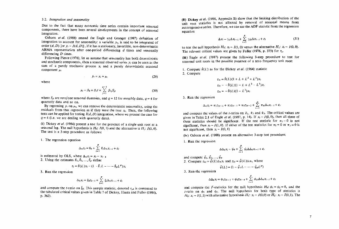
3.2. Integralion and seasonalily

Due to the fact that many economic time series contain important seasonal components, there have been several developments in the concept of seasonal integration.

Osborn el al. (1988) amend the Engle and Granger (1987) definition of integration to account for seasonality: a variable Yt, is said to be integrated of order (d, D) [or Yt - I(d, D)], if it has a stationary, invertible, non-deterministic ARMA representation after one-period differencing d times and seasonaIly differencing D times.

FolIowing Pierce (1976), let us assume that seasonality has both deterministic and stochastic components, then a seasonal observed series Yt can be seen as the sum of a purely stochastic process Xt and a purely deterministic seasonal component /lt

where

Yt= Xt + /lt

q-I

/lt = t30 + t3 ¡/ + ¿:; t3 2}S}t }=I

(29)

(30)

where S}t are zer%ne seasonal dummies, and q = 12 for monthly data, q = 4 for quarterIy data and so on. ~y regressing Yt on /lt, we can remove the deterministic seasonality, using the

reslduals from that regression as if they were the true Xt. Then, the foIlowing tests can be applied for testing I(d, D) integration, where we present the case for q = 4 (i.e. we are dealing with quarterIy data).

(i) Dickey el al. (1984) present a test for the presence of a single unit root at a seasonal lag. The nuIl hypothesis is Ho: 1(0,1) and the aIternative is HI: 1(0, O). The test is a 3-step procedure as foIlows:

1. The regression equation p

D.4Xt = 80 + ¿:; 8iD.4Xt-i + et i=1

is estimated by OLS, where ~4Xt = Xt - Xt-4 2. Using the estimates 81,82 , •.• , 8p define

Zt = 8(L )Xt = (1 - 81L - ... - 8pLP)xt

3. Run the regression p

D.4Xt = ~OZt-l + ¿:; ~iD.4Xt-i + et i=1

and compute the l-ratio on ~o. This sample statistic, denoted 7 1<4 is compared to the tabulated critical values given in Table 7 of Dickey, Hasza and FulIer (1984), p. 362).

COINTEORATIUN ANL1 UNll IU.lUIi:) ""VI

(li) Dickey el al. (1986, Appendix B) show that the limiting distribution of the unit root statistics is not affected by removal of seasonal means from autoregressive series. Therefore, we can use the ADF statistic from the regression equation

P

~Xt = 'YI~Xt-1 + ¿:; 'Y2i~Xt-; + et ;=1

(31)

to test the nulI hypothesis Ho: Xt - 1(1, O) versus the aIternative HI: Xt - 1(0, O). The relevant critical values are given by FuIler (1976, p. 373) for TI'-.

(iii) Engle et al. (1987) present the folIowing 3-step procedure to test for seasonal unit roots in the possible presence of a zero frequency unit root:

1. Compute 8(L) as for the Dickey et al. (1984) statistic 2. Compute

Zlt = 8(L)(1 + L + L 2 + L 3)xt

Z2t= -8(L)(1- L+ L2_ L 3)xt

Z3t= -8(L)(1- L 2 )xt

3. Run the regression p

D.4 Xt = 1I"1Zlt-1 + 1I"2Z2t-1 + 1I"3Z3t-2 + ¿:; 1I"4i~4Xt-i + et i=1

and compute the values of the t-ratios on 1ft, 11-2 and 1r3. The critical values are given in Table 2.1 of Engle el al. (1987, p. 14). If Xt - 1(0, O), then alI three of these statistics should be significant. If the test statistic for 11"1 = ° is not significant, then Xt - 1(1, O). If either of the test statistics for 11"2 = ° or 11"3 = ° is not significant, then Xt - 1(0, 1)

(iv) Osborn et al. (1988) present an alternative 3-step test procedure:

1. Run the regression p

D.D.4Xt = 1/10 + ¿:; 1/IiD.D.4 Xt- i + et ;=1

and compute 'f;1, 'f;2, ... , 'f;p 2. Compute Z4t = 'f;(L)D.4Xt and Z5t = 'f;(L)D.xto where

'f;(L) = (1 - 'f;IL - ... - 'f;pLP)

3. Run the regression P

D.~Xt = ePIZ4t-1 + eP2Z5t-4 + ¿:; eP3i~~Xt-i + et i=1

and compute the F-statistics for the nuIl hypothesis Ho: ePI = eP2 = 0, and the t-ratio on ePI and eP2. The nuIl hypothesis for both type of statistics is Ho: Xt - 1(1,1) with alternative hypothesis HI: Xt - 1(0,0) or H 2: Xt - 1(0,1). The

7

262 DOLADO, JBNKtNSON'AND SOSVILLA-IUVERO

critical values of these statistics are given in Table A.l of Osborn el al. (1988, p. 376).

4. Other forms of integration In this section, we review alternative forms of integration based upon the possibility that the model parameters are allowed to vary (periodic integration) or the possibility of using non-integer differencing orders to achieve stationarity in the data (fractional integration). BotlÍ ideas have received recent attention in the literature.

4.1. Periodic Inlegralion

Osborn el al. (1988), building upon the framework developed by Tiao and Grupe (1980), investigate the use of a periodic model (whose parameters are allowed to vary according to the time at which observations are made) as an alternative to the conventional approaches to modelling for seasonal data.

The non-deterministic periodic AR(1) process is given by the following expression

or

q

Yt = b WjSjtYt-1 + et j=1

(32)

(33)

when I falls in season j. As in equation (30), Sjt are seasonal dummy variables corresponding to season jU= 1, ... ,q). Equation (33) states that Yt is seasonal, seasonality arising not from any direct dependence of Yt on Yt-q, but from the annual variation in the autoregressive coefficients Wj. This dependence can arise, for example, if the allocation of expenditure over the year reflects seasonal tastes and hence seasonality in the underlying utility function (see Osborn, 1988).

Osborn el al. (1988) define periodic integration as follows: A variable Yt is periodically integrated of order one [or Yt - PI(1)] if Yt is non-stationary and ÓjYt is stationary, where the generalised difference operator Ój is defined as

ÓjYt = Yt - WjYt-1 (34)

the product WI, W2, •.. , Wq being equal to one. Osborn el al. (1988) propose two ways of testing for periodic integration:

(i) After regressing Yt on JLt (as defined in (30» to remove conventional deterministic seasonality, a non-deterministic periodic AR(1) pro ces s (as defined in (33» is fitted to the residuals Xt. This case is referred to as the removed deterministic seasonality case.

(ii) The case of inc1uded deterministic seasonality is given by fitting the

COINTEOaATIUN ANO UNIT ROOTS

following periodic AR(I) process to the original observations Yt

Yt = Oj + WjYt-i + et U = 1, ... , q)

To allow for the possibility of a periodic disturbance variance, they suggest a 2-step estimation procedure for both cases. In the first step, the appropriate eqUéition is estimated by OLS applied to observations on each of the q seasonal realisations, (i.e. four for quarterly data); then the equation is transformed by dividing each variable by the appropriate seasonal residual standard deviation estimated in this first stage regression. U sing the transformed data, in the second step the periodic AR(1) model is estimated in its two versions (i.e. removed and included deterministic seasonality), with imposition of the restriction W¡,W2, ... ,wq=l.

Finally, the tests (i) to (iii) in Section 3.2 are applied to the residuals of the periodic AR( 1) mode!.

4.2. Fractional inlegralion

As was seen in Section 2, one of the main characteristics of the existence of unit roots in the Wold representation of a time series is that they have 'long memory' (i.e. shocks have a permanent effect on the level of the series). In general it is known that the coefficient on et-j in the MA representation of any I(d) process has a leading term jd-I (for example, the coefficient in a random walk is unity, since d = 1). This implies that the variance of the original series is O(t2d-I). So, all that is needed to have 'long-memory', in the sense that the variance explodes as It 00, is a degree of differencing I di> 0.5. Thus, it is clear that a wide range of dynamic behaviour is ruled out a priori if d is restricted to integer values.

Granger and Joyeux (1980) and mOre recently Diebold and Rudebusch (1989) have proposed a new family of "long-memory" processes, denoted by ARFIMA (autoregressive fractionally integrated moving-average processes), of which the ARIMA processes are particular cases: A variable Yt is fractionally integrated of order d[or Yt - FI(d)] if Yt is non-stationary and Il d is stationary, where the operation Il d, using a binomial expansion, is as follows

(1- L)d= 1- dL + d(d-l) L2_ d(d-l)(d-2) L 3 + ... (35) 2! 3!

where d belongs to the rational set of numbers and d> 0.5. Note that these processes can always be constrained to belong to the open

interval (0.5,1.0) by subtracting the integer part of the differencing order. So if the degree of differencing is, for example, 1.7, we can always redefine the degree of differencing as d - 1 (0.7 in this case).

Diebold and Rudebusch (1989) propose the following method of testing and estimation for fractional integration:

(i) First difference the relevant series denoted Yt = (1 - L )Yt. As d of the level series equals 1 + d, a value of d equal to zero corresponds to a unit root in Yt.

8

Thus. we wish to estimate d in the model

(1- L)dYt = O(L)et

(ii) Estimate by OLS the following regression

In[I(Aj)] =(3o-{31In(4 sin 2 (Aj/2)J +f/j, j= 1, ... ,Tl/2

(36)

(37)

where Aj = 27rj/ TU = O, ... , T - 1) denote the harmonic ordinates of the sample and I(Aj) denote the periodogram at ordinate j (see Harvey, 1981, p.66). Geweke and Porter-Hudak (1983) prove that {JI is a consistent and asymptotically normal estimate of d. Furthermore, the variance of the estimate of (31 is given by the usual OLS estimator, which can be used to test the null hypothesis Ho: d = O [i.e. Yt - 1(1)] . Moreover they show that the variance of the disturbance f/j is known to be equal to 7r 2/6, which can be imposed to increase efficiency.

(iii) Given an estimate of d we transform the series Yt by the 'long-memory' filter (35), truncated at each point to the available sample. The transformed series is then modelled as in (36) (or in the ARMA representation) following the traditional Box and Jenkins (1970) procedure.

5. Testing for stationarity in the cointegrating residuals In the two previous sections we have discussed procedures to test for the order of integration of individual time series. This is, as we mentioned in Section 2, a first stage in the estimation and testing of cointegrating relationships. The reason is a matter of 'integration or growth accounting' in the words of Pagan and Wickens (1989) (i.e. the left and right hand sides of an equation, such as (4) must be of the same order of integration, otherwise, the residual will not be stationary). If for example, the dependent variable is 1(1), the independent variables need to be 1(1) and not cointegrate among themselves to an 1(0) variable or, perhaps, be 1(2) and cointegrate among themselves to an 1(1) variable.

In order to illustrate testing for cointegration, we will consider a bivariate case where say, Yt and Xt have been found to contain a single unit root at the regular frequency (i.e. both are 1(1». Then, the following part of the cointegration test is to estimate the cointegrating regression (4) and test whether the 'cointegrating residuals' (Zt = Yt - & - (JXt) are 1(0).

Engle and Granger (1987) suggest seven alternative tests for determining if Zt

is sta~ionary. Here we will consider only two of their suggested tests, namely the Durbm-Watson statistic for the cointegration equation (CRDW) and the ADF statistic for the cointegrating residual s (CRADF).

The DW statistic for equation (4) will approach zero if the cointegrating residuals contain an autoregressive unit root, and thus the test rejects the null hypothesis of non-cointegration if the CRDW is significantly greater than zero. The intuition underlying this test can be understood by means of a simple example. Suppose that Zt is assumed to follow an AR(1) process witn coefficient

:::OIN't1m~TtoN AND UNIT R.O~ 265

p. Then the null hypothesis of non-cointegration is Ho: p = l. Since it can be shown that the DW statistic is such that DW:::: 2(1 - p) (see, e.g. Harvey, 1981, p. 20), the previous null hypothesis can be translated into Ho: DW = O versus the alternative Hl: DW > O. Engle and Granger (1987, p. 269) present the critical values of this test for 100 observations.

The CRADF statistic is based upon the OLS estimation of p

~Zt = 'YtZt-l + ~ 'Y2i~Zt-i + et (38) ;=1

where again p is selected on the basis of being sufficiently large to ensure that et is a close approximation to white noise. The (-ratio statistic on 1'1 is the CRADF statistic. We cannot use the critical values tabulated by Fuller (1976) to test for a unit root in the cointegrating residuals. Intuitively, since OLS estimation of the cointegrating regression equation chooses a and (3 to mini mise the residual variance, we might expect to reject the null hypothesis Ho: Zt - 1(1) rather .more often than suggested by the nominal test size, so that the critical values have to be raised in order to correct the test bias. Engle and Granger (1987, p. 269) present the critical values for the CRADF statistic generated from Monte Carlo simulations of 100 observations.

Note that the critical values for both CRDW and CRADF statistics are for the bivariate case (i.e., for one dependent and one independent variable in the cointegrating regression), and for 100 observations. Engle and Yoo (1987) produce expanded critical values for CRDW and CRADF statistics for 50, 100 and 200 observations, and for systems of up to five variables.

6. Sorne new developrnents in cointegration In this section we survey sorne new test procedures for cointegration that have recently been proposed in the literature. Most of these procedures extend the testing and estimation approach introduced in Section 2 to a multivariate context where there may exist more than a single cointegrating relationship among a set of n variables. For example, among nominal wages, prices employment and productivity, there may exist two relationships, one determining employment and another determining wages (see, inter alia, Hall, 1986, and Jenkinson, 1986).

In general, if X t represents a vector of n 1(1) variables whose Wold representation is

~Xt= C(L)et (39)

where now et - nid(O, E), E being the covariance matrix of et and C(L) an invertible matrix of polynomial lags. If there exists a cointegrating vector a, then, premultiplying (39) by a' , we obtain

a' é1Xt = a' [C(1) + C*(L)(1- L)]et (40)

where C(L) has been expanded around L = 1 and C*(L) can be shown to be invertible (see Engle and Granger, 1987). If the linear combination a' X t is

9

266 DOLADO. lENKINSON ANO ~~VILLA-lt..VERO

stationary, then O!'C(1)=O and then (1- L) would cancel out on both sides of (40). If (39) is represented in AR form, we have that

A(L)C(L) = (1 - L)I (41)

where I is an identity matrix, and hence

A(1)C(1) = O (42)

This implies that A (1) can be written as A (1) = 'YO!' . If there were r cointegrating vectors (r ~ n - 1), then A (1) = Br' , where B and r are (n x r) matrices which collect the r different 'Y and O! vectors. Testing the rank of A(1) or C(1) constitutes the basis of the following procedures:

(i) Johansen (1988) and Johansen and Juselius (1988) develop a maximum likelihood estimation procedure that has several advantages on the 2-step regression procedure suggested by Engle and Granger. It relaxes the assumption that the cointegrating vector is unique and it takes into account the error structure of the underlying process.

Johansen considers the p-th order autoregressive representation of X t

(43)

which, following a similar procedure to the ADF test, can be reparameterised as

.::lXt = ñí.::lXt-, + ... + ñp-,.::lXt-p+, + ñpxt- p + et (44)

where ñp = -TI(1) (= - (TII + ... + TIp ». To estimate ñp by maximum-likelihood, we estimate by OLS the following regressions

.::lXt = rOI.::lXt-1 + ... + rOk-I.::lXt- k+1 + eOt

and

X t- p = rll.::lXt-1 + ... + rlk-I.::lXt-k+1 + elt

and compute the product moment matrices of the residual s T

Sij = T- ' ~ ei~Jt; i,} = 0,1 t=1

The likelihood ratio test statistic of the null hypothesis Ho: TIp = Br " i.e. there are at most r cointegrating vectors, is

p

-2In(Q)=-T ~ (1-).¡) (45)

where ).r+l, ... ,).p are the p - r smallest eigenvalues of SIOSOOSOI with respect to 8", obtained from the determinant

I ).SII - SIOSOOSOI I = O

Under the hypothesis that there are at most r cointegrating vectors, Johansen (1988) shows that the likelihood ratio test (45) is asymptotically distributed as a

COINTEGRATION AND UNIT ROOTS 267

functional f(W). Johansen (1988, p. 239) provides atable with various quantiles of the distribution of the likelihood ratio test for r = 1,2, ... , 5. He also shows that these quantiles can be obtained by approximating the distribution by cx2(f) where e = 0.85-0.85/f, and x2(f) is a central chi-square distribution with f= 2(p - r)2 degrees of freedom.

(ü) Stock and Watson (1988) focus on testing for the rank of C(1) in (40) and denote their approach as a 'common trends' approach, by noticing that if there exist r cointegrating vectors in (40), then there exists a representation such that"

where 4> is an nx(n - r) matrix and Tt is an n - r vector random walk. In other words, Xt can be written as the sum of n - r common trends and an 1(0) component. Estimating (39) as a multivariate ARMA (1, q) model, the null hypothesis that there are r cointegrating vectors is equivalent to the null hypothesis that there are n-r 'common trends'. This implies that, under the null hypothesis, the first (n - r) eigenvalues of the autoregressive matrix should be unity and the remaining eigenvalues should be smaller than one. The test is based on T()'n-r+1 - 1) and the critical values can be found in Stock and Watson (1988, p. 1104) .

Phillips and Ouliaris (1988) have also proposed a multivariate extension of their unit root test, as discussed in Section 3, based upon the eigenvalues of the long-run variance of the differenced multivariate series.

(üi) As discussed in Section 2, when concentrating on a single equation estimator in the case of a single cointegrating C(1,1) relationship, the OLS estimator of the slope in the static regression (4) is 'super-consistent' but its distribution is, in general, non-normal and in finite samples is biased (see Banerjee el al., 1986 and Gonzalo, 1989).

This bias and non-normality stem from the 1(1) character of the regressor and its possible correlation with the 1(0) disturbance Zt. Phillips (1988) has shown that in the case where Xt and Zt are independent at all leads and lags, the distribution is a 'mixture of normals' and, hence, the distribution of the l-statistic on {3 is asymptotically normal. Phillips and Hansen (1988) have developed an estimation procedure, equivalent to FIML, which corrects for the bias and yields asymptotic normality in the case where such correlation exists. The procedure, denoted as a 'fully modified estimator' (FME), is based upon a 'non-parametric' correction by which the error term Zt is conditioned on the process followed by .::lXt and, hence, orthogonality between regressors and disturbance is achieved by construction. The FME estimators of O! and (3 in (4) are given by

10

DOLADO, JENKINSON AND SOSVILLA-RIVERO

where X t = (1, Xt), e2 = (0,1)' and I T

~21 = T- 1 L; L; DoXt-d.t k=O t=k+l

the long-run variances obtained from the first-stage residuals Ze. as in Engle and Granger (1987). Notice that when O'J= Do21 = O the FME estimators coincide with OLS for the static regression (4).

It is interesting to notice that the FME procedure coincides with the Hendry-Sargan approach, as summarised in (3), through the ECM representation of dynamic single equation models, except when Zt or DoXt contain a moving-average disturbance in their respective representations. Even in that case it is possible to modify slightly equations like (3) by including leads of DoXt

in the regression model (see Saikkonen, 1989).

7. Brief conclusion The considerable gap between the economic theorist, who has much to say about equilibrium but relatively little to say about dynamics, and the econometrician, whose models concentrate on dynamic adjustment process, has, to some extent, been bridged by the concept of cointegration. In addition to allowing the data to determine the dynamics of the model, cointegration suggests that models can be significantly improved by introducing, and allowing the data to parameterise, equilibrium conditions suggested by economic theory. Furthermore, the generic existence of such long-run relationship can, and should, be tested, using the battery of tests for unit roots discussed in this paper.

Acknowledgements We are grateful to A. Banerjee, P. Burridge, A. Escribano, A. Espasa, J. Galbraith, D. Hendry and A. Maravall and an anonymous referee for their comments on previous versions of this paper. The usual caveat applies.

Notes 1. There is an early survey by two of us (see Dolado and Jenkinson, 1987) and a more

recent one by one of us (see Sosvilla-Rivero, 1989), and sorne excellent overviews by Granger (1986), Hendry (1986), Gilbert (1986), Stock and Watson (1987), Diebold and Nerlove (1988), Pagan and Wickens (1989) and Haldrup and Hylleberg (1989).

2. Even though cointegration implies at least one causal direction, it does not imply any explicit causal relationship. Here we have assumed that the causal relation suggested by the theory (i.e. XI causes YI) is the correct one. See Granger (1988) for a study of cointegration and causality.

3. Nickell (1985) shows that the ECM is also consistent with optimising behaviour on the part of economic agents.

COINTEGRA TION AND UNIT ROOTS

4. Alternatively we would say that a 'sup~r-consistent' estimator is such that i3 - {3 has probabilistic order of magnitude O(T- ~. ,. ., ., .

5. The explosivity of the variance charactenses the lOtegratlOn lO vanance . IntegratlOn can also be applied to other higher moments (see Escribano (1987) and Hansen (1988». . .

6. See the Appendix for a description for the sequentlal test procedure k(k ~ 2) umt roots. Note that the alternative sequence of testing for the presence of a unit root in the series levels and if it is not rejected, then test for a second unit root, Le. a unit root in the differences, and so on is not well founded on statistical grounds since the unit root tests described in Section 3 are based on the assumption of stationarity under the alternative hypothesis.

7. This result has been noticed by West (1988) and it is applicable al so to regression models like (2) where Xt has a unit root with drift. However, Hylleberg and Mizon (1989) have noted in simulation studies that the drift has to be quite large for the deterministic trend to dominate the integrated component. If there are two 1(1) regressors with drift in the model, a trend should also be included to avoid asymptotic perfect collinearity.

8. Ouliaris el al. (1988) compute critical values when in the maintained hypothesis there is up to a quintic trend. Similarly, Perron (1987) computes critical values when there is a piecewise linear trend under the maintained hypothesis. .

9. Sims el al. (1986) and Banerjee and Dolado (1988), have shown that the estImates of coefficients on 1(0) variables in regression mode1s with 1(1) variables are 0(T

1I2) and

asymptotically normally distributed. 10. In the frequency domain notation, the long-run variance is equal to 27r!e(0), where

!e(O) in the spectrum of el evaluated at frequency zero. 11. The size of C(I) in a univariate context, has been called the 'size the unit root', giving

rise to a literature (see Cochrane (1988) and references therein) which deals with the relative importan ce of the trend and cyclical components in the decomposition of a time-series.

Appendix: testing for k unit roots Dickey and Pantula (1987) suggest a sequence of tests for unit roots, starting with the largest number of roots under consideration (k) and decreasing by one each time the null hypothesis is rejected, stopping the procedure when the null hypothesis is accepted.

They illustrate their sequential procedure for the case k = 3. It is as follows:

1. Run the regression

Do 3Yt = ~O + ~lDo2Yt-l + Ct

(where Do 3 denotes third difference), and compute the 'pseudo t-statistic' ti,n (3) (i.e. the t-statistic on ~¡). Reject the null hypothesis H3 of three unit roots and go to step 2 if ti,n(3) < T/L (or ti,n(3) > T/L if absolute values are considered) where T/L is given by Fuller «1976), p. 373).

2. Run the regression

Do 3Yt = ~6 + ~íDo2Yt_l + ~2DoYt-l + Ct

and compute ti,n(3) and ti,n(3). Reject the null hypothesis H 2 of exactly two unit

11

270 DOLADO, JENKINSON AND SOSVlLLA-RIVERO

roots and go to step 3 if in addition to t:.n(3) < TI' it is also found that t:'n(3) < TI'

3. Run the regression

~ 3 Yt = ~ó + ~r~ 2 yt-I + ~!~Yt-I + ~jYt-1 + et

and compute t~n(3), ti:n(3) and t~n(3). Reject the null hypothesis HI of exactly one unit root in favour of the hypothesis Ho if ttn (3) < TI' (i = 1,2, 3).

References Banerjee, A. and Dolado, J. (1988) Tests of the life cycle permanent income hypothesis

in the presence of random walks: Asymptotic theory and small-sample interpretations. Oxford Economic Papers 40, 610-633.

Banerjee, A., Dolado, J., Hendry, D. and Smith G. (1986) Exploring equilibrium re1ationships in econometrics through static models: Sorne Monte-Cario evidence. Oxford Bulletin of Economics and Statistics 48, 253-277.

Bhargava, A. (1986) On the theory of testing for unit roots in observed time series. Review of Economic Studies 53, 369-384.

Box, G. and Jenkins, G. (1970) Time Series Analysis, Forecasting and Control. San Francisco: Holden-Day.

Cochrane, J. (1988) How big is the random walk in GNP? Journal of Political Economy 96, 893-920.

Davidson, J., Hendry, D., Srba, F. and Yeo, S. (1978) Econometric modeUing of the aggregate time-series relationship between consumers' expenditure and income in the United Kingdom. Economic Journal 88, 349-363.

Dickey, D. and Fuller, W. (1979) Distribution of the estimators for autoregressive time-series with a unit root. Journal of the American Statistical Association 74, 427-431.

-- (1981) Likelihood ratio statistics for autoregressive time series with a unit root. Econometrica 49, 1057-1072.

Dickey, D. and Pantula, S. (1987) Determining the order of differencing in autoregressive processes. Journal of Business and Economic Statistics 15, 455-461.

Dickey, D., Bell, W. and Miller, R. (1986) Unit roots in time series models: Tests and implications. The American Statistician 40, 12-26.

Dickey, D., Hasza. D. and Fuller, W. (1984) Testing for unit roots in seasonal time series. Journal of the American Statistical Association 79, 355-367.

Diebold, F. and Nerlove, M. (1988) Unit roots in economic time series: A selective survey. Discussion Paper No. 49. Federal Reserve Board. Washington D.C.

Diebold, F. and Rudebusch, G. (1989) Long memory and persistence in aggregate output. Journal of Monetary Economics 24, 189-209.

Dolado, J. (1989) Optimal instrumental variable estimator of the AR parameter of an ARMA (1,1), mimeo, (forthcoming in Economic Theory).

Dolado, J. and Jenkinson, T. (1987) Cointegration: A survey of recent developments. Applied Economics Discussion Paper No. 39. University of Oxford.

Engle, R. and Granger, G. (1987) Cointegration and error correction: Representation, estimation and testing. Econometrica 55, 251-276.

Engle, R., Granger, C., Hylleberg, S. and Yoo, S. (1987) Seasonal integration and cointegration. Discussion Paper No. 88-32. University of S. Diego.

Engle, R. and Yoo, S. (1987) Forecasting and testing in cointegrated systems. Journalof Econometrics 35, 143-159.

Escribano, A. (1987) Cointegration, time co-trends and error correction systems: An alternative approach. CORE Discussion Paper No. 8715. University of Louvain.

-

COINTEGRA TION AND UNIT ROOTS

Fuller, W. (1976) Introduction to Statistical Time Series. New York: John Wiley and Sonso

Geweke, J. and Porter-Hudak, S. (1983) The estimation and application of long memory time series models. Journal of Time Series Analysis 4, 221-238.

Gilbert, C. (1986) Professor Hendry's econometric methodology. Oxford Bulletin of Economics and Statistics 48, 283-307.

Gonzalo, J. (1989) Comparison of five alternative methods ~f estimati~g l<?ng-run equilibrium relationships. Discussion Paper 89-55. Universlty of Cahforma, San Diego.

Granger, C. (1981) Sorne properties oftime series data and their use in econometric model specification. Journal of Econometrics 28, 121-130.

__ (1986) Developments in the study of cointegrated economic variables. Oxford Bulletin of Economics and Statistics 48, 213-228.

__ (1988) Sorne recent developments in a concept of causality. Journal of Econometrics 39, 199-211.

Granger, C. and Newbold, P. (1974) Spurious regressions in econometrics. Journalof Econometrics 26, 1045-1066.

Granger, C. and Joyeux, R. (1980) An introduction to long memory time series models and fractional integration. Journal of Time Series Analysis, 1, 15-39.

Granger, C. and Weiss, A. (1983) Time series analysis of error correction models, in Karlin, S., Amemiya, T. and Goodman, L. (eds) , Studies in Economic Time Series and Multivariate Statistics, New York: Academic Press.

Haldrup, N. and Hylleberg, S. (1989) Unit roots and deterministic trends, with yet another comment on the existence and interpretation of a unit root in U.S. GNP, mimeo. University of Aarhus.

Hall, A. (1989). Testing for a unit root in the presence of moving average errors. Biometrika 76, 49-56.

Hall, S. (1986) An application of the Engle and Granger two-step estimation procedure to U.K. aggregate wage data. Oxford Bulletin of Economics and Statistics 48, 229-240.

Hannan, E. (1970) Multiple Time Series. New York: Wiley. . . Hansen, B. (1988) A model of heteroskedastic cointegration, mimeo. Yale Umverslty. Hansen, B. and Phillips, P. (1988) Estimation and inference in models of cointegration:

A simulation study. Cowles Foundation Discussion Paper No. 881. Yale University. Harvey, A. (1981) Time Series Models. Oxford: Phillip Allan. Hendry, D. (1986) Econometric modelling with cointegrated variables: An overview.

Oxford Bulletin of Economics and Statistics 48, 201-212. Hendry, D. and Mizon, G. (1978) Serial correlation as a convenient simplification not a

nuisance: A cornrnent on a study of the demand for money by the Bank of England. Economic Journal 88, 349-363.

Hendry, D. and Richard, J. F. (1983) The econometric analysis of economic time series. International Statistical Review 51, 111-163.

Hylleberg, S. and Mizon, G. (1989) A note on the distribution of the least squares estimation of a random walk with drift. Economics Letters 29, 225-230.

Jenkinson, T. (1986) Testing neo-classical theories of labour demand: An application of cointegration techniques. Oxford Bulletin of Economics Statistics 48, 241-251.

Johansen, S. (1988) Statistical analysis of cointegration vectors. Journal of Economic Dynamics and Control 12, 231-254.

Johansen, S. and Juselius, K. (1988) Hypothesis testing for cointegration vector s with an application to the demand for money in Denmark and Finland. Working Paper No. 88-05. University of Copenhagen. .

Molinas, C. (1986) A note on spurious regressions with integrated moving average errors. Oxford Bulletin of Economics and Statistics 48, 279-282.

12

272 DOLADO, JENKINSON ANO SOSVILLA-RIVERO

Nelson, C. and Kang, H. (1981) Spurious periodicity in inappropriately detrended time series. Econometrica 49,741-751.

Nelson, C. and Plosser, C. (1982) Trends and random walks in macroeconomic time series. Journa! 01 Monetary Economics 10, 139-162.

Newey, W. and West, K. (1987) A simple, positive semi-definite heteroskedasticity and autocorrelation consistent covariance matrix. Econometrica 55, 703-708.

Nickell, S. (1985) Error correction, partial adjustment and aH that: An expository note. Oxlord Bulletin 01 Economics and Statistics 47, 119-129.

Osborn, D. (1988) Seasonality and habit persistence in alife cycle model of consumption. Journa! 01 Applied Econometrics 3, 255-266.

Osborn, D., Chui, A., Smith, J. and BirchenhaH, C. (1988) Seasonality and the order of integration for consumption. Oxlord Bulletin 01 Economics and Statistics 50, 361-377.

Ouliaris, S., Park, J. and Phillips, P. (1988) Testing for a unit root in the presence of a maintained trend (forthcoming in B. Raj (ed) Advances in Econometrics and Modelling. Needham: Kluwer Academic Press).

Pagan, A. and Wickens, M. (1989) A survey of sorne recent econometric methods. Economic Journal, 99, 962-1025.

Park, J. and Phillips, P. (1988) Statistical inference in regression with integrated processes: Part l. Econometric Theory 4, 468-497.

Perron, P. (1987) The great crash, the oil price shock and the unit root hypothesis. Cahier 8749. University of Montreal (forthcoming in Econometrica).

Phillips, P. (1986) Understanding spurious regression in econometrics. Journa! 01 Econometrics 33, 311-340.

-- (1987) Time series regression with a unit root. Econometrica 55, 277-301. -- (1988) Optimal inference in cointegrated systems. Cowles Foundation Discussion

Paper No. 866. Yale University. Phillips, P. and Ouliaris, S. (1988) Testing for cointegration using principal components

methods. Journa! 01 Economic Dynamics and Control 12, 205-230. Phillips, P. and Perron, P. (1988) Testing for a unit root in time series. Biometrika 75,

335-346. Pierce, D. (1976) Seasonality adjustment when both deterministic and stochastic

seasonality are present, in A. Zellner (ed) Seasona! Ana!ysis 01 Economic Time Series. Washington: Bureau of the Census.

Said, S. and Dickey, D. (1984) Testing for unit roots in autoregressive-moving average models of unknown order. Biometrika 71, 599-607.

-- (1985) Hypothesis testing in ARIMA (p, q, q) models. Journa! 01 the American Statistica! Association 80, 369-374.

Saikkonen, P. (1989) Asymptotically efficient estimation of cointegration regressions. Research Report No. 72, University of Helsinki.

Sargan, J. (1964) Wages and prices in the UK: A study in econometric methodology, in Hart, P., Milis, G. and Whittaker, J. (eds.) Econometric Ana!ysis lor Nationa! P!anning, London: Butterworths.

Schwert, G. (1987) Effects of model specification on tests for unit roots in macroeconomic data. Jouma! 01 Monetary Economics 20, 73-103.

-- (1989) Tests for unit roots. A Montecarlo investigation. Journa! 01 Business and Economic Statistics 7, 147-159.

Sims, C., Stock, J. and Watson, M. (1986) Inference in linear time-series models with sorne unit roots, mimeo (forthcoming in Econometrica).

Sosvilla-Rivero, S. (1989) Cointegration and unit roots: A survey. Discussion Paper 89-5, University of Birmingham.

Stock, J. (1987) Asymptotic properties of least squares estimators of cointegrating vectors. Econometrica 55, 381-386.

COINTEGRA TION ANO UNIT ROOTS 273

Stock, J. and Watson, M. (1987) Variable trends in economic time series. Journalol Economic Perspectives 2, 147-174.

__ (1988) Testing for common trends. Journa! 01 the American Statistica! Association. 83, 1094-1107.

Tiao, G. and Grupe, M. (1980) Hidden periodic autoregressive-moving average models in time-series data. Biometrika 67, 365-373.

West, K. (1988) Asymptotic normality when regressors have a unit root. Econometrica 56, 1397-1417.

Wold, H. (1938) A study in the Ana!ysis 01 Stationary Time-Series. Stockholm: Almguist and WikneH.

13