coincidence of storm surges and river discharges due to ... · 3 coincidence of storm surges and...
TRANSCRIPT

Coincidence of storm surges and river discharges
due to typhoons in the Pampanga delta
Master Thesis
H.J. aan het Rot

2
Cover image: Satellite image of Typhoon Nesat in 2011 above the Pampanga delta (NASA, 2011).

3
Coincidence of storm surges and river discharges
due to typhoons in the Pampanga delta
Master Thesis
Herm Jan aan het Rot
University of Twente
Faculty of Engineering Technology
Department of Water Engineering and Management
P.O. Box 217
7500 AE Enschede
The Netherlands
Author:
Herm Jan aan het Rot
Supervisors:
Prof. dr. J.C.J. Kwadijk University of Twente
Dr. ir. M.J. Booij University of Twente
Dr. ir. J.V.L. Beckers Deltares
Delft, Oktober 2018

4
SUMMARY
The Pampanga delta (Philippines) is due to its geographical location prone to typhoons which can
result in extreme discharges and storm surges in Manila Bay. In most flood risk studies, river discharges
and storm surges are considered independent, but if there exists dependence between storm surges
and river discharges, this might have a significant influence on design levels and expected inundations.
Previous studies showed the importance of taking into account the joint occurrence of storm surges
and high discharges for different regions in the world, but the importance differs per catchment.
In this study, the importance of taking into account the coincidence of storm surges and discharges in
exposure and risk studies in the Pampanga delta has been explored. This study shows that there is an
average time lag of 36 hours between the occurrence of storm surge and discharge peaks in the
Pampanga delta, which seems to decrease when both peaks are more extreme. There is also a clear
shift in the probability distribution of the storm surges during extreme discharge events in comparison
with independent events, resulting in significantly higher storm surges during extreme discharge
events. It was also shown that there is an increased probability of joint occurrence of extreme
discharges and extreme storm surges in comparison with the independent probability.
The effect of the joint occurrence of extreme storm surges and extreme discharges on inundations is
investigated based on inundation maps of hypothetical scenarios with different combinations of storm
surge, tide and discharge. With these scenarios, the importance of storm surge, river discharge, tide
and the timing of those components relative to each other were investigated. The inundation maps
are simulated by the hydrodynamic model Delft3D-FLOW. The forcing data that is used in Delft3D-
FLOW consists of river discharges and wind and pressure fields that are derived from historical
typhoon tracks from the Joint Typhoon Warning Centre (JTWC). The discharge input for the rivers is
determined by hydrological simulations in wflow, which is a hydrological model developed by Deltares
based on the PCRaster Python framework. The wflow model for the Pampanga has been calibrated
using water level measurements by the Pampanga River basin Flood Forecasting and Warning Centre
(PRFFWC) and a rating curve for the measurement station at Mount Arayat.
The results of the hydrodynamic simulations in Delft3D-FLOW show that the inundation extent and
depth are dominated by the discharge. But neglecting the joint occurrence of storm surges and high
discharges (with both an estimated return period of five years) results in an underestimation of the
inundations over a large area. The underestimation of the inundation depth reaches up to 30 cm in
Highlights
- Taking into account the joint occurrence of storm surges, discharge peaks and high tides
is of major importance in exposure and risk studies in the Pampanga delta;
- Simulated inundations in the largest part of the Pampanga delta are dominated by river
discharges but can be strengthened by storm surges;
- In some areas in the surroundings of Manila Bay and in north-western Manila the
simulated inundations are dominated by the combination of storm surges and tides;
- There is a significant increase of the joint probability of extreme storm surges and
extreme discharges in comparison with the independent probability.

5
the north-western part of the Pampanga delta and more than 50 cm on a local scale in the
surroundings of Manila Bay. Without the extreme river discharges, the simulated inundations are
restricted to some parts in the surroundings of Manila Bay and some parts in north-western Manila.
Furthermore, the results show that the timing of the tide with respect to the storm surge has a
significant influence on the inundation depth over a large area in the Pampanga delta.
Due to the uncertainties in the hydrological simulation, the Digital Elevation Model, and the wind and
pressure fields that are used to force Delft3D-FLOW, the conclusions about the exact inundation depth
and inundation extent are uncertain. Nevertheless, it can be concluded that the inundations are
dominated by the river discharges. Furthermore, based on the significant differences in the simulated
inundations with and without storm surge, it can be concluded that neglecting the joint occurrence of
storm surges, discharge peaks and high tides results in an underestimation of the inundation depth
over a large area and the inundation extent on a local scale.
Based on the conclusions of this research, it is recommended to take into account the joint occurrence
of storm surges, discharge peaks and high tides in exposure and risk studies in the Pampanga delta.
To mitigate flooding, it is recommended to explore the possibilities to increase the time lag between
the storm surge and discharge peaks and that cut-off the discharge peaks itself. It is also highly
recommended to take into account the extraordinary land subsidence and sea level rise in exposure
and risk studies in the surroundings of Manila Bay since it will probably result in more severe
inundations due to storm surges in the future.

6
PREFACE This thesis is the final part of my study Civil Engineering and Management at the University of Twente.
During this research, the joint occurrence of storm surges and high river discharges due to typhoons
was investigated. It was an exciting experience to work on such an interesting and relevant topic and
to deal with the limitations of doing research on extreme events. Especially dealing with the issues
regarding the data reliability and the available models was a huge challenge. Without the never-
ending support of my supervisors, finishing this research was not possible. Jaap Kwadijk, Martijn Booij
and Joost Beckers, I am very grateful for your pragmatic advice, support and for taking the time to
reflect on the process and the report.
Furthermore, I would like to thank my colleagues at Deltares for the pleasant time I had and their help
during this research. I have good memories of the lunches, the coffee talks, climbing the stairs up to
the 7th floor as fast as possible after lunch and especially the indoor soccer tournament of Deltares. In
particular, I would like to thank Deepak Vatvani and Roman Schotten for their support with Delft3D-
FLOW and FEWS, respectively.
In addition, special thanks to Joeri Massa for working together on almost all assignments we faced
during our study, I think we were a good team. Finally, I would like to thank my parents, family and
friends for their never ending support.
Herm Jan aan het Rot
Delft, Oktober 2018

7
CONTENTS Summary ................................................................................................................................................. 4
Preface .................................................................................................................................................... 6
List of abbreviations ................................................................................................................................ 9
1. Introduction .................................................................................................................................. 10
1.1. Background ........................................................................................................................... 10
1.2. State of the art ...................................................................................................................... 11
1.3. Research gap ......................................................................................................................... 12
1.4. Research objective and questions ........................................................................................ 13
1.5. Thesis outline ........................................................................................................................ 13
2. Case study ..................................................................................................................................... 14
2.1. Manila Bay ............................................................................................................................. 14
2.2. Pampanga River basin ........................................................................................................... 15
2.3. Typhoons affecting Manila Bay ............................................................................................. 17
2.4. Models .................................................................................................................................. 18
2.5. Used time series .................................................................................................................... 21
3. Method ......................................................................................................................................... 22
3.1. River discharge ...................................................................................................................... 22
3.2. Storm surge ........................................................................................................................... 26
3.3. Effects of joint occurrence .................................................................................................... 28
4. Results ........................................................................................................................................... 31
4.1. River discharge ...................................................................................................................... 31
4.2. Storm surge ........................................................................................................................... 37
4.3. Effects of joint occurrence .................................................................................................... 44
5. Discussion ...................................................................................................................................... 57
5.1. Potential of this research ...................................................................................................... 57
5.2. Limitations............................................................................................................................. 58
5.3. Challenges ............................................................................................................................. 61
6. Conclusions ................................................................................................................................... 62
6.1. Conclusions on the effect of typhoons on discharges and subsequent inundations in the
Pampanga delta ................................................................................................................................ 62
6.2. Conclusions on the effect of typhoons on storm surges in Manila Bay and subsequent
inundations in the Pampanga delta .................................................................................................. 62
6.3. Conclusions on the effect of joint occurrence of storm surges and discharge peaks on
inundations in the Pampanga delta .................................................................................................. 62

8
6.4. General conclusions .............................................................................................................. 63
7. Recommendations ........................................................................................................................ 64
7.1. Recommendations for further research ............................................................................... 64
7.2. Recommendations for policy makers and water managers ................................................. 65
8. Bibliography .................................................................................................................................. 66
A. Appendix ....................................................................................................................................... 71
A.I. Selecting input data for the wflow simulations .................................................................... 71
A.II. Calibration and validation of the wflow model .................................................................... 81
A.III. Inundation simulations with the lowest discharge boundary .............................................. 97

9
LIST OF ABBREVIATIONS AET Actual evapotranspiration AMC Antecedent Moisture Condition CDF Cumulative Distribution Function CN Curve Number DEM Digital Elevation Model E2O EartH2Observe Fr Froude number GPD Generalized Pareto Distribution JICA Japan International Cooperation Agency JTWC Joint Typhoon Warning Centre KS Kolmogorov-Smirnov (test) MSWEP Multi-source Weighted-Ensemble Precipitation NS Nash-Sutcliffe (coefficient) PDF Probability Density Function POT Peaks over Threshold PRFFWC Pampanga River basin Flood Forecasting and Warning Centre RVE Relative Volume Error SRTM Shuttle Radar Topography Mission TRMM Tropical Rainfall Measuring Mission UHSLC University of Hawaii Sea Level Centre WES Wind Enhance Scheme for cyclone modelling WFDEI WATCH-Forcing-Data-ERA-Interim

10
1. INTRODUCTION
1.1. Background In the coastal and inter-tidal zones, the joint occurrence of storm surges and high river discharges can
lead to increased flood severity, duration or frequency in comparison with the situation where storm
surges or high river discharges happen separately. The interaction between these events is generally
referred to as coincident or compound events (IPCC, 2012) or as joint dependence (Westra, 2018).
Compound events are a special category of climate extremes, which result from the combination of
events. According to the Intergovernmental Panel on Climate Change (IPCC, 2012), compound events
in climate science can be (1) two or more extreme events occurring simultaneously or successively, (2)
combinations of extreme events with underlying condition that amplify the impact of the events, or
(3) combinations of events that are not extreme by themselves but lead to an extreme event when
they are combined.
Understanding the risk posed by compound events is likely to become more important in the future
due to sea level rise and changing tidal regimes (Petroliagkis et al., 2016). Towns close to estuaries
and tidal rivers are at risk from the combination of tidal and fluvial flooding. The expected sea level
rise in combination with an increase in extreme precipitation events and the increasing urbanization
in low-lying areas is expected to create major flood risk problems for many estuarine and coastal
towns (Petroliagkis et al., 2016).
An important component in the assessment of compound events is to understand the historical
relationship between different physical factors like precipitation, river discharge, storm surge,
astronomical tide, wind and wave setup. Assumptions are often made about the coincidence of the
different factors, leading to an under or overestimation of the probability of flooding (Petroliagkis et
al., 2016). In reality, some events may have compounding consequences when they occur
simultaneously, while others may occur independently from others. Petroliagkis et al. (2016) state:
“source variables in most cases are not independent as they may be driven by the same weather event,
so their dependence, which is capable of modulating their joint return period, has to be estimated
before the calculation of their joint probability”. Taking into account these compounding
consequences is important in determining probabilities of the events and might have a significant
influence in determining design levels and expected inundations.
Deltares is conducting a study that focuses on inundations caused by extreme precipitation events on
land combined with storm surges due to tropical storms or tropical typhoons in South East Asia.
Comparison of the number of storm and typhoon occurrences in Myanmar (Yangon), Bangladesh and
the Philippines (Manila) shows that Manila is hit with the highest frequency (Vatvani, 2016). In the
region of Manila, floods that are caused by a combination of fluvial and tidal flood events happen
quite regularly. Furthermore, the floods result in severe damages to houses, roads, rice paddies and
fishponds resulting in major economic damage (Van ’t Veld, 2015). Therefore, Manila Bay was selected
as a case study to investigate the probability of joint occurrence of storm surges and river discharges
during typhoons.
The Philippines is on average affected by nine tropical cyclones every year. These cyclones result in
extreme precipitation events and extreme river discharges. In Figure 1, the water level at Manila Bay
(UHSLC, 2018) and (simulated) discharge of the Pampanga River during typhoon Nesat (2011) are

11
presented. From Figure 1 it becomes clear that there is a time lag between the storm surge and the
discharge peak. Internal research at Deltares (Vatvani, 2016) showed that during Typhoon Nesat the
combined effect of extreme river discharge and storm surge resulted in severe inundations in the
Pampanga delta. Taking into account the joint occurrence of storm surge and discharge peaks was
important in simulating the inundations due to Typhoon Nesat.
Figure 1 Discharge of the Pampanga River and water level in Manila Bay during Typhoon Nesat as used by Vatvani (2016).
1.2. State of the art Since the start of this millennium, quite some research has been conducted on the joint occurrence of
storm surges and river discharges or precipitation. Svensson and Jones (2004; 2002) conducted
multiple studies on the “dependence between extreme sea surge, river flow and precipitation” in
Great Britain. They showed that dependency between river discharges and storm surges occurred in
some areas in South and West Britain but not everywhere. They found higher dependencies in
catchments in hilly areas with a southerly to westerly aspect (Svennson & Jones, 2004). Quick
hydrological response to the abundant precipitation in these sloping catchments resulted in an arrival
of the flow peak in the estuary on the same day as the storm surge. Furthermore, Svennson & Jones
(2004) conclude that in some areas the higher soil moisture deficits in summer, inhibiting direct runoff,
may be the reason for higher dependencies in the winter than in the summer. Other areas may be less
affected by this soil moisture deficit and are more influenced by storm tracks in the summer, resulting
in higher dependencies in the summer than in the winter. Svennson & Jones (2004) also stated that
dependence between river flow and storm surge can vary over short distances. This has to do with the
fact that river response depends on catchment characteristics such as area and geology.
Zheng et al. (2014; 2013) also conducted research on the dependence between extreme precipitation
and storm surges in Australia. They showed that statistically significant dependence was observed for
the majority of the analysed locations. Furthermore, they stated that this dependency showed
regional and seasonal variation and that this dependence can remain significant at distances (between
the storm surge and precipitation measurement station) of several hundred kilometres. Based on that
observation they conclude that: “dependence arises largely due to synoptic scale meteorological
forcing” (Zheng et al., 2013). They also showed that the dependence strength varies with the time lag
between extreme precipitation and the storm surge events. They conclude that the two processes
must be considered jointly in flood risk assessment to be quantified correctly.
-1
-0.5
0
0.5
1
1.5
0
500
1000
1500
2000
2500
3000
25-09-11 26-09-11 27-09-11 28-09-11 29-09-11 30-09-11
Wat
er
leve
l (m
)
Dis
char
ge (
m^3
/s)
Discharge Water level

12
Klerk et al. (2015) conducted a study on the coincidence of storm surges and extreme discharges
within the Rhine-Meuse Delta. In their study, they found dependence between the discharges at
Lobith and storm surges at Hoek van Holland, with the highest dependence for a time lag of six days
between the two processes. For cases without a time lag, there was no significant dependence found,
so there is no need for considering dependence in flood protection and policy-making in their study
area.
Morin et al. (2016) showed that the storm surge level in Manila Bay is related to the minimum distance
between the typhoons eye and Manila Bay. Typhoons that crossed Manila Bay more than 50
kilometres to the south never resulted in moderate (0.41-0.6m) or severe (>0.6m) storm surges. In
contrast, typhoons crossing to the north of Manila Bay can result in moderate storm surges up to a
distance of 400 km. They also showed that the storm intensity can influence the storm surge.
The importance of taking into account storm surge and river discharge at the same time in inundation
modelling in the Tsengwen River basin in Taiwan was shown by Chen and Liu (2014). They studied the
impact of storm surge only, river discharge only and the effect of storm surge combined with
discharges for super typhoon Haiyan (with adapted pathway). They found a significant increase of the
inundated area for the compound flooding, which was 60 km2 for surge only, 30 km2 for discharge
(T=200 year) only and 96 km2 for the compound flooding. The maximum flooding depth for the surge
and compound flood were equal (+/- 1.98 m) while the flooding depth due to discharge only was 1.58
m.
Vatvani (2016) conducted research on the inundations in the Pampanga delta due to storm surge and
discharge during Typhoon Nesat (2011). The results show that excluding storm surge from the
simulations lead to an underestimation of the inundations. He also showed that the inundations are
concentrated in the Pampanga delta in the area between the Pampanga main river and the Angat
River.
The risk of compound flooding will increase in the future due to climate change. Fluvial floods will
increase in large parts of the world and more intense storm surges can be expected (Ikeuchi et al.,
2017). Also, the rising sea level and rising sea temperature can result in increased flood extent and
depth (Karim & Mimura, 2008).
1.3. Research gap Manila is located in South East Asia in a region that is prone to typhoons. These typhoons can induce
storm surges generated by wind set-up, wave set-up and pressure set-up. Furthermore, typhoons
induce extreme precipitation events, which lead to extreme discharges.
Since dependencies between storm surges and discharges vary between catchments (Svennson &
Jones, 2004; Svensson & Jones, 2002), it is not possible to draw conclusions on the importance of
taking into account the joint occurrence based on studies in other areas. Therefore, research with a
case study in the Pampanga delta is necessary to draw conclusions on the importance of taking into
account the joint occurrence in exposure and risk studies in the Pampanga delta.
Vatvani (2016) showed that taking into account storm surges and river discharges resulted in increased
inundations in the Pampanga delta during Typhoon Nesat in 2011, compared to a simulation with only
river discharge. But from this single event, it cannot be concluded whether it is always important to

13
take into account the discharges and storm surges in determining flood hazard and inundations. The
circumstances during Typhoon Nesat could have been very unusual.
To draw general conclusions, it has to be investigated whether there is a correlation between the
occurrence of storm surges and the occurrence of discharge peaks or that the storm surges and
discharges occur independently of each other. It also has to be investigated how large the time lag
between the storm surge and the discharge peaks is and if there is an increased probability of
simultaneous occurrence of discharge and storm surge peaks during extreme events in comparison
with the independent probability.
The extensive inundations that occurred during Typhoon Nesat do not necessarily mean that there is
a need to take into account coincidence and dependency between storm surges and discharges in
general. It is not known what the relative influence of the discharge and the storm surge is on the
inundation extent and inundation depth. It could be that the inundations are dominated by the
combination of storm surge and tide and that the discharge has only a minor influence or the other
way around. It also remains to be investigated what is the reason why some areas are influenced more
by the joint occurrence than other areas.
1.4. Research objective and questions The objective of this research is:
To determine the influence of coincidence of extreme storm surges and extreme discharge peaks due
to typhoons on inundations in the Pampanga delta.
To achieve this research objective, the following sub-questions will be answered:
1. What is the effect of typhoons on river discharges and subsequent inundations in the
Pampanga delta?
2. What is the effect of typhoons on storm surges in Manila Bay and subsequent inundations in
the Pampanga delta?
3. What is the effect of the joint occurrence of storm surge and discharge peaks on inundations
in the Pampanga delta?
1.5. Thesis outline In chapter 2, important information about the Pampanga delta and Manila Bay is provided together
with some background information about typhoons that affect the Pampanga delta and Manila Bay.
Further, a description of the hydrological wflow model and the hydrodynamic Delft3D-FLOW model
and the datasets that were used, are given in chapter 2. In chapter 3, the method is given that will be
applied to answer the research questions and in chapter 4 the results are presented. In chapter 5 the
results of this research are discussed, in chapter 6 the conclusions are drawn and in chapter 7 the
recommendations are given.

14
2. CASE STUDY Manila Bay and the Pampanga delta were chosen as case study to investigate the probability of joint
occurrence of storm surges and river discharges. Therefore, first, some background information about
Manila Bay and the Pampanga delta is given in section 2.1 and 2.2 respectively. Thereafter a
description about typhoons affecting Manila Bay and the Pampanga delta is given in section 2.3 and
the models that will be used in this research are shortly described in section 2.4. Finally, an overview
of the data that will be used in the analyses and as input for the models is given in section 2.5.
2.1. Manila Bay Manila Bay is situated in the Western Philippines, roughly between 120°30’E to 121°E and 14°15'N to
14°50'N (Figure 2). The semi-enclosed basin is bounded by the provinces Cavite, Bulacan, Pampanga
and Bataan and in the East by the cities of Metro Manila. It has an area of 1994 km3, a maximum length
of 19 km and a maximum width of 48
km. The average depth of the bay is 17
meters and the total length of the
coastline is 190 km (Perez et al., 1996).
The estimated total volume of Manila
Bay is 28.9 billion cubic meters. The
mouth of Manila Bay is divided by an
island into two parts, one of 3.2 km on
the North side and one of 10.5 km
wide on the Southside. The total area
that drains into Manila Bay is
approximately 17,000 km2, of which
10,540 km2 is contributed by the
Pampanga River basin which consists
of the Pampanga main river, the Pasac
River and the Angat River.
The Pasig River basin adds another 4678 km2 and is actually a tidal estuary which connects Manila Bay
with Laguna de Bay. Morin et al. (2016) stated that the Philippines experiences monsoon winds over
the entire year, with north-easterly winds during the winter and south-westerly winds during the
summer. During the summer period (June to September) the south-westerly monsoon resulted in
wind speeds up to 10 m/s and entered the Bay from a south-southwest direction. The bay experiences
a relatively dry season between December and May and a wet season between June and September.
Measurements show an overall relative sea level rise of approximately 0.8 m between 1960 and 2012
(Morin et al., 2016). Within this rise also land subsidence is considered, which is extremely relevant
since the land in Metro Manila is sinking. A study by Raucoules et al. (2013) showed that Manila is
locally affected by subsidence in the order of 15 cm/year. The land subsidence in Manila is the result
of intensive groundwater abstraction, isostatic movements, sedimentation, tectonic processes and oil
extraction (Morin et al., 2016; Raucoules et al., 2013). The mean cumulative subsidence in Manila
between 1900 and 2013 is 1500 mm, the mean current subsidence rate is up to 45 mm/year and it is
Figure 2 Manila Bay (Perez et al., 1996).

15
expected that from 2015 until 2025 an additional cumulative subsidence of 400 mm will occur (Eco et
al., 2011).
2.2. Pampanga River basin
Figure 3 Pampanga River basin (Jaranilla-Sanchez et al., 2011).
Figure 4 DEM of the Pampanga River basin (Jaranilla-Sanchez et al., 2011).
The largest river basin that drains to Manila Bay is the Pampanga River basin (Figure 3). It is the 4th
largest basin in the Philippines and receives an estimated average annual precipitation of 2,155
mm/year of which 83% is concentrated during the rainy season from May to October (PRFFWC, 2012).
Vatvani (2016) showed that the inundations in the Pampanga River Basin due to typhoon Nesat are
concentrated in the Pampanga delta in the area between the Pampanga River and the Angat River.
The soil in the basin consists mostly of clay, clay loam and sandy clay loam. “Land-use type consists
mostly of deciduous, broad-leaf, and needle leaf evergreen trees (forest areas in the northern and
central parts) with short vegetation and grassland areas scattered sparsely, and agricultural areas
concentrated in the southwestern part of the watershed” (Jaranilla-Sanchez et al., 2011). A Digital
Elevation Model (DEM) based on NASA SRTM30 (1 arc-second resolution) data is presented in Figure
4. It can be seen that the river basin is a relatively flat area, with mountainous areas in the
surroundings. Also, the inactive volcano Mount Arayat (1026 m) is clearly visible as a high point in the
flat area.
The Pampanga River basin can be divided into three sub-basins (PRFFWC, 2012):
1. The Pampanga main river has a length of 265 km and a catchment area of 7978 km2, starting
in the Carabello Mountains in the north of the basin from where it flows in a reservoir behind
the Pantabangan storage dam. The Pantabangan storage dam is situated in the northeast of
the basin and operates for hydropower and irrigation. The gross capacity of the dam is 3.0
*109 m3, of which 2.08 *109 m3 can be used for storage and irrigation, the maximum spillway
capacity is 4200 m3/s. After the storage dam, the Pampanga River meets several tributaries
and discharges into Manila Bay. The largest tributary is the Rio Chico with a catchment area
of 2895 km2, it joins the mainstream of Pampanga upstream of Mount Arayat.
2. The Pasac river basin (most western part in Figure 3) has a catchment area of 1371 km2 and
starts at volcano Mount Pinatubo and flows into Manila Bay. At the lower reaches, the river is
connected to the Pampanga River by the Bebe-San Esteban Cut-off Channel. The morphology

16
of the Pasac River is changed significantly due to mudflow movement caused by an eruption
of Mount Pinatubo in 1991.
3. The Angat River basin (south-eastern part in Figure 3) has a length of approximately 150 km
(Van ‘t Veld, 2015) and a catchment area of 1085 km2. It originates from the Sierra Madre
Mountains and flows into the Angat storage dam, which has a total capacity of 8.5*108 m3.
After the storage dam, the Angat River continues westward and discharges into Manila Bay.
There is a connecting channel with the Pampanga River, called the Bagbag River. The Angat
dam is located in the eastern part of the basin and operates as a hydropower plant. There are
also two dams downstream of the Angat dam, called Ipo and Bustos. Ipo (capacity of 7.5*106
m3) and Bustos (capacity of 1.7*107 m3) function as a water supply reservoir and irrigation
dam, respectively. During flood events, the Bustos and Ipo Dams have to discharge sometimes
(PRFFWC, 2016). During Typhoon Nesat the maximum discharge from Angat dam was 415
m3/s. The maximum outflow of Bustos during Typhoon Nesat was 1300 m3/s.
The three different basins have separate river
mouths to Manila Bay but are interconnected
by channels (see also Figure 5). The
Pampanga river basin is part of eleven
provinces, but the largest part (95%) is within
four provinces: Nueva Ecija, Tarlac,
Pampanga and Bulacan (PRFFWC, 2012).
There are two swamps in the area: Candaba
swamp (250 km2) and San Antonia Swamp
(100 km2). The Candaba Swamp is a huge
floodplain next to the Pampanga delta (Van ’t
Veld, 2015). The north and south part of the
Candaba Swamp are divided by a levee. This
levee has the purpose to extend the period of agricultural activities in the southern part of the swamp.
The Candaba Swamp has multiple connections with the Pampanga River and there is little regulation
of water going in and out of the swamp. In Figure 6 the elevation in the delta is presented.
Figure 6 Elevation in the Pampanga delta.
Figure 5 Map of the Pampanga Delta (OpenStreetMap, 2018)

17
2.3. Typhoons affecting Manila Bay The Philippines is located in the southwestern
region of the Pacific Ocean and due to its
geographical position they have to deal with
tropical typhoons regularly (Tablazon et al., 2015).
On average twenty tropical typhoons enter the
Philippine Area of Responsibility (land and ocean
parts) every year, of which nine actually hit the
Philippines itself. According to Morin et al. (2016),
9.9 tropical storms pass within 800 km of Metro
Manila every year on average. The primary season
for typhoon activity within this region was found
to be from May to December. 82% of the storms
tracked in westerly or north-westerly direction, of
which 70% passed north of Manila, 3% passed over
Manila and 28% passed south of Manila. Fewer
than 3% of these storms turned back to the Philippines after having tracked over the Philippines. About
6% of the storms originated in the south Chinese Sea and moved in an east to a north-easterly
direction toward Manila Bay (Morin et al., 2016). The remaining part tracked away from the
Philippines.
Since typhoons rotate counter-clockwise in the northern hemisphere, typhoons that approach Manila
Bay from the east will produce strong onshore winds if they track over or to the north of Manila Bay,
while those that track south of the bay will generally result in winds that act in an offshore direction
(negative storm surge) (Morin et al., 2016). In general, it can be said that storms that pass more than
50 km south of Manila do not cause storm surges. There were only three exceptions (Typhoon Irma
(1966), Tropical Storm Cimaron (2001) and Typhoon Hagibis (2007)), but they all turned back towards
the Philippines and affected Manila from a leeward approach (Morin et al., 2016). To illustrate this
behaviour the track of Tropical Storm Cimaron is given in Figure 7, the typhoon propagated from the
south to the north (JTWC, 2018).
Storms that pass north of Manila can generate storm surges even if they pass up to 800 km north of
Manila Bay. Almost all category 1 storms within 100 km of Manila Bay generate storm surges and all
category 2 storms that passed within 200 km produced a storm surge in the bay (Morin et al., 2016).
On average, Manila Bay is affected by 1.7 storm surges per year, with a maximum record of seven in
1974 (Morin et al., 2016). Storm surges are a threat to the Philippines, which was also shown by
Typhoon Haiyan in 2013 resulting in more than 6000 casualties. Typhoon Nesat (2011) resulted in the
largest (measured) storm surge event in Manila Bay, even though it was neither the most intense nor
the closest storm (Morin et al., 2016). The peak of the storm surge of Typhoon Nesat coincided with a
high tide during the neap phase of the tidal cycle. The peak storm surge during Typhoon Nesat was
0.78 m. The second highest storm surge was generated by Typhoon Ruby (1988), which was a category
4 typhoon and passed about 95 km north of Manila. The third largest storm surge was generated by
Tropical Storm Nina (1978), which was not even category 1 and tracked directly over the region.
Tropical Storm Nina falls together with Typhoon Ora and consequently strong south-westerly winds
acted on Manila Bay for two days.
Figure 7 Track of Tropical Storm Cimaron (2001).

18
2.4. Models In this research two models will be used. A hydrological model, wflow, to simulate river flow and a
hydraulic model, Delft3D-FLOW, to simulate storm surge water levels in Manila Bay and inundations.
A hydrological model to simulate the discharges is required since historical measurements of the
water level contain too many gaps and the time series is too short to derive reliable statistical analyses.
Furthermore, historical floods and storm surges due to typhoons have influenced the measured water
levels in the Pampanga delta and therefore influences the statistical analyses of the measured water
levels.
2.4.1. Wflow model Deltares has developed a hydrological
model for the Pampanga delta using
wflow. With this model, it is possible to
simulate discharge time series that can be
analysed. The time series can also be used
as an upstream boundary condition in
Delft3D-FLOW to calculate the combined
effect of the tide, storm surges and river
discharges on the water level in the
Pampanga delta.
Wflow is a library of different hydrological
models; the HBV-model, the sbm-model,
the gr4-model, the W3RA-model and a
topoflex-model.
The wflow model of the Pampanga delta
is available as sbm model. The modelling
concept of the wflow-sbm model originates from the topog-sbm-model developed by Vertessy and
Elsenbeer (1999). The topog-sbm-model is designed to simulate fast runoff processes in small
catchments while wflow-sbm can be applied more widely. An overview of the different processes and
fluxes that are included in the wflow-sbm model is given in Figure 8. A description of the sbm-model
can be found in Vertessy and Elsenbeer (1999) and in Schellekens (2018) and will not be repeated here.
The rivers in a wflow model are delineated based on a DEM (and eventually on a shapefile with rivers).
To make sure that small inaccuracies in the DEM or flat areas do not result in an erroneous river
routing, the rivers can be ‘burned’ into the DEM. This is done by lowering the cells containing a river
with a certain amount. This ensures the user that the rivers are on the correct location and drain in
the correct direction.
From this research it appeared that the river routing for the wflow model of the Pampanga delta had
not been properly done, resulting in an erroneous river network due to errors in the local drainage
direction. In Figure 9, it can be seen that in the western part of the catchment (red area) the rivers
(blue schematisation) drains to the north. But in the wflow model, this rivers drains into Manila Bay,
see Figure 10. Most serious is that this will result in an overestimation of the discharge in the
Figure 8 Overview of the processes and fluxes in wflow_sbm (Schellekens, 2016).

19
Pampanga River since the actual catchment area is significantly (10-15%) smaller than the modelled
catchment area.
Unfortunately, it is not possible to easily adapt the catchment area or the local drainage direction map.
This will result in errors in the wflow model. Due to the time limitations of this research, it is not
possible to make a new model and we have to work with the existing model, which will unavoidably
result in inaccuracies in the discharge amount and the timing of the discharge peaks.
Figure 9 Used catchment area in wflow with the actual rivers.
Input for wflow consists of static data (DEM, land cover map and soil parameters), dynamic data
(precipitation and potential evapotranspiration) and model parameters. The static data that is used
cannot be changed without making a whole new model. The dynamic data and the model parameters
can be adapted.
Unfortunately, there are some important static maps, like the land use and soil map, missing in the
model. This makes the calibration extremely difficult and will insuperably result in model parameters
that are no longer connected to the physical values in the real world. Nevertheless, the model can
probably be improved a bit based on the measured water levels and a rating curve since the existing
model has only been calibrated based on the estimated discharge peak during Typhoon Nesat.
2.4.2. Delft3D-FLOW With Delft3D-FLOW the water levels and inundations due to typhoons can be simulated. The Delft3D-
FLOW model for Manila and the Pampanga delta has been developed by Vatvani and Dobken (Vatvani,
2016).
The model resolution on land at Manila is approximately 100 by 100 meter, in the Pampanga delta it
is approximately 130 by 220 meter. The resolution gradually decreases towards the sea, at the open
boundary of the sea the model resolution is approximately 650 by 1000 meter. The topography in the
Figure 10 Used catchment area with the rivers used in wflow.

20
Pampanga delta is determined based on SRTM (Shuttle Radar Topography Mission) data with a
resolution of 1 arc-second (+/- 30 meters). The vertical accuracy of this SRTM30 DEM in mountainous
areas in the Philippines is approximately 8 meters (Santillan & Makinano-Santillan, 2016). This data
has been corrected by Vatvani (2016) to get a smooth transition between the Lidar data that is used
in Metro Manila and the SRTM data that is used in the Pampanga delta.
The numerical modelling system Delft3D-FLOW solves the unsteady shallow water equations. The
system of equations that is used consists of the horizontal equations of motion, the continuity
equation and the transport equations for conservative constituents. The Navier Stokes equations for
incompressible flow are solved based on the shallow water and Boussinesq assumptions. The contours
of the model consist of land-water lines (like river banks and coastlines) which are closed boundaries
and parts across the flow field as open boundaries. The model starts normally with a cold start, but
also a warm start with initial conditions can be used based on a simulation of the previous period. The
model is forced by the tide at the open boundaries, wind stress at the free surface, pressure gradients
and density gradients. Also, source and sink terms are included in the equation to be able to model
discharge and withdrawal of water. The discharge time series resulting from wflow can be prescribed
as boundary conditions to the storm surge model.

21
2.5. Used time series The hydrological wflow model that is described in section 2.4.1 is forced with potential
evapotranspiration and precipitation time series. The result of the hydrological model will be
compared with measured discharges based on water level measurements and rating curves. The
Delft3D-FLOW model is forced with a grid with wind and pressure fields (the spiderweb file) that can
be created with WES (Wind Enhance Scheme for cyclone modelling) and upstream boundary
conditions for the rivers can be given. WES uses best track data that consists of wind and pressure
fields as input. The storm surge levels that are produced by Delft3D-FLOW can be compared with
measured water levels. An overview of the sources that will be used in this study is presented in Table
1 and Table 2. The three different precipitation datasets will be compared, which is described in
Appendix A.I.2.1.
Table 1 Data for determining discharges.
Dataset Source Type Start period
End period
Temporal resolution
Spatial resolution
Potential evapotranspiration
EartH2Observe (Sperna Weiland, et al., 2015)
Reanalysed 01-01-1979
31-12-2014
Daily 0.25 degrees
Precipitation PRFFWC (2018)
Measured 18-02-2009
31-12-2016
Hourly Station based
Precipitation MSWEP (Beck et al., 2017)
Merged (gauges, satellites and reanalysis data)
01-01-1979
31-12-2014
3-hourly 0.25 degrees
Precipitation TRMM (2011)
Satellite 01-01-1998
31-01-2014
Daily 0.25 degrees
Water levels PRFFWC (2018)
Measured 18-02-2009
31-12-2016
Hourly Station based
Table 2 Data for determining storm surges.
Dataset Source Type Start period
End period
Temporal resolution
Spatial resolution
Storm surge Verlaan (2018) Derived from measured water levels
01-01-1984
31-12-2014
Hourly Station
Water levels at Manila Harbour
UHSLC (2018)
Measured 01-01-1984
31-12-2014
Hourly Station
Best Track Data of typhoons
JTWC (2018)
Estimated 1945 2017 Typhoon based
Typhoon based

22
3. METHOD In section 3.1, the method to obtain the river discharges, the method for the extreme value analysis
of the discharges and the method to obtain the inundations in the Pampanga delta due to river
discharges are presented. Section 3.2 provides the method to obtain the storm surges, the method
for the extreme value analysis of the storm surges and the method to obtain the inundations in the
Pampanga delta due to storm surges. In section 3.3 the method to derive the probability of joint
occurrence of storm surge and discharge peaks and the effect of it on inundations is given.
3.1. River discharge
3.1.1. Derivation river discharge Two different methods to derive the time series for the discharges are applicable:
1. Based on water level measurements (PRFFWC, 2018) in combination with rating curves (JICA,
2009; Van ’t Veld, 2015);
2. Based on simulations in wflow using time series of precipitation and potential evaporation as
an input.
Unfortunately, it appeared that the received measured water levels contain quite a lot of gaps and are
only available from February 2009 until December 2016. Furthermore, historical floods, tides and
storm surges have influenced the measured water levels in the Pampanga delta. Therefore, the
measured water levels cannot be used to determine the discharges accurately and using a hydrological
model to obtain the discharge time series is preferred.
There is a hydrological wflow model of the Pampanga delta available, which is described in section
2.4.1. This model needs to be forced with precipitation and potential evapotranspiration data. The
method that will be applied to select this forcing data is described in Appendix A.I.1
After selecting the most reliable forcing data, the model needs to be calibrated based on observed
discharges that can be determined based on water level measurements and a rating curve. There are
two different rating curves available of the Pampanga River at Mount Arayat (JICA, 2009; Van ’t Veld,
2015). To select the most reliable rating curve, a water balance for a hydrological year and the
expected direct runoff during a typhoon will be determined and compared with the discharge that is
determined based on the rating curves. The methodology that will be applied is described in Appendix
A.II.1.1.
Before the model will be calibrated, a sensitivity analysis will be conducted. The sensitivity of the most
important parameters to take into account in the calibrations, as given by Schellekens (2018), will be
determined. The methodology that will be applied is given in Appendix A.II.1.2.
The parameters that have the largest influence on the model performances will be used in the
calibration. The calibration will be conducted based on the Nash-Sutcliffe (NS) coefficient, the Relative
Volume Error (RVE) and the maximum discharge. The methodology of the calibration is given in
Appendix A.II.1.3. The validation of the model will be conducted based on different years than the
year that is used in the calibration. The methodology of the validation is described in Appendix A.II.1.4.

23
3.1.2. Extreme value analysis Based on the calibrated model, the discharges for the period 01-01-1982 until 31-12-2014 will be
simulated. An extreme value analysis will be conducted to get insight into the time series of the
simulated discharge of the Pampanga River (measured approximately 10 km upstream of the mouth)
and to select a typhoon with an estimated discharge return period of five years that will be used in
the inundation analyses in Delft3D-FLOW. In this analysis, the peaks over threshold (POT) method will
be applied in order to be able to select multiple extreme events in a year. Another method that is used
frequently in this type of extreme value analysis is deriving block maxima, like annual maxima. This
method will reduce the number of events and will not use the information that is available in the
extreme events that were not the annual maximum (Bezak et al., 2014). On the other hand, very low
peaks that were the block maximum can be part of the block maxima time series. The POT method is
often preferred over the block maximum approach, but in practice, independent and identically
distributed data are an exception and the block maxima approach is applied more common (Roth et
al., 2016).
3.1.2.1. Peaks over threshold method
With the POT method, all (independent) peak values that exceed a certain threshold are taken into
account. Taking into account independence between peaks and determining the threshold are the
major difficulties in using the POT method (Bezak et al., 2014). Meeting the independence condition
is required for statistical frequency analyses (Lang et al., 1999).
3.1.2.1.1. Independence
In the literature, different methods exist to determine independence between discharge peaks used
in the POT method. The Water Resources Council (USWRC, 1976; in Lang et al. (1999)) and Bezak et al.
(2014) used two conditions that can be used to reject the second peak.
𝜃 < 5 𝑑𝑎𝑦𝑠 + log(𝐴) (3.1) Or:
𝑄_𝑚𝑖𝑛 < 0.75 min[𝑄1, 𝑄2] (3.2)
Wherein 𝜃 is the time between two consecutive peaks, 𝐴 is the basin area in square miles, and
𝑄1 𝑎𝑛𝑑 𝑄2 are two consecutive peaks. So the discharge between two peaks should at least reach a
value less than 75% of the lowest peak discharge.
The United States Geological Survey says that the basis for separation also depends upon the
investigator and the intended use. ‘No specific guidelines are recommended for defining flood events
to be included’ (England Jr. et al., 2018). This is also based on the difficulty associated with using
physical arguments to define the (in)dependence between two peaks. A discharge event can almost
always partly be explained by the saturation due to the previous precipitation events. Ashkar and
Rousselle (1983; in Lang et al. (1999)) recommend to not put severe restrictions on the duration
between two discharge peaks.
3.1.2.1.2. Threshold value
The threshold value that will be used in the POT method can be based on statistical considerations or
physical criteria (e.g. discharge at which a river starts to flood). Increasing the threshold decreases the
number of discharges that can be used which on their turn increases the variance in the distribution

24
that will be fitted. On the other side, decreasing the threshold makes it hard to assume an extreme
value distribution and induces bias in the estimated return periods.
Increasing the threshold close to the maximum value in the dataset will result in discarding some
appropriate peaks. Cunnane (1973; in Lang et al. (1999)) showed that the average number of peaks
per year (𝜇) should be larger than 1.65. Madsen et al. (1997; in Lang et al. (1999)) makes clear that,
when a Generalized Pareto Distribution (GPD) is used to describe the peak values, it also depends on
the shape parameter what is the optimal 𝜇. Lang et al. (1999) suggest to use at least the largest
threshold with 𝜇 > 2. Also, more complex methods based on the dispersion index exist.
Multiple types of research have been conducted to formulate a method to determine the threshold
value. Madsen et al. (1997; in Lang et al. (1999)) propose to use a threshold defined by:
𝑇ℎ = 𝜇𝑥 + 𝑘𝜎𝑥 (3.3)
Wherein 𝜇𝑥 is the average in the time series, k is a frequency factor and 𝜎𝑥 is the standard deviation
of the time series. Bezak et al. (2014) suggest using a frequency factor of 3.
Other researchers (Davison and Smit, 1990; Naden and Bayliss, 1993; both in Lang et al. (1999))
proposed to use a threshold where the mean exceedance above the threshold (𝑋𝑠̅̅ ̅ − 𝑇ℎ) is a linear
function of the threshold itself. This is in essence the same as using a threshold based on the maximum
stability of the parameters (Lang et al., 1999). A linear function of the mean exceedance means that a
small shift of the threshold does not have a significant influence on the results of the analyses.
Therefore, a plot will be made of the mean exceedance as a function of the threshold. Using this
method will lead to good results when the POT distribution is fitted with GPD or an exponential
distribution (Davison & Smit, 1990; Naden & Bayliss, 1993; both in Reza Asgari et al. (2012)).
Furthermore, a plot of the used threshold and the estimated return period will be made to be aware
of the impact of the threshold. Close to the threshold value, the estimated return period should be
more or less constant. Otherwise small variations in the threshold can have a significant influence on
the result, which is not desirable.
Determining the threshold that is suitable for the statistical analyses, requires expert judgement and
expertise. There is no technique that works well in all situations and there is always a trade-off
between bias and variance (Roth et al., 2016).
In this research, the suggestion of Bezak et al. (2014) to use a frequency factor of 3 will be used as
long as:
- 𝜇 > 2, as suggested by Lang et al. (1999);
- The mean exceedance above the threshold does not give a reason to change the threshold
(the mean exceedance above the threshold should be linear at the value of the threshold);
- The plot with the estimated return period does not give a reason to change the threshold (the
return period must be relatively constant close the threshold value).

25
3.1.2.2. Fitting a distribution
The discharges above the threshold will be selected and a distribution can be chosen to fit the data.
Distributions like the normal distribution or the Poisson distribution may fit the data well in high-
density regions, but the results can be poor in low-density areas. These low-density areas are known
as the tails of the distribution. A GPD can solve this problem since it is developed to model the tails.
Leadbetter (1991) conducted research that clearly suggests that the Pareto family provides the
appropriate class of distributions for the POT model. Also Pickands (1975; in Bernardara et al. (2014))
state that ‘for a sample composed by independent and identically distributed values, the distribution
of the data exceeding a given threshold converges through a generalized Pareto distribution (GPD)’.
Since the GPD is a good distribution to model the extreme values of another distribution (in our case
the discharge), this distribution will be used for the analyses.
Fitting a GPD can, for example, be done by using a non-parametric fit like the Cumulative Distribution
Function (CDF). MATLAB can fit a distribution through data and determine the parameters that are
required. With this distribution, a CDF can be plotted based on the equation for a Probability Density
Function (PDF) which is given by:
𝑦 = 𝑓(𝑥|𝑘, 𝜎, 𝜃) =
1
σ ∗ (1 +
𝑘(𝑥 − 𝜃)
𝜎)−1−
1𝑘
(3.4)
For 𝜃 < 𝑥, when 𝑘 > 0, or for 𝜃 < 𝑥 < 𝜃 −𝜎
𝑘 when 𝑘 < 0.
With 𝜎 a scale parameter; 𝐾 a shape parameter; 𝜃 the threshold and 𝑥 the peak value.
The one-sample Kolmogorov-Smirnov (KS) test in MATLAB can be used to test the null hypothesis that
the discharge peaks that exceed the threshold, comes from a GPD. This test returns a 1 if the test
rejects the null hypothesis on a certain significance level. Based on the KS test, conclusions can be
drawn about the accuracy of the used GPD distribution.
3.1.2.3. Return periods
Based on the GPD and the number of peaks per year, the estimated return periods of the different
discharge peaks of the Pampanga River can be calculated. The discharge event with an estimated
return period of five years will be determined, so this can be used in the scenario analyses in section
3.3.3.
3.1.3. Inundation simulation in Delft3D-FLOW To get some insight into the inundations that occur in the Pampanga delta due to river discharges, an
inundation simulation in Delft3D-FLOW will be conducted. To get a fair comparison between the
inundations due to storm surges and due to river discharges, discharge and storm surge events with
both an estimated return period of five years will be used. Therefore, the river discharges for a
typhoon with an estimated discharge return period of five years for the Pampanga River will be used.

26
3.2. Storm surge
3.2.1. Derivation storm surge The database of the University of Hawaii Sea Level
Center (UHSLC, 2018) contains measured water
levels at the Harbour of Manila (see Figure 11) for
the period 01-01-1984 until 31-12-2014. The
measured water levels contain both, tidal influences
and influences by meteorological events. To come
up with a dataset that approximates the storm
surges at Manila Harbour, the tidal influences will
be subtracted from the measured water level. This
will be done to be able to apply statistical analyses
on the raw storm surge values. In this way, we are
able to apply more pure statistics on storm surge
values instead of the composed water levels.
The tidal influence can be determined by a
harmonic analysis of the tidal constituents, which can be done in e.g. Excel or MATLAB. This is already
done by prof. Verlaan for the tide at Manila Harbour for the period 1984-2011. Data of Verlaan (2018)
is available for the years: 1984, 1986-1989, 1991-2000, 2002, 2005-2011. Unfortunately, his
residual/storm surge data contains some gaps and a small harmonic signal. Therefore, it would be
good to try to improve his results and also fill the gaps as far as possible by conducting a harmonic
analysis.
To do so, the measured water levels have to be de-trended and normalized. This will be done with the
tidal fitting toolbox of Grinsted (2014). A harmonic analysis in Excel will be conducted with the Solver
add-in to fit the measured data as good as possible. This will be done based on the most important
tidal components, that are mentioned in Wolanski and Elliott (2016) and by adding tidal constituents
with a period that correspond to the remaining signal (NOAA, 2018) until the residual is reasonable
small and includes mainly storm surges variations and noise.
A MATLAB package that is widely used for tidal analysis is T_Tide (Pawlowicz et al., 2002). This MATLAB
package can be used to fit tidal constituents to the de-trended observed water level. 159 components
that give good results in previous studies (Zijl, 2018) will be used to derive the tidal influence on the
water level. Based on these tidal constituents a tidal prediction will be made which can be subtracted
from the measured water level to derive the residual storm surge at Manila Harbour.
The results of prof. Verlaan, the analyses in Excel and T_Tide will be compared and the most reliable
result will be used in the statistical analysis. This will be determined based on the standard deviation
of the residual, which should be as small as possible when all the tidal influences are subtracted from
the measured water level.
The residual that comes out of the analyses consists of the storm surge and non-linear tide-surge
interactions. This means that there still can be a quasi-periodical signal visible in the data, which
cannot be taken out with tidal analyses.
Figure 11 Location of the water level measurement station in Manila harbour.

27
3.2.2. Extreme value analysis An extreme value analysis will be conducted to get insight into the time series of the storm surges at
Manila Harbour and to select a typhoon with an estimated storm surge return period of five years that
can be used in the inundation analyses in Delft3D-FLOW. The extreme value analysis that is described
for the discharge time series will also be applied on the storm surge time series at Manila Harbour.
Only the independence criterium that is used for the discharge cannot be used for the storm surge.
Therefore, the typical length for the storm surge at Manila Harbour will be investigated. A minimum
period wherefore it is quite certain that one event cannot cause both events will be used as selection
criteria. The estimated storm surge at Manila Harbour for a typhoon with a return period of five years
will be estimated since this value will be used in the analyses later on (see section 3.3).
3.2.3. Inundation simulation in Delft3D-FLOW To get some insight into the inundations that occur due to storm surges in Manila Bay, an inundation
simulation for a typhoon with a return period of five years will be conducted. Therefore, a typhoon
with an estimated return period of five years at Manila Harbour will be selected. The wind and
pressure fields from the JTWC (2018) will be used as input for WES to derive the spiderweb file that
can be used in Delft3D-FLOW. If the simulated storm surge of the typhoon differs significantly from
the storm surge corresponding to an estimated return period of five years at Manila Harbour, the
spiderweb file with the pressure and wind fields will be adjusted to come up with a typhoon that
simulates a storm surge at Manila Harbour with an estimated return period of five years. Based on
this simulation, the inundations in the Pampanga delta will be determined and the maximum storm
surge at every grid cell will be presented to get insight into the variations and distribution of the
maximum storm surge in Manila Bay.

28
3.3. Effects of joint occurrence In this section, the method to investigate the effect of the joint occurrence of discharge and storm
surge peaks on inundations in the Pampanga delta is described. First of all, it will be investigated
whether a joint occurrence of extreme storm surges and extreme discharges happens frequently by
making a contingency table. After that, the effects of a joint occurrence will be investigated. This will
be done by looking at the time lag and comparison with independent scenarios. The last step will be
to simulate inundations in Delft3D-FLOW to investigate how the inundation extent changes due to the
joint occurrence of storm surge and discharge peaks. The period with discharges and storm surges
that will be used in the analyses is 01-01-1982 until 31-12-2014.
3.3.1. Joint occurrence Using the threshold values as determined in 3.1.2.1, the number of exceedances of the threshold for
storm surges at Manila Harbour and river discharges in the Pampanga River combined can be
determined. To determine the number of exceedances of the storm surge and discharge at the same
time, the highest storm surge value within a scope of three days before the discharge peak and three
days after the discharge peak is taken into account. The scope of three days before and three days
after a discharge event has been chosen since storm surges and discharge peaks can last for two to
three days close to the highest value. With this data, a contingency table will be made with events
that exceed both thresholds within the time period and events that only exceed one of the thresholds.
With the same events, a plot of the time lag between the occurrence of the discharge peaks and the
storm surge peaks at Manila Harbour will be made. Furthermore, two percentile-percentile plots will
be made for the events that exceed one of the thresholds. Also, the chance of extreme storm surge
and extreme discharge during respectively an extreme discharge peak and an extreme storm surge
peak will be calculated and compared with the chance of extreme discharge/storm surge when all
timesteps are taken into account. Based on these plots and chances, conclusions can be drawn on the
joint occurrence of storm surge and discharge peaks.
3.3.2. Time lag
3.3.2.1. Storm surge during discharge peaks
The influence of a time lag between the discharge peaks and the measured storm surges at Manila
Harbour will be investigated. To investigate the time lag between the storm surge and the discharge
peaks, probability density plots (PDF) with different time lags will be made based on a normal
distribution. The results will be compared with a time lag of one year. This will be done to compare
the possible related storm surge during high discharge events with the PDF of the non-related storm
surge one year later. The time lag of one year is chosen to exclude possible seasonal influences in the
difference in the storm surge probability plot. Comparing the storm surges during extreme discharges
with the average yearly storm surges will result in wrong conclusions about the increase of the storm
surges and the probability of the storm surges. This has to do with the fact that typhoons occur during
a certain period of the period. Furthermore, other effects, like the southwestern monsoon (Morin et
al., 2016), can result in storm surges as well. Comparing should, therefore, be done for the period with
approximately the same external circumstances. Therefore, the storm surges are compared with the
storm surges one year later.

29
The results will be presented in a table with the average and standard deviation of the storm surges
and with a probability density plot. The function that fits a probability density in MATLAB ignores
NaN’s, so gaps in the storm surge time series during discharge peaks will be ignored in the probability
analyses.
3.3.2.2. Discharge during storm surge peaks
The same method as applied for the storm surges during discharge peaks will also be applied on the
discharges during storm surge peaks. In this case, a lognormal distribution will be used since this
prevents us from getting a probability of negative discharges, which is not possible in this situation.
3.3.3. Inundation simulations in Delft3D-FLOW
3.3.3.1. Simulation of a historical event
The five events that have the highest cumulative percentile will be selected to check whether there
are measured inundation maps available. If there are inundation maps available, the inundations of
this typhoon will be simulated in Delft3D-FLOW and the inundations maps will be compared to study
the reliability of the simulated inundations.
3.3.3.2. Simulation of different scenarios
After the simulation of a historical event, multiple scenarios will be simulated to investigate the
relative influence of the discharges, the storm surge, the tide and the timing of those components. To
make an honest comparison, we have to make sure that both, the storm surges and the river
discharges, are approximately of the same return period. Therefore, we will use the wind and pressure
field from a typhoon that has approximately a storm surge at Manila Harbour with a return period of
five years. If the simulated storm surge of the typhoon differs significantly from the storm surge
corresponding to an estimated return period of five years, the spiderweb file with the pressure and
wind fields will be adjusted to come up with a typhoon that simulates a storm surge at Manila Harbour
with an estimated return period of five years. Due to time limitations of this research, it has been
assumed that the typhoon that induces the storm surge with an estimated return period of five years
at Manila Harbour also induces the storm surge with a return period of five years in the whole
Pampanga delta. For the discharge input, the simulated discharges of a typhoon with an estimated
storm surge return period of five years will be taken and will be scaled in such a way that also the
discharge peak of the Pampanga River has an estimated return period of five years. The discharges of
the other rivers that are incorporated in the model are scaled with the same factor as the Pampanga
River.
By changing the timing of the typhoon and the timing of the discharges we can investigate the
influence of the different components. This will be done by comparing the results with other scenarios
in such a way that the impact of the individual components can be investigated. The scenarios that
will be simulated are presented in Table 3.

30
Table 3 Scenarios that will be simulated in Delft3D-FLOW.
Scenario Discharges Storm surge Tide Timing
1 On On Max All peaks together. 2 On Off Max Max discharges together with max tide. 3 On On Min Max discharges and max storm surge together.
Together with the lowest tide. 4 On Off Min Max discharges together with the lowest tide. 5 Off On Max Max storm surge together with max tide.
Since there are some uncertainties in the discharges that are measured and simulated, it will be good
to use an upper boundary and a lower boundary for the discharges that are used. Unfortunately, it is
impossible to determine the return periods of the measured discharge time series due to a large
number of gaps during extreme events. Therefore, as lower boundary, the highest measured
discharges with the lowest rating curve (or the simulated discharges with an estimated return period
of five years if that peak discharges are lower) will be used. As an upper boundary, the highest rating
curve (or the simulated discharges with an estimated return period of five years if the peak discharges
are higher) will be used.

31
4. RESULTS In section 4.1, the results of the steps to obtain the time series of the river discharge, the extreme
value analysis and the inundations are described. In section 4.2, the same results for the storm surges
are presented. In section 4.3 the effect of joint occurrence of storm surge and discharge peaks on
inundations is presented.
4.1. River discharge
4.1.1. Derivation river discharge In Appendix A.I.2, the results of the selection of the forcing data are presented. From the comparison,
it becomes clear that the TRMM (Tropical Rainfall Measuring Mission) and the MSWEP (Multi-source
Weighted-Ensemble Precipitation) datasets overestimate the annual rainfall. Nevertheless, the
MSWEP data seems to approximate the precipitation during typhoons quite well and is therefore
selected as forcing precipitation for the hydrological simulation. As potential evapotranspiration, the
high-resolution eartH2Observe dataset will be used (Sperna Weiland et al., 2015).
In Appendix A.II.2.1, the water balance and an example of the CN-method are presented. From the
water balance, it can be concluded that both rating curves result in a significant (+/- 20%) error in the
water balance. The rating curve of Van ’t Veld (2015) has an approximated runoff ratio of 65%, while
the rating curve of JICA (2009) results in an approximated runoff ratio of 28%. The estimated runoff
ratio determined by JICA (2011) was 0.56, so based on this comparison the rating curve of Van ’t Veld
(2015) seems to be more reliable. Also in the comparison based on the CN-method, the rating curve
of Van ’t Veld (2015) seems to be more reliable. Therefore, this rating curve will be used in the
calibration and validation of the model.
From the sensitivity analysis that is given in Appendix A.II.2.2, it becomes clear that the first zone
capacity and the saturated conductivity of the store at the surface are the most sensitive parameters.
From the calibration (see Appendix A.II.2.3) it can be concluded that the absence of good static maps
(e.g. land use and soil layers) in the wflow model makes a good calibration impossible. The values for
the most sensitive parameters that result in the best model performances are not reliable and are not
connected with the physical reality. The NS coefficient of the calibrated model (over 2012) is 0.81 and
the RVE -4.9%.
From the validation (see Appendix A.II.2.4) it can be concluded that the calibrated model does not
perform well with a NS coefficient of 0.4 and a RVE of -40%. Nevertheless, the timing of the peaks
seems to correspond quite well with the timing of the observed discharge peaks (see also Figure 12).
Based on this conclusion, it should be possible to use the model for extreme value analysis and to
draw conclusions about the joint occurrence of storm surges and discharges during typhoons.

32
Figure 12 Discharge for the rainy season in 2014 based on the simulation with the calibrated model and the observed discharge based on the rating curve of Van ’t Veld (2015).
4.1.2. Extreme value analysis Based on the calibrated model, the discharges for the period 01-01-1982 until 31-12-2014 has been
simulated. The discharge of the Pampanga River has been used in the extreme value analysis.
4.1.2.1. Peaks over threshold
4.1.2.1.1. Independence
Based on Equation 3.1, the suggested period between two consecutive discharge peaks is 8 days. With
a typical duration of the discharge events in the order of 3-4 days, this seems quite conservative. This
might result in fewer exceedances and ignoring valuable data. With a time lag of 7 days, only three
events were found for which the minimum discharge between two consecutive peaks did not return
to at least 75% of the minimum discharge of one of the peaks (Equation 3.2). This happened for
example after Typhoon Nesat in 2011, where Typhoon Nalgae occurred a few days after Typhoon
Nesat. Since this where two independent events and we would like to include as many peaks a possible,
we chose to use a time lag of at least 7 days in the selection of the peak discharges.
4.1.2.1.2. Threshold value
With a minimum time lag between two consecutive peaks of 7 days, a suitable threshold has to be
found. Bezak et al. (2014) suggest using a frequency factor of 3 times the standard deviation from the
mean. The average discharge over the simulated period (01-01-1982 until 31-12-2014) is 394.6 𝑚3/𝑠.
The standard deviation of the discharge is 397.8 𝑚3/𝑠. The suggested threshold therefore is:
𝑇ℎ = 𝜇𝑥 + 𝑘𝜎𝑥 = 394.6 + 3 ∗ 397.8 = 1588 𝑚3/𝑠 (4.1)
Using this threshold results in 62 exceedances, so on average 1.88 exceedance per year. This is below
the recommended (Lang et al., 1999) 𝜇 = 2. Using a frequency factor of 2.86, a threshold value of
1532 𝑚3/𝑠 will be found, which results in 66 exceedances of the threshold (𝜇 = 2).
Applying a test of linearity does not give a satisfying result. The graph in Figure 13, with mean
threshold exceedance above the threshold, is significantly influenced by flat areas in the number of
exceedances (which means that the peak discharges are not equally distributed). Based on this result,
it can be concluded that small variations in the threshold have a significant influence on the analyses,
0
500
1000
1500
2000
2500
3000
01-07-14 21-07-14 10-08-14 30-08-14 19-09-14 09-10-14 29-10-14
Dis
cah
rge
(m3/s
)
Date
Measured Simulated (calibrated)

33
which is not desirable. A clear linear relationship is not visible in other regions as well; therefore the
threshold of 1532 m3/s is still considered suitable.
Figure 13 Mean threshold exceedance and number of threshold exceedances of the simulated discharge.
An analysis of the estimated return period of the discharge during Typhoon Nesat as a function of the
threshold is presented in Figure 14. The estimated return period drops significantly above a threshold
value of 2100 m3/s. At such a high threshold value, the number of exceedances drops below 20 peaks
over a total period of 33 years, resulting in an unreliable fit of the Pareto distribution. From a threshold
value of 1500 until 2000 m3/s there is approximately a constant return period. Using values in this area
will result in a relatively stable GPD fit and reliable return period estimates. Therefore, the threshold
of 1532 m3/s is considered suitable and will be applied in the POT analysis.
Figure 14 Influence of the used threshold on the estimated return period of the simulated discharge.

34
4.1.2.1.3. Applying peaks over threshold method
Applying the POT method with a threshold of 1532 m3/s and a minimum distance between the peaks
of 7 days results in 66 peaks. The peaks that are selected are presented in Figure 15. The number of
peaks that exceed a certain value, is presented in Figure 16.
Figure 15 Discharges exceeding the threshold of 1532 m3/s.
Figure 16 Number of discharge peaks above different values.
4.1.2.2. Fitting a distribution
Fitting a GPD to the data that exceeds the threshold value gives the following parameter values:
𝐾 = 0.112; 𝜎 = 557.77 [𝑚3
𝑠].
With 𝜎 = 𝑠𝑐𝑎𝑙𝑒 𝑝𝑎𝑟𝑎𝑚𝑒𝑡𝑒𝑟 [𝑚3
𝑠] ; 𝐾 = 𝑠ℎ𝑎𝑝𝑒 𝑝𝑎𝑟𝑎𝑚𝑒𝑡𝑒𝑟 [−]
To get insight into the ability of the fitted distribution to represent the data, a cumulative distribution
function is plotted in Figure 17.
Figure 17 Cumulative Distribution Function of the simulated discharge peaks above the threshold together with a Generalized Pareto fit.

35
Based on a first visual inspection it can be concluded that it is possible that the Pareto distribution is
a good estimate of the data. The KS-test that is conducted returns ‘0’. This means that the KS-test does
not give a reason to reject the null hypothesis (that the data comes from a Pareto distribution) at a 5%
significance level. So based on this test, it cannot be concluded that discharge peaks that exceed the
threshold do not come from a GPD distribution. Based on this result, it is assumed that the used GPD
fits the peaks well and can be used in further analyses.
4.1.2.3. Return periods
The estimated return periods of the simulated peaks, based on a GPD fit are given in Figure 18.
Figure 18 Simulated discharges with their estimated return periods based on a Generalized Pareto fit.
The ten highest simulated discharge peaks are presented in Table 4. It can be concluded that the
highest discharge peaks in the Pampanga delta are caused by typhoons and tropical storms.
Furthermore, it can also be concluded that the intensity of the storm, is not by definition a good
estimator for the precipitation and discharge resulting from these storms. The discharge of the
Pampanga River with an estimated return period of five years is approximately 3000 m3/s and is
approached by the discharge of Typhoon Wayne (1986).
Table 4 Ten highest simulated discharge peaks in the Pampanga River.
Date Discharge
[𝒎𝟑/𝒔]
Event Category Return period [years]
02-Oct-1995 09:00:00 2893 Severe Tropical Storm Sibyl 2 4.3
04-Sep-1986 18:00:00 3018 Typhoon Wayne 2 5.2
20-Sep-2014 18:00:00 3128 Tropical storm (and severe monsoon) - 6.0
31-Oct-2000 21:00:00 3460 Typhoon Xangsane 2 9.3
27-Sep-2009 09:00:00 3492 Typhoon Ketsana 2 9.7
24-Oct-1998 18:00:00 3536 Typhoon Babs 4 10.3
28-Sep-2011 12:00:00 3580 Typhoon Nesat 4 10.9
27-Aug-2004 18:00:00 3929 Typhoon Chaba 5 16.8
07-Oct-1993 00:00:00 4308 Typhoon Flo 1 26.3
10-Oct-2009 00:00:00 4507 Typhoon Parma 4 32.9

36
4.1.3. Inundation simulations in Delft3D-FLOW The discharge peak of the Pampanga River that has an estimated return period of five years,
corresponding to the wflow discharges, is approximately 3000 𝑚3/𝑠. Since the maximum simulated
discharge of the Pampanga River during Typhoon Wayne (1986) is 3018 𝑚3/𝑠, the discharges during
Typhoon Wayne are used in the inundation simulation. The result of the simulation is presented in
Figure 19. As can be seen, there are serious inundations with depths up to 2 meters in the Pampanga
delta due to the river discharges.
Figure 19 Simulated inundations due to the simulated discharges during Typhoon Wayne (1986) with an estimated return period of five years.

37
4.2. Storm surge
4.2.1. Derivation storm surge The tidal fitting toolbox of Grinsted (2014) is used to de-trend and normalize the dataset (1984-2014)
with measured water levels at Manila Harbour by the (UHSLC, 2018). This is required since there is an
increasing water level of 1.27 cm/year visible in the measured water levels. In Figure 20 the trend of
the average yearly water level is presented, with the year 2011 as a reference. This trend is the result
of sea level rise and (mainly) subsidence.
Figure 20 Average measured yearly water level at Manila Harbour with 2011 as a reference level.
The tidal influence varies over time between approximately +1.0 m and -1.0 m, the tidal pattern for
2010-2014 is presented in Figure 21.
Figure 21 Derived tidal pattern from 2010-2014 at Manila Harbour.
-0.4
-0.35
-0.3
-0.25
-0.2
-0.15
-0.1
-0.05
0
0.05
0.1
1984 1989 1994 1999 2004 2009 2014
De
viat
ion
fro
m r
efe
ern
ce le
vel
(cm
)

38
Figure 22 shows the residual in the storm surge data of Verlaan (2018), the analyses in T-Tide and
Excel for 2011. The three residuals show a very similar pattern and the storm surge during Typhoon
Nesat in September is clearly visible in all the storm surge time series.
The standard deviation of the residual of the three different methods is given in Table 5. Since the
results of T_Tide have the smallest variance, this method will be used to derive the storm surges at
Manila Harbour.
Table 5 Standard deviation in the residual after the tidal analysis.
Method Standard deviation in residual [cm]
Data of Verlaan 6.7
T_Tide (Matlab toolbox) 6.6
Harmonic analysis in Excel 8.0
Figure 22 Comparison residuals for 2011 derived with different methods.

39
4.2.2. Extreme value analysis Based on the results of the harmonic analysis, the storm surges for the period 01-01-1984 until 31-
12-2014 was derived. This dataset will be used in further analyses.
4.2.2.1. Peaks over threshold
4.2.2.1.1. Independence
Storm surges at Manila Harbour have a typical duration of 2-3 days. To make sure that the influenced
periods of two consecutive storm surges do not overlap, complete independence is assumed for peak
storm surges that have a time lag of at least six days.
4.2.2.1.2. Threshold value
With a minimum time lag between two consecutive storm surge peaks of six days, a suitable threshold
has to be found. Bezak et al. (2014) suggest using a frequency factor of three times the standard
deviation from the mean. The average storm surge at Manila Harbour over the simulated period is,
since it is normalized, 0 meter. The standard deviation of the storm surge at Manila Harbour is 0.066
meter. The suggested threshold therefore is:
𝑇ℎ = 𝜇𝑥 + 𝑘𝜎𝑥 = 0 + 3 ∗ 0.066 = 0.20𝑚 (4.2)
Using this threshold results in 96 exceedances, which is on average 3.6 per year. This is a good result
according to Lang et al. (1999), who suggests having at least 2 peaks per year.
Applying a test of linearity shows a linear trend in the mean exceedance above the threshold until a
threshold of 0.24 meter, see Figure 23. The threshold is within the linear period, so based on this test
it cannot be said that the threshold is not suitable.
Figure 23 Mean threshold exceedance and the number of exceedances of the derived storm surges.
An analysis of the evolution of the estimated return period for storm surges at Manila Harbour during
Typhoon Nesat gives the result presented in Figure 24. The return period increases significantly above
a threshold value of 0.24 meter. From a threshold value of 0.14 meter until 0.23 meter there is an
approximated constant return period. Using values in this range will probably result in reliable return

40
periods and a good fit of the GPD. Therefore, the threshold of 0.20 meters is considered suitable and
will be applied in the POT analysis.
Figure 24 Number of exceedances and return period of Typhoon Nesat as a function of the storm surge threshold.
4.2.2.1.3. Peaks over threshold
Applying the POT method with a threshold of 0.20 m and a minimum distance between the storm
surge peaks of six days results in 96 peaks. The peaks that are selected are presented in Figure 25. The
number of peaks that exceed certain values is presented in Figure 26.
Figure 25 Derived storm surges exceeding the threshold of 0.2 m.
Figure 26 Number of derived storm surges with a peak above different values.
4.2.2.2. Fitting a distribution
Fitting the GPD to the data that exceeds the threshold value gives the following parameter values:
𝐾 = 0.1905; 𝜎 = 0.0730 [𝑚3
𝑠].
With 𝜎 = 𝑠𝑐𝑎𝑙𝑒 𝑝𝑎𝑟𝑎𝑚𝑒𝑡𝑒𝑟 [−]; 𝐾 = 𝑠ℎ𝑎𝑝𝑒 𝑝𝑎𝑟𝑎𝑚𝑒𝑡𝑒𝑟[𝑚]
To get insight into the ability of the fitted distribution to represent the data, a CDF is plotted in Figure
27.

41
Figure 27 Cumulative Distribution Function of derived storm surges above a threshold of 0.2 m and the used Generalized Pareto fit.
Based on a first visual inspection it can be concluded that it is possible that the Pareto distribution is
a good estimate of the data.
The KS-test returns ‘0’. This means that the KS-test does not give a reason to reject the null hypothesis
on a 5% significance level. So based on this test it cannot be concluded that storm surge peaks that
exceed the threshold do not come from a GPD distribution. Based on this result, it is assumed that the
GPD fits the peaks well and can be used in the further analyses.
4.2.2.3. Return periods
The estimated return periods of the peaks, based on the GPD fit are given in Figure 28.
Figure 28 Derived storm surge peaks with their estimated return periods based on a Generalized Pareto fit.
The days with the ten highest storm surge peaks at Manila Harbour are presented in Table 6. It can be
concluded that almost all the extreme storm surges at Manila Harbour are caused by typhoons and
tropical storms. Furthermore, it can also be concluded that only the intensity of the storm is not a
good estimator for the storm surges. The storm surge with an estimated return period of five years is

42
approximately 0.42 cm at Manila Harbour. For the simulation of a typhoon with an estimated return
period of five years, Typhoon Xangsane is most suitable with an estimated return period of 5.1 years.
The maximum storm surge that can be generated at Manila Harbour in the current climate is 0.91m
(Muto, 2012), which seems to be in agreement with the derived storm surges in this research.
Table 6 Ten highest derived storm surges between 1984-2014 at Manila Harbour.
Date Storm surge [m] Event Category Return period [years]
09-Feb-1985 13:00:00 0.36 - - 2.7
11-Oct-2013 16:00:00 0.37 Typhoon Nari 3 3.0
26-May-1997 07:00:00 0.39 Tropical storm Levi 1 3.7
18-Oct-1985 15:00:00 0.39 Typhoon Dot 5 3.8
21-Jun-1985 22:00:00 0.41 Typhoon Hal 3 4.7
28-Sep-2006 08:00:00 0.42 Typhoon Xangsane 4 5.1
26-Sep-2009 09:00:00 0.42 Typhoon Ketsana 2 5.3
09-Jul-1986 07:00:00 0.44 Typhoon Peggy 5 6.7
25-Oct-1988 05:00:00 0.65 Typhoon Ruby 4 55
27-Sep-2011 04:00:00 0.77 Typhoon Nesat 4 165
4.2.3. Inundation simulation in Delft3D-FLOW The storm surge at Manila Harbour that has an estimated return period of five years is approximately
42 cm. The wind and pressure fields of Typhoon Xangsane results in an overestimation of the storm
surge in the Delft3D-FLOW model, which might have to do with inaccuracies in the used wind and
pressure field. Also, the other typhoons that have approximately a return period of five years result in
deviations from the measured storm surge levels at Manila Harbour. To reach a storm surge at Manila
Harbour with an estimated return period of five years, the wind and pressure fields of Typhoon
Xangsane have been adapted to come up with a storm surge of 42 cm at Manila Harbour. This value
was reached by multiplying the pressure drop and the maximum sustained wind in the tropical
typhoon with a factor of 0.25.
The maximum simulated storm surge in the Manila Bay during Typhoon Xangsane is presented in
Figure 29. It can be seen that the storm surge in the northern part of Manila Bay is significantly higher
(up to 1.0 m) than the storm surge at Manila Harbour (0.42 m) during a surge event with an estimated
return period of five years. The observation that the storm surges are higher in the northern part of
Manila Bay was also found by Lapidez et al. (2015).
The inundations due to this storm surge are presented in Figure 30. The storm surge results in local
inundations in areas in the surroundings of Manila Bay and in north-western Manila. The inundations
over a large area due to storm surge seems to be limited.
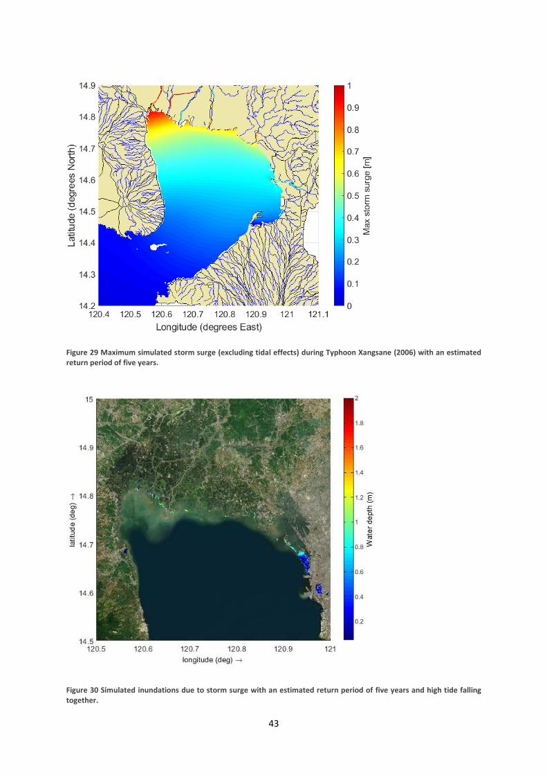
43
Figure 29 Maximum simulated storm surge (excluding tidal effects) during Typhoon Xangsane (2006) with an estimated return period of five years.
Figure 30 Simulated inundations due to storm surge with an estimated return period of five years and high tide falling together.
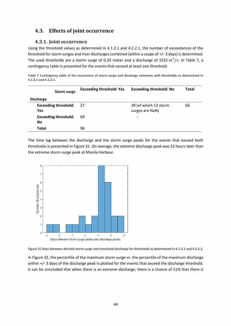
44
4.3. Effects of joint occurrence
4.3.1. Joint occurrence Using the threshold values as determined in 4.1.2.1 and 4.2.2.1, the number of exceedances of the
threshold for storm surges and river discharges combined (within a scope of +/- 3 days) is determined.
The used thresholds are a storm surge of 0.20 meter and a discharge of 1532 𝑚3/𝑠. In Table 7, a
contingency table is presented for the events that exceed at least one threshold.
Table 7 Contingency table of the occurrence of storm surge and discharge extremes with thresholds as determined in 4.1.2.1 and 4.2.2.1.
Storm surge
Discharge
Exceeding threshold: Yes Exceeding threshold: No Total
Exceeding threshold: Yes
27 39 (of which 13 storm surges are NaN)
66
Exceeding threshold: No
69 -
Total 96
The time lag between the discharge and the storm surge peaks for the events that exceed both
thresholds is presented in Figure 31. On average, the extreme discharge peak was 22 hours later than
the extreme storm surge peak at Manila Harbour.
Figure 31 Days between derived storm surge and simulated discharge for thresholds as determined in 4.1.2.1 and 4.2.2.1.
In Figure 32, the percentile of the maximum storm surge vs. the percentile of the maximum discharge
within +/- 3 days of the discharge peak is plotted for the events that exceed the discharge threshold.
It can be concluded that when there is an extreme discharge, there is a chance of 51% that there is

45
also an extreme storm surge within a timeframe of +/- 3 days. When all the timesteps are taken into
account, the chance that a storm surge exceeds the threshold within a timeframe of +/- 3 days is 8.0%.
Figure 32 Percentile-percentile of the storm surge and discharge peaks with the simulated extreme discharges as a starting point and a timeframe of +/-3 days between the storm surge and discharge peaks. The red line is the storm surge threshold.
In Figure 33, the storm surge peaks are used as a starting point. This results in the percentile of the
discharge peak for all the storm surges that exceed the threshold. It can be concluded that when there
is a storm surge, that there is a chance of 28% that there is also an extreme discharge event within a
timeframe of +/- 3 days. When all the timesteps are taken into account, the chance of a discharge that
exceeds the threshold is 5.1%. This significant difference shows that there is a clear dependence
between extreme storm surges and extreme discharges.
Figure 33 Percentile-percentile of the storm surge and discharge peaks with the derived extreme storm surges as a starting point and a timeframe of +/-3 days between the storm surge and discharge peaks. The red line is the discharge threshold.

46
4.3.2. Time lag
4.3.2.1. Storm surge during discharge peaks
In Figure 34, the probability density plot for the storm surge at Manila Harbour at different time lags
before the discharge peak is given. It can be seen that the largest probability of high storm surges
occurs with a time lag of 30-36 hours between the discharge and the storm surge. In Table 8, the
average storm surge for the different time lags is given together with the standard deviation. Based
on Table 8 and Figure 34, it can be concluded that the largest storm surges occur 30-36 hours before
the extreme discharge peaks and that there is a significant increase of the storm surge when there is
an extreme discharge peak.
It can be seen in Figure 34 that the probability density plot differs significantly from the PDF with a
time lag of one year. The storm surge with a time lag of one year has an average of approximately
zero, which means that the increased storm surges cannot be attributed to seasonal behaviour.
Figure 34 Probability Density of the derived storm surges at Manila Harbour with different time lags between the storm surge and discharge peak.

47
Table 8 Average storm surge and standard deviation at Manila Harbour with different time lags after an extreme discharge peak.
Time lag Average storm surge [m] Standard deviation [m]
0 0.051 0.094
6 0.064 0.102
12 0.071 0.099
18 0.086 0.099
24 0.1 0.123
27 0.091 0.132
30 0.112 0.148
33 0.103 0.156
36 0.112 0.138
42 0.062 0.099
48 0.068 0.086
1 year 0.008 0.062
4.3.2.2. Discharge during storm surge peaks
In Figure 35, the probability density plot for the discharge at different time lags after an extreme storm
surge peak is given. In Table 9, the average discharge for the different time lags is given together with
the standard deviation. Based on Table 9, it can be concluded that the peaks of the extreme discharge
event occur approximately 36 hours after the storm surge peak at Manila Harbour. It can be seen in
Figure 35 that the probability density plot differs significantly from the PDF with a time lag of one year.
This means that the increased discharge cannot be attributed to seasonal behaviour only.
Figure 35 Probability density of the discharge at the Pampanga River with different lags between the storm surge and the discharge peak.

48
Table 9 Average discharge and standard deviation after an extreme storm surge peak with different time lags.
Time lag [hours]
Average discharge
[𝒎𝟑/𝒔]
Standard deviation
[𝒎𝟑/𝒔]
0 693 509
6 726 549
12 769 598
18 819 639
24 895 712
27 936 766
30 966 813
33 979 829
36 981 818
39 975 793
42 965 762
48 943 709
1 year 583 472
4.3.3. Inundation simulations in Delft3D-FLOW
4.3.3.1. Simulation of a historical event
The six events (including Typhoon Nesat) that have the highest cumulative percentile (of the maximum
discharge and maximum surge) are given in Table 10. For two typhoons that are mentioned in Table
10, historical flood maps based in satellite images are available. That are Typhoon Nesat 2011
(PRFFWC, 2012) and typhoon Ketsana in 2009 (Brakenridge, 2009). Typhoon Nesat was a typhoon that
tracked in west-north-western direction and caused a damage of 2.12 billion USD. The discharge of
the Pampanga River had an approximated return period of 11 years and the storm surge at Manila
Harbour of 165 years. Typhoon Ketsana tracked in western direction over the Pampanga delta and
resulted in extreme precipitation at Metro Manila. The discharge of the Pampanga River had a return
period of approximately ten years and the storm surge at Manila Harbour had a return period of
approximately five years. The observed inundation extent that is caused by Typhoon Ketsana is
presented in Figure 36.
Table 10 Events with the highest cumulative percentile of derived storm surge and simulated discharge peak.
Date Sum percentiles
Percentile discharge
Discharge
[𝒎𝟑/𝒔]
Percentile surge
Surge [𝒎]
Typhoon Cat
28-Sep-2011 12:00:00 199.99 99.99 3580 100 0.77 Nesat 4
07-Oct-1993 00:00:00 199.97 100 4308 99.97 0.36 Ed 5
27-Sep-2009 09:00:00 199.97 99.98 3492 99.99 0.42 Ketsana 2
26-Oct-1988 06:00:00 199.86 99.86 2543 100 0.65 Ruby 4
02-Oct-1995 09:00:00 199.87 99.92 2893 99.93 0.31 Sibyl 2
13-Oct-2013 00:00:00 199.79 99.81 2409 99.97 0.37 Nari 3

49
Figure 36 Inundation (red parts) based on satellite images due to Typhoon Ketsana in 2009 (Adapted from (Brakenridge, 2009)).

50
The timing of the storm surge, discharge and tide during Typhoon Ketsana is presented in Figure 37.
The peak of the storm surge, tide and discharge do not fall together, which might have a significant
influence on the inundations that occur.
Figure 37 Derived tide, derived storm surge and simulated discharge during Typhoon Ketsana (2009).
The results of the inundations in the Pampanga delta due to Typhoon Ketsana are presented in Figure
38. As can be seen, the results do not fit very well with the measured inundations. Also for Typhoon
Nesat, the simulated inundations do not correspond well with the observed inundations (not shown
here, see PRFFWC (2012)). Partially this difference can be explained by the overestimations of the
discharges, following from the fact that inundations along the river, upstream of the Delft3D-FLOW
model boundaries, are not taken into account. Also, deviations in the simulated discharges itself can
result in differences between the simulated and measured inundations. Furthermore, it might have to
do with the DEM that is used in the Delft3D-FLOW model which has a resolution of 30 meters and
does not include important details like fish ponds and small dykes. Also, the boundaries of the model
are not set properly; the straight line that is visible in the inundation extent has a significant influence
on the simulations and indicates that the upstream boundary conditions are not set in the right
location. Another reason for the differences between the simulated and the measured inundations is
the storm surge generation in Delft3D-FLOW, which was significantly less than the measured storm
surge for Typhoon Ketsana. Investigation of the measured storm track (see Figure 39) and intensity of
Typhoon Ketsana shows that the typhoon was only a very weak tropical storm with a wind speed of
65 km/h and a pressure of 996 mb when it passed Manila. This indicates that the measured water
levels were not caused by Typhoon Ketsana on its own but might be exacerbated by other effects like
the SW Monsoon; an effect that was also visible during Typhoon Nesat (Morin et al., 2016). Since the
monsoon is not incorporated in Delft3D-FLOW this can result in an underestimation of the storm surge.

51
Figure 38 Simulated inundations due to Typhoon Ketsana (2009).
Figure 39 Track of Ketsana (Cyclonebiskit, 2009).
4.3.3.2. Simulation of different scenarios
For the simulations of the different scenarios, a storm surge at Manila Harbour and the discharges
with an estimated return period of five years for the Pampanga River have been used. The storm surge
at Manila Harbour that has a return period of five years is approximately 0.42 cm. The adapted wind
and pressure fields for typhoon Xangsane (2006), as described in section 4.2.3, will be used. The
discharge peak of the Pampanga River that has an estimated return period of five years, corresponding
to the wflow discharges, is approximately 3000 𝑚3/𝑠. Therefore, the discharge waves that were
simulated for Typhoon Xangsane has been scaled to reach a maximum discharge of 3000 𝑚3/𝑠 for the
Pampanga River. Based on this adapted wind and pressure field and the discharges with an estimated
return period of five years, the inundations are simulated for the scenarios that are presented in Table

52
3. The results are presented in Figure 41-49. In Figure 40, the simulated water level at Manila harbour
is given for the different scenarios. The temporal decline of the storm surge that is visible is probably
caused by the centre of the eye that passed directly over Manila Bay.
Figure 40 Simulated water levels with a storm surge with an estimated return period of five years based on different scenarios at Manila Harbour.

53
Figure 41 Simulated inundations scenario 1. Discharge, surge and tide peaks together.
Figure 42 Simulated inundations scenario 2. Discharge and tide peaks together, no surge.
Figure 43 Difference in inundations between scenario 1 and 2.

54
Figure 44 Simulated inundations scenario 3. Discharge and surge peaks together during lowest tide.
Figure 45 Difference in inundations between scenario 1 and 3.
Figure 46 Simulated inundations scenario 4. Discharge peaks during lowest tide, no surge.
Figure 47 Difference in inundations between scenario 1 and 4.

55
Figure 48 Simulated inundations scenario 5. Surge and tide peaks together, no discharge.
Figure 49 Difference in inundations between scenario 1 and 5.
In Figure 46, the inundations due to river discharges only are presented. Based on Figure 47, it can be
concluded that the flood extent is dominated by the discharges. Even without storm surge and with
low tide, the flooded area is almost the same as in Figure 41. Despite the dominance of the discharges
on the flooded area, the water depth of the inundations is increased over a large area due to the joint
occurrence of storm surge, high discharges and high tides. The storm surge and the timing of the storm
surge with respect to the tide have a significant influence in some coastal areas and in the north-
western part of Manila. Without discharges, the joint occurrence of high storm surge and high tide
results locally in inundations as can be seen in Figure 48.
From Figure 43 it can be concluded that neglecting the storm surge during discharge peaks will result
in an underestimation of the inundation depth over a large area. Also, the timing of the storm surge
and discharge peaks with respect to the tide can have a significant influence over a large area (Figure
45) and can have a large influence on a local scale.

56
The effect of the joint occurrence
of the tide, storm surge and
discharges is larger than the sum
of the inundations by the
discharges and the inundations
by the storm surge and tide. This
exacerbated inundations due to
the joint occurrence is presented
in Figure 50.
The simulated discharge with an
estimated return period of five
years is higher than the highest
discharge that is determined
based on the measured water
levels and the highest rating
curve (Van ’t Veld, 2015).
Therefore, the simulated scenarios presented in Figure 41-49 are assumed to be the upper boundary
for the river discharges with an estimated return period of five years. In Appendix A.III., the results for
the simulations based on the highest measured discharge with the lowest rating curve (JICA, 2009) are
presented. These simulations are considered as the lowest discharge boundary. Based on these figures,
it can be concluded that the dominance of the discharges and the small influence of the surge is not
the result of an overestimation of the discharges with an estimated return period of five years. Even
with relative small discharges, the flooding pattern is dominated by the discharges.
In Figure 6, the elevation in the Pampanga delta is presented (based on MERIT-DEM data). The blue
parts are the low lying areas (<1 m). The areas that show the largest influence of the storm surge/tide
during high discharges on the inundations (Figure 47) correspond quite well with the lower parts close
to Manila Bay and the lower parts more upstream in the delta (see also Figure 6). This behaviour is
logical since these areas can be directly flooded by the storm surge. The areas in the north-western
part of the Pampanga delta can be flooded due to storm surge since there are multiple fishponds and
lakes between the flooded area and Manila Bay, which means that the water can flow directly into
these low lying areas (see Figure 5).
Figure 50 Aggravated simulated inundations due to joint occurrence of storm surge, tide and discharge peaks (Scenario1 - (Scenario2 + Scenario5)).

57
5. DISCUSSION
5.1. Potential of this research This study shows that the inundated area due to typhoons in the Pampanga delta is dominated by the
river discharge, although there are locations in the surroundings of Manila Bay and in the north-
western part of Manila, where the storm surge is dominant. This research also gives an understanding
of the time lag between the storm surge and the discharge peaks and shows that the occurrence of
storm surge and discharge peaks cannot be assumed to be independent. Furthermore, this study
shows that it is important to take the storm surge and the timing with respect to the tide into account
in determining the inundation depth over a large area. Taking the discharges as only forcing in
inundation modelling and in risk/exposure studies in the Pampanga delta will result in an
underestimation of the inundations and the risk/exposure.
Multiple studies were conducted on the joint occurrence of storm surges and extreme river discharges.
Those studies focused mainly on the statistical dependence between the storm surge and the
discharge but not on the consequences of the dependence that was found (Svennson & Jones, 2004;
Svensson & Jones, 2002; Zheng et al., 2013). The scarcity of studies on compound flooding due to river
discharge and storm surge is caused by the lack of the ability to present backwater effects in rivers
and the lack of coastal water level data (Ikeuchi et al., 2017). This study uses a method that can
incorporate the backwater effects to simulate compound flooding due to storm surges and discharges.
Chen and Liu (2014) studied the impact on inundations of storm surge only, river discharge only and
the effect of storm surge combined with discharges with an estimated return period of 50, 100 and
200 years in the Tsengwen River basin in Taiwan. The catchments area of this basin is 1177 𝑘𝑚2 which
is significantly smaller than the catchment area for the Pampanga River which is 7978 𝑘𝑚2. The used
storm surge was 3.26 m at the river mouth, while in this research the used storm surge at the river
mouth varies between 0.6 m and 1.0 m. Their results, that compound flooding due to discharge and
storm surge results in exacerbated inundations, are in accordance with the results of this study. The
dominance of the river discharge that was found in this study, was not shown in the study of (Chen &
Liu, 2014). They found a significant increase of the inundations for the compound flooding. But since
we are looking at a different location and a different severity, it is hard to draw firm conclusions based
on this difference.
This study shows the impact of the joint occurrence of storm surge and discharge peaks on the flood
extent and the inundation depth. This approach might be useful for future research in other catchment
areas since it shows the consequences of the joint occurrence of high tides, storm surges and extreme
discharges. The applied approach in the inundation modelling for the different scenarios can also be
applied with other models. A good example is the Super-Fast Inundation of CoastS (SFINCS) model,
that is able to simulate all hydrodynamic processes two orders of magnitude faster than Delft3D-FLOW
with limited deviations (Torres Dueñas, 2018). This model makes it possible to simulate multiple
scenarios within limited time and makes it possible to simulate a wide range of events with different
storm surge and discharge combinations.

58
5.2. Limitations
5.2.1. Data Some conclusions that will be drawn are based on measured data and simulations in wflow and
Delft3D-FLOW. The accuracy of these simulations depends for a large part on the quality of the input
data. For the wflow model, the global MSWEP dataset is used as precipitation input for the model.
This dataset performed better than four other state-of-the-art gauge adjusted precipitation datasets
(Beck et al., 2017). Despite the relatively good performance of this dataset, it is known that global
precipitation data can show large deviations from observations (Covey et al., 2003, 2018).
The comparison of the precipitation during Typhoon Nesat (2011) and Typhoon Utor (2013) showed
a total precipitation amount that corresponds quite well with the measured precipitation. This may
be promising but needs further validation by using the data set for other typhoons. Furthermore,
deviations in the timing of the MSWEP data might have an influence on the conclusions that will be
drawn about the coincidence. Also, the pattern and amount of the MSWEP precipitation play an
important role in the accuracy of the simulated discharges. The pattern, amount and timing of the
potential evapotranspiration can also differ from the real potential evapotranspiration and can,
therefore, have a significant influence on the wflow simulation. Nevertheless, the accuracy of the
potential evapotranspiration will have a smaller influence than the accuracy of the precipitation, since
the variations in the potential evapotranspiration are a lot smaller and are less important for the
timing and amount of the peak discharges.
The accuracy of the measured water levels is very important in the calibration of the wflow model.
The measured water levels contain a lot of gaps during typhoons due to different reasons. This results
in less measured peak discharges which makes it harder to calibrate and validate the model for a
period of several years. Also, the used rating curves are both very unreliable. JICA (2011) derived rating
curves that seem to underestimate the discharges in multiple rivers. Furthermore, they derived rating
curves (including boundary conditions) for locations that are influenced by the tide. Using rating
curves at locations so far downstream does not make sense and is not useful in determining discharges.
The measured water levels at Manila Harbour that are used to derive storm surges contain, besides
the storm surges due to typhoons and tide, also other influences. Morin et al. (2016) showed that
during the southwest monsoon, water levels at Manila Bay’s Harbour can increase with 20 cm. So, the
values that are presented in section 4.2 as storm surges due to typhoons, are influenced by some
external factors as well.
The used best track files that are derived by the JTWC are estimates of the cyclone’s track and intensity
during the lifetime of the typhoon. The best track files are temporally inhomogeneous due to the
available data and an increase of knowledge about determining the wind and pressure fields (Knapp
& Kruk, 2010). A lowering of 30% in the wind speed can result in a lowering of the storm surge of 70%
(Vatvani, 2018). Also, the track of a typhoon and the radius of maximum wind are very important.
Deviations of 20 km in the track of a typhoon can have a significant influence on the storm surge that
occurs in the simulation. Furthermore, the best track differs at each agency that provides the best
track data due to different procedures (Knapp & Kruk, 2010). The used best track data is therefore
uncertain and can result in different results.

59
5.2.2. Wflow model The wflow model that is used in this research does not perform well and the results of the hydrological
simulations are not very reliable. This has mainly to do with the used catchment area and the absence
of the right static maps (e.g. land use and soil layer maps). As described in section 2.4.1, the model
contains a larger catchment area (10-15%) than in reality. The increased catchment results in higher
discharges but also in a possible time shift of the discharge peaks, which influences the analyses of the
time lag between the storm surges at Manila Harbour and the discharges in the Pampanga River and
might influence the inundation maps that are made in Delft3D-FLOW. Since the erroneous parts of
the catchments are far upstream, the discharge peaks might arrive a bit later, resulting in a larger lag
between the discharge and storm surge peaks. The inaccuracies in the DEM that is used and the
subsequent errors in the local drainage direction are a strong indication that the locations of the rivers
in wflow are not completely in the right position. If the rivers were all at the right location, the error
in the catchment area was not there as well. The model discharges to the right location, but the river
routing more upstream might have changed the discharge time series.
The measured water levels contain a lot of gaps, which made it hard to find a long period that is useful
for the calibration. The period of one year that is chosen to use in the calibration and in the validation
did not contain gaps but using relative short periods of one year reduces the accuracy of the
calibration and validation since fewer extreme events are considered. Also, the absence of the static
maps, made it very hard to calibrate the model. Normally the calibration occurs by changing e.g. the
depth of some soil layers, but due to the uniform values of the static maps, this was not possible. Also
the sensitivity analysis that is used to select the parameters that have to be calibrated is influenced by
the absence of static maps and is therefore only useful for the used model and is not reliable for future
research. In combination with the uncertainty in the rating curves, the unreliable wflow model results
in a very uncertain discharge time series, both in timing and volume of the discharge peaks. This
uncertainty might have a significant effect on the conclusions that will be drawn.
The rating curve at mount Arayat is taken as reference for the Pampanga River and the calibration of
the whole model has been conducted based on this rating curve. This means that the calibration for
other rivers in the wflow model was also conducted by changing the same parameter values. This was
the only option since there were no reliable rating curves available for the other rivers, but it makes
the calibration of the whole model less reliable. The uncertainty in the used data, as described in
section 5.2.1, can have a significant influence on the timing of the simulated discharge peaks. The
timing is important in calculating the time lag and in determining the effect of the joint occurrence by
the inundation simulations. Also the absence of the storage dams in the wflow model will have an
influence on the severity and timing of the discharge peaks by storing some of the run-off from the
mountainous areas. The active storage capacity (e.g. 2.1*109 m3 for the Pantabangan dam) is large
enough to store the discharge wave of the Pampanga River during typhoons with an estimated return
period of five years. The location of the Pantabangan storage dam is the limiting factor since
approximately 10% of the Pampanga catchment area lies upstream of this dam.
Despite all the uncertainties, the wflow model was of major importance in this study. The model gives
insight into the magnitude of the lag between the discharge and surge peaks. Furthermore, the wflow
model gives insight in the discharges during typhoons, which cannot be done based on the water level
measurements due to failures of the water level measurement stations during typhoons. Determining
the discharge during extreme events was necessary to estimate the discharge with an estimated

60
return period of five years that is used in the inundation simulations of the different scenarios. It can
be concluded that there are some serious issues regarding the reliability of the wflow model, but at
the same time, the model plays an essential and indispensable role in this study.
5.2.3. Delft3D-FLOW model The Delft3D-FLOW model uses wind and pressure fields as forcing data. Inaccuracies in the wind and
pressure fields and in the track of the typhoon can result in significant deviations of the storm surge,
which will have an influence on the simulated inundations. The impact of inaccuracies in the forcing
data on the inundation maps is minimized since the spiderweb file has been adapted to reach a storm
surge with approximately a return period of five years at Manila Harbour. Also, the DEM has a major
influence on the inundations. The used DEM is the SRTM30 DEM with a resolution of 1 arc-second. It
is already known that the used DEM in this model does not show all the small dikes and fish ponds in
the Pampanga delta, which has a significant influence on the inundations (Vatvani, 2016). The vertical
accuracy of the SRTM30 DEM in the Philippines (measured in the mountainous areas of North-eastern
Mindanao) is limited since it has a RMSE of 8.3 meters (Santillan & Makinano-Santillan, 2016). The
accuracy in the Pampanga delta is probably better but using the SRTM30 DEM for inundation
simulations is very doubtful. Even though Vatvani (2016) adapted the SRTM DEM in the Delft3D-FLOW
model, inaccuracies in the inundations will occur. Using a more accurate DEM, e.g. the 10-meter
resolution Lidar DEM which has a vertical accuracy of 15 cm in open areas (Reutebuch et al., 2003),
will increase the accuracy of the results significantly.
Different studies (Morin et al., 2016; Raucoules et al., 2013) and Figure 20 show that relative sea level
rise, mainly caused by land subsidence, will play a major role in determining inundations in Metro
Manila. With extraordinary rates of the current subsidence (up to 45 mm/year (Eco et al., 2011)) this
forms a large threat to Manila. If the current subsidence continues, Metro Manila subsides within a
decade more than a storm surge with an estimated return period of five years. This also means that
the results of this study will be temporal and that the influence of storm surges will increase in the
future.
In the simulated inundations, the model boundary is clearly visible. This indicates that the model
results are influenced by the boundaries and that the boundaries are too far downstream. Also, the
locations of the river input in the model are too far downstream, since they are modelled at a location
where already inundations occur. This has a significant influence on the modelled inundations. Further,
more upstream of the wflow input in the Delft3D-FLOW model there are already inundations along
the river. These inundations will flatten the discharge peaks and therefore results in lower inundations
downstream. In the simulations, this effect is not considered which results in an overestimation of the
discharge input at the rivers and, subsequently, an overestimation of the inundations and impact of
the river discharges in the Pampanga delta.
Morin et al. (2016) showed that it was neither the most intense nor the closest typhoon that resulted
in the largest storm surges in Manila Bay. This indicates that the storm surge is influenced by a wide
range of other factors and that using only the wind and pressure fields in simulating the storm surges
in Manila Bay, results in a deviation from the actual storm surge.

61
5.3. Challenges
5.3.1. Data quality Improving the amount, timing and distribution of the MSWEP data to make sure that it is a reliable
source for the simulation of historical typhoons is a challenge. This can be done by comparing the total
amount of precipitation, the precipitation during typhoons and the timing of the precipitation peaks
with measured precipitation data. This will require a significant amount of time if this needs to be
done manually, but machine learning techniques might be able to improve the data automatically.
Local measurements of the evapotranspiration can be used to improve the potential
evapotranspiration data in the same manner.
Measured discharges or water levels with reliable rating curves are of major importance for the
calibration of the hydrological model. Therefore, taking new measurements of the discharges and
water levels is required. During the measurements, extra attention is required during extreme events
to retrieve data without gaps. Also, measurements of the typhoons windspeed, pressure field and
location are required to calibrate the JTWC best track data. This data plays a significant role in the
storm surge generation and needs to be reliable, but doing measurements during extreme events will
be a major challenge due to the life-threatening circumstances that can occur.
5.3.2. Wflow model A new wflow model needs to be developed. When making this model, extra attention is required for
the river routing to prevent inaccuracies in the local drainage direction and the used catchment area.
In this model, new static maps need to be incorporated to come up with a model that have a good
approximation of the land use and soil layers. To do so, global datasets are available but validation
with local data is necessary. Also taking into account the storage dams, spillway capacity and reservoir
operation is important. The model needs to be calibrated and validated for different rivers, based on
(reliable) discharge measurements or water level measurements and rating curves. Making a wflow
model is relatively easy with the modelbuilder. The modelbuilder is a tool developed by Deltares, that
uses global datasets to make a wflow model. During this research, there were problems with the
modelbuilder that made it impossible to make a new model, but it should be fixed nowadays.
5.3.3. Delft3D-FLOW model Also, a new Delft3D-FLOW model needs to be developed. It is important that a more accurate DEM is
used that incorporates small dikes and fishponds in the Pampanga delta. This DEM should be up-to-
date, to incorporate recent land subsidence as well. The model boundaries and upstream discharge
boundary conditions need to be located more upstream, in such a way that the model boundaries do
not influence the inundations that occur in the Pampanga delta. To do so, an integrated approach with
a good collaboration of different experts is required. To prevent that the hydrological model and the
hydrodynamic model are developed separately and are not merged in an optimal way, you need to
involve people with expertise in both disciplines.
In Delft3D-FLOW, more processes need to be added in order to come up with more reliable storm
surge simulations. Morin et al. (2016) showed that storm surge in Manila Bay is influenced by a wide
range of other factors (like the southwest monsoon winds) and that using only the wind and pressure
fields in simulating the storm surges in Manila Bay results in a deviation from the actual storm surges.

62
6. CONCLUSIONS
6.1. Conclusions on the effect of typhoons on discharges and
subsequent inundations in the Pampanga delta Based on simulations with the hydrological wflow model, it can be concluded that typhoons can result
in extreme discharges in the Pampanga delta. All the ten highest simulated discharge peaks of the
Pampanga River, are the result of tropical storms and typhoons. On average, two discharge peaks per
year exceed the threshold of 1532 𝑚3/𝑠. Based on a Generalized Pareto Distribution fit the estimated
return period of the discharge peaks is determined. It follows that the discharge in the Pampanga River
with an estimated return period of five years is approximately 3000 𝑚3/𝑠. This discharge of 3000
𝑚3/𝑠 results in severe simulated inundations over a large area in the Pampanga delta. The inundation
depth reaches values up to 2 meters, with the deepest parts around the river inflow point of the
Pampanga main river.
6.2. Conclusions on the effect of typhoons on storm surges in
Manila Bay and subsequent inundations in the Pampanga
delta Based on water level measurements in Manila Bay, harmonic analysis with the MATLAB toolbox T_Tide
and corrections for sea level rise and subsidence, the storm surges in Manila Bay are derived. Nine out
of the ten highest storm surges at Manila Harbour are the result of a typhoon or tropical storm. Using
a Generalized Pareto Distribution fit on the storm surge peaks results in a storm surge at Manila
Harbour with an estimated return period of five years of 42 cm. Which is relatively small in comparison
with the tidal influence that varies between approximately -1.0 m and +1.0 m. Simulations in Delft3D-
FLOW show that there is a significant variation of the storm surge over Manila Bay, with the highest
storm surge values occurring in the northern part of Manila Bay. When the peak of the storm surge
with an estimated return period of five years falls together with high tide in Manila Bay, this results in
inundations on a local scale in north-western Manila and in areas in the surroundings of Manila Bay.
But the inundation extent induced by the storm surge is small in comparison with the inundation
extent induced by the river discharge with an estimated return period of five years. Due to sea level
rise and land subsidence, which has an average rate of 45 mm/year in Metro Manila, the importance
of storm surge in exposure and risk studies in the surroundings of Manila Bay will increase rapidly in
the future.
6.3. Conclusions on the effect of joint occurrence of storm surges
and discharge peaks on inundations in the Pampanga delta From the 66 discharge events that exceed the threshold value of 1532 𝑚3/𝑠, 27 discharges occurred
within a period of three days before or after an extreme storm surge event at Manila Harbour that
exceeds the threshold of 20 cm, 26 do not fall together with an extreme storm surge within three days
before or after, and during 13 discharges the storm surge is not measured. The average time lag
between the storm surge and discharge peaks is 36 hours and the average time lag seems to decrease
to 22 hours for events where both peaks are extreme. Also, without a time lag between the storm
surge and discharge peaks, there is an increased probability of higher storm surge levels in comparison
with the independent probability, which means that the storm surges and the discharges are not
independent.
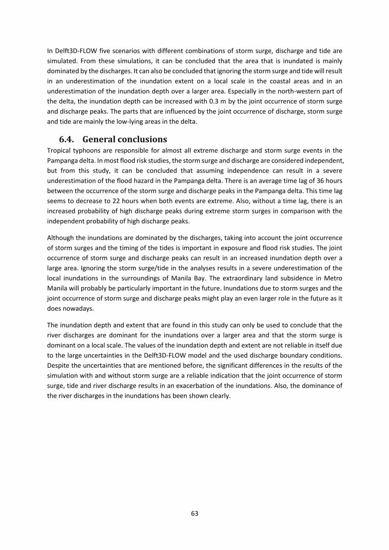
63
In Delft3D-FLOW five scenarios with different combinations of storm surge, discharge and tide are
simulated. From these simulations, it can be concluded that the area that is inundated is mainly
dominated by the discharges. It can also be concluded that ignoring the storm surge and tide will result
in an underestimation of the inundation extent on a local scale in the coastal areas and in an
underestimation of the inundation depth over a larger area. Especially in the north-western part of
the delta, the inundation depth can be increased with 0.3 m by the joint occurrence of storm surge
and discharge peaks. The parts that are influenced by the joint occurrence of discharge, storm surge
and tide are mainly the low-lying areas in the delta.
6.4. General conclusions Tropical typhoons are responsible for almost all extreme discharge and storm surge events in the
Pampanga delta. In most flood risk studies, the storm surge and discharge are considered independent,
but from this study, it can be concluded that assuming independence can result in a severe
underestimation of the flood hazard in the Pampanga delta. There is an average time lag of 36 hours
between the occurrence of the storm surge and discharge peaks in the Pampanga delta. This time lag
seems to decrease to 22 hours when both events are extreme. Also, without a time lag, there is an
increased probability of high discharge peaks during extreme storm surges in comparison with the
independent probability of high discharge peaks.
Although the inundations are dominated by the discharges, taking into account the joint occurrence
of storm surges and the timing of the tides is important in exposure and flood risk studies. The joint
occurrence of storm surge and discharge peaks can result in an increased inundation depth over a
large area. Ignoring the storm surge/tide in the analyses results in a severe underestimation of the
local inundations in the surroundings of Manila Bay. The extraordinary land subsidence in Metro
Manila will probably be particularly important in the future. Inundations due to storm surges and the
joint occurrence of storm surge and discharge peaks might play an even larger role in the future as it
does nowadays.
The inundation depth and extent that are found in this study can only be used to conclude that the
river discharges are dominant for the inundations over a larger area and that the storm surge is
dominant on a local scale. The values of the inundation depth and extent are not reliable in itself due
to the large uncertainties in the Delft3D-FLOW model and the used discharge boundary conditions.
Despite the uncertainties that are mentioned before, the significant differences in the results of the
simulation with and without storm surge are a reliable indication that the joint occurrence of storm
surge, tide and river discharge results in an exacerbation of the inundations. Also, the dominance of
the river discharges in the inundations has been shown clearly.
64
7. RECOMMENDATIONS Based on the discussion and conclusions, some recommendations are formulated for further research
and for policymakers and water managers in the Pampanga delta.
7.1. Recommendations for further research First, further research in the Pampanga delta urgently needs better water level and discharge data.
Reliable water level measurements and discharges are required to derive reliable rating curves in the
Pampanga delta. These rating curves can be used to derive discharges based on the time series of
measured water levels.
Second, precipitation measurements should be taken at more measurement stations over the area.
These measurements can be used to improve the MSWEP data or other forcing data, especially for
the precipitation during typhoons. Improving the forcing data for the hydrological model is a major
step to improve the reliability of the simulated discharges.
Third, a new wflow model should be made that incorporates the correct catchment area, the correct
rivers, storage dams and their spillway capacity and reliable static maps (e.g. soil layers and land use).
The model can be calibrated based on the time series with discharge measurements. Before
calibrating, a sensitivity analysis of the different model parameters should be conducted, since the
sensitivity analysis that had been conducted in this research cannot be used for the new model.
Fourth, the annual potential evapotranspiration in the Pampanga delta is in the order of 50% of the
annual precipitation and therefore has a significant influence on the discharge and the conditions prior
to a typhoon’s arrival. It is interesting to investigate the effect of the potential evapotranspiration on
the discharge during typhoons to produce a more reliable discharge simulation, this might be done
with a sensitivity analysis.
Fifth, it would be interesting to investigate the reasons for the over-/underestimation of the storm
surge for Typhoon Ketsana and Typhoon Xangsane in Delft3D-FLOW. Are the best track data, derived
from the JTWC, reliable? Do the wind and pressure fields correspond with measured data? Is the used
bathymetry of Manila Bay of a decent quality? It is also interesting to investigate the impact of the
used DEM on the inundation extent of the different scenarios.
Sixth, when more reliable hydrological (wflow) and hydrodynamic (Delft3D-FLOW) models are
available, it would be interesting to investigate several factors that influence the probability of joint
occurrence of storm surge and discharge peaks. Factors that can be incorporated in such research are
e.g. the distance of the typhoon track to Manila Bay, the typhoon strength and the angle of approach
of the typhoon. This can eventually be done with synthetic generated typhoon data that can be
changed in a systematic manner.
Seventh, it would be interesting to quantify the hazard related to the joint occurrence of storm surges
and high discharges. Interesting questions are how many people and houses are affected by the
inundations and which important infrastructure is affected. These questions can be used in evacuation
and emergency plans. Another research can be to investigate the risk related to the joint occurrence,
for example with Delft FIAT (Flood Impact Assessment Tool). Therefore, damage functions should be
determined that couple the water depth with object maps and maximum damage. In this way, damage
maps can be made that can be used to protect the most important areas.

65
Last, it would be interesting to investigate the effect of (future) land subsidence and sea level rise on
the joint occurrence of storm surge and discharge peaks and on the inundations in the surroundings
of Manila Bay. With the existing land subsidence and sea level rise, the impact of the storm surges will
increase rapidly in the future, resulting in more severe inundations and larger problems.
7.2. Recommendations for policy makers and water managers Based on the results of this study, some recommendations are given to policy makers and water
managers in the Pampanga delta.
First of all, this study shows that the joint occurrence of storm surges, high tides and extreme
discharges results in an exacerbation of the inundations that will occur. Increasing the time lag
between the surges and the discharges is a good option to mitigate the inundations. This can be done
by measures that hold the water upstream for a longer period. Reservoirs might be able to increase
the time lag between the discharge and storm surge peaks; reservoir operation and forecasting will
play a crucial role in this process. The same reservoirs can also be used to reduce the discharge peaks
itself by flattening the discharge peaks of extreme events. Lowering the discharge peaks will mitigate
the inundations in the Pampanga delta.
Second, this research shows that high river discharges can result in severe inundations over a large
area. Increasing the discharge capacity is necessary to prevent future inundations due to severe
precipitation and discharges in the Pampanga delta.
Last, storm surge barriers can prevent inundations due to storm surges on a local scale in the areas in
the surroundings of Manila Bay and in the north-western part of Metro Manila. The highest surges
occur in the north and especially north-western part of Manila Bay. Due to the extraordinary
subsidence in Metro Manila, taking into account storm surges in this area will probably be more
important in the future than it is nowadays.

66
8. BIBLIOGRAPHY Ahmad, I., Verma, V., & Verma, M. K. (2015). Application of Curve Number Method for Estimation of
Runoff Potential in GIS Environment. IPCBEE, 80(4). https://doi.org/10.7763/IPCBEE
Beck, H. E., Van Dijk, A. I. J. M., Levizzani, V., Schellekens, J., Gonzalez Miralles, D., Martens, B., & De Roo, A. (2017). MSWEP: 3-hourly 0.25 global gridded precipitation (1979-2015) by merging gauge, satellite, and reanalysis data. Hydrology and Earth System Sciences, 21(1), 589–615.
Bernardara, P., Mazas, F., Kergadallan, X., & Hamm, L. (2014). A two-step framework for over-threshold modelling of environmental extremes. Natural Hazards and Earth System Sciences. https://doi.org/10.5194/nhess-14-635-2014
Bezak, N., Brilly, M., & Šraj, M. (2014). Comparison between the peaks-over-threshold method and the annual maximum method for flood frequency analysis. Hydrological Sciences Journal. https://doi.org/10.1080/02626667.2013.831174
Boccalon, A., Goorden, N., Vernimmen, R., & Schellekens, J. (2014). Use of global datasets for hydro-meteorological analysis in areas with sparse data. Instruction Manual and Exercises.
Booij, M. J., & Krol, M. S. (2010). Balance between calibration objectives in a conceptual hydrological model. Hydrological Sciences Journal–Journal Des Sciences Hydrologiques, 55(6), 1017–1032.
Borges, P. de A., Franke, J., da Anunciação, Y. M. T., Weiss, H., & Bernhofer, C. (2016). Comparison of spatial interpolation methods for the estimation of precipitation distribution in Distrito Federal, Brazil. Theoretical and Applied Climatology, 123(1), 335–348. https://doi.org/10.1007/s00704-014-1359-9
Brakenridge, R. (2009). Dartmouth Flood Observatory. Retrieved September 1, 2018, from http://www.dartmouth.edu/~floods/hydrography/E120N20.ppt
Chen, W.-B., & Liu, W.-C. (2014). Modeling flood inundation induced by river flow and storm surges over a river basin. Water, 6(10), 3182–3199.
Covey, C., AchutaRao, K. M., Cubasch, U., Jones, P., Lambert, S. J., Mann, M. E., … Taylor, K. E. (2003). An overview of results from the Coupled Model Intercomparison Project. Global and Planetary Change, 37(1–2), 103–133.
Covey, C., Doutriaux, C., Gleckler, P. J., Taylor, K. E., Trenberth, K. E., & Zhang, Y. (2018). High Frequency Intermittency in Observed and Model‐simulated Precipitation. Geophysical Research Letters.
De Vos, J., Hamer, F. W., Diederen, D., & Zoric, A. (2014). Manila Bay Delta Challenge - Multidisciplinary Research on Flood Prone Areas in the Pampanga Delta.
Ebrahimian, M., Nuruddin, A. A., Soom, M. A. B. M., & Sood, A. M. (2012). Application of NRCS-curve number method for runoff estimation in a mountainous watershed. Caspian Journal of Environmental Sciences Caspian J. Env. Sci. Printed in I.R. Iran [Research.
Eco, R., Lagmay, A. M., & Bato, M. G. (2011). Investigating ground deformation and subsidence in northern Metro Manila, Philippines using Persistent Scatterer Interferometric Synthetic Aperture Radar (PSInSAR). AGU Fall Meeting Abstracts, 0822-.
England Jr., J. F., Cohn, T. A., Faber, B. A., Stedinger, J. R., Thomas Jr., W. O., Veilleux, A. G., … Mason

67
Jr., R. R. (2018). Guidelines for determining flood flow frequency—Bulletin 17C. Techniques and Methods. https://doi.org/10.3133/tm4B5
Grinsted, A. (2014). Tidal fitting toolbox. Retrieved from https://nl.mathworks.com/matlabcentral/fileexchange/19099-tidal-fitting-toolbox
Ikeuchi, H., Hirabayashi, Y., Yamazaki, D., Muis, S., Ward, P. J., Winsemius, H. C., … Kanae, S. (2017). Compound simulation of fluvial floods and storm surges in a global coupled river‐coast flood model: Model development and its application to 2007 C yclone S idr in B angladesh. Journal of Advances in Modeling Earth Systems, 9(4), 1847–1862.
IPCC. (2012). Managing the risks of extreme events and disasters to advance climate change adaptation. Retrieved from https://www.ipcc.ch/pdf/special-reports/srex/SREX_Full_Report.pdf
Jamandre, C. A., & Narisma, G. T. (2013). Spatio-temporal validation of satellite-based rainfall estimates in the Philippines. Atmospheric Research. https://doi.org/10.1016/j.atmosres.2012.06.024
Jaranilla-Sanchez, P. A., Wang, L., & Koike, T. (2011). Modeling the hydrologic responses of the Pampanga River basin, Philippines: A quantitative approach for identifying droughts TT -. Water Resources Research TA -, 47(3). https://doi.org/10.1029/2010WR009702 LK - https://ut.on.worldcat.org/oclc/5155397263
JICA. (2009). Rating curves.
JICA. (2011). The study on integrated water resources management for poverty alleviation and economic development in the Pampanga River Basin in the Republic of the Philippines. Retrieved from http://www.nwrb.gov.ph/images/Publications/IWRM_Pampanga_River_Basin.pdf
JTWC. (2018). Western North Pacific Ocean Best Track Data. Retrieved from http://www.metoc.navy.mil/jtwc/jtwc.html?western-pacific
Karim, M. F., & Mimura, N. (2008). Impacts of climate change and sea-level rise on cyclonic storm surge floods in Bangladesh. Global Environmental Change, 18(3), 490–500.
Klerk, W. J., Winsemius, H. C., Verseveld, W. J. van, Bakker, A. M. R., & Diermanse, F. L. M. (2015). The co-incidence of storm surges and extreme discharges within the Rhine-Meuse Delta TT -. Environmental Research Letters TA -, 10(3). https://doi.org/10.1088/1748-9326/10/3/035005 LK - https://ut.on.worldcat.org/oclc/5807788298
Knapp, K. R., & Kruk, M. C. (2010). Quantifying interagency differences in tropical cyclone best-track wind speed estimates. Monthly Weather Review, 138(4), 1459–1473.
Lang, M., Ouarda, T. B. M. J., & Bobée, B. (1999). Towards operational guidelines for over-threshold modeling. Journal of Hydrology. https://doi.org/10.1016/S0022-1694(99)00167-5
Lapidez, J. P., Tablazon, J., Dasallas, L., Gonzalo, L. A., Cabacaba, K. M., Ramos, M. M. A., … Malano, V. (2015). Identification of storm surge vulnerable areas in the Philippines through the simulation of Typhoon Haiyan-induced storm surge levels over historical storm tracks. Natural Hazards & Earth System Sciences Discussions, 3(2).
Leadbetter, M. R. (1991). On a basis for “Peaks over Threshold” modeling. Statistics and Probability Letters. https://doi.org/10.1016/0167-7152(91)90107-3

68
Morin, V. M., Warnitchai, P., & Weesakul, S. (2016). Storm surge hazard in Manila Bay: Typhoon Nesat (Pedring) and the SW monsoon. Natural Hazards, 81(3), 1569–1588. https://doi.org/10.1007/s11069-016-2146-y
Muto, M. (2012). 2 Impacts of Climate Change upon Asian Coastal Areas: The Case of Metro Manila. In Climate Change Adaptation and International Development (pp. 91–110). Routledge.
NASA. (2011). Typhoon Nesat. Retrieved from https://earthobservatory.nasa.gov/images/52308/typhoon-nesat
NOAA. (2018). Harmonic Constituents. Retrieved from https://tidesandcurrents.noaa.gov/harcon.html?id=9455732
Pawlowicz, R., Beardsley, B., & Lentz, S. (2002). Classical tidal harmonic analysis including error estimates in MATLAB using TDE. Computers and Geosciences. https://doi.org/10.1016/S0098-3004(02)00013-4
Perez, R. T., Feir, R. B., Carandang, E., & Gonzalez, E. B. (1996). Potential impacts of sea level rise on the coastal resources of Manila Bay: A preliminary vulnerability assessment. Water, Air, and Soil Pollution, 92(1), 137–147. https://doi.org/10.1007/BF00175560
Petroliagkis, T. I., Voukouvalas, E., Disperati, J., & Bildot, J. (2016). Joint Probabilities of Storm Surge, Significant Wave Height and River Discharge Components of Coastal Flooding Event. https://doi.org/10.2788/677778.
PRFFWC. (2012). Post-Flood report 2011-2. Retrieved from http://prffwc.synthasite.com/resources/PRB flood-Sept2011-Pedring-Quiel.pdf
PRFFWC. (2016). Pampanga River Basin Flood Events 2015. Retrieved from http://prffwc.synthasite.com/resources/PRB flood-2015-Lando-Nona.pdf
PRFFWC. (2018). Dataset with measured water levels and rainfall at different locations in the Pampanga river basin (2009-2016).
Raucoules, D., Le Cozannet, G., Wöppelmann, G., de Michele, M., Gravelle, M., Daag, A., & Marcos, M. (2013). High nonlinear urban ground motion in Manila (Philippines) from 1993 to 2010 observed by DInSAR: Implications for sea-level measurement TT -. Remote Sensing of Environment TA -, 139, 386–397. https://doi.org/10.1016/j.rse.2013.08.021 LK - https://ut.on.worldcat.org/oclc/5147655653
Reutebuch, S. E., McGaughey, R. J., Andersen, H.-E., & Carson, W. W. (2003). Accuracy of a high-resolution lidar terrain model under a conifer forest canopy. Canadian Journal of Remote Sensing, 29(5), 527–535.
Reza Asgari, H., Ghiami Bajgirani, A., Pourshahabi, S., & Asgari, B. (2012). Extraction of threshold for partial duration series (case study: Mashhad, Iran).
Ribberink, J. S., de Vriend, H. J., Hulscher, S. J. M. H., & Souren, A.W.M.G. Vermeulen, B. (2016). River dynamics – Shwallow water flows.
Roth, M., Jongbloed, G., & Buishand, T. A. (2016). Threshold selection for regional peaks-over-threshold data. Journal of Applied Statistics, 43(7), 1291–1309. https://doi.org/10.1080/02664763.2015.1100589
Samuels, P. G. (1989). Backwater lengths in rivers. Proceedings of the Institution of Civil Engineers.

69
Santillan, J. R., & Makinano-Santillan, M. (2016). VERTICAL ACCURACY ASSESSMENT OF 30-M RESOLUTION ALOS, ASTER, AND SRTM GLOBAL DEMS OVER NORTHEASTERN MINDANAO, PHILIPPINES. International Archives of the Photogrammetry, Remote Sensing & Spatial Information Sciences, 41.
Satheeshkumar, S., Venkateswaran, S., & Kannan, R. (2017). Rainfall–runoff estimation using SCS–CN and GIS approach in the Pappiredipatti watershed of the Vaniyar sub basin, South India. Modeling Earth Systems and Environment. https://doi.org/10.1007/s40808-017-0301-4
Schellekens, J. (2018). wflow Documentation. Retrieved from https://media.readthedocs.org/pdf/wflow/latest/wflow.pdf
Sperna Weiland, F., Lopez, P., van Dijk, A., & Schellekens, J. (2015). Global high-resolution reference potential evaporation. In 21st International Congress on Modelling and Simulation.
Svennson, C., & Jones, D. A. (2004). Dependence between sea surge, river flow and precipitation in south and west Britain TT -. HYDROLOGY AND EARTH SYSTEM SCIENCES TA -, 8(5), 973–992.
Svensson, C., & Jones, D. A. (2002). Dependence between extreme sea surge, river flow and precipitation in eastern Britain. International Journal of Climatology, 22(10), 1149–1168. https://doi.org/10.1002/joc.794
Tablazon, J., Caro, C. V, Lagmay, A. M. F., Briones, J. B. L., Dasallas, L., Lapidez, J. P., … Malano, V. (2015). Probabilistic storm surge inundation maps for Metro Manila based on Philippine public storm warning signals TT -. Natural Hazards and Earth System Sciences. https://doi.org/10.5194/nhess-15-557-2015 LK - https://ut.on.worldcat.org/oclc/7181433597
Tallaksen, L. M., & Van Lanen, H. A. J. (2004). Hydrological drought: processes and estimation methods for streamflow and groundwater (Vol. 48). Elsevier.
Torres Dueñas, L. (2018). Flood Risk Assessment of the Clear Creek Watershed considering compound events. Retrieved from uuid:3d2791c1-902f-4107-a5ed-2bb41d4de592
TRMM. (2011). TRMM (TMPA) Rainfall Estimate L3 3 hour 0.25 degree x 0.25 degree V7, Greenbelt, MD, Goddard Earth Sciences Data and Information Services Center (GES DISC). TRMM_3B42_7. Html. Retrieved from 10.5067/TRMM/TMPA/3H/7
UHSLC. (2018). Dataset: UH Sea Level Center (UHSLC) Tide Gauge Data (“Quality”): Hourly Data/Manila. Retrieved from http://uhslc.soest.hawaii.edu/thredds/uhslc_quality_hourly.html?dataset=RQH370B
UP TCAGP. (2015). Flood Forecasting and Flood Hazard Mapping for Pampanga River Basin, Disaster Risk Exposure and Assessment for Mitigation (DREAM). Retrieved from https://dream.upd.edu.ph/assets/Publications/UP-DREAM-River-Reports/FMC/DREAM-Flood-Forecasting-and-Flood-Hazard-Mapping-for-Pampanga-River-Basin.pdf
Van ’t Veld, A. (2015). Potential measures to reduce fluvial and tidal floods in the Pampanga Delta.
Vatvani, D. (2016). Storm surge model for joint flood occurrence study.
Vatvani, D. (2018). Personal communication.
Verlaan, M. (2018). Dataset storm surge.
Vertessy, R., & Elsenbeer, H. (1999). Distributed modeling of storm flow generation in an Amazonian rain forest catchment: Effects of model parameterization TT -. Water Resources Research TA -,

70
35(7), 2173–2187. https://doi.org/10.1029/1999WR900051 LK - https://ut.on.worldcat.org/oclc/5156447512
Westra, S. (2018). Australian rainfall & runoff revision projects. Project 18: interaction of coastal processes and severe weather events. Retrieved from http://arr.ga.gov.au/__data/assets/pdf_file/0018/40527/ARR_Project18_Stage2_Report_Final.pdf
Wolanski, E., & Elliott, M. (2016). Estuarine water circulation. Estuarine Ecohydrology, 35–76. https://doi.org/10.1016/B978-0-444-63398-9.00002-7
Zheng, F., Westra, S., Leonard, M., & Sisson, S. A. (2014). Modeling dependence between extreme rainfall and storm surge to estimate coastal flooding risk TT -. Water Resources Research TA -, 50(3), 2050–2071. https://doi.org/10.1002/2013WR014616 LK - https://ut.on.worldcat.org/oclc/5568658763
Zheng, F., Westra, S., & Sisson, S. A. (2013). Quantifying the dependence between extreme rainfall and storm surge in the coastal zone TT -. Journal of Hydrology TA -, 505, 172–187. https://doi.org/10.1016/j.jhydrol.2013.09.054 LK - https://ut.on.worldcat.org/oclc/5162975199
Zijl, F. (2018). Personal communication.

71
A. APPENDIX
A.I. Selecting input data for the wflow simulations
A.I.1. Method First, the method to select the precipitation (section A.I.1.1) and the potential evaporation (section
A.I.1.2) will be described.
A.I.1.1. Precipitation
The measured precipitation data of the PRFFWC (2018) is most reliable to use as forcing.
Unfortunately, this dataset is only available from February 2009 until December 2016 and contains a
lot of gaps. The short period with precipitation data will probably result in too few discharge events
for reliable statistical analyses. Furthermore, the periods for which there is no precipitation available
will have a significant influence on the discharge at periods wherefore precipitation is available. Gaps
in the precipitation prior to the discharge peak will result in a higher saturation deficit and therefore
influence the amount of direct runoff. Using the measured precipitation dataset for the hydrological
simulation is therefore not possible for our objective to simulate multiple events over a long period.
The existing wflow model was calibrated based on a global ECMWF (European Centre for Medium-
Range Weather Forecasts) precipitation dataset and the estimated peak discharge during Typhoon
Nesat (2011). Recently, a new 3-hourly precipitation dataset, called ‘MSWEP’, became available which
merged gauges, satellites and reanalysis data. Using this dataset will probably improve the accuracy
of the model compared to the use of the ECMWF dataset (Beck et al., 2017). Another source to capture
extreme precipitation events in the (north-eastern) Philippines well is the Tropical Rainfall Measuring
Mission (TRMM) data (Jamandre & Narisma, 2013). This satellite-based precipitation estimation is able
to illustrate the areas that are consistently affected by the frequent occurrence of high precipitation
amounts and performs well, especially in the months of August to December, which is a large part of
the typhoon season.
To choose the most reliable alternative, the measured precipitation by the PRFFWC will be compared
with the precipitation based on TRMM and MSWEP data. The average monthly precipitation for the
different precipitation sources will be compared with the average monthly precipitation that is given
in the literature. Furthermore, since we are especially interested in the discharge during typhoons, a
comparison of the precipitation in the different precipitation datasets during two typhoons will be
given. Based on these comparisons, a choice to use TRMM or MSWEP as forcing data in the discharge
simulations will be made.

72
Figure 51 Measurements station of the Pampanga River basin Flood Forecasting and Warning Centre (PRFFWC, 2012).
The precipitation is measured on seventeen precipitation measurement stations over the catchment
area, which is presented in Figure 51. Since the precipitation is measured on points, we need to
convert the precipitation data to a grid that covers the whole catchment area. This can be done with
different spatial interpolation techniques in FEWS. A widely used method is Inverse Distance
Weighting (IDW). IDW scores better (higher correlation coefficient, lower mean square error (MSE),
higher Nash Sutcliffe (NS)) in the research of Borges et al. (2016) compared with Spline and Ordinary
Kriging. Based on a research with 54 rain gauges, they conclude that the MSE, NS and correlation
coefficient confirmed the reliability of IDW.
To determine the number of points and the inverse distance power that will be used; we need to get
insight in the spatial correlation of the precipitation measurements. This will be done by investigating
the correlation between the different measurement stations, the patterns that result from changing
the number of points that are included and the power that is used and by comparing the total amount
of precipitation that is visible with the different IDW settings.

73
A.I.1.2. Potential evapotranspiration
Besides the precipitation, also the potential evapotranspiration (PET) is an important input variable
for wflow. The existing wflow model used PET values from the WATCH-Forcing-Data-ERA-Interim
(WFDEI) dataset which has a resolution of 0.5°. Recently, this WFDEI dataset has been downscaled by
a correction on air pressure and incoming radiation and by taking into account the effect of aspect,
slope and local shading on illumination (Sperna Weiland et al., 2015). The results are compared with
reference potential evapotranspiration estimates based on the WorldClim dataset and locally derived
Hargreaves evapotranspiration for the Australian Murrumbidgee basin. The conclusion of this
comparison is that the results of the potential evapotranspiration dataset improved considerably
during the complete period (Sperna Weiland et al., 2015).
This new high-resolution dataset has a spatial resolution of 0.25° and is available from 01-01-1979
until 31-12-2014. The study was “part of the EU FP7 project eartH2Observe (www.earth2observe.eu)
that focusses on the construction of a global meteorological and hydrological re-analysis dataset to be
used for local scale water resources assessments worldwide” (Sperna Weiland et al., 2015).
The potential evapotranspiration based on the E2O dataset will be compared with an estimation by
JICA (2011). Due to the absence of a dataset of measured potential evapotranspiration in this area, a
proper comparison and validation of different datasets cannot be made. During typhoons, the
potential evapotranspiration will have a significantly smaller influence than the precipitation.
Furthermore, the variance of the potential evapotranspiration will be way less. Therefore, the new
high-resolution dataset is assumed to be the best available for the discharge simulations and will be
used without further validation.

74
A.I.2. Results The results for the wflow input for precipitation (section A.I.2.1.) and potential evapotranspiration
(section A.I.2.2.) are described.
A.I.2.1. Precipitation
First of all, the spatial correlation of the measurement stations is determined. Second, the impact of
different spatial interpolation techniques and parameters are investigated. In the end, the average
monthly precipitation of different datasets and the precipitation during events are compared.
A.I.2.1.1. Spatial correlation
The spatial correlation of the measured precipitation data (PRFFWC, 2018) between the different
measurement stations is presented in Figure 52.
Figure 52 Correlation between precipitation stations on hourly basis (left) and daily basis (right) based on (PRFFWC, 2018).
Based on precipitation measurements in 2010, a (small) correlation seems to exist between hourly
precipitation measurements up to 30 km. Therefore, it makes sense to interpolate and extrapolate
the measurements up to 30 km away from the measurement station.
In Figure 53, the parts that are within 30 km of at least one precipitation measurement station are red.
As can be seen, some parts of the catchment area (red border) are more than 30 km away from the
measurements station. This means that we cannot use a spatial interpolation method that uses 30 km
as the maximum radius. Since not all parts are covered, the search radius is extended to 50 km, which
is presented on the right side of Figure 53. The precipitation in the north, west and south-east are not
very reliable, but it is the best estimate based on the measured data.
When we investigate the daily precipitation correlation in Figure 52, a stronger correlation is visible
over a longer distance. But using daily precipitation in wflow will not increase the accuracy of the
discharge and therefore the hourly precipitation values will be interpolated over a distance of 50 km.
0
0.1
0.2
0.3
0.4
0.5
0.6
0.7
0.8
0.9
1
0 50 100
Co
rre
lati
on
(-)
Distance (km)
0
0.1
0.2
0.3
0.4
0.5
0.6
0.7
0.8
0.9
1
0 50 100
Co
rre
lati
on
(-)
Distance (km)

75
Figure 53 Area that is within 30 km (left) and 50 km (right) from at least one precipitation observation point.
Spatial interpolation
Since the precipitation is measured on seventeen rainfall measurement stations, we need to convert
the rainfall data to a grid over the whole catchment area. This is done with IDW spatial interpolation
with different settings. A selection of the options is presented in Table 11.
Table 11 Total precipitation and pattern based on IDW spatial interpolation with different settings.
Inverse power
Number of points
Precipitation in 2010 (m3)
Pattern
2 5 2.61E+10

76
1.6 5 2.60E+10
3 8 2.62E+10
2.5 8 2.62E+10

77
2 8 2.61E+10
1.6 8 2.59E+10
The two main conclusions that can be drawn from the spatial interpolation is that to limit strange
patterns in precipitation, the number of points that is used in the interpolation must be increased to
eight and that using an inverse distance power of 1.6 gives more smoothed results and limits the
abrupt changes.
A.I.2.1.2. Precipitation amounts
The catchment averaged yearly precipitation for the different datasets is presented in Table 12. The
PRFFWC data is based on measured data which is spatially interpolated based on the main conclusions
about the spatial interpolation. In cases data is missing, interpolation in space is used to fill the gaps.
Interpolation in time is not used, since the size of the gaps is sometimes too big for reliable temporal
interpolation.
Table 12 Yearly precipitation in the Pampanga River Basin according to different sources.
Year TRMM (2011) [mm]
PRFFWC (2018) [mm]
MSWEP (Beck et al., 2017) [mm]
2010 1981 2218 2246
2011 3300 2119 3374
2012 3197 1912 3262
2013 2769 1442 1766
Average 2812 1923 2662

78
In Figure 54 the average monthly precipitations (02-2009 until 08-2013) within the boundaries of the
catchment area of the Pampanga river basin of the TRMM data, MSWEP 3-hourly data, the
interpolated PRFFWC data and estimated long-term values from JICA (2011) are presented.
Figure 54 Average precipitation in the Pampanga River Basin according to different sources.
From Table 12 and Figure 54, it can be concluded that both, TRMM and MSWEP overestimates the
average (interpolated) measured precipitation in the catchment area.
In Figure 55 and Figure 56, the precipitation for Typhoon Nesat and Typhoon Utor are presented. From
these figures, it can be concluded that the TRMM dataset differs significantly more from the measured
precipitation than the MSWEP dataset (see the total amount of precipitation on 16-09-2011, 11-08-
2013 and 12-08-2013). From Figure 54, it can be concluded that using the MSWEP dataset will result
in an overestimation of the total discharge during a year. From Figure 55 and Figure 56 it cannot be
concluded that the precipitation during typhoons is overestimated as well since the total precipitation
is in the same range as the measured precipitation. Based on these observations, it has been decided
to use the MSWEP dataset for the discharge simulations in wflow.
0
100
200
300
400
500
600
Jan Feb Mar Apr May Jun Jul Aug Sep Oct Nov Dec
Pre
cip
itat
ion
(m
m)
TRMM
PRFFWC
MSWEP
JICA

79
Figure 55 Rainfall during Typhoon Nesat (2011) according to different sources.
Figure 56 Rainfall during Typhoon Utor (2013) according to different sources.
50
100
150
200
250
300
350P
reci
pit
atio
n (
mm
)
PRFFWC
TRMM
MSWEP
MeasuredArayat
0
50
100
150
200
250
Pre
cip
itat
ion
(m
m)
PRFFWC
TRMM
MSWEP
MeasuredArayat

80
A.I.2.1. Potential evapotranspiration
In Table 13, the monthly potential evapotranspiration for the catchment area as estimated by JICA
(2011) and based on the E2O dataset (Sperna Weiland et al., 2015) at measurement station Mount
Arayat is given. Based on this data, it can be concluded that the total yearly potential
evapotranspiration of E2O fits very well with the estimation of JICA (2011), but that there are some
deviations on monthly basis. As mentioned in 0, the potential evapotranspiration will have a smaller
influence than the precipitation and the variance of the potential evapotranspiration will be way less.
Therefore, the high-resolution dataset is assumed to be good enough for the discharge simulations
and will be used without further validation.
Table 13 Monthly average potential evapotranspiration at Mount Arayat according to different sources.
JICA (2011) [mm]
E2O (Sperna Weiland et al., 2015) [mm]
Jan 75 112
Feb 77 112
Mar 106 137
Apr 129 141
May 152 125
Jun 149 101
Jul 143 96
Aug 128 93
Sept 108 96
Oct 96 108
Nov 79 103
Dec 74 106
Total 1315 1328

81
A.II. Calibration and validation of the wflow model
A.II.1. Method Hydrological models require calibration for optimal performance. The calibration will be conducted
based on water level measurements of the PRFFWC from 2009 until 2016. Rating curves are available
for the ten water level measurement stations that are presented in Figure 51 (JICA, 2009), but the
accuracy of these rating curves is quite low. Van ‘t Veld (2015) derived a rating curve for the Pampanga
River at Mount Arayat, which is one of the water level measurement stations and is located +/- 65 km
upstream of the river mouth. Van ‘t Veld (2015) combined measurements from JICA with data of
PRFFWC. The rating curve derived by Van 't Veld (2015) is given by Equation A.1 and the rating curve
at Arayat derived by JICA (2009) is given in Equation A.2, where 𝑄 is the discharge (𝑚3/𝑠) and 𝐻 the
water level (𝑚).
𝑄 = 8.999 ∗ (𝐻 − (−1.15))2.302
(A.1)
𝑄 = 9.106 ∗ (𝐻 − (−0.39))
2 𝑓𝑜𝑟 0 < 𝐻 < 9.0 (A.2)
As can be seen in Figure 57, the rating curves differ significantly. The reason for this difference is not
clear and there are no clear reasons to accept one of the rating curves and reject the other without
further validation. Therefore, first, a water balance analysis will be done which can be used to choose
the most plausible rating curve. Even though there is a large difference between the two rating curves,
it is possible that the water balance does not give a clear indication which rating curve is the best to
use during peak discharges. If so, an independent check will be done. The direct discharge during a
typhoon based on the rating curves of Van ‘t Veld (2015) and JICA (2009) will be compared with the
direct discharge calculated with the CN-method. This method can be used to estimate the direct runoff
of a precipitation event (Ebrahimian et al., 2012). Since we are especially interested in the discharge
during typhoons, the discharge according to both rating curves will be compared with the discharge
that is calculated with the CN-method. After selecting one of the rating curves as most plausible, this
rating curve will be used in the calibration and validation of the wflow model.
Figure 57 Rating curves at the Mount Arayat gauging station according to different studies.

82
A.II.1.1. Water balance and CN-method
To choose one of the rating curves, a water balance will be made to check the discharge. The discharge
ratio will be compared with the discharge ratio mentioned in the literature (JICA, 2011).
To calculate the water balance based on PRFFWC precipitation measurements, we have to select a
hydrological year for which the water balance will be calculated. A hydrological year is a continuous
period of 12 months, wherefore the overall changes in storage are minimal (Tallaksen & Van Lanen,
2004). Since the precipitation is the lowest in January and February (JICA, 2011), it makes sense to
select a hydrological year from February until January. In Table 14, the percentage of available
precipitation measurements at the seventeen measurement stations is presented.
Table 14 Overview available precipitation data (calendar year) in PRFFWC (2018).
Year Values present Percentage present
2009 103037 79.8%
2010 144383 97.0%
2011 143808 96.6%
2012 149328 100.0%
2013 143085 96.1%
2014 132001 88.6%
2015 142573 95.7%
Total 958215 93.7%
The year 2012 has the highest percentage of available precipitation data and also for January 2013
100% of the data is available. Therefore, the water balance will be calculated for the hydrological year
from February 2012 until January 2013.
A.II.1.1.1. Water balance February 2012 until January 2013
The variables that have to be taken into account in the water balance are precipitation, actual
evapotranspiration (AET), interception and runoff. The water interception is separate from the AET
since “in wflow, interception by canopy cover is not directly part of the evapotranspiration map.
Therefore you have to account for the cumulative effect of interception and evapotranspiration to
represent the whole of the evapotranspiration component” (Boccalon et al., 2014).

83
Based on the rainfall measurements of the PRFFWC, the
total average precipitation in the catchment of the
Pampanga River can be calculated. This catchment has
an area of 7978 km2 and is presented in orange in Figure
58. The catchment area upstream of mount Arayat has
a total area of approximately 6532 km2. It has been
assumed that the precipitation for the catchment area
upstream of Arayat has the same average precipitation
as the whole catchment area. The rainfall
measurements of the PRFFWC are interpolated over the
catchment area to come up with an average
precipitation for every hour. The AET and interception
will be determined with wflow and are equal for the
different rating curves. The discharge will be
determined based on the water level measurements
and both rating curves.
JICA (2011) found an annual average runoff ratio at
Mount Arayat of 0.56. This runoff ratio is the runoff for the catchment divided by the precipitation
based on the hydrometric stations where the complete monthly discharge is available for more than
five years.
A.II.1.1.2. Curve Number method
The CN-method is a simplified method to calculate the direct runoff of a precipitation event. The result
of the CN-method will be compared with the direct runoff during a typhoon that will be determined
with the rating curves of Van ‘t Veld (2015) and JICA (2009). The CN-method is based on an estimate
of the CN, which can be determined based on different hydrologic soil groups and the soil type.
The runoff depth can be calculated with (Ebrahimian et al., 2012):
𝑄 =
(𝑃 − 0.2𝑆)2
𝑃 + 0.8𝑆
(A.3)
With:
𝑆 [𝐿] =
25400
𝐶𝑁− 254 (A.4)
Wherein 𝑄 is the runoff depth [mm]; 𝑆 is the potential maximum retention, indicating the total
abstraction of rainfall [mm]; 𝐶𝑁 is the Curve Number [-] and 𝑃 is the precipitation [mm].
Based on the Antecedent Moisture Condition (AMC), see Table 15, the CN can be adapted to take into
account the soil moisture conditions. If the AMC were not within the normal (II) conditions, the CN
has to be adapted to get the CN for dry conditions (I) or for wet conditions (III). Adapting to other
conditions can be done with the following equations (Satheeshkumar et al., 2017):
𝐶𝑁(𝐼) =
𝐶𝑁(𝐼𝐼)
2.281 − 0.0128 𝐶𝑁 (𝐼𝐼) (A.5)
Figure 58 Sub catchment of main Pampanga River.

84
𝐶𝑁(𝐼𝐼𝐼) =
𝐶𝑁(𝐼𝐼)
0.427 + 0.00573 𝐶𝑁 (𝐼𝐼) (A.6)
Table 15 Antecedent Moisture conditions (Ahmad et al., 2015).
AMC Total Rain in Previous 5 days
Dormant season Growing season
I Less than 13 mm Less than 36 mm
II 13 to 28 mm 36 to 53 mm
III More than 28 mm More than 53 mm
The University of the Philippines and the Department of Science and Technology (UP TCAGP, 2015)
conducted a study on flood forecasting and flood hazard mapping in the Pampanga River Basin. They
determined the CN of different sub-basins in the Pampanga River. The area of the different sub-basins
used is not provided. Based on the CN’s that were found in this study, the average CN of the Pampanga
River is estimated to be 85. This is done based on a weighted average (based on initial discharge) of
the different sub-basins. A CN of 85 results in:
𝑆 =
25400
85− 254 = 44.82 𝑚𝑚 (A.7)
Based on the CN, the precipitation that will be discharged can be approximated with Equation A.3.
This discharge can be compared with the discharge that results from the two rating curves and
conclusions can be drawn on the reliability of the two rating curves. The CN-method will be applied to
Typhoon Vicente (2012). The precipitation in the five days before Typhoon Vicente was 50 mm and
July falls in the growing season. This means that we can calculate the CN based on AMC II according
to Table 15. The direct runoff of this typhoon based on the CN-method will be compared with the
discharge that can be calculated with the measured water levels and both rating curves. Based on the
water balance and the CN-method conclusions can be drawn about the accuracy of both rating curves.
A.II.1.2. Sensitivity analysis
To calibrate the model, first a sensitivity analysis will be conducted to determine the parameters that
have the largest influence on the model performances. Schellekens (2018) mentioned the most
important parameters to take into account in the calibration. These parameters, together with the
values that are used in the existing model, are presented in Table 16.
Table 16 Most important parameters for the calibration and their current values as given by (Schellekens, 2018).
Parameter Description (Schellekens, 2018) Value existing model
FirstZoneCapacity.tbl Storage capacity 20000 [mm]
M.tbl Soil parameter determining the decrease of saturated conductivity with depth.
200 [-]
N.tbl Manning parameter 0.4 [s m-1/3]
N_river.tbl Manning parameter in the river 0.045 [s m-1/3]
FirstZoneKsatVer.tbl Saturated conductivity of the store at the surface 20000 [mm d-1]
InfiltCapSoil.tbl Infiltration capacity of the unpaved area of each grid cell
1500 [mm d-1]

85
The sensitivity analysis will be conducted based on data from 2012 at Mount Arayat since 2012 is the
year with the highest percentage of water level measurements available. The parameter value of the
parameters presented in Table 16 will be changed with -50%, -25%, 25% and 50% to see the influence
of the parameter. Based on the new simulated time series with the adapted parameter, the NS
coefficient, the Relative Volume Error (RVE) and the maximum simulated discharge will be determined.
The NS coefficient is especially sensitive for high values and since we are interested in the accuracy of
extreme events it makes sense to use this coefficient in the validation together with the most extreme
discharge event. When using only one objective function in the calibration process, the results might
look very good but poor simulations of specific parts of the hydrograph may be hidden (Booij & Krol,
2010). Therefore, also the RVE will be used in the sensitivity analysis and in the calibration and
validation. The used formulas for the NS coefficient and RVE, derived from Booij and Krol (2010), are
given by:
𝑅𝑉𝐸 = 100 ∗
∑ [𝑄𝑚(𝑖) − 𝑄𝑜(𝑖)𝑇𝑖=1 ]
∑ 𝑄𝑜(𝑖)𝑇𝑖=1
(A.8)
𝑁𝑆 = 1 −
∑ [𝑄𝑚(𝑖) − 𝑄𝑜(𝑖)]2𝑇𝑖=1
∑ [𝑄𝑜(𝑖) − 𝑄0̅̅̅̅ ]2𝑇
𝑖=1
(A.9)
Where 𝑖 is the time step; 𝑇 the total number of time steps; 𝑄 the discharge; subscripts 𝑜 and 𝑚 stand
for observed and modelled, respectively. To determine the observed discharge, the water levels
measured by the PRFFWC and the best rating curve at mount Arayat will be used. The change in the
NS coefficient, RVE and maximum discharge that is simulated will be determined for the parameters
presented in Table 16 to get insight into the most sensitive parameters for the calibration.
A.II.1.3. Calibration
The most sensitive parameters will be used in the calibration. Whether the calibration of the existing
wflow model of the Pampanga delta is sufficient for the purpose of this research, will be investigated
based on the NS coefficient, the RVE and the maximum discharge that is present in the time series.
Since we are especially interested in the simulation of the peak discharges and the NS coefficient is
very sensitive for the peak discharges, the calibration will first be done based on the NS coefficient,
which will be maximized. The second objective is to approach the maximum measured discharge
without making the RVE larger than 5% and without lowering the NS with more than 1%. Using more
advanced methods to determine the optimum balance between calibration objectives, as described
by Booij and Krol (2010), will increase the appearance accuracy of a model that remains poor.
Therefore, it has been chosen to put emphasis on the extreme discharges by looking at the NS and
maximum discharge. To prevent making very large errors in the water balance, the RVE will be
restricted to +/- 5%. The calibration will be conducted for the year 2012 (01-01-2012 until 31-12-2012),
since there are no gaps in the measured water level for this period.
A.II.1.4. Validation
To validate the model, the discharge for 2013 and 2014 will be simulated. Based on this discharge
simulation, the NS coefficient and the RVE of the model will be calculated and the timing of the peaks
will be investigated. Conclusions will be drawn on the usefulness of the model in further analyses.

86
A.II.2. Results First, the water balance and the CN-method will be presented to choose the most plausible rating
curve. Thereafter, a sensitivity analysis, calibration and validation of the wflow model will be
conducted.
A.II.2.1. Water balance and CN-method
A.II.2.1.1. Water balance
Based on the interpolation of the measured precipitation, the average precipitation in the catchment
area upstream of Arayat is estimated to be 2068 mm/year. This is in the same order of magnitude as
the 2155 mm/year that was found by the JICA (2011) study for the whole Pampanga delta, which
consists of the Pampanga main river, the Angat River and the Pasac River. The result for the whole
Pampanga delta is in our case 2110 mm/year.
In Table 17, the most important factors of the water balance based on both rating curves are
presented for the catchment area upstream of Arayat. The negative error means that there is more
water leaving the catchment than that is going in. This may have to do with the fact that there is a
discharge at the first time steps without precipitation. Furthermore, it may have to do with the fact
that the water storage map is not generated well (it is generated, but constant values are given)
(Boccalon et al., 2014).
Table 17 Water balance for February 2012 until January 2013 determined with the rating curve of Van ’t Veld (2015) and the rating curve of JICA (2009).
Rating curve Van 't Veld (2015) Rating curve JICA (2009)
Precipitation [mm] 2068 2068
AET [mm] 1067 1067
Interception [mm] 21 21
Runoff [mm] 1341 577
Net result [mm] -361 404
Runoff ratio [-] 65% 28%
Error [-] -17% 20%
The total percentage of the precipitation that is discharged given the rating curve of Van ’t Veld (2015)
is 65%, based on the rating curve of JICA (2009) this is 28%. An overview of the discharge in the
hydrological year 2012 is given in Figure 59. The rating curve of Van ’t Veld (2015) seems to estimate
the annual runoff ratio determined by JICA (2011), which is 0.56 (see 0), better than the rating curve
of JICA (2009). But still, it is hard to draw clear conclusions on the plausibility of both rating curves
during peak discharges.

87
Figure 59 Discharge at Mount Arayat during the hydrological year 2012 determined with a wflow simulation and with the rating curve of Van ’t Veld (2015) and the rating curve of JICA (2009).
A.II.2.1.2. Curve Number method
Based on the water balance over the hydrological year 2012, it is hard to conclude something about
the plausibility of the two rating curves during peak discharges. Therefore, an event-based comparison
of the runoff ratio during typhoon Vicente in July 2012 will be compared with the direct runoff based
on the CN-method. The runoff of the wflow model and the runoff based on the rating curves of Van ’t
Veld (2015) and JICA (2009) is presented in Table 18.
Table 18 Runoff ratio during typhoon Vicente (2012) determined with the rating curve of Van ’t Veld (2015) and the rating curve of JICA (2009).
Date Precipitation [mm]
Discharge by Van ’t Veld (2015) [mm]
Runoff ratio [-]
Discharge by JICA (2009) [mm]
Runoff ratio [-]
20-Jul 19 4.27 22% 1.90 10%
21-Jul 25 6.59 27% 2.96 12%
22-Jul 51 7.11 14% 3.19 6%
23-Jul 24 12.40 52% 5.51 23%
24-Jul 5 14.58 282% 6.44 125%
25-Jul 8 13.65 169% 6.05 75%
26-Jul 6 13.06 234% 5.79 104%
Total 137 71.65 52% 31.84 23%
The runoff ratio of the precipitation and discharge during typhoon Vicente is 52% for the discharge
according to the rating curve of Van ’t Veld (2015) and 23% according to the rating curve of JICA (2009).
The part of the precipitation that discharges later is not taken into account. This has to do with the
fact that new precipitation events on July 27 and further also influence the discharges.
Based on the AMC, the CN can be adapted (if necessary) to take into account the soil moisture
conditions. The precipitation in the five days before Typhoon Vicente was 50 mm and July falls in the
0
500
1000
1500
2000
11/2 1/4 21/5 10/7 29/8 18/10 7/12 26/1
Dis
char
ge (
m3/s
)
Date
Wflow
Van 't Veld
JICA

88
growing season. This means that we can calculate the CN based on AMC II according to
Table 15.
During Typhoon Vicente the total precipitation was 137 mm, the distribution is given in Table 18.
Based on the CN the precipitation that will be discharged can be approximated.
𝑄 =
(𝑃 − 0.2𝑆)2
𝑃 + 0.8𝑆=
(137 − 0.2 ∗ 44.82)2
137 + 0.8 ∗ 44.82= 95𝑚𝑚 (A.10)
This discharge of 95 mm means that 69% of the precipitation during typhoon Vicente will be direct
runoff.
A.II.2.1.3. Conclusion
The rating curve of Van ’t Veld (2015) seems to approximate the event based discharge, approximated
by the CN-method, better than the rating curve of JICA (2009). Furthermore, the rating curve of Van
‘t Veld gives a better result for the water balance over the hydrological year 2012. Therefore, the
rating curve of Van ’t Veld (2015) will be used in the calibration of the wflow model.
A.II.2.2. Sensitivity analysis
The results of the sensitivity analysis of the most important parameters to take into account in the
calibration are presented.
A.II.2.2.1. First zone capacity
Figure 60 Sensitivity analysis for the first zone capacity.
Based on Figure 60 it can be concluded that increasing the first zone capacity results in a better NS,
RVE and a maximum that moves in the direction of the measured maximum discharge of 1900 m3/s.
Furthermore, it can be concluded that decreasing the first zone capacity does not result in a change
of the discharge. This has to do with the fact that there is also a FirstZoneMinCapacity.tbl defined (at

89
20000 mm) which blocks the decrease of the first zone capacity. To get a clear insight into the effect
of lowering the First zone capacity, the FirstZoneMinCapacity has to be changed (and so also the initial
state conditions).
A.II.2.2.2. M – Decay of the conductivity with depth
Figure 61 Sensitivity analysis for M.tbl.
The model performance is quite sensitive for changes in the decay of conductivity with depth, see
Figure 61. The performance of the RVE and the maximum discharge shows an opposed trend, so based
on this first analysis it is hard to say whether increasing/decreasing the M.tbl results in better model
performance. But in combination with another parameter, the M.tbl might have a significant effect
on the model performance.
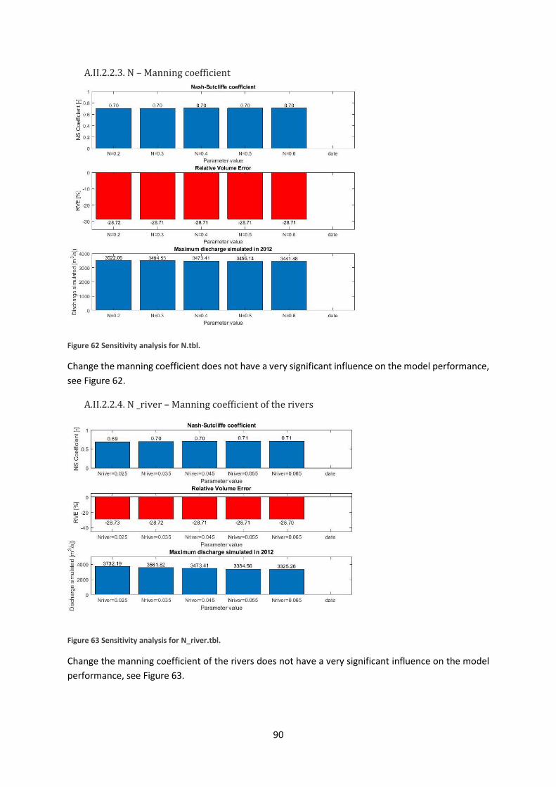
90
A.II.2.2.3. N – Manning coefficient
Figure 62 Sensitivity analysis for N.tbl.
Change the manning coefficient does not have a very significant influence on the model performance,
see Figure 62.
A.II.2.2.4. N _river – Manning coefficient of the rivers
Figure 63 Sensitivity analysis for N_river.tbl.
Change the manning coefficient of the rivers does not have a very significant influence on the model
performance, see Figure 63.
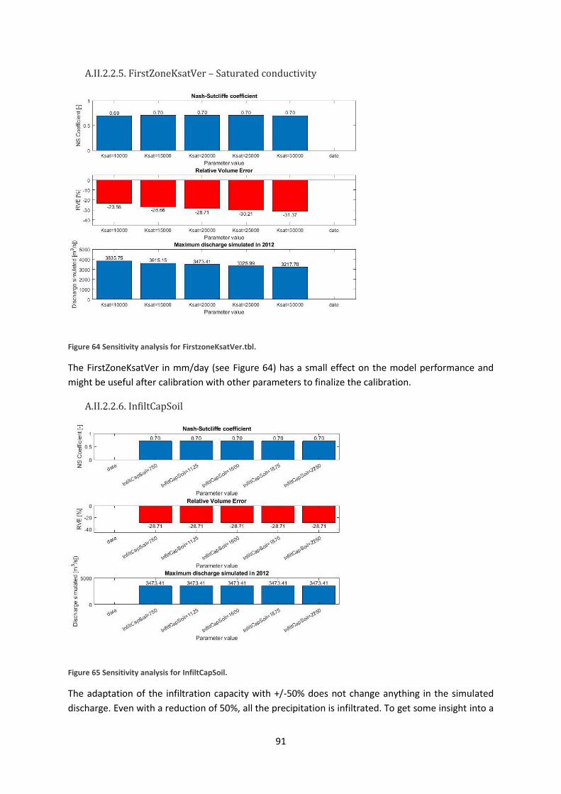
91
A.II.2.2.5. FirstZoneKsatVer – Saturated conductivity
Figure 64 Sensitivity analysis for FirstzoneKsatVer.tbl.
The FirstZoneKsatVer in mm/day (see Figure 64) has a small effect on the model performance and
might be useful after calibration with other parameters to finalize the calibration.
A.II.2.2.6. InfiltCapSoil
Figure 65 Sensitivity analysis for InfiltCapSoil.
The adaptation of the infiltration capacity with +/-50% does not change anything in the simulated
discharge. Even with a reduction of 50%, all the precipitation is infiltrated. To get some insight into a

92
low infiltration capacity this variable is also changed to 10 and 50 mm/day, see Figure 66. This result
in much higher maximum discharges and the model performance decreases significantly.
Figure 66 Sensitivity analysis for InfiltCapSoil.tbl with lower values.
A.II.2.2.7. Conclusion
From the sensitivity analysis, it becomes clear that the first zone capacity, the decay of conductivity
with depth (M) and the saturated conductivity of the store at the surface (FirstZoneKsatVar) are the
most important parameters for the calibration. The current value of the decay of conductivity with
depth results in the best NS coefficient. For the first zone capacity and the FirstZoneKsatVer, there
seem to be good possibilities for improvement.
A.II.2.3. Calibration
The existing model has a NS value of 0.70, a RVE of -29% and a maximum simulated discharge in 2012
of 3473 m3/s, the maximum observed discharge in 2012 at Mount Arayat based on Van ’t Veld (2015)
is 1970 m3/s.
The first parameter that will be calibrated to improve the model performance is the first zone capacity.
After calibrating the first zone capacity, the FirstZoneKSatVar will be calibrated.
A.II.2.3.1. First zone capacity
The results of changing the first zone capacity are presented in Figure 67. There is an optimum of the
NS and RVE with a first zone capacity of 40000 mm. Also, the maximum peak discharge that is
simulated is closer to the measured peak discharge in 2012, which is presented in Figure 68.

93
A first zone capacity of 40 meters is very unrealistic. It shows that the absence of realistic static maps
(land use and soil layer) has a large influence on the reliability of the parameter values and the model
itself.
Figure 67 Wflow calibration of the first zone capacity.
Figure 68 Simulated discharge after calibration first zone capacity.

94
A.II.2.3.2. Saturated conductivity of the store at the surface
The first zone capacity has been set to 40000 mm and the effect of changing the saturated conductivity
of the store at the surface (FirstZoneKsatVer in wflow) has been investigated.
Figure 69 Wflow calibration of the FirstZoneKsatVer.
The NS-coefficient has a maximum with a FirstZoneKsatVer of 30000 mm/day. With increasing the
FirstZoneKsatVer, the maximum discharge tends towards the measured discharge. The discharge with
a FirstZoneKsatVer of 30000 mm/day and a First zone capacity of 40000 mm is presented in Figure 70.
Figure 70 Simulated discharge in 2012 after calibration of saturated conductivity.

95
A.II.2.3.3. Conclusion
Due to the absence of good static maps for the land use and soil layers in the model, the calibration is
very difficult and does not make sense since the link with the physical reality is lost. Therefore, the
calibration is not optimized and the model with a FirstZoneKsatVer of 30000 mm/day and a First zone
capacity of 40000 mm will be used in the validation, despite the fact that both values are considered
very unrealistic.
A.II.2.4. Validation
To validate the model, the discharge of 2013-2014 has been simulated with the new model
parameters. The NS coefficient of the calibrated model is 0.40 and the RVE -39.7%, which is very bad
for a calibrated model. For the uncalibrated model, the NS is 0.31 and the RVE -42.6%. The measured
discharge and the simulated discharges with the calibrated and not calibrated model are presented in
Figure 71 and Figure 72. The accuracy of the model is hardly increased by the calibration. This is
probably caused by the inaccuracy of the precipitation dataset, the wrong catchment area and the
fact that important static maps like land use and soil layer are not determined well in wflow.
A.II.2.4.1. Conclusion
Despite the poor result of the NS coefficient and RVE of the hydrological simulation, the timing and
order of magnitude of the peak discharges seem to correspond well with the measured discharges.
Based on this conclusion, it should be possible to use the model for extreme value analysis and to
draw conclusions about the joint occurrence of storm surge and discharge peaks during typhoons.
Figure 71 Simulated and measured discharges 2013.
0
500
1000
1500
2000
2500
01-07-13 21-07-13 10-08-13 30-08-13 19-09-13 09-10-13 29-10-13 18-11-13
Dis
char
ge (
m3/s
)
Date
Simulated (calibrated) Measured Simulated (not calibrated)
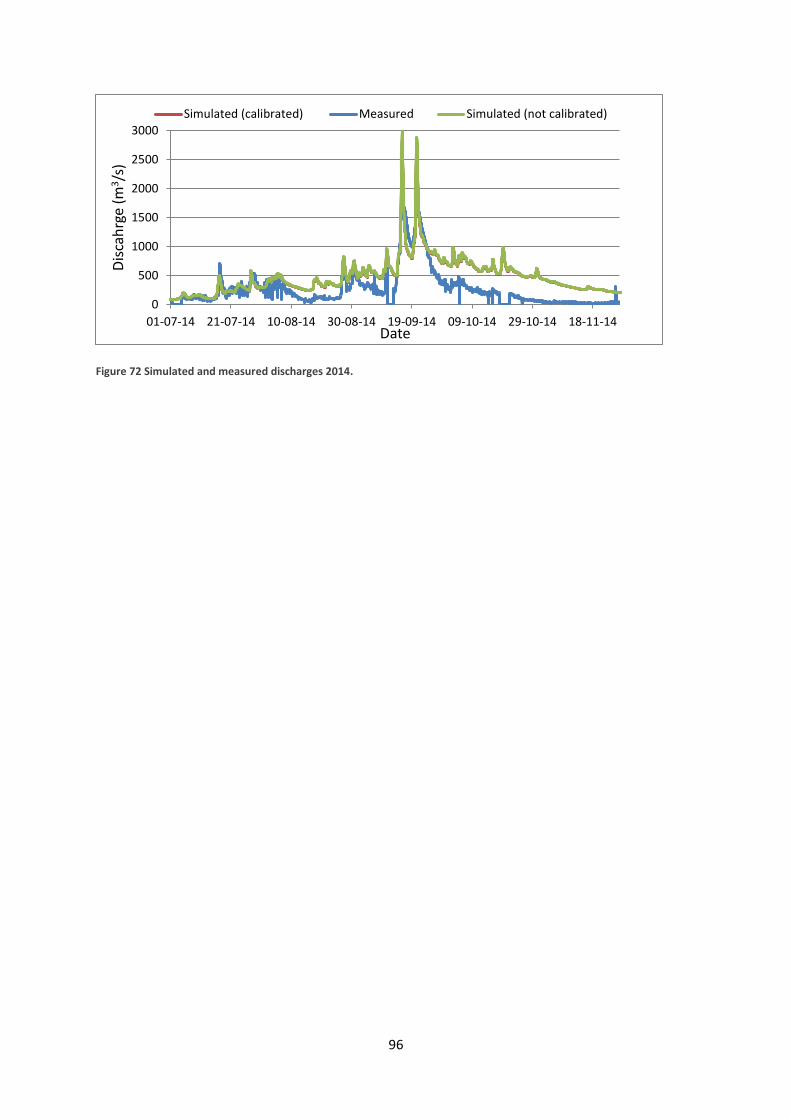
96
Figure 72 Simulated and measured discharges 2014.
0
500
1000
1500
2000
2500
3000
01-07-14 21-07-14 10-08-14 30-08-14 19-09-14 09-10-14 29-10-14 18-11-14
Dis
cah
rge
(m3/s
)
Date
Simulated (calibrated) Measured Simulated (not calibrated)

97
A.III. Inundation simulations with the lowest discharge
boundary
Figure 73 Simulated inundations scenario 1. Discharge, surge and tide peaks together.
Figure 74 Simulated inundations scenario 2. Discharge and tide peaks together, no surge.
Figure 75 Difference in inundations between scenario 1 and 2.

98
Figure 76 Simulated inundations scenario 3. Discharge and surge peaks together during lowest tide.
Figure 77 Difference in inundations between scenario 1 and 3.
Figure 78 Simulated inundations scenario 4. Discharge peaks during lowest tide, no surge.
Figure 79 Difference in inundations between scenario 1 and 4.

99
Figure 80 Simulated inundations scenario 5. Surge and tide peaks together, no discharge.
Figure 81 Difference in inundations between scenario 1 and 5.