coherent minimisation: aggressive optimisation for
TRANSCRIPT

COHERENT MINIMISATION:
AGGRESSIVE OPTIMISATION FOR
SYMBOLIC FINITE STATE
TRANSDUCERS
by
ZAID AL-ZOBAIDI
A thesis submitted toThe University of Birmingham
for the degree ofDOCTOR OF PHILOSOPHY
School of Computer Science
College of Engineering and Physical SciencesThe University of BirminghamJanuary 30, 2014

University of Birmingham Research Archive
e-theses repository This unpublished thesis/dissertation is copyright of the author and/or third parties. The intellectual property rights of the author or third parties in respect of this work are as defined by The Copyright Designs and Patents Act 1988 or as modified by any successor legislation. Any use made of information contained in this thesis/dissertation must be in accordance with that legislation and must be properly acknowledged. Further distribution or reproduction in any format is prohibited without the permission of the copyright holder.


Abstract
Automata are a fundamental model of computation, with many applications in hardware
and software. Automata minimisation is a process of reducing the number of control
states. It is considered as one of the key computational resources that drive the cost of
computation. Most of the conventional minimisation techniques are based on the notion
of bisimulation to determine equivalent states which can be identified.
Although minimisation of automata has been an established topic of research, the
optimisation of automata works in constrained environments is a novel idea which we will
examine in this dissertation, along with a motivating, non-trivial application to efficient
tamper-proof hardware compilation.
This thesis introduces a new notion of equivalence, coherent equivalence, between
states of a transducer. It is weaker than the usual notions of bisimulation, so it leads to
more states being identified as equivalent. The central idea is that if the behaviour of
the environment is restricted, and thus it has a weaker power of distinguishing actions of
an observed system, more states are rendered equivalent. This new equivalence relation
can be utilised to aggressively optimise transducers by reducing the number of states, a
technique which we call coherent minimisation. We note that the coherent minimisation
always outperforms the conventional minimisation algorithms based on the bisimulation
quotienting. The main result of this thesis is that the coherent minimisation is sound and
compositional.
i

In order to support more realistic applications to hardware synthesis, we also introduce
a refined model of transducers, which we call symbolic finite states transducers, that can
model systems which involve very large or infinite data types. As a key motivating
application we give an efficient model for tamper-proofing hardware circuits synthesised
from game-like models.
ii

Acknowledgements
First, I would like to extend my deepest gratitude to my supervisor, Dan Ghica, for
valuable advice, support and guidance during my PhD study.
Next, I would like to thank my thesis group members: Uday Reddy, Peter Breuer,
and Steven Quigley. They have made a significant contribution to this research and their
comments and analysis are highly appreciated.
A great deal of thanks goes to my colleagues: Mohammed Wasouf, Ali Rodan, and
Noureddin Sadawi. They made the daily grind of being a research student so much fun.
Finally, I give my special thanks to my family: my wife Benaz; my mother; my lovely
daughter Naz; and my aunt for their love, support and encouragement.
To all of you, I dedicate this work.

iv

Contents
1 Introduction 11.1 Research Theme . . . . . . . . . . . . . . . . . . . . . . . . . . . . . . . . . . . 11.2 Motivation . . . . . . . . . . . . . . . . . . . . . . . . . . . . . . . . . . . . . . . 31.3 Thesis Outline and Contributions . . . . . . . . . . . . . . . . . . . . . . . . . 51.4 Publications . . . . . . . . . . . . . . . . . . . . . . . . . . . . . . . . . . . . . . 7
2 Background 92.1 Synopsis . . . . . . . . . . . . . . . . . . . . . . . . . . . . . . . . . . . . . . . . 92.2 Finite State Machines . . . . . . . . . . . . . . . . . . . . . . . . . . . . . . . . 9
2.2.1 The Language Accepted by FSM . . . . . . . . . . . . . . . . . . . . . 112.2.2 Other Models of FSM . . . . . . . . . . . . . . . . . . . . . . . . . . . . 112.2.3 Finite States Transducers . . . . . . . . . . . . . . . . . . . . . . . . . 132.2.4 Equivalence of FSMs and States Minimisation . . . . . . . . . . . . . 14
2.3 Hardware Description Languages and VHDL . . . . . . . . . . . . . . . . . . 192.3.1 VHDL Background . . . . . . . . . . . . . . . . . . . . . . . . . . . . . 192.3.2 Behavioural Description of FSM in VHDL . . . . . . . . . . . . . . . 20
2.4 Game Semantics . . . . . . . . . . . . . . . . . . . . . . . . . . . . . . . . . . . 262.4.1 Arenas . . . . . . . . . . . . . . . . . . . . . . . . . . . . . . . . . . . . . 312.4.2 Legal Plays and Strategies . . . . . . . . . . . . . . . . . . . . . . . . . 32
2.5 Hardware Compilation . . . . . . . . . . . . . . . . . . . . . . . . . . . . . . . 322.6 Geometry of Synthesis Hardware Compiler . . . . . . . . . . . . . . . . . . . 34
2.6.1 The Language Verity . . . . . . . . . . . . . . . . . . . . . . . . . . . . 342.6.2 Theoretical and Methodological Background of Verity-GoS . . . . . . 362.6.3 Interpreting the Verity Constants . . . . . . . . . . . . . . . . . . . . . 37
2.7 Tampering and Tamper-Proof . . . . . . . . . . . . . . . . . . . . . . . . . . . 452.8 Summary . . . . . . . . . . . . . . . . . . . . . . . . . . . . . . . . . . . . . . . 46
3 Concurrent Finite States Transducers (CFSTs) 473.1 Synopsis . . . . . . . . . . . . . . . . . . . . . . . . . . . . . . . . . . . . . . . . 473.2 Legal Interactions (Protocol) . . . . . . . . . . . . . . . . . . . . . . . . . . . . 503.3 Two Ways of Composing CFSTs . . . . . . . . . . . . . . . . . . . . . . . . . . 52
3.3.1 CFSTs Intersection . . . . . . . . . . . . . . . . . . . . . . . . . . . . . 523.3.2 CFSTs Composition . . . . . . . . . . . . . . . . . . . . . . . . . . . . . 54
v

3.4 Behavioural Description of CFSTs in VHDL . . . . . . . . . . . . . . . . . . 583.5 Chapter Summary . . . . . . . . . . . . . . . . . . . . . . . . . . . . . . . . . . 62
4 Coherent Minimisation 634.1 Synopsis . . . . . . . . . . . . . . . . . . . . . . . . . . . . . . . . . . . . . . . . 634.2 CFST Language . . . . . . . . . . . . . . . . . . . . . . . . . . . . . . . . . . . 634.3 Conventional-Equivalence of CFSTs . . . . . . . . . . . . . . . . . . . . . . . . 654.4 Coherent Equivalence of CFSTs . . . . . . . . . . . . . . . . . . . . . . . . . . 734.5 State Reductions for CFSTs . . . . . . . . . . . . . . . . . . . . . . . . . . . . 854.6 Determinism . . . . . . . . . . . . . . . . . . . . . . . . . . . . . . . . . . . . . 894.7 Discussion . . . . . . . . . . . . . . . . . . . . . . . . . . . . . . . . . . . . . . . 93
5 Symbolic Finite State Transducers (SFSTs) 955.1 Synopsis . . . . . . . . . . . . . . . . . . . . . . . . . . . . . . . . . . . . . . . . 955.2 Symbolic Finite State Transducers (SFSTs) . . . . . . . . . . . . . . . . . . . 965.3 Coherent Minimisation in SFSTs . . . . . . . . . . . . . . . . . . . . . . . . . 995.4 Chapter Summary . . . . . . . . . . . . . . . . . . . . . . . . . . . . . . . . . . 114
6 Case Study: Efficient Tamper-Proof Hardware Compilation 1176.1 Synopsis . . . . . . . . . . . . . . . . . . . . . . . . . . . . . . . . . . . . . . . . 1176.2 Verity Constants as Circuits . . . . . . . . . . . . . . . . . . . . . . . . . . . . 1186.3 Protocols and Low-level Attacks . . . . . . . . . . . . . . . . . . . . . . . . . . 1246.4 Enforcing Programming Language Abstractions . . . . . . . . . . . . . . . . 1276.5 Discussion . . . . . . . . . . . . . . . . . . . . . . . . . . . . . . . . . . . . . . . 131
7 Coherent Minimisation for GoS 1357.1 Synopsis . . . . . . . . . . . . . . . . . . . . . . . . . . . . . . . . . . . . . . . . 1357.2 Coherent Minimisation for Verity Constants . . . . . . . . . . . . . . . . . . . 135
7.2.1 Minimal CFSTs are not Unique . . . . . . . . . . . . . . . . . . . . . . 1467.3 Symbolic Coherent Minimisation of Verity Constants . . . . . . . . . . . . . 1477.4 Discussion . . . . . . . . . . . . . . . . . . . . . . . . . . . . . . . . . . . . . . . 150
8 Conclusion and Future Work 1518.1 Conclusion . . . . . . . . . . . . . . . . . . . . . . . . . . . . . . . . . . . . . . . 1518.2 Future Work . . . . . . . . . . . . . . . . . . . . . . . . . . . . . . . . . . . . . 154
Bibliography 159
A VHDL Constructs 173
B Behavioural Description of CFST 175
C Coherent Minimisation for Verity Constants 179
D Formal Proofs of Coherent Minimisation in Agda 185
vi

List of Figures
2.1 Mealy machine for a sequence detector . . . . . . . . . . . . . . . . . . . . . . 132.2 A DFSM defined over {a, b}∗: every literal a is followed by the literal b. . . 162.3 M ′: Minimised DFSM of Fig.2.2. . . . . . . . . . . . . . . . . . . . . . . . . . 182.4 Structure of a Mealy machine with One Logic . . . . . . . . . . . . . . . . . 212.5 Mealy machine for an odd number of 0 and an odd number of 1. . . . . . . 222.6 The play of ’1’ in game semantics represented as a FST. . . . . . . . . . . . 272.7 Verity ’∆’ Constant as an FST. . . . . . . . . . . . . . . . . . . . . . . . . . . 43
3.1 Asynchronous game-semantics protocol represented as an FST. . . . . . . . 513.2 Synchronous protocol (P ) of com1 ⊗ com2⊸ com3 represented as an CFST. 523.3 CFST T : Synchronous representation of the sequential composition constant. 533.4 Sketch of CFSTs interaction. . . . . . . . . . . . . . . . . . . . . . . . . . . . . 553.5 CFSTs interaction . . . . . . . . . . . . . . . . . . . . . . . . . . . . . . . . . . 573.6 CFST T ⊙ T ′ ∶ composition of CFSTs presented in Fig. 3.5a and Fig. 3.5b. 58
4.1 Transducer T . . . . . . . . . . . . . . . . . . . . . . . . . . . . . . . . . . . . . . 754.2 Protocol P . . . . . . . . . . . . . . . . . . . . . . . . . . . . . . . . . . . . . . . 764.3 CFSTs Minimisation. . . . . . . . . . . . . . . . . . . . . . . . . . . . . . . . . 884.4 Generated NCFST (output-nondeterminism) from quotienting two states. . 904.5 Compatible-states relation is intransitive. . . . . . . . . . . . . . . . . . . . . 904.6 Generated NCFST (target-nondeterminism) from quotienting two states. . 924.7 Coherently minimised DCFST of Fig. 4.3a. . . . . . . . . . . . . . . . . . . . 92
5.1 DCFST of m + n. . . . . . . . . . . . . . . . . . . . . . . . . . . . . . . . . . . . 965.2 T : Adding numbers in SFST. . . . . . . . . . . . . . . . . . . . . . . . . . . . 1085.3 Symbolic Protocol P for adding numbers. . . . . . . . . . . . . . . . . . . . . 1105.4 T ∩P : Symbolically intersecting Fig. 5.2 and Fig. 5.3. . . . . . . . . . . . . . 1105.5 T ′ = T /(s1, s2): Coherently minimised SFST of Fig. 5.2. . . . . . . . . . . . 1125.6 T ′∩P : Symbolically intersecting Fig. 5.5 and Fig. 5.3. . . . . . . . . . . . . . 1125.7 T ′′: Coherently Minimal SFST of Fig. 5.2. . . . . . . . . . . . . . . . . . . . . 1135.8 T ′′∩P : Symbolically intersecting Fig. 5.6 and Fig. 5.3. . . . . . . . . . . . . 114
6.1 The diagonal circuit ∆ . . . . . . . . . . . . . . . . . . . . . . . . . . . . . . . 1216.2 The Iterator circuit . . . . . . . . . . . . . . . . . . . . . . . . . . . . . . . . . 122
vii

6.3 Example of synthesised program using the FFI . . . . . . . . . . . . . . . . . 1256.4 Environment which breaks language abstraction . . . . . . . . . . . . . . . . 1266.5 Architecture of a tamper-proof circuit . . . . . . . . . . . . . . . . . . . . . . 1286.6 A game-semantic protocol, automaton representation . . . . . . . . . . . . . 1296.7 Synchronous representation of a protocol . . . . . . . . . . . . . . . . . . . . 1306.8 Tamper-proof compiled circuit with monitor . . . . . . . . . . . . . . . . . . 130
7.1 Protocol of com1 ⊗ com2 ⊸ com3 represented as a CFST. . . . . . . . . . . . 1377.2 Verity conditional ’if ’ constant represented as a CFST. . . . . . . . . . . . . 1407.3 Protocol of var1⊸ exp2 represented as a CFST. . . . . . . . . . . . . . . . . 1407.4 Verity dereferencing constant represented as a CFST. . . . . . . . . . . . . . 1417.5 Optimised Verity diagonal constant by coherent minimisation and consid-
ering Def. 4.6.2. . . . . . . . . . . . . . . . . . . . . . . . . . . . . . . . . . . . . 1427.6 Optimised Verity parallel composition constant by coherent minimisation. . 1447.7 The iterator constant and its protocol. . . . . . . . . . . . . . . . . . . . . . . 1457.8 Optimised Verity iterator ’while’ constant by coherent minimisation and
considering Def. 4.4.4. . . . . . . . . . . . . . . . . . . . . . . . . . . . . . . . . 1467.9 Another possible minimal Verity iterator ’while’ constant. . . . . . . . . . . 1477.10 Input and output ports for the binary addition constant in Verity . . . . . 1487.11 Symbolic Protocol of exp1 ⊗ exp2 ⊸ exp3 represented as a SFST. . . . . . . 1487.12 Verity binary addition constant represented as a SFST. . . . . . . . . . . . . 1497.13 Optimised Verity binary addition constant by symbolic coherent minimisation.149
C.1 Protocol of exp1 ⊗ exp2 ⊸ exp3 represented as a CFST. . . . . . . . . . . . . 180C.2 Verity binary addition constant represented as a CFST. . . . . . . . . . . . . 181C.3 Optimised Verity binary addition operator constant by coherent minimisation.181C.4 Protocol of var ⊗ exp1 ⊸ com2 represented as a CFST. . . . . . . . . . . . . 182C.5 Verity assignment constant represented as a CFST. . . . . . . . . . . . . . . 182C.6 Optimised Verity assignment constant by coherent minimisation. . . . . . . 183
viii

List of Tables
4.1 Compatibility and Coherent Equivalence Relations of Fig.4.3a. . . . . . . . 91
7.1 Results of Minimisation for Verity Constants. . . . . . . . . . . . . . . . . . . 136
C.1 Coherent Minimisation for Verity Constants in Detail. . . . . . . . . . . . . . 179
ix

x
Listings
2.1 Hopcroft’s DFSM Minimisation Algorithm . . . . . . . . . . . . . . . . . . . 162.2 States-assignment in VHDL. . . . . . . . . . . . . . . . . . . . . . . . . . . . . 222.3 Transitions-Encoding of Fig. 2.5 in VHDL. . . . . . . . . . . . . . . . . . . . 232.4 Checking the Rising Edge of the Clock in VHDL. . . . . . . . . . . . . . . . 242.5 Reset-Checking in VHDL. . . . . . . . . . . . . . . . . . . . . . . . . . . . . . 252.6 VHDL Code of Fig. 2.5. . . . . . . . . . . . . . . . . . . . . . . . . . . . . . . . 253.1 CFST-Encoding Algorithm. . . . . . . . . . . . . . . . . . . . . . . . . . . . . 604.1 CFST Minimisation Algorithm. . . . . . . . . . . . . . . . . . . . . . . . . . . 87A.1 Syntax of “If” Statement in VHDL. . . . . . . . . . . . . . . . . . . . . . . . . 173A.2 Syntax of “Case” Statement in VHDL. . . . . . . . . . . . . . . . . . . . . . . 173B.1 VHDL Code of Fig. 3.5a. . . . . . . . . . . . . . . . . . . . . . . . . . . . . . . 175
xi

xii

CHAPTER 1
Introduction
1.1 Research Theme
Automata (or state machines) are labelled transition systems consisting of a set of control
states and a set of transitions. Control moves from one state (source state) to another
(target state) in response to external events. The transitions define the behaviour of the
control states by specifying a relation between source states, external events (input and
output), and target states. If the set of control states of the automata is finite then they
are called finite automata (or finite states machines (FSMs)).
Bisimulation, regarded as one of the key contributions of concurrency theory to Com-
puter Science, is a way of matching processes that requires equivalence between all corre-
sponding control states. In theory, bisimulation is a binary relation associating two control
states that behave in the same way. Intuitively, two states are bisimilar if each state can
not be distinguished from the other by an observer. The bisimulation equality (also called
bisimilarity) is the most popular form of behavioural equality for processes [46, 120]. The
compositionality property of bisimilarity has been utilised to optimise the state-space of
processes represented by automata [120].
1

FSM minimisation is about reducing the number of control states such that the op-
timised FSM is behaviourally equivalent to the original one. In general, the process of
minimisation is twofold: identifying the bisimilar states and then quotienting them.
Of the many applications of FSMs, hardware synthesis is of clear practical importance.
FSMs are convenient models of representation for sequential circuits at a logical level of
abstraction. Minimising the number of states will optimise the size of the machine for
subsequent steps in the synthesis. As a result, fewer hardware resources are required in
the synthesised circuit [77, 130].
Game semantics is an approach to denotational semantics that provides correct and
sound fully abstract models for several programming languages, some of which can be
given automata-theoretic representations [57, 6]. In game semantics, types are interpreted
as arenas (or games) between the term (system) being modelled and the environment in
which the term being used. Arenas are sets of game moves which can be either question
or answer and belong to either the term or the environment. Game semantics uses
mathematical objects called strategies to represent terms [4, 8]. Strategies obey the rules
of games and they describe the behaviour of the system—how the system should interact
with its environment [63, 50]. Game play (or shortly play) is a sequence of moves. Each
strategy is defined as a set of plays and can sometimes be represented by a set of its legal
traces over the alphabet of moves, and hence by an automaton.
Hardware compilation is a process of translating programs written in high-level lan-
guages into hardware circuits. This technology is gaining popularity because it provides
“software-like” environments and hence it can be used by many users [126, 26]. There are
many hardware compilation approaches, most of them depend on the idea of extending
one of the conventional programming languages with explicit constructs to provide means
of concurrency and parallelism. Another promising approach, suggested and studied by
Ghica, is called Geometry of Synthesis [49, 60, 61, 62]. The most appealing feature of
2

this technique is that its models, which can be represented as automata, are concrete
representations of the denotational model of the language, therefore leading to correct-
by-construction compilation. Geometry of Synthesis (GoS) exploits the existence of a
natural correspondence between the fundamental notions of game semantics and those of
digital circuits, and hence the automata-based models of GoS can be translated directly
into hardware circuits.
1.2 Motivation
The games-based approach to hardware compilation exploits the natural connections
between hardware and game semantics concepts. In addition to giving a correct-by-
construction, semantics-directed hardware compilation method, the existence of well-
defined access protocol to interfaces supports features such as libraries, separate com-
pilation and even foreign function interfaces (FFI). These are all essential features of a
mature compiler. The FFI especially, is instrumental in accessing the physical resources of
an arbitrary system or pre-existing libraries of IP cores using the function call mechanism.
However, interfacing with circuits produced outside the compiler exposes the synthesised
code to low-level attacks (tamper attempts), because such circuits cannot be guaranteed
to satisfy the input-output protocol which synthesised circuits must satisfy and assume in
order to operate properly. Circuits generated naively from the game semantic models are
tamper-resistant by construction because they cannot handle illegal environment actions.
However, having tamper-resistance built-in compositionally is extremely inefficient.
In this thesis we examine the possibility of more optimisation opportunities in au-
tomata representing game-semantic models of programs. These type of automata are
meant to operate in environments whose input-output behaviour is constrained by the
rules of a game (protocol). Since not all actions are available to the environment, then
this may lead to a notion of equivalence between states which is weaker than the con-
3

ventional notion of bisimulation, and hence more states are being identified as equivalent
and consequently leading to more aggressive optimisations.
In conventional automata optimisation, two states are considered equivalent if they
are not distinguishable by any environment; this concept is formalised by bisimulation.
Bisimilar states can be identified, leading to optimised automata with fewer states. Min-
imising automata in restricted environments has not been considered in the literature,
although Pierce and Sangiorgi have introduced related ideas for mobile processes under
the name of “behavioural equivalence” [108, 109] which is based on the barbed bisimula-
tion [97]. However, from the way it is formulated, it is difficult to observe the properties
of control states from their corresponding processes.
Representing game semantics models by finite automata has been presented in the
literature [54, 57]. Moving beyond finite automata has also been considered either di-
rectly [75] or via abstract interpretation [40, 41]. Both these approaches have been used
in model checking of software, but they are not suitable for hardware synthesis. In order to
compile systems which involve numerical values without the problem of having very large
(or infinite) numbers of states, we will present a refined model of automata which uses
symbolic representations of states as registers, in addition to the conventional concrete
ones used for control. Several transitions from one source state to different destination
states can be interpreted by one transition governed by a symbolic condition. This sug-
gested model of automata is actually inspired by the work of Bakewell and Ghica [16],
but the technical details are significantly different. These models were introduced for the
purposes of model checking and hence there is no enough abstraction can be utilised by
the relations of states simulation and equivalence.
To bring all these ideas together we propose, as a case study, an efficient way to
synthesis tamper-proof hardware circuits from programs written in conventional languages
using the GoS methodology and compiled to circuits via finite-state or symbolic automata.
4

1.3 Thesis Outline and Contributions
The thesis is organised as follows:
1 – Introduction.
2 – Background. Formally introduces the fundamental concepts we use in the
rest of the work. It reviews FSMs and their models. This review pays particular at-
tention to some concepts such as equivalence, composition and minimisation, which
are relevant to our research. Chapter 2 also gives a brief introduction to hardware
description languages (HDLs) followed by game semantics and hardware compila-
tion, in particular Geometry of Synthesis hardware compiler (GoS). This chapter
concludes with a brief overview on the problem of tampering in hardware circuits.
3 – Concurrent Finite States Transducers. Introduces a suitable model of
finite state transducers (FSTs), which we call concurrent finite state transducers
(CFSTs), with examples to show how CFSTs can be intersected and composed.
Also in this chapter we discuss how programming language types can be seen as
protocols. Finally, we present an algorithm for generating VHDL code from CFSTs.
4 – Coherent Minimisation. This is the key conceptual and theoretical contribu-
tion of the thesis, where we define a novel equivalence relation, coherent equivalence,
which is weaker than the conventional equivalence relation and motivated by the
existence of a restricted interaction between the system and its environment. The
main result of the thesis is to show that coherent equivalence is sound. We give the
(standard) minimisation algorithm based on this notion of equivalence. Since we are
dealing with a compiler, the concept of the compositionality is very important as
the coherent minimisation can be applied to any sub-component of a larger system
without affecting its overall properties, including the coherence equivalence itself.
5

The second main result of this thesis is that the coherent equivalence not only
sound but also compositional. Finally, we discuss the subtle connection between
determinism and coherence minimisation in CFSTs, as it is particularly relevant to
hardware synthesis.
5 – Symbolic Finite States Transducers. Discusses the limitations of CFSTs
and proposes an improved model of infinite state transducers with finite control,
which we call symbolic finite state transducers (SFSTs). We also adapt the notion
of protocol to symbolic representation, and define intersection between the symbolic
protocol and SFSTs. Subsequently, we present a modified definition of coherent
equivalence relation (symbolic coherent equivalence) which identifies the equivalent
states in SFSTs. Finally, we discuss by example how SFSTs can be coherently min-
imised by identifying coherent equivalent states. As in the case of CFSTs, we prove
that the relation of symbolic coherence is sound and we note that the composition-
ality property of symbolic coherent minimisation is an immediate consequence of
the compositionality of coherent minimisation of CFSTs.
6 – Case Study: Efficient Tamper-Proof Hardware Compilation. In this
chapter we propose a model that can detect and resist low level attacks on hardware
compilation by monitoring the interactions between the program and its environ-
ment. We demonstrate that tamper-proof hardware compilation can be achieved
efficiently by restricting the synthesised circuit to interact with its environment
through an interface enforcing a protocol, which detects any illegal interaction.
This allows us to assume that indeed the behaviour of the environment is restricted
and use coherent (symbolic) equivalence to reduce the number of states in the rep-
resentation of the circuit.
6

7 – Coherent Minimisation for GoS. We examine the effectiveness of coherent
minimisation by comparing the coherent minimisation results to those of bisimula-
tion quotienting.
8 – Conclusions and Future Work. We conclude by summarising our results
and proposing possible future directions which can be done to extend this research.
1.4 Publications
This thesis is partly based upon the following publication:
Dan R. Ghica and Zaid Al-Zobaidi. Coherent minimisation: Towards efficient
tamper-proof compilation. EPTCS,104: 83–98, 2012.
This paper has been presented by Zaid Al-Zobaidi in the Fifth Interaction and Con-
currency Experience (ICE) Workshop.
Olle Fredriksson, Dan R. Ghica and Zaid Al-Zobaidi. Certified minimisation of
automata under protocol. (in preparation)
7

8

CHAPTER 2
Background
2.1 Synopsis
In this chapter, we review finite state machines and introduce the common models of FSMs
and other important concepts which are relevant to this thesis, in particular equivalence
and minimisation. This chapter also presents the hardware description languages (HDLs)
and explores how the functional behaviour of FSMs can be encoded using these languages.
This is followed by a background on game semantics and hardware compilation. Finally,
we conclude by reviewing the problem of circuits tampering.
2.2 Finite State Machines
Finite state machines (FSMs) are a common and very useful model of computation. For-
mally a FSM can be defined as a tuple ⟨S,Σ, s0, δ,F ⟩, consisting of:
• A finite set of states, S.
• A finite set of input symbols, Σ.
• A designated initial state (start state), s0 such that s0 ∈ S.
9

• A transition function, δ, that takes a state (source state) and an input symbol and
returns a state (target state), δ ∶ S ×Σ → S.
• A finite set of final states (accept states), F , such that F ⊆ S.
FSM can be in only one state (internal configuration) at a time. Note that, in this thesis
we indicate a component of FSM M by writing M as a subscript.
The previous definition is for a specific type of FSM which is called Deterministic
(DFSM). A FSM M is said to be deterministic if for every state s ∈ S and for every
input symbol a ∈ Σ, there is only one target state can be accessed by reading a from s.
By contrast, a FSM M is called Non Deterministic (NFSM) if the previous condition is
not satisfied. The only difference between DFSM and NFSM is how the transitions are
defined. In NFSM the transition relation (δ) is defined as a finite subset of S ×Σ×S. The
transition relation can be extended from taking one input symbol to a string (sequence
of input symbols). We will call this relation the extended transition relation and it will
be denoted by δ. It is defined inductively on strings as δ ⊆ S × Σ∗ × S. Similarly, the
transition function in DFSM can be extended to strings and defined as δ ∶ S ×Σ∗ → S.
As in any directed graph, a FSM is said to be connected if there is a path from the
initial state (start state) to all other states, ∀q ∈ S,∃w ∈ Σ∗ s.t (s,w, q) ∈ δ. Unreachable
states can be detected and removed to make the FSM initially connected.
Another important concept in DFSM is completeness. A DFSM is called complete if
from every state and for every input symbol the transition function is defined, in other
words the transition function is a total function. An incomplete DFSM can be transformed
to a complete version by introducing a special state (called dummy state) and by assigning
the target state of all missing transitions to the dummy state [82, 123].
10

2.2.1 The Language Accepted by FSM
The language that is accepted by any FSM can be defined as a set of all strings that
result in a sequence of transitions that takes the FSM from the start state to one of the
final states. Formally, the language of a DFSM M , written JMK, can be defined as follows:
JMK = {w ∣ δM(s0
M ,w) ∈ FM}
Similarly, the language of NFSM M can be defined as follows:
JMK = {w ∣ (s0
M ,w, q) ∈ δM and q ∈ FM}
2.2.2 Other Models of FSM
From our presented definition of FSM we can deduce that there are only two possibilities of
output: accept or reject in correspondence to final states and non-final states, respectively.
There are situations that require more than two kinds of output, and hence many models
of FSMs have been suggested and presented in the literature [82, 123] to deal with the
output alphabets of other domains. These models can be broadly classified into two
types: FSM with output associated with states (Moore Machine) and FSM with output
associated with transitions (Mealy Machine).1 Although the Mealy machine is a more
popular formalism, it is well known that the Moore formalism is as expressive and there
is a classic algorithm for converting between the two machines.
A Mealy machine M can be formally defined by the following tuple:
M = ⟨SM ,ΣM ,ΓM , s0
M , δM ⟩
1 The name of Moore and Mealy machines are in honour of Edward Moore and George Mealy, whodescribe the behaviour of these machines for the first time in the 1950s.
11

The components of the machine are:
• A finite set of states, SM .
• A finite set of input symbols, ΣM .
• A finite set of output symbols, ΓM .
• A designated initial state, s0
M such that s0
M ∈ SM .
• A transition function, δM ∶ SM ×ΣM Ð→ SM × ΓM
To understand how Mealy machines work we need to realise how the transitions can
be interpreted. Let us consider we have δ(q, i) = (q′, o) as one of the transitions of a Mealy
machine M then this means: if the machine M at state q reads the input i then it will
produce the output o and move to the next state q′. This can be represented graphically
as follows:
q q′i/o
FSMs, including Mealy machines, can be represented by a transition diagram, which
is a directed graph whose vertices correspond to the states of the machine while its edges
stand for the transitions of the machine. These edges are labelled by the associated input
and output.
Example 2.2.1 Let us consider the problem of a sequence detector and we want to design
a Mealy machine that outputs ‘A’ when it detects the input sequence ‘101’ , outputs ‘B’
when it detects ‘100’, and outputs ‘C’ in all other cases.
In this example we have Σ = {0,1} while the set of output symbols Γ = {A,B,C}. The
machine can be represented as a state diagram as shown in Fig. 2.1.
12

q0 q1
q2
0/C 1/C
1/C
0/C
1/A
0/B
Figure 2.1: Mealy machine for a sequence detector
Recalling the presented formal definition of the Mealy machine, it might be useful to
define the output function explicitly in the tuple instead of being part of the transition
function. The output function, λ can be defined as S ×Σ → Γ. By removing the output
from the transition function, we will have δ as S ×Σ → S. However, the new formal defi-
nition of Mealy machines is functionally equivalent to the former one and also presented
in several literature [82, 116]. Moore machine is another model which can be used to
represent FSM with outputs that can be formally defined in a similar way to the second
formal definition of Mealy machines apart from the output function. Since its outputs
are associated with the states only, then the output function λ will be defined as S → Γ,
which means every state has a specific output.
2.2.3 Finite States Transducers
In Sec. 2.2.2 we presented the Mealy machine, whose outputs are determined by inputs
and its current state. A Finite States Transducer (FST) is a non-deterministic Mealy
machine that may exclude input and/or the output from the transitions [85, 76, 20].
Formally, a FST is defined by a 5-tuple as follows [85, 76]:
⟨S,Σ,Γ, s0, δ⟩
13

All components of FSTs, apart from the transition relation δ, are similar to those
defined previously for Mealy machines, while the transition relation δ can be defined as a
finite subset of S × (Σ ∪ {ǫ}) × (Γ ∪ {ǫ}) × S.
In the literature it has been shown that FSTs are closed under many operations, in
particular composition [85]. Composition is one of the key operations that can be applied
on transducers. Given two transducers T and T ′ defined over the same input and output
alphabets, the composition of T and T ′ is a transducer T ⊙ T ′ defined by the following
tuple:
⟨ST × ST ′ ,Σ,Γ, (s0
T , s0
T ′), δT⊙T ′⟩
where δT⊙T ′ is defined as follows:
((s, s′), i, o′, (q, q′)) ∈ δT⊙T ′ if and only if (s, i, o, q) ∈ δT and (s′, o, o′, q′) ∈ δT ′
2.2.4 Equivalence of FSMs and States Minimisation
There are different points of view which can be considered in the criteria of FSMs equiv-
alence. Those variations are highly dependent on the type of FSMs. If two FSMs are
FSMs with final states, then they are equivalent if and only if they accept the same set of
strings (same language). On the other hand, if FSMs are transducers, Mealy, or Moore
machines, then two FSMs are equivalent if and only if they produce two identical outputs
as a response to the same input sequence [20]. Intuitively, equivalent states can be defined
in terms of equivalence of FSMs. We can say two distinct states, s′ and s′′, in any FSM
M are equivalent if FSMs Ms′ and Ms′′ are equivalent, where Ms′ means a modified FSM
M with start state s′. More precisely, for any arbitrary FSM M = ⟨SM ,ΣM , sM , δM , FM ⟩
and any two states s′, s′′ ∈ SM we have the following:
J⟨SM ,ΣM , s′, δM , FM ⟩K = J⟨SM ,ΣM , s′′, δM , FM⟩K if and only if s′ ≡ s′′
14

Having two equivalent states it means that one of the states is redundant and can be
eliminated. As a result, the number of the states is reduced. Writing an efficient algorithm
for minimizing DFSM has a long history. The time complexity of most minimising algo-
rithms is O(n2) , where n is the number of states. Hopcroft’s algorithm has become one of
the popular minimising algorithms because of its time complexity of O(n log n) [81, 110].
Hopcroft’s algorithm depends on the idea of finding equivalence classes. The states are
partitioned into disjoint blocks such that every block contains only states that behave
similarly in correspondence to the inputs. Initially, the minimisation process starts with
only two blocks: one contains all the final states (F ) and the second consists of all the
remaining states (S − F ). The refining process of the blocks lasts for several iterations
until no new block can be introduced and hence the minimisation operation terminates.
The number of states in the minimised DFSM is the final number of the blocks. In the
resulting minimised DFSM all states that are in one block will be merged into one state.
Several DFSMs can be designed to accept the same language. We say that M is a minimal
DFSM if and only if there is no other DFSM that accepts the same language of M and
has fewer states than M . In fact, for every regular language there is only one minimal
DFSM [82, 116]. Hopcroft’s algorithm has been introduced for the first time in [81] and
has been studied and revisited several times in many publications [21, 90, 110]. Hopcroft’s
algorithm [24] is outlined in Lst. 2.1. Note that, the splitting of the set H by the pair
(Q,a) in line 7 occurs if and only if:
δ(H,a) ∩Q ≠ ∅ and δ(H,a) ∩ (S/Q) ≠ ∅ (2.1)
while by δ(H,a) we denote the set {p∣p = δ(q, a), q ∈H}. Finally, the two subsets H ′ and
H ′′ in line 8 are generated from H as follows:
H ′ = {q ∈H ∣δ(q, a) ∈ Q} and H ′′ = H/H ′ (2.2)
15

Listing 2.1: Hopcroft’s DFSM Minimisation Algorithm
1: let ρ = {{F},{S − F}}2: let X= Minimum (F,S −F )3: for all a ∈ Σ do
4: add(X,a) to the list l
5: while l ≠ ∅ do
6: extract (Q,a) from the list l
7: for each block H ∈ ρ that is split by (Q,a) do
8: generate H ′,H ′′ as new blocks resulting from
splitting of H w.r.t (Q,a)9: replace H in ρ with H ′,H ′′
10: let Y= Minimum (H ′,H ′′)11: for all b ∈ Σ do
12: if (H,b) ∈ l then
13: replace (H,b) with (H ′, b), (H ′′, b)14: else
add(Y, b) to the list l
In the following example we will show how Hopcroft’s algorithm can minimise a DFSM.
Example 2.2.2 Consider the DFSM M defined by the following tuple:
⟨{s0, s1, s2, s3, s4},{a, b}, s0, δ,{s0, s2}⟩
where δ is depicted in Fig. 2.2.
s0 s1 s2
s3s4
b
a
a
b
b
ab
a
b
a
Figure 2.2: A DFSM defined over {a, b}∗: every literal a is followed by the literal b.
16

Obviously, the DFSM shown in Fig. 2.2 has Σ = {a, b} and accepts all strings over
Σ∗ that have every literal ’a’ followed by the literal ’b’. The application of Hopcroft’s
algorithm to minimise this DFSM can be summarised in the following steps:
1. Initially ρ = {{s0, s2},{s1, s3, s4}}.
2. X = {so, s2}
3. Add the pairs ({s0, s2}, a), ({s0, s2}, b) to the list l. We will assume that the list l
is a stack.
4. Since l ≠ ∅, continue with the following steps in the algorithm.
5. Extract ({s0, s2}, b) from the stack l, so we have Q = {s0, s2} and S/Q = {s1, s3, s4}
6. (a) Examine the first block {s0, s2}, denoted by H1, against the extracted pair
(Q,b). It is clear that δ(H1, b) is {s2} and hence {s2} ∩ Q ≠ ∅. However,
{s2} ∩ (S/Q) = ∅, which means no splitting operation will occur in the block
H1, as specified in (2.1).
(b) Examine the other block {s1, s3, s4}, denoted by H2, against the extracted pair
(Q,b). Obviously, δ(H2, b) is {s2, s3}. Since {s2, s3} ∩ Q ≠ ∅ and {s2, s3} ∩
(S/Q) ≠ ∅, then the condition of partitioning in (2.1) is satisfied and hence the
block H2 will be replaced by the two sub bocks {s3, s4} and {s1}, as specified
in 2.2. Consequently, ρ = {{s0, s2},{s3, s4},{s1}}. Because ({s1, s3, s4}, a) ∉ l
and since {s1} is the smallest block (only one state) we need to add the pair
({s1}, a) to l. Likewise, the pair ({s1}, b) will be added to l. After the last
modifications, the list l contains the following pairs (in order):
{({s1}, b), ({s1}, a), ({s0, s2}, a)}.
17

7. Step 6 will be repeated with all pairs in list l until the list becomes empty. Thus
the algorithm will terminate with:
ρ = {{s0, s2},{s3, s4},{s1}}.
As outlined above in Step 7, minimising the DFSM M ends up with only three
states, ({{s0, s2},{s3, s4},{s1}}), instead of the original five states. In other words,
s0 ≡ s2 and s3 ≡ s4, which can be interpreted as s2 and s4 are redundant states. We
will denote the minimised DFSM by M ′, which can be defined by the following tuple:
⟨{{s0, s2},{s3, s4},{s1}},{a, b},{s0, s2}, δ′,{{s0, s2}}⟩
where δ′ is given by the state diagram shown in Fig. 2.3. By reviewing Fig. 2.3 and
comparing it to Fig. 2.2 it is obvious that JMK = JM ′K.
{s0, s2} {s1}
{s3, s4}
a
b
b
a
a, b
Figure 2.3: M ′: Minimised DFSM of Fig.2.2.
It is important to mention that the equivalence relation on control states is reflexive,
symmetric and transitive but only for a complete DFSM. In an incomplete DFSM the
property of transitivity will be void, and hence the relation is no longer called equivalence,
but is rather called compatibility. The definition of this relation will not be revisited here
18

but it is discussed in the literature [116, 119].
2.3 Hardware Description Languages and VHDL
Hardware Description Languages (HDLs) are languages that are mainly used to describe
hardware systems for different purposes. The main difference between HDLs and conven-
tional programming languages, such as C, is that HDLs are used to describe and implement
hardware circuits while the conventional languages are used mainly to write code that will
be executed on a computer. Furthermore, HDLs provide concurrent execution not just
sequential [101].
HDLs can be used to describe any hardware system at different levels of abstractions,
in particular behavioural description. Behavioural description specifies the outputs of the
system in response to input changes and hence this type of abstraction is used to write
the functional specifications of FSMs (Sec. 2.3.2). VHDL is one of the most popular
HDLs, it is IEEE standard and is supported by most vendors and organisations associ-
ated with hardware technology [27]. Thus, VHDL programmers are fully focused on the
functionality of circuits rather than the technology that will be used to implement the
circuit [101]. VHDL is an acronym for VHSIC Hardware Description Language, where
VHSIC is another acronym for Very High Speed Integrated Circuits.1
2.3.1 VHDL Background
Hardware description in its simplest form consists of two main units: interface and archi-
tecture [10, 124]. In VHDL, the interface is included in the “Entity” part and includes all
specifications like input/output ports and other external parameters such as timing infor-
mation, while the architectural description is included in the “Architecture” unit. This
unit describes the functionality of the system depending on the input/output signals and
1VHSIC is a project launched by the United States Department of Defence and focused on IC tech-nologies [33].
19

other parameters that have been specified in the interface part. VHDL supports signals,
which correspond to wires in circuits. To differentiate between signal and variable assign-
ments, VHDL uses the symbol “<=” for signal assignment while keeps the conventional
symbol “∶=” for variable assignment. External signals (ports) connect the system to its
environment and they represent the interface.
A “Process” in VHDL is a construct consists of sequential statements. All processes
that are in the same architectural description run concurrently. Processes in VHDL have
monitored signals (called sensitivity list), which must be defined explicitly. Consequently,
the process will be activated whenever the monitored signals change their states.
VHDL supports various data types such as “integer”, “std logic”1 and provides two
sequential statements for describing the conditional logic: “If” and “Case”, which are
presented in Appendix A.
After we have briefly reviewed some VHDL constructs that can be used in hardware
description, we will explore how the behavioural description of FSMs can be generated,
i.e. how FSMs will be encoded in VHDL.
2.3.2 Behavioural Description of FSM in VHDL
The hardware circuits can be broadly classified into two types: combinational-logic circuits
and sequential circuits. The outputs of combinational-logic circuits are a function of the
current value of inputs, while in sequential circuits the outputs depend on the value
of inputs and the past behaviour of the system. There are two scenarios that control
the operation of sequential circuits. The first one is that there is a clock and hence
this type of circuits are called synchronous sequential circuits, while the second assumes
that there is no clock and hence they are known as asynchronous sequential circuits.
Synchronous sequential circuits are used in most practical applications [27]. In most
1 It is part of the std logic 1164 package in the IEEE library and it is used to represent the twobinary values (’0’ and ’1’) and also other common logical values like high impedance (’Z’) and undefined
(’U’).
20

literature [66, 70, 102, 111], the synchronous sequential circuits are also called FSMs.
The reason for this analogy is that the functional behaviour of these circuits can be
represented by a finite number of control states [27].
As discussed in Sec. 2.2.2, Moore and Mealy machines are two models for describing
FSM with outputs. In Moore machines, each state specifies its associated output; on the
other hand in the Mealy machine both the current values of inputs and the current state
decide outputs. In this thesis we will discuss the behavioural description of the Mealy
model only. Readers interested in the Moore model are encouraged to consult some of
the references in the literature [135, 136, 111, 34].
There are many approaches for encoding Mealy machines in VHDL. The first approach
is to have two separate processes; one for outputs and the other one for control states.
Another approach, which is functionally equivalent to the previous one, is to have only
one process for both logics [66, 136, 111, 92]. Since the choice of one process or two
processes to encode FSMs is debatable [34, 92], then the decision is completely left to the
judgement of the developer [135]. In this work we adopt the Mealy model with one logic
as depicted in Fig. 2.4.
Figure 2.4: Structure of a Mealy machine with One Logic
Writing the behavioural description of any FSM, e.g. a Mealy machine, consists of
two important concepts: states-assignment and transitions-encoding. States-assignment
is the process of assigning specific binary code to every state in the FSM. There are many
21

approaches for states-assignment, such as Binary (every state is assigned an increasing
binary code), One-hot (all bits but one are zero) and Gray (two consecutive states have
codes that differ in only one bit). Each method of states-assignment has advantages and
disadvantages which are discussed and studied in the literature [66, 111, 34]. Indeed,
VHDL allows hardware programmers to declare the control states as enumerated type
and thus they will be encoded by the synthesis tool [135]. For example, if we have a
FSM with four states, namely s0, s1, s2, s3, then in VHDL the states-assignment can be
achieved by writing the following code:
Listing 2.2: States-assignment in VHDL.
TYPE state_type IS (s0, s1, s2, s3);SIGNAL state: state_type ;
Transitions-encoding is the second key concept in the behavioural description of FSMs
and can be considered as a translation of the transition function. As an example, consider
Fig. 2.5 and its corresponding VHDL code outlined in Lst. 2.3.
s0 s1
s2 s3
0/0
1/0 1/1
0/0
1/0
0/0
0/1
1/0
Figure 2.5: Mealy machine for an odd number of 0 and an odd number of 1.
22

Listing 2.3: Transitions-Encoding of Fig. 2.5 in VHDL.
-- transitions encoding in VHDL --
CASE state IS
WHEN s0 => -- current state is s0
IF Input= ’0’
THEN
state <= s1; --next state is s1
Output <= ’0’; --generate output 0
ELSE
state <= s2; --next state is s2
Output <= ’0’; --generate output 0
END IF;
WHEN s1 => -- current state is s1
IF Input= ’0’
THEN
state <= s0; --next state is s0
Output <= ’0’; --generate output 0
ELSE
state <= s3; --next state is s3
Output <= ’1’; --generate output 1
END IF;
WHEN s2 => -- current state is s2
IF Input= ’0’
THEN
state <= s3; --next state is s3
Output <= ’1’; --generate output 1
ELSE
state <= s0; --next state is s0
Output <= ’0’; --generate output 0
23

END IF;
WHEN s3 => -- current state is s3
IF Input= ’0’
THEN
state <= s2; --next state is s2
Output <= ’0’; --generate output 0
ELSE
state <= s1; --next state is s1
Output <= ’0’; --generate output 0
END IF;
END CASE ;
Note that, the comments in Lst. 2.3 and in any VHDL code are those lines which
are started by “- -”. By comparing the previous VHDL code and the Mealy machine in
Fig. 2.5, we notice that the transitions are encoded as groups specified by their source
states. Also, it is clear that the first part of the conditional statement matches the value
of the inputs in the transitions, while the second part assigns the value of the outputs
and the target states. Subsequently, any transition encoded with “Else” statement is
considered as a default case, and hence only outputs and target states are assigned. In
this thesis, these transitions are called default transitions.
Since FSM are synchronous circuits, then we need a clock to control its transitions as
depicted in Fig. 2.4. In VHDL this can be achieved by the following code:
Listing 2.4: Checking the Rising Edge of the Clock in VHDL.
IF CLK = ’1’AND CLK ’EVENT THEN ...
The statement CLK = ’1’ means that the clock is in the high state value, and CLK’EVENT
checks the existence of a change in the state of the clock. Consequently, both conditions
ensure that the system is in the rising edge. Moreover, the start state in FSMs corre-
24

sponds to what is called Reset in hardware circuits (see Fig. 2.4). Recalling Fig. 2.5, the
initialisation process (reset) can be encoded as follows:
Listing 2.5: Reset-Checking in VHDL.
IF RESET =’1’ THEN state <= s0
After we explained all concepts that are relevant to the behavioural description of FSMs,
we outline, in Lst. 2.6, the full VHDL code for the mealy machine depicted in fig. 2.5.
Listing 2.6: VHDL Code of Fig. 2.5.
library IEEE ;
use IEEE . std_logic_1164.all;
ENTITY FSM IS
PORT ( CLK , RESET , Input : IN std_logic ;
Output : OUT std_logic );
END fsm;
ARCHITECTURE behavioural OF FSM IS
TYPE state_type IS (s0, s1, s2, s3);
SIGNAL state: state_type ;
BEGIN
PROCESS (CLK ,RESET)
BEGIN
IF RESET =’1’
THEN
state <= s0
ELSIF CLK = ’1’AND CLK ’EVENT
THEN
Lst. 2.3 --Transitions -encoding to be included here
25

END IF;
END PROCESS ;
END behavioral ;
2.4 Game Semantics
Game semantics models computation as a game played between two players: a Propo-
nent (P ) which represents the system (term) and an Opponent (O) which stands for the
environment (the context in which the term is used) [4, 8]. It is characterised by having
an understandable operational content and adopting compositional methods and hence
it is being used in defining fully abstract models for several programming languages [7].
Game semantics uses mathematical objects, called strategies, which are played on arenas.
Arenas are represented by a set of game moves. Each move can be a question or an
answer and belongs to one player (Proponent or Opponent). Consequently, moves can be
classified into four types:
• Opponent question.
• Proponent answer.
• Proponent question.
• Opponent answer.
Strategies correspond to terms and are represented by finite sets of traces (called
plays). Each play is defined as a sequence of moves. Strategies obey the rules of games
and they describe the behaviour of the system, i.e. how the system should interact with
its environment [63, 50]. The rules of games depend on the language being modelled.
For example, PCF games follow the rules of “polite conversation” [58]. The environment
always makes the first move and also the environment and the system must take turns.
26

Furthermore, no question can be asked unless it is enabled by a relevant question and
answers should be generated in order, i.e. , a new answer move should be relevant to the
most pending question.
Arenas in game semantics correspond to types. The arena of natural numbers (N) has
the following shape:
q
1 2 3 . . .
For example, modelling the natural number ’1’ in game semantics can be realised as an
interaction that starts by a question (q) from the environment (O) “what is the number?”
and the system (P ) replies with ’1’. The play of ’1’ can be written as follows, where the
interactions should be read downwards:
N
O q
P 1
The previous play of ’1’ can also be represented by a FST as depicted in Fig. 2.6.
s0 s1
q/−
−/1
Figure 2.6: The play of ’1’ in game semantics represented as a FST.
As shown in Fig. 2.6, the question move q has input polarity while the answer move
’1’ has output polarity.
Function and product arenas can be formed from the arenas of base types. In game
semantics the interaction between the function and its environment is based on the idea
that the environment provides the input and consumes the output while the function
consumes the input and generates the output. Therefore a function arena of the shape
27

A⇒ B requires the O/P roles of the moves relevant to A to be reversed. Consequently,
the game N⇒ N requires two copies of N; one for input and one for output. The following
table shows a particular play of the strategy modelling the predecessor function.
N ⇒ N
O q
P q
O 3
P 2
The interactions involved in the previous strategy can be summarised as follows:
• the environment starts a move by asking “what is the output?”.
• the predecessor function responds “what is the input?”.
• the environment provides the input n.
• the function produces the output n − 1.
The previous arena N ⇒ N can also be used to module non-strict functions, which
returns output without asking for their inputs [8]. Next, is a strategy for non-strict
function that always returns 4.
N ⇒ N
O q
P 4
Another construct that can be applied on types to form new types is the product. The
type A×B consists of two elements, one of type A and another of type B. A strategy for
A ×B, which corresponds to arenas A,B operating side by side, can be described by two
different plays. These two plays are distinguished by where the Opponent decides to play
28

the first move, in A or B. For example, consider the pair (6,2), which has the following
two plays.
N × N
O q
P 6
O q
P 2
N × N
O q
P 6
O q
P 2
Although the product arena A × B consists of two types, investigating only one side of
the product is also a legal play. Expressions in game semantics can be modelled using
function and product arenas. For example, the subtraction operation on arena N ×N⇒ N
has the following play.
N × N ⇒ N
O q
P q
O i
P q
O j
P i − j
Composition is one of the most important operations in game semantics. As large
programs can be constructed by combining small programs, new strategies can be mod-
elled by composing existing strategies. Given two strategies σ,σ′ on arenas A ⇒ B and
B ⇒ C respectively, the composite strategy σ;σ′ on arena A ⇒ C can be computed by
firstly synchronising all moves of the two strategies on B arenas and then hiding them.
Therefore, how composition is applied in game semantics can be summarised as “parallel
composition + hiding” [8]. The following figure shows the composition of two strategies:
the subtraction operation and the pair (6,2).
29

N × N N × N ⇒ N
O q
P q
O q
P 6
O 6
P q
O q
P 2
O 2
P 4
Note that, the moves in the two copies of the arena N ×N have complementary O/P
polarities. By hiding all these arenas and their associated moves (the middle box) we get
the following play:
N
O q
P 4
The previous play is exactly what we expected for the subtraction operation (6-2).
In what follows we provide formal definitions for some important concepts in game
semantics. For further information, readers are encouraged to review one of the many
papers in the literature [4, 8, 50].
30

2.4.1 Arenas
An arena A is defined by a triple ⟨MA, λA,⊢A⟩, where:
• MA is a set of moves.
• λA ∶MA → {O,P}×{q, a} is a labelling function to indicate for each m ∈MA whether
a move is played by Opponent (O) or Proponent (P ) and whether it is a question
(q) or an answer (a). Consequently, the function λOPA is defined by projecting λA to
{O,P}. The definition of λqaA is analogous.
• ⊢A is a binary relation on MA, called enabling function which must hold the
following three conditions:
– if ǫ ⊢A n then λA(n) = (O,q), where n is called initial move;
– if m ⊢A n then λOPA (m) ≠ λOP
A (n);
– if m ⊢A n then λqaA (m) = q.
Note that, m ⊢A n means m enables n. In other words, all moves apart from initial
moves can not be played unless their enablers have already occurred.
Consequently, product (A×B) and function (A⇒ B) arenas can be defined as follows:
• A ×B
MA×B =MA ⊎MB
λA×B = [λA, λB]⊢A×B =⊢A ⊎ ⊢B
• A⇒ B
MA⇒B =MA ⊎MB
31

λA⇒B = [⟨λOPA , λ
qaA ⟩ , λB]
⊢A⇒B =⊢A ⊎ ⊢B
Where λOPA = P if and only if λOP
A = O.
2.4.2 Legal Plays and Strategies
The play or legal play of a game is represented by sequences of moves subject to some
restrictions. Before we give a formal definition for the play we need to introduce the
notion of a justified sequence, thereafter and by applying the condition of alternation (O
and P moves need to be interchanged in any sequence) we will obtain the definitions of
play and strategy.
A justified sequence s in arena A is a finite string over the set of moves MA accompanied
by a pointer from each (non-initial) move m′ ∈ s to the earlier move m ∈ s such that
m ⊢A m′. Thus, we can say that m justifies m′. A legal play of arena A, denoted by LA,
is a justified sequence s such that O and P moves are alternate in s, and the first move
in s is an Opponent question. Finally, A strategy σ on arena A (usually written σ ∶ A)
is defined as a set of even-length legal plays of LA such that the following two conditions
hold:
• if sab ∈ σ then s ∈ σ;
• if sab, sab′ ∈ σ then b = b′.
2.5 Hardware Compilation
Hardware compilation (HC) is a process of translating programs written in high-level
languages, for example C, into hardware circuits. This idea is not a new one and was
considered by researchers and academics for many years as uneconomical and impracti-
cal [134]. However, the development of semiconductor technology and the advent of Field
32

Programmable Gate Arrays (FPGAs) was the catalyst of renewing interest in HC, as
people started to accept delicate performance in order to reduce costs. The technology
of hardware compilation is acquiring popularity, because compilation techniques provide
“software-like” environments and hence it can be employed by many users [126, 26].
The techniques of hardware compilation can be broadly classified into two types. The
first type tries to hide the hardware details from software designers by extending conven-
tional languages (like C) with explicit constructs to provide concurrency and optimisation.
The second type includes compiler tools that try to generate VHDL from unmodified C.
Handel-C is an example of the first approach. It executes a program in a sequential man-
ner unless we specify a parallel scope using “Par” keyword [29]. The syntax of Handel-C
is easier to understand than HDLs, but it assumes that the programmers have good hard-
ware skills relevant to parallelism and concurrency [138, 139]. Several research hardware
compilers inspired by the second approach were developed such as SPARK, DWARV, and
ROCCC [132]. SPARK is a hardware compiler developed at the University of California.
It can be supplied by ANSI-C as source code and generates RTL-VHDL as an output [72].
SPARK performs some pre-synthesis transformations (like loop enrolling and dead code
elimination) and generates a FSM model as intermediate representation [71]. ROCCC
(Riverside Optimizing Configurable Computing Compiler) is another C to VHDL code
generator that implements optimisation technique on kernel loops (most executed loops).
The basic idea behind ROCCC is that it exploits the probability of data reuse in window
operator, which are frequently used in multimedia applications like filters [70]. However,
ROCCC is a highly oriented application, and hence it imposes several restrictions on the
intake [100, 69]. DWARV (Delftworkbech Automated Reconfigurable VHDL Generator)
is a C to VHDL hardware compiler which supports several applications (unlike SPARK
and ROCCC). It exploits the parallelism of operations in algorithms. Its input is unmod-
ified C code (without any extended syntax) and generates VHDL code to be executed on
33

prototype processors called MOLEN [132, 138].
2.6 Geometry of Synthesis Hardware Compiler
The Geometry of Synthesis (GoS)1 compiler [49, 60, 61, 62] produces (VHDL) descriptions
of digital circuits from a conventional functional-imperative programming language. The
circuits produced by the compiler are a concrete representation of the game-semantics
models of the language.
2.6.1 The Language Verity
The source language of GoS is called Verity, and it is an Algol-like language in Reynolds’s
sense [115]. It represents a combination of the affine simply-typed (call-by-name) lambda
calculus with the simple imperative language of while loops. Additionally, Verity has
primitives for parallel execution of commands.
The combination of call-by-name and local store, although made popular in Algol 60,
fell out of favour as languages with global store (and more generally, global effects) and
call-by-reference (C), call-by-value (ML) and call-by-need (Haskell) became prevalent for
reasons of convenience and efficiency.
However, in the case of hardware compilation the perceived disadvantages of Algol
yield unexpected benefits:
Local store. The notion of global store does not fit the way memory is used in a circuit.
In a circuit, stateful elements are scattered throughout the design, wherever needed.
There is no need to bring them all together in a single global memory because this
would be inefficient in multiple ways. Managing access to this global memory would
require complex control elements which would be costly in energy, footprint and
latency. It would also constitute a bottleneck for concurrency. Note that the lack
1http://veritygos.org
34

of language support for global store does not mean that Verity cannot deal with
programs which access off-chip RAM. It only means that such access needs to be
programmed explicitly and used via library calls. This is an advantage because
RAM controllers can exploit the precise memory hierarchy of the device in a way
that generic language support cannot.
Call by name. Verity is a functional programming language, and it is well known that
managing closures is one of the great potential sources of inefficiency in compil-
ers. Dealing with memory management for closures in functional hardware synthe-
sis raises additional difficulties because all usage of memory in a circuit must be
bounded at synthesis time. This makes it impossible to support higher order func-
tions [99]. However, call-by-name closures require less storage, because of constant
re-evaluation of the thunks. This provides an elegant, albeit somewhat fortuitous,
solution to the problem of memory management for closures.
The syntax of the language is standard for an Algol-like language. Here we only provide
two examples, to give a flavour of the language. First, a naive and highly inefficient
implementation of a Fibonacci number calculator:
let fbn = (fix \f.\x. if x<1 then 0
else if x<2 then 1
else f(x-1)+f(x-2)) in fbn(5)
Second, an efficient implementation using memorisation:
new mem(128) in
new i := 0 in
while !i < 128 do {mem(!i) := 0; i := !i + 1};
let fbv = \l.(fix \fib.\a.\n.
35

new n1 in new n2 in new n3 in new n4 in
n1 := n;
if !n1 < 2 then 1
else if !a(!n1) > 0 then !a(!n1)
else (n2 := fib(a)(!n1 - 2);
n3 := fib(a)(!n1 - 1);
n4 := !n2 + !n3;
a(!n1) := !n4;
!n4))(mem)(l) in fbv(5)
The examples above should serve to convince that Verity is a conventional programming
language with no hardware-specific primitives or constructs, although the type system has
several subtle restrictions to ensure that the game-semantic models are finite-state.
2.6.2 Theoretical and Methodological Background of Verity-GoS
Compared to other higher-level academic or industrial synthesis tools the emphasis of
GoS is on correct and efficient support for the functional infrastructure of the language.
Some restrictions are unavoidable because of the finite-state nature of the digital circuits,
and the aim of GoS is to impose no additional restrictions. It is a key methodological
principle of the GoS project that mature support for functions is essential in the pursuit
of a useful and usable compiler. The theory behind Verity-GoS and the methodological
considerations are discussed at some length in [51].
Verity has three primitive (ground) types: commands (com), memory cells (var), and
expressions (exp).
σ ∶∶= com ∣ var ∣ exp
36

Furthermore, the language contains function types (⊸) and products (⊗) as follows:
θ ∶∶= σ ∣ θ ⊗ θ′ ∣ θ⊸ θ
Finally, the imperative part of Verity is described by the following constants:
n ∶ exp natural number constants
skip ∶ com no operation
∶= ∶ var ⊗ exp1 ⊸ com2 assignment
! ∶ var1⊸ com2 dereferencing
; ∶ com1 ⊗ com2 ⊸ com3 sequential composition
⊛ ∶ exp1 ⊗ exp2 ⊸ exp3 binary arithmetic and logical operations
if ∶ exp⊗ com1 ⊗ com2 ⊸ com3 branching
while ∶ exp⊗ com1 ⊸ com2 iteration
newvar ∶ (var⊸ com1) ⊸ com2 local variable
∆ ∶ com⊸ com1 ⊗ com2 diagonal
∥ ∶ com1 ⊸ com2 ⊸ com3 parallel composition
2.6.3 Interpreting the Verity Constants
In this section we present how the semantics of Verity constants can be represented by
FSTs. These models are asynchronous and as the name suggests there is only one input or
output event allowed per transition. Compiling into synchronous platforms, like FPGAs,
might introduce several delays (additional flip-flops) which have a negative impact on the
efficiency of the generated circuit [60]. Alternatively, Ghica and Menaa proposed and
studied a new approach to generate efficient circuits with low-latency, by combining as
many transitions as possible into a single one while avoiding deadlocks and race conditions.
More details on how to construct synchronous game models from asynchronous ones can
be found in [56]. In this thesis, we use the synchronous models presented in [56] for
optimisation and hardware synthesis purposes. However, in this section we only depict
37

the asynchronous models for all Verity constants, while the corresponding synchronous
models are presented in Ch. 7. Note that, we use here the input/output notation with
transitions in order to enable the reader to identify the input/output polarity of all moves.
Before we proceed with the interpretation of the Verity constants, let us first outline
the legal moves (with their corresponding polarities) of the three base types of Verity
(com, exp, var),
• Mcom = {ri, do}• Mexp = {qi, no}• Mvar = {qi, no,wi
n, oko}Note that, the symbol i (respectively o) attached to the above presented moves corre-
sponds to the input (output) polarity. For example win stands for an input event of
writing the value of n, while oko is a an output event denotes the completion of the writ-
ing operation. Consequently, qi denotes an input event that enquires for the data value,
while no stands for an output event that returns the data value. Likewise, ri ( respectively
do) denotes an input (output) event for starting (completion) the command execution.
Natural number
The semantics of the natural number n constant is given by the following figure:
0 1
q/−
−/n
Intuitively, running the natural number constant is done by two consecutive transitions,
the first one is an input request q to evaluate the expression and moving the control to
state ’1’, while the second returns the output n and moves the control back to the initial
state ’0’.
38

Skip
skip has semantics depicted in the following figure:
0 1
r/−
−/d
The interaction starts from the start state ’0’ by an input request r and then from state
’1’ an acknowledgement of successful completion d will be generated as a final output.
Assignment ’:=’
The semantics of the assignment constant is depicted in the following figure:
0 1 2
345
r2/− −/q1
n1/−
−/wnok/−
−/d2
Intuitively, the reading of the semantics of ’∶=’ is this:
• The environment starts the interaction r2 and moves the control from state ’0’ to
state ’1’.
• The program responds with an acknowledgement q1 as an output to state ’2’ and
asks the environment to provide the value.
• The environment will respond with the value n1 and moving the control to state ’3’.
• The program will send the second output request wn to start the write operation.
• Once the writing operation completed, the environment will send an acknowledge-
ment ok.
• Finally, in state ’5’ the program will terminate the execution of the constant by
providing the output d2.
39

Dereferencing ’!’
The semantics of the dereferencing in Verity is presented in the following figure:
0 1
23
q2/−
−/q1
n1/−
−/n2
The interaction here starts by a request q2 from the environment asking for the evaluation
of the expression and the program responds by a request q1 to provide the input value of
the variable. Then, the environment will provide the input n1 which will be followed by
an output n2 produced from the program to acknowledge the completion of the process.
Sequential composition ’;’
The sequential composition constant of Verity has semantics shown in the following figure:
0 1 2
5 4 3
r3/− −/r1
d1/−−/r2d2/−
−/d3
The environment begins the interactions by sending a request r3 to start the execution of
the commands in sequence and the program in state ’1’ responds by asking the environ-
ment to start the running of the first command r1. After receiving an acknowledgement
d1, the second command will start running r2. Finally, when the environment acknowl-
edges the completion of the second command d2, the program in state ’5’ will terminate
the execution and return the control back to state ’0’.
40

Binary operator ’⊛’
The semantics of the binary operator is depicted in the following figure:
0 1 2
5 4 3
q3/− −/q1
n1/−−/q2m2/−
−/k3
The interaction starts by a request q3 from the environment asking for the evaluation of
the whole expression and the program responds by a request q1 to provide the input value
of the first expression. The environment will respond with the input n1, which will be
followed by a request q2 from the program to start the evaluation of the second expression.
Consequently, the environment will provide the value m2 of the second argument and the
program in state ’5’ returns the final output k3 which is equal to n1 ⊛m2. Finally, the
control moves back to state ’0’.
Branching ’if ’
The branching constant ’if ’ of Verity has semantics depicted in the following figure:
0 1 2
3 5
7
4 6
r3/− −/q0/−
n/−
−/r1
−/r2
d1/−
d2/−
−/d3
41

Note that, we denote by n in the transition from state ’2’ to state ’4’ any value rather
than zero. Intuitively, if the value of the guard is zero then the first command r1 will be
executed, otherwise the second command r2 will be executed and hence the environment
will respond accordingly by acknowledging d1 or d2, respectively. Finally, the program
terminates the execution d3 and resets the control to state ’0’.
Iterator ’while’
The iterator ’while’ has semantics presented in the following figure:
0 1 2
35
4
r2/− −/q0/−
n/−
−/r1
d1/−
−/d2
The execution starts by a request r2 submitted from the environment and the program
responds by requesting the value of the expression q. If the returned value is zero, then
the program executes the command r1 and moves to state ’3’. It will keep executing the
same command and alternately moves between states ’3’ and ’5’ until it gets a non-zero
value as an evaluation for the expression q and thereby it terminates the execution d2 and
moves the control to state ’0’.
Local variable ’newvar’
The local variable constant has semantics depicted in the following FST:
42

0 1 2 3
4 56
r2/− −/r1 wn/−
d1/−
−/d2
−/okwn/−
q/−
−/n
The environment begins the execution by submitting an input request r2 and the program
responds by output r1. When the control is in state ’2’, the environment must respond
by writing a data value wn and then the program reports the completion of the writing
operation ok. In state ’4’, the environment either repeats the writing process (wn and ok)
or it starts a read operation q and moves to state ’5’ and thereby the program will return
the last stored value n. The read and the write operations will be repeated many times
until the environment reports the completion of the first command d1 and consequently
the program will terminate the execution, d2.
Diagonal ’∆’
Diagonal constant in Verity has semantics depicted in Fig. 2.7. The environment starts
0
1
2
3
4
5
6
r1/−
r2/−
−/r
−/r
d/−
d/−
−/d1
−/d2
Figure 2.7: Verity ’∆’ Constant as an FST.
43

the execution with a request r1 (respectively r2). This will be followed by running the
shared command r. Finally, once the environment acknowledges the completion d, the
program will terminate the execution of the constant by providing d1 (respectively d2)
and move the control again to state ’0’.
Parallel composition ’∥’
The semantics of the parallel composition constant is presented as an FST in the following
figure:
0 1
2
3
4 7 9
5
6
8r3/−
−/r1
−/r2
d1/−
−/r2
−/r1
d2/−
−/r2
d1/−
d2/−
−/r1
d2/−
d1/−
−/d3
It is clear that the semantics of the parallel composition is not direct like other Verity
constants. The environment starts the execution of the constant by sending a request
r3, which will be followed by running the first command r1 (respectively the second
command r2). Next, there will be a move from state ’2’ (respectively ’3’) with either
acknowledging the completion d1 (respectively, d2) or there will be another running request
r2 (respectively r1). Once the two commands report completion, the program terminates
the execution d3 and resets the control back to state ’0’.
44

2.7 Tampering and Tamper-Proof
In computing the term tampering refers to any unauthorised modifications of software or
program code. Adversaries take advantages of mistakes in programs called vulnerabilities
to manipulate the computing device into providing unexpected behaviours in the hope
of extracting information [45, 48]. Most of the tampering methods are considered as low
level attacks in which the adversary tries to circumvent the abstraction of the program-
ming languages with a view to produce inexpressible behaviours in the language itself [2].
The “buffer overflow” is an example of tampering the abstractions of the programming
languages [14]. These kinds of attacks are classified as control-flow exploits, because the
adversary tries to change the control flow of the program by enforcing it to execute an
additional code constructed by the attacker. Other types of tampering rely on analysing
memory errors, such as side channel and cache hit ratios [30, 68, 105, 13, 45].
One of the possible ways to have secure circuits is by forbidding the adversary from
modifying any data stored into it. This technique is called tamper-proofing circuits [48].
Many tamper-proof models and systems have been suggested and studied. For example,
Ishai in [84] presented a tamper-proof system that defends against any leak in informa-
tion via transforming any circuit into an bigger circuit that does the same functionality
of the original one but has the ability to remain safe against an attacker who can observe
some information during the computation. Also constraining the control-flow can prevent
attacks from violating the machine-code execution [2]. By contrast, Cappaert in [28] pro-
posed and studied a new model that embeds the control-flow data into the program using
a secret key. Another technique of tamper-proofness is to construct a circuit that detects
the tampering and also, if necessary, “self-destroy” to prevent any secret information to
be revealed [83].
45

2.8 Summary
This chapter explored concepts that underpin the topic of this thesis, including minimisa-
tion of automata, encoding of FSMs, game semantics, hardware compilation (in particular
GoS), and tampering.
46

CHAPTER 3
Concurrent Finite States Transducers (CFSTs)
3.1 Synopsis
Finite State Transducers (FSTs) have been introduced in Ch. 2 as a non-deterministic
model of Mealy machines. According to the definition of FSTs, they can only handle a
maximum of two concurrent events (one input event and one output event) per transition.
However, in synchronous communication there is the possibility of more than two events
occurring simultaneously.
In this chapter we present a new model of FSTs, which we call Concurrent Finite States
Transducers (CFSTs). As the name suggests the transitions of this type of transducer
can be defined over a set of concurrent input and output events (possibly empty).
A CFST consists of a set of control states, two sets of input and output ports and
a set of transitions. Control states are connected to each other via transitions and each
transition will specify the set of simultaneous events that occur on active input (or output)
ports.
In the case of concrete FSTs the difference between them and CFSTs is merely one
of convenience. CFSTs could be syntactically reduced to FSTs by replacing the original
47

alphabet with the alphabet of all subsets of symbols. This grows the size of the alphabet
exponentially, but does not change the expressiveness of the formalism. However, when we
introduce symbolic representations of transducers (Ch. 5) it will be no longer obvious how
combinations of symbols could be handled, so the CFST formalism is actually interesting
in its own right.
Let a signature A be a pair of disjoint finite-sets of labels (IA,OA), the input and the
output ports of a CFST, respectively. We call a (possibly empty) subset of A a round,
and an occurrence of a label in a round an event. Let a synchronous trace (or shortly a
trace) over signature A be a sequence of rounds and its length be equal to the number
of members (sets) in the sequence. Let ǫ be the empty trace (empty sequence) and let ∅
be the empty round. Note that, we will use the symbol LA to denote all ports labels in
signature A, i.e. LA = IA ∪OA.
Two constructors can be applied on signatures, which we call tensor ⊗ and an arrow
⊸, defined as follows:
IA⊗B = IA ∪ IB
OA⊗B = OA ∪OB
IA⊸B = OA ∪ IB
OA⊸B = IA ∪OB
By A● we denote a passivised signature A, where polarities of all ports are changed to
output. In other words, IA● = ∅ and OA● = IA ∪OA.
There is an intuitive connection between some concepts in CFSTs and game semantics,
e.g. signature vs. arena, label vs. move, event vs. move occurrence, trace vs. play.
We will use the notation t ∶ A to denote a trace t over the set of port labels LA, i.e.
48

t ∈ (P(LA))∗, and call T (A) the set of all such traces. We denote by t ↾ A the trace
obtained by deleting from the rounds of t all events with labels not belonging to LA.
Note that, any empty set generated due to the removing process will be kept as an empty
round.
Definition 3.1.1 (Trace Projection) The projection of the trace t ∶ A ⊸ B to the
signature A, denoted by t ↾ A, is defined inductively on the length of t:
• if t = ǫ then t ↾ A = ǫ
• if t = t′ ⋅ V , where V ⊆ LA⊸B, then t ↾ A = (t′ ↾ A) ⋅ (V ∩LA)Example 3.1.1 Let A = {(a1), (a2)},B = {(b1), (b2)} and t ∶ A ⊸ B = {a1, a2, b1} ⋅ {b2},then t ↾ A = {a1, a2} ⋅ ∅.
Our setup models a globally synchronous clocked system, so every round in the defi-
nition of the trace corresponds to the events happening in a particular clock cycle. In the
previous example if we assume that the events a1, a2, b1 happen in a clock cycle n then b2
will be defined at a clock cycle n + 1.
Definition 3.1.2 (Concurrent Finite States Transducer (CFST)) A CFST T over
a signature A, written T ∶ A, is a triple ⟨ST , s0
T , δT ⟩ where:
• ST is a finite set of states,
• s0
T is a designated initial state (start state) such that s0
T ∈ ST ,
• δT is a transition relation such that δT ⊆ ST ×P(LA) × ST .
CFSTs can be interpreted as processes or as protocols, depending on context. A process
will be thought to conform to a protocol if its behaviour is fully included in it.
Determinism is important in several applications, particularly hardware synthesis.
Like the case of FSTs, in order to asses whether a CFST is deterministic (DCFST ) or not
49

(NCFST ) we must consider the way outputs and target states are handled in transitions.
A CFST will be considered deterministic if and only if for every state and for every set
of input events there must be only one possible set of output events to be generated and
only one target state to be accessed.
Definition 3.1.3 (Deterministic State) Given a CFST T ∶ A a state q ∈ ST is said
to be deterministic state if and only if:
∀V ⊆ P(IA),∀U,U ′ ⊆ P(OA),∀r, r′ ∈ ST ,
if (q, V ∪U, r) ∈ δT and (q, V ∪U ′, r′) ∈ δT , then (U, r) = (U ′, r′)
By pointwise application we can define deterministic CFST (DCFST).
Definition 3.1.4 (DCFST) A CFST T ∶ A is said to be Deterministic CFST (DCFST)
iff every state, s ∈ ST , is a deterministic state.
Conversely, if a state or a CFST is not deterministic then we call it a non-deterministic
state or a NCFST, respectively.
3.2 Legal Interactions (Protocol)
As mentioned in Sec. 3.1, CFSTs can be used to represent both processes and protocols.
They can also be used to represent game-semantic plays and encode the legality conditions
on plays. Consider this very simple example written in Verity, which is nothing but the
sequencing of two procedure identifiers:
c1 ∶ com, c2 ∶ com ⊢ c1; c2 ∶ com (3.1)
The game-semantic interpretation of this program is given in arena com1 ⊗ com2 ⊸
com3.
50

Recalling that the command type has two moves: run (r) and done (d), the game-
semantic model for Verity stipulates that the FST in Fig. 3.1 describes all (and only) those
interactions that can be programmed in Verity over this arena.
Intuitively, the legal interactions (between the environment and the program) specified
by the protocol proceeds as follows:
1. The environment may start executing the program (r3).
2. The program may terminate immediately (d3) or may ask for either commands to
start evaluation (r1 or r2).
3. If r1 or r2 started the execution, then the program will report the end of the evalu-
ation (d1 or d2, respectively), and consequently direct the control back to Step 2.
We can think of this FST as a protocol, and it gives the legality conditions for plays
in the asynchronous game-semantic model. For the purpose of hardware synthesis we
use a low-latency synchronous representation derived using a technique called round-
abstraction [56], allowing multiple inputs and outputs on the same transition while avoid-
ing deadlocks and race conditions. The synchronous representation of the protocol, de-
noted by P is depicted in Fig. 3.2. Note that this protocol includes, for example, transi-
tions in which commands c1 or c2 terminate instantaneously, e.g. (2,{r1, d1},2).
0 1
3
2
{r3}
{d3}
{r1}
{d1}{r2}{d2}
Figure 3.1: Asynchronous game-semantics protocol represented as an FST.
51

0 1
3
2
∅{r3;d3}
{r3; r1;d1;d3}{r3; r2;d2;d3}
{r3; r1}
{r3; r1;d1}{r3; r2;d2}
{r1;d1;d3}{r2;d2;d3}
∅{d1; r1}
{d1;d3}
{d1}
{r1}
{r1;d1}{r2;d2}
{r2}{r; r2}
{d2;d3}{d2}
{d2; r2}∅
Figure 3.2: Synchronous protocol (P ) of com1 ⊗ com2⊸ com3 represented as an CFST.
3.3 Two Ways of Composing CFSTs
In the previous sections we introduced the CFST as a new model of FST that allows
a set of input/output events to occur on the same transition. Also we explored how
the protocols can be represented using CFSTs. In this section we define two ways of
composing CFSTs: intersection and composition.
3.3.1 CFSTs Intersection
The intuition behind applying the intersection on CFSTs is to check whether two processes
represented by two CFSTs have common interactions (traces). This inspection can be
achieved by constructing a new CFST that simulates the two CFSTs by identifying all
transitions that occur in both CFSTs.
52

Definition 3.3.1 (CFSTs Intersection) The intersection of CFSTs T,T ′ ∶ A is the
CFST T ∩ T ′ ∶ A, defined as follows:
• ST∩T ′ ∶ ST × ST ′
• sT∩T ′ ∶ (s0
T , s0
T ′)
• δT∩T ′ is defined as follows:
((q, q′), V, (s, s′)) ∈ δT∩T ′ if and only if (q, V, s) ∈ δT and (q′, V, s′) ∈ δT ′ .
Example 3.3.1 In Fig. 3.3 we show T , the CFST synchronous representation of the
Verity program presented in (3.1). It easy to see by visual inspection that the graph rep-
resenting diagrammatically its transition function is included in the graph of the protocol
P describing the legality condition over the same signature, as shown in Fig. 3.2. This
means that T ∩P = T , i.e. T ⊆ P , i.e. CFST T conforms to the protocol P . This is to be
expected, since T denotes a legal Verity program.
s0 s1
s3
s2
∅
{r3; r1}
{r3; r1;d1}
{r2;d2;d3}
∅
{d1}
{r2}{d2;d3}
∅
Figure 3.3: CFST T : Synchronous representation of the sequential composition constant.
53

3.3.2 CFSTs Composition
Composition is a significant operation in game semantics. It describes how two processes
can interact, by providing a way to build complicated processes from simpler ones. The
composition operation is realised by “plugging in” together some of the inputs and the
outputs of two CFSTs. Formally, this is accomplished by synchronising behaviours along
the connected ports, followed by hiding them. This informal definition matches the com-
mon definition of strategy composition from the game semantics literatures [8, 58]. Below
we introduce the formal definitions of the synchronisation (interaction), the hiding (pro-
jection) operation and finally the composition operation, which depends on the former
two definitions.
Definition 3.3.2 (CFSTs Interaction) The interaction of CFSTs T ∶ A ⊸ B and
T ′ ∶ B ⊸ C is the CFST T ∥ T ′ ∶ A⊸ B● ⊗C defined as follows:
• ST∥T ′ ∶ ST × ST ′
• sT∥T ′ ∶ (s0
T , s0
T ′)• δT∥T ′ is defined as follows:
((q, q′), V, (s, s′)) ∈ δT∥T ′ if and only if (q, V ↾ A ⊸ B,s) ∈ δT and (q′, V ↾ B ⊸
C,s′) ∈ δT ′.
Note that, all ports in the two signatures B of CFSTs T and T ′ in Def. 3.3.2, 3.3.4
have complementary input/output polarities. Fig. 3.4 outlines the interaction of CFSTs
T ∶ A ⊸ B and T ′ ∶ B ⊸ C where every line corresponds to a set of ports. Ports under
signature B, which connect both CFSTs, have input polarity in T and output polarity in
T ′ or vice versa.
54

T
B
T’
CA* B*
T
B
T’
C
T||T’
A*
Figure 3.4: Sketch of CFSTs interaction.
In Def. 3.1.1 we have presented how traces can be projected to a particular signature.
The same idea can be applied to CFSTs by applying the projection operation on their
transitions.
Definition 3.3.3 (CFST Projection) The projection of CFST T ∶ A⊸ B = ⟨ST , s0
T , δT ⟩to a signature A is the CFST T ↾ A = ⟨ST , s0
T , δT ↾A⟩ where δT ↾A is defined as follows:
(q, V ↾ A,q′) ∈ δT ↾A if and only if (q, V, q′) ∈ δT .
55

Finally, the CFSTs composition can be formally defined as follows:
Definition 3.3.4 (CFSTs Composition) The composition of CFSTs T ∶ A ⊸ B and
T ′ ∶ B ⊸ C is the CFST T ⊙ T ′ ∶ A⊸ C = (T ∥ T ′) ↾ (A⊸ C)Example 3.3.2 Consider the interaction between two CFSTs T , and T ′ presented in
Fig. 3.5a and Fig. 3.5b, respectively.
In these two figures, all transitions stand for the moves of the command type (com) in
game semantics, where different subscripts are used to represent different commands.
In game semantics the command type is interpreted by two moves: run (r), which
has an input polarity and done (d), which has an output polarity. Consequently, the
signature of CFST T is ({r, d1, d2},{r1, r2, d}) while the signature of the CFST T ′ is
({r2, dx, dy},{rx, ry, d2}). It is clearly that the two signatures of CFSTs T and T ′ share
ports r2 and d2. The polarity of those two ports are output (respectively input) in CFST
T and input (respectively output) in CFST T ′. By applying Def. 3.3.2 on CFSTs T and
T ′ and by considering the shared ports r2 and d2 (signature B) we get T ∥ T ′ as presented
in Fig. 3.5c.
The Interaction of CFSTs is inspired by the interaction of strategies in game semantics.
Two strategies have to synchronise their moves over their arenas. In CFSTs, the way that
the interaction works is that for every pair of state (s, s′) belongs to ST × ST ′ a new
transition will be defined in δT∥T ′ if and only if there is a transition in δT with a source
state s and a transition in δT ′ with a source state s′ such that those two transitions have
the same set of B events. After the transitions of the CFST T ∥ T ′ are generated, all
unreachable states will be removed. In fact, the CFST T ∥ T ′ in the previous example
has 10 unreachable states and hence only six states appeared in Fig 3.5c.
Finally, to generate T ⊙T ′ we need to hide all port labels that belong to the signature
B (r2 and d2) from the transitions of T ∥ T ′ as depicted in Fig. 3.6.
56

s0 s1
s3
s2
∅
{r; r1}
{r; r1;d1}
{r2;d2;d}
∅
{d1}
{r2}{d2;d}
∅
(a) CFST T .
0 1
3
2
∅
{r2; rx}
{r2; rx;dx}
{ry;dy;d2}
∅
{dx}
{ry}{dy;d2}
∅
(b) CFST T ′.
(s0,0) (s1,0) (s2,0)
(s3,1)(s3,2)(s3,3)
∅
∅
{r; r1} {d1}
{r; r1;d1}
{r2; rx}{r2; rx;dx}
∅
{dx}{ry}
{ry;dy;d2;d}
∅
{dy;d2;d}
(c) CFST T ∥ T ′ ∶ interaction of CFSTs presented in Fig. 3.5a and Fig. 3.5b.
Figure 3.5: CFSTs interaction
57

(s0,0) (s1,0) (s2,0)
(s3,1)(s3,2)(s3,3)
∅
∅
{r; r1} {d1}
{r; r1;d1}
{rx}{rx;dx}
∅
{dx}{ry}
{ry;dy;d}
∅
{dy;d}
Figure 3.6: CFST T ⊙ T ′ ∶ composition of CFSTs presented in Fig. 3.5a and Fig. 3.5b.
3.4 Behavioural Description of CFSTs in VHDL
The encoding process of FSM has been briefly introduced in Sec. 2.3.2. This section
explores how CFSTs can be encoded in VHDL and presents an algorithm (Lst. 3.1) for
generating VHDL behavioural descriptions of CFSTs. This proposed algorithm uses ap-
proaches that are analogous to what has been suggested for encoding FSMs in the litera-
ture [136, 135, 111, 92, 34]. In fact, we consider the VHDL code outlined in Lst. 2.6
as a template for CFST-encoding, and tweak the interface; states-assignments; and
transitions-encoding to fit the CFST that will be encoded.
Types and modes of ports are fundamental objects to think about in encoding any
interface. Let us consider the CFST depicted in Fig. 3.5a, which is defined over the sig-
nature ({r, d1, d2},{r1, r2, d}). We can observe that some input/output ports are omitted
from the transitions, e.g. ports d1, r2, d2 and d in the transition (s0,{r, r1}, s1). Inspired
by digital circuits—in every clock cycle some ports are active and others are not (inac-
58

tive)—we encode the input and output ports of this CFST with only two values ’0’ and
’1’ corresponding to inactive and active cases, respectively.
In any behavioural description of automata it is important that the encoded transitions
of every state cover all input values. This approach is called complete assignments, and it
enables the simulator or the synthesiser to decide on the next state (target state) and also
generate the correct outputs. In a complete automata where the transition function is
total, the transitions are encoded one by one as they are defined. Encoding incomplete au-
tomata means incomplete states-assignments which leads to synthesise unwanted latches
to deal with these undefined transitions. Naively, this problem can be overcome by intro-
ducing additional state and consequently directing all undefined transitions to the new
state. From our perspective, every process represented by a CFST conforms to a protocol,
which monitors the interactions between the process and its environment. Indeed, the
protocol is able to detect any illegal interactions (undefined transitions) represented by
input and output events. This new approach of hardware synthesis is called Tamper-proof
compiler and it is studied in Ch. 6. Accordingly, in the algorithm of CFST-encoding we
encode only the transitions that are defined in the CFST and set the default cases to those
transitions that have all input ports as inactive, e.g. transitions (0,∅,0) and (2,{r2},3)in Fig. 3.5a.
Assigning values to output ports is another key operation in the transitions-encoding
of CFSTs. In Lst. 2.3 the outputs are assigned explicitly in every transition. This en-
coding style can be used with CFSTs too. Alternatively, we suggested in our algorithm
(Lst. 3.1) a new approach of using local variables. The local variables will be initialised
to zero at the beginning of the process and every active output port will be encoded as ’1’
assigned to its corresponding local variable. At the end of the process, all variables will be
assigned to their associated output ports to report the final outputs. The intuition behind
introducing local variables in the encoding process is to generate a VHDL code that is
59

more optimised compared to the explicit assignments of output ports. For instance, let
us revisit Fig. 3.5a. To assign explicitly the outputs in the transitions of this CFST, we
need 27 signal assignments (9 transitions × 3 output ports) compared to only 6 signal
assignments required in our proposed approach as outlined in the VHDL code which is
listed in Appendix B. This VHDL code is the behavioural description of Fig. 3.5a using
our new algorithm (Lst. 3.1).
Listing 3.1: CFST-Encoding Algorithm.
Input : CFST T = ⟨ST , s0
T , δT ⟩, the signature (IA,OA)Output: VHDL code ( behavioral description ) of T
Step 1: Print the Header
--steps 2,3 define the entity "CFST " and declare its
--input/output ports
Step 2: Declare the "CLK", "RESET" in addition to all input
ports of T (IA) as "IN std_logic "
Step 3: Declare all output ports of T (OA) as "OUT std_logic "
--steps 4-23 generate the architectural unit of
--the behavioural description
Step 4: Encode the set of states ST as in Lst. 2.2
Step 5: Declare the process with "CLK" and "RESET"
as the sensitivty list
Step 6: Declare a set of local variables as " std_logic "
--each variable corresponds to one output port in OA
--steps 7-25 to generate the main process
Step 7: Initialise all local variables to ’0’
Step 8: Test the "RESET" condition as in Lst. 2.5
60

Step 9: Check the rising edge of the clock (" CLK ")
as in Lst. 2.4
--steps 10 -23 encode the transitions (δT )
--the template of transitions - encoding is listed in Lst. 2.3
Step 10: For every state s′ ∈ ST do steps 11 -22
Step 11: Let Tr, be the set of transitions with source state s′
Step 12: Let t, be the default transition in Tr
Step 13: Update Tr, Tr = Tr/tStep 14: For every transition (s′, V, s′′) in Tr do steps 15 -20
Step 15: Let V ′ = V ∩OA, be the set of active output ports.
Step 16: Let U ′ = V ∩ IA, be the set of active input ports
Step 17: Let U = IA/U ′, the set of input ports that will be
tested against ’0’
Step 18: Encode the condition of the transition by considering
the sets U and U ′
--first transition in tr will be encoded by "IF" condition
--all remaining transition will be encoded by "ELSIF"
Step 19: Assign ’1’ to all variables that correspond to V ′
Step 20: Encode the target state: state <= s′′
--steps 21 ,22 encode the default transition (t)
--the transition t will be encoded by "ELSE " statement
Step 21: Assign ’1’ to the variables that correspond to active
output ports in the default transition t
Step 22: Encode the target state of the default transition t
Step 23: Assign the values of all variables to
their corresponding output ports
61

3.5 Chapter Summary
In this chapter we presented a new model of FSTs, which we called concurrent finite states
transducer (CFST). CFST is defined over a signature, which is parallel to arena in game
semantics. The transitions of CFSTs deal with sets of input/output events, where all
events that occur in the same set are assumed to happen within the same clock cycle.
Then, we introduced the notion of the protocol (legal plays). Also, we described two ways
for composing CFSTs: intersection and composition. Finally, we suggested an algorithm
for generating VHDL code from CFSTs.
62

CHAPTER 4
Coherent Minimisation
4.1 Synopsis
In Ch. 3 we introduced a new model of transducers (CFST) and also studied the operations
that can be applied on this model. In this chapter we introduce the main contribution
of our research: the coherent equivalence relation; formulate (the standard) minimisation
algorithm based on this notion of equivalence; prove the soundness and compositionality
of the coherent equivalence relation. Moreover, we show that all the operations that can
be implemented on CFSTs are sound. Next, in Sec. 4.6 a modified coherent equivalence
relation has been suggested to overcome the problem of output-nondeterminism. Finally,
we presented a standard algorithm that relies on the coherent equivalence relation to
minimise CFSTs.
4.2 CFST Language
The transition relation of CFSTs, introduced in Ch. 3, can be lifted from rounds to traces
in the usual way (as in FSM). We will call this relation the extended transition relation
and it will be denoted by δ.
63

For any CFST T ∶ A, the extended transition relation will be defined as follows:
δT ⊆ ST × T (A) × ST
Intuitively, if we have a tuple (q, t, r) ∈ δ it means that the CFST goes into state r when
it reads the trace t starting from the state q. Formally, for a CFST T , the extended
transition relation δ is defined as the smallest set such that:
• (q, ǫ, q) ∈ δT .
• For any V ⊆ LA and for any trace t ∈ T (A),
(m, t ⋅ V, q) ∈ δT iff ∃n ∈ ST s.t (m, t,n) ∈ δT and (n,V, q) ∈ δT
The first rule says that with an empty trace the CFST can not change the state, while
the second rule says that the state we reach after reading the trace t ⋅ V starting from
state m is the same state we reach by reading V from state n after reading the trace t
from state m.
Definition 4.2.1 (CFST Language) The language of a CFST T ∶ A, written JT K ∶ A,
is a set of traces:
JT K = {t ∈ T (A) ∣ ∃m ∈ ST s.t (s0
T , t,m) ∈ δT}Definition 4.2.2 (Traces-Set Interaction) The interaction of two sets of traces θ ⊆
T (A ⊸ B) and θ′ ⊆ T (B ⊸ C) is θ ∥ θ′ = {t ∈ T (A⊸ B● ⊗C) ∣ t ↾ (A⊸ B) ∈ θ and t ↾
(B ⊸ C) ∈ θ′}.The definition of trace projection, which has been introduced in Sec. 3.1.1, can be
lifted to sets by point-wise application as in the following definition.
64

Definition 4.2.3 (Traces-Set Projection) The projection of a set of traces θ ⊆ T (A)to signature A′ such that LA′ ⊆ LA, is θ ↾ A′ = {t ↾ A′ ∈ T (A′) ∣ t ∈ T (A)}.
Composition of sets of traces is defined as interaction followed by hiding (projection),
which is the standard definition in trace-based models of processes.
Definition 4.2.4 (Traces-Set Composition) The composition of two sets of traces θ ⊆
T (A⊸ B) and θ′ ⊆ T (B ⊸ C) is θ ⊙ θ′ = {t ↾ (A⊸ C) ∣ t ∈ θ ∥ θ′}.
4.3 Conventional-Equivalence of CFSTs
Two CFSTs are considered to be equivalent if they accept the same language.
Definition 4.3.1 (Conventional Equivalence) Two CFSTs T,T ′ over the same sig-
nature are said to be equivalent if and only if they have the same set of traces:
T ≡ T ′⇐⇒ JT K = JT ′K
This is the conventional notion of CFST equivalence, and it is preserved by all common
operations on CFSTs, such as intersection, interaction, etc. Next, we show that the
intersection, interaction, and composition operations are sound.
Lemma 4.3.1 Given the CFSTs T,T ′, T ∩ T ′ ∶ A and a trace t ∈ T (A). The CFST
T ∩ T ′ reads the trace t starting from the start state (s0
T , s0
T ′) and reaches a pair of states
(q, q′) ∈ ST × ST ′ if and only if the CFST T and the CFST T ′ reaches states q and q′,
respectively after they read the trace t:
((s0
T , s0
T ′), t, (q, q′)) ∈ δT∩T ′ if and only if (s0
T , t, q) ∈ δT and (s0
T ′ , t, q′) ∈ δT ′
Proof. LTR direction. In this proof we want to show that if ((s0
T , s0
T ′), t, (q, q′)) ∈δT∩T ′ , then (s0
T , t, q) ∈ δT and (s0
T ′ , t, q′) ∈ δT ′ .
65

We prove this by induction on the length of the trace t.
Base-case. Let t be an empty trace (ǫ). Since ǫ belongs to the languages of all CFSTs,
then the lemma holds for this case.
Inductive-case. Assume that for any trace t ∈ T (A) the following:
if ((s0
T , s0
T ′), t, (q, q′)) ∈ δT∩T ′ , then (s0
T , t, q) ∈ δT and (s0
T ′ , t, q′) ∈ δT ′ (4.1)
This is the induction hypothesis and we are going to show that for any set of ports V ⊆ LA:
if ((s0
T , s0
T ′), t ⋅ V, (r, r′)) ∈ δT∩T ′ , then (s0
T , t ⋅ V, r) ∈ δT and (s0
T ′ , t ⋅ V, r′) ∈ δT ′
Let
((s0
T , s0
T ′), t ⋅ V, (r, r′)) ∈ δT∩T ′ (4.2)
We need to show that (s0
T , t ⋅ V, r) ∈ δT and (s0
T ′ , t ⋅ V, r′) ∈ δT ′ . By expanding the second
rule of the extended transition relation, (4.2) is equivalent to:
∃(q, q′) ∈ ST∩T ′ s.t ((s0
T , s0
T ′), t, (q, q′)) ∈ δT∩T ′ (4.3a)
((q, q′), V, (r, r′)) ∈ δT∩T ′ (4.3b)
Since (4.3a) is the LHS of the induction hypothesis in (4.1) then we can deduce the
following:
(s0
T , t, q) ∈ δT (4.4a)
(s0
T ′ , t, q′) ∈ δT ′ (4.4b)
66

Following Def. 3.3.1,(4.3b) is equivalent to:
(q, V, r) ∈ δT (4.5a)
(q′, V, r′) ∈ δT ′ (4.5b)
Using the second rule of the extended transition relation and by expanding (4.4a) and
(4.5a) we get:
(s0
T , t ⋅ V, r) ∈ δT .
Similarly, we deduce:
(s0
T ′ , t ⋅ V, r′) ∈ δT ′ .
RTL direction. In this proof we want to show that if (s0
T , t, q) ∈ δT and (s0
T ′ , t, q′) ∈
δT ′ , then ((s0
T , s0
T ′), t, (q, q′)) ∈ δT∩T ′ . We prove this by induction on the length of the
trace t.
Base-case. Let t be an empty trace (ǫ). Since ǫ belongs to the languages of all CFSTs,
then the lemma holds for this case.
Inductive-case. Assume that for any trace t ∈ T (A) the following:
if (s0
T , t, q) ∈ δT and (s0
T ′ , t, q′) ∈ δT ′ , then ((s0
T , s0
T ′), t, (q, q′)) ∈ δT∩T ′ (4.6)
This is the induction hypothesis and we are going to show that for any set of ports V ⊆ LA:
if (s0
T , t ⋅ V, r) ∈ δT and (s0
T ′ , t ⋅ V, r′) ∈ δT ′ , then ((s0
T , s0
T ′), t ⋅ V, (r, r′)) ∈ δT∩T ′
67

Let
(s0
T , t ⋅ V, r) ∈ δT (4.7a)
(s0
T ′ , t ⋅ V, r′) ∈ δT ′ (4.7b)
Now, we have to show that ((s0
T , s0
T ′), t ⋅ V, (r, r′)) ∈ δT∩T ′ .
Following the second rule of the extended transition relation, (4.7a) is equivalent to:
∃q ∈ ST s.t (s0
T , t, q) ∈ δT (4.8a)
(q, V, r) ∈ δT (4.8b)
Similarly, we get:
∃q′ ∈ ST ′ s.t (s0
T ′ , t, q′) ∈ δT ′ (4.9a)
(q′, V, r′) ∈ δT ′ (4.9b)
Since (4.8a) and (4.9a) are the LHS of the induction hypothesis in (4.6), then we get the
following:
((s0
T , s0
T ′), t, (q, q′)) ∈ δT∩T ′ (4.10)
Using Def. 3.3.1 and by expanding (4.8b) and (4.9b) we deduce,
((q, q′), V, (r, r′)) ∈ δT∩T ′ (4.11)
By the second rule of the extended transition relation and by expanding (4.10) and (4.11)
we get:
((s0
T , s0
T ′), t ⋅ V, (r, r′)) ∈ δT∩T ′ . ◻
68

Lemma 4.3.2 Given CFSTs T ∶ A⊸ B and T ′ ∶ B ⊸ C and a trace t ∶ A⊸ B●⊗C, then
we have:
((s0
T , s0
T ′), t, (q, q′)) ∈ δT∥T ′ iff (s0
T , t ↾ (A⊸ B), q) ∈ δT and (s0
T ′ , t ↾ (B ⊸ C), q′) ∈ δT ′
(4.12a)
((s0
T , s0
T ′), t ↾ (A⊸ C), (q, q′)) ∈ δT⊙T ′ iff ((s0
T , s0
T ′), t, (q, q′)) ∈ δT∥T ′ (4.12b)
Proof. 4.12a and 4.12b can be proved just like Lem. 4.3.1. ◻
Lemma 4.3.3 (Intersection-Soundness) The language of the CFST which is gener-
ated from intersecting two CFSTs is equal to the intersection of the languages of the two
CFSTs. Given CFSTs T,T ′ ∶ A, then
JT K ∩ JT ′K = JT ∩ T ′K
Proof. LTR direction. Let t be a trace in JT K∩JT ′K. It follows that t ∈ JT K, JT ′K. We need
to show that t ∈ JT ∩T ′K. This proof follows directly from the RTL direction of Lem. 4.3.1.
RTL direction. Let t be a trace in JT ∩ T ′K. We need to show that t ∈ JT K ∩ JT ′K,
which is equivalent to t ∈ JT K, JT ′K. This proof follows directly from the LTR direction of
Lem. 4.3.1. ◻
Lemma 4.3.4 (Interaction-Soundness) The language of the CFST which is generated
from interacting two CFSTs is equal to the interaction between the languages of the two
CFSTs. Given CFSTs T ∶ A⊸ B and T ′ ∶ B ⊸ C, then
JT ∥ T ′K = JT K ∥ JT ′K
69

Proof. We prove this lemma by double inclusion as follows:
1. JT ∥ T ′K ⊆ JT K ∥ JT ′K.
2. JT K ∥ JT ′K ⊆ JT ∥ T ′K.
1. Let
t ∈ JT ∥ T ′K (4.13)
Next, we want to show that:
t ∈ JT K ∥ JT ′K
By expanding (4.13) using Def. 4.2.1 we get ∃(q, q′) ∈ ST × ST ′ s.t ((s0
T , s0
T ′), t, (q, q′)) ∈δT∥T ′ , which by Lem. 4.3.2 immediately implies the following:
(s0
T , t ↾ (A⊸ B), q) ∈ δT and (s0
T ′ , t ↾ (B ⊸ C), q′) ∈ δT ′ (4.14)
Using Def. 4.2.1 and by expanding (4.14), it follows directly that t ↾ (A⊸ B) ∈ JT K and t ↾
(B ⊸ C) ∈ JT ′K. Using Def. 4.2.2 it yields that t ∈ JT K∣∣JT ′K.2. Let
t ∈ JT K ∥ JT ′K (4.15)
Next, we want to show that:
t ∈ JT ∥ T ′K
By expanding (4.15) using Def. 4.2.2 we get:
t ↾ (A⊸ B) ∈ JT K and t ↾ (B ⊸ C) ∈ JT ′K (4.16)
70

Using Def. 4.2.1 it follows directly that:
(s0
T , t ↾ (A⊸ B), q) ∈ δT and (s0
T ′ , t ↾ (B ⊸ C), q′) ∈ δT ′ (4.17)
From (4.17) and by Lem. 4.3.2 we deduce that:
((s0
T , s0
T ′), t, (q, q′)) ∈ δT∥T ′
By Def. 4.2.1 this immediately implies that t ∈ JT ∥ T ′K. ◻
Lemma 4.3.5 (Composition-Soundness) The language of the CFST which is gener-
ated from composing two CFSTs is equal to the composition between the languages of the
two CFSTs. Given CFSTs T ∶ A⊸ B and T ′ ∶ B ⊸ C, then
JT ⊙ T ′K = JT K⊙ JT ′K
Proof. We prove this lemma by double inclusion as follows:
1. JT ⊙ T ′K ⊆ JT K⊙ JT ′K.
2. JT K⊙ JT ′K ⊆ JT ⊙ T ′K.
1. Let
t ∈ JT ⊙ T ′K (4.18)
Next, we want to show that:
t ∈ JT K⊙ JT ′K
By expanding (4.18) using Def. 4.2.1 we get ∃(q, q′) ∈ ST × ST ′ s.t ((s0
T , s0
T ′), t, (q, q′)) ∈δT⊙T ′ . By (4.12b) from Lem. 4.3.2 this immediately implies the following:
((s0
T , s0
T ′), t′, (q, q′)) ∈ δT∥T ′ s.t t′ ↾ (A⊸ C) = t (4.19)
71

Using (4.12a) from Lem. 4.3.2 and by expanding (4.19) we get:
(s0
T , t′ ↾ (A⊸ B), q) ∈ δT and (s0
T ′ , t′ ↾ (B ⊸ C), q′) ∈ δT ′
which by Def. 4.2.1 immediately implies:
t′ ↾ (A⊸ B) ∈ JT K and t′ ↾ (B ⊸ C) ∈ JT ′K (4.20)
By expanding (4.20) using Def. 4.2.2 we get t′ ∈ JT K∣∣JT ′K, which can be expanded using
Def. 4.2.4 to t′ ↾ (A⊸ C) ∈ JT K⊙ JT ′K. Since we have t = t′ ↾ (A⊸ C) in (4.19), then we
conclude that t ∈ JT K⊙ JT ′K.
2. Let
t ∈ JT K⊙ JT ′K (4.21)
Next, we want to show that:
t ∈ JT ⊙ T ′K
By expanding (4.21) using Def. 4.2.4 we get:
t′ ∈ JT K∣∣JT ′K s.t t′ ↾ (A⊸ C) = t (4.22)
Expanding (4.22) using Def. 4.2.2, yields that t′ ↾ (A⊸ B) ∈ JT K and t′ ↾ (B ⊸ C) ∈ JT ′K.
Using Def. 4.2.1 it follows directly that:
∃q ∈ ST s.t (s0
T , t′ ↾ (A⊸ B), q) ∈ δT and ∃q′ ∈ ST ′ s.t (s0
T ′ , t′ ↾ (B ⊸ C), q′) ∈ δT ′ (4.23)
From (4.23) and by (4.12a) we deduce that:
((s0
T , s0
T ′), t′, (q, q′)) ∈ δT∥T ′
72

which by (4.12b) implies that ((s0
T , s0
T ′), t′ ↾ (A ⊸ C), (q, q′)) ∈ δT⊙T ′ . Since we have
t = t′ ↾ (A ⊸ C) in (4.22), then we get ((s0
T , s0
T ′), t, (q, q′)) ∈ δT⊙T ′ , which by Def. 4.2.1
immediately implies that t ∈ JT ⊙ T ′K. ◻
4.4 Coherent Equivalence of CFSTs
In conventional FSM optimisation two states are considered equivalent if they are not
distinguishable by any environment; this concept is formalised by bisimulation. Bisimilar
states can be identified, leading to optimised automata with a fewer number of states. But
in some cases, for example when representing game-semantic models of programs, CFSTs
are meant to operate in environments whose behaviour is constrained by the rules of a
game. This can lead to a notion of equivalence between states which is weaker than the
conventional notion of bisimulation, since not all actions are available to the environment.
We define a laxer notion of equivalence motivated by a restricted set of interactions
between the CFST and its environment. Let us define this restricted set of interactions
represented by a CFST, denoted by P , and we call it a protocol (discussed in Sec. 3.2).
Definition 4.4.1 (CFST Coherent Equivalence) We say that CFSTs T,T ′ ∶ A are
coherently equivalent under the protocol P ∶ A, written T ≡P T ′, if and only if T ∩ P ≡
T ′ ∩P .
The reachability concept has been explained in Ch. 2. A trace t is said to be a witness
trace of state q in a CFST T ∶ A if and only if the CFST T reaches the state q when it
reads the trace t starting from the start state s0
T . By lifting this definition to all possible
traces we can define the set of witness traces.
Definition 4.4.2 (Witness Traces) The set of witness traces of a state q in a CFST
T ∶ A, denoted by ωT(q), is defined as follows:
ωT (q) def= {t ∈ JT K ∣ (s0
T , t, q) ∈ δT}73

Consequently, if t ∈ ωT(q), then we say that the state q is reachable by the trace t, written
tÐÐ→
Tq.
The main definition in this section identifies when two states are coherent, i.e. equiv-
alent under a restricted set of observations.
Definition 4.4.3 (Coherent State Simulation) Given a CFST T ∶ A, a protocol P ∶
A and a relation R ⊆ ST×ST , we say that R is a coherent simulation, iff ∀(s1, s2) ∈ R,∀V ⊆
LA,∀r1 ∈ ST , if (s1, V, r1) ∈ δT and (ωT (s2) ⋅V )∩ JP K ≠ ∅ then ∃r2 ∈ ST s.t (s2, V, r2) ∈ δT
and (r1, r2) ∈ R.
For any two states s1, s2 ∈ ST if (s1, s2) ∈ R, for some protocol P , then we write s1 ⌢PT s2.
Definition 4.4.4 (Coherent State Equivalence) Given a CFST T ∶ A, a protocol P ∶
A and states s1, s2 ∈ ST we say they are coherently equivalent, written s1 ≍PT s2, if and
only if s1 ⌢PT s2 and s2 ⌢
PT s1.
From the previous definition, it is obvious that two states s1, s2 in the CFST T ∶ A are
only considered not coherently equivalent under a protocol P ∶ A if and only if either
s1 /≍PT s2 or s2 /≍P
T s1, which means either state s2 is not coherently simulating state s2 or
vice versa. Both cases can be interpreted similarly by Def. 4.4.3 and hence we will only
consider the first one here. According to Def. 4.4.3 the case of s1 /⌢PT s2 only will occur if
and only of ∃V ⊆ LA,∃s′1∈ ST such that (s1, V, s′
1) ∈ δT , and ω(s2) ⋅ V ∩ JP K ≠ ∅, and one
of the following cases is satisfied:
1. there is no valid transition with label V from state s2.
2. there exists s′2∈ ST s.t (s2, V, s′
2) ∈ δT and s′
1/⌢P
T s′2.
In case 1, state s2 is not simulating s1, because state s1 has a transition that is not valid
from state s2 while the concatenation of one of the witness traces (ω(s2) of state s2 and
74

V events is a valid trace in the protocol P , i.e. ω(s2) ⋅ V ∩ JP K ≠ ∅. Comparing to the
conventional simulation (no existence for the protocol), the case of having a transition
from one state but not from the second state implies that the two states are not simulated
while in the proposed coherent simulation these two states will be considered simulated in
all scenarios unless ω(s2)⋅V ∩JP K ≠ ∅. Thus we can conclude that our coherent simulation
definition is weaker than the conventional one. Likewise, in case 2 we have state s1 is
not simulating s2, but the situation is different. State s1 and state s2 have the same
transition but the target states of both transitions are not simulated, i.e. s′1/⌢P
T s′2. By
the interpretation of the conventional simulation for this particular case those two states
are also not simulated.
To give more intuitive explanation for the previous two definitions, let us consider the
following simple, but not trivial, example.
Example 4.4.1 Consider a transducer T ∶ A and a protocol P ∶ A which are depicted
in Fig. 4.1 and Fig. 4.2, respectively, where LA = {a, b, c, d}. Given the relation R =
{(s1, s2), (s2, s1), (s3, s3)}, we want to show that R is a coherent simulation relation.
s3s0
s1
s2
{a, d}
{c, d}
{a}
{a}
{b}{a, d}
{c, d}
Figure 4.1: Transducer T .
Next, we will show that R is a coherent simulation relation according to Def. 4.4.3.
75

q0 q1
{a, d},{c, d}
{a}
{b}
Figure 4.2: Protocol P .
1. Consider (s1, s2) ∈ R. State s1 has the transition (s1,{a}, s3) ∈ δT . Since we have
{c, d} ∈ ωT (s2) (see Fig. 4.1) and {c, d} ⋅ {a} is a valid trace in P (see Fig.4.2), i.e.
({c, d} ⋅ {a}) ∩ JP K ≠ ∅ and because we have (s2,{a}, s3) ∈ δT and (s3, s3) ∈ R, then
we deduce that Def. 4.4.3 is satisfiable for the pair (s1, s2).
2. Now, we want show that Def. 4.4.3 is valid for the pair (s2, s1). State s2 has the
transition (s2,{a}, s3) ∈ δT . From Fig. 4.1 we have {a, d} ∈ ωT (s1) and {a, d} ⋅ {a}is a valid trace in P , i.e. ({a, d} ⋅ {a}) ∩ JP K ≠ ∅. On the other hand, we have
(s1,{a}, s3) ∈ δT and (s3, s3) ∈ R.
3. Similarly, we can show that Def. 4.4.3 is satisfiable for the pair (s3, s3).
Therefore, we can conclude from the previous example that R is, indeed, a coherent
simulation relation. By recalling Def. 4.4.4 we can also deduce that s1 ≍PT s2, i.e. s1 and
s2 are coherently equivalent under the protocol P , because (s1, s2), (s2, s1) ∈ R. In fact,
those two states are bisimilar in the conventional sense. The connection between coherent
and conventional equivalence relations is investigated in Prop. 4.4.1 while in the worst case,
when the protocol allows all the interactions, the coherent equivalence relation become
the conventional notions of equivalence ( as shown in Proposition 4.4.1). Now, let us
consider another relation that show the importance of the protocol and the fact that only
a subset of the interactions are available to the environment. Let R′ = {(s0, s1), (s1, s0)}and we will show that R′ is a coherent simulation relation using Def. 4.4.3.
76

1. Consider (s0, s1) ∈ R′. State s0 has two transitions (s0,{a, d}, s1) ∈ δT and (s0,{c, d}, s2),while ωT(s1) = {a, d} ⋅ ({a} ⋅ ({b} + ({c, d} ⋅ {a})∗)∗ ⋅ {a, d})∗ (see Fig. 4.1).
(a) Let us examine the transition (s0,{a, d}, s1) ∈ δT . Since (ωT (s1) ⋅{a, d})∩JP K =
∅ (see Fig. 4.2) then this means that the hypothesis (s1, V, r1) ∈ δT and (ωT (s2)⋅V )∩JP K ≠ ∅ of Def. 4.4.3 is false and hence this transition is satisfiable by this
definition.
(b) Similarly we can show that Def. 4.4.3 is satisfiable for the transition (s0,{c, d}, s2) ∈δT .
2. Consider (s1, s0) ∈ R′. State s1 has the transition (s1,{a}, s3) ∈ δT , while ωT (s0) = ǫ
(see Fig. 4.1). This means that ωT (s0) ⋅{a}∩ JP K = ∅ and hence we can deduce that
the definition is valid for the pair (s1, s0).Since we have (s0, s1), (s1, s0) ∈ R′ then we can conclude that s1 ≍P
T s2 (according to
Def. 4.4.4) and hence they can be combined into one state, i.e. these two states can be
quotiented, as will be outlined in Def. 4.4.5), and as a result the number of states in the
CFST T will be minimised. However, these two states (s0, s1) can not be minimised us-
ing conventional minimisation algorithms based on the bisimulation quotienting, because
those two states have different behaviours in corresponding to {a, d} and {a} events. In
Def. 4.4.3 this difference in behaviour of the two states will not restrict (in most cases)
the minimisation opportunities as long as the new traces that will be introduced from
combining the two states are not valid traces in the protocol, because the original CFST
and the resulting one from the minimisation process have to be coherent equivalence un-
der the protocol, as defined in Def. 4.4.1. From this example we deduce that the coherent
simulation and the coherent equivalence relations are weaker than standard conventional
simulation and the bisimulation quotienting relations and hence more states will be ob-
served coherent equivalent under the protocol.
77

Any FSM-based minimisation technique can be considered as a two-stages process:
firstly, identifying equivalent states and secondly, combining the equivalent states into
one state. In this thesis, we call the CFST obtained by identifying two states a quotiented
CFST. Given a function f ∶ A → B we denote by (f ∣ x ↦ y) ∶ A ∪ {x} → B ∪ {y} the
function which maps x to y and otherwise behaves like f . We denote by idA ∶ A → A the
identity function on A, omitting the subscript if it is clear from the context.
Definition 4.4.5 (CFST Quotienting) Given CFST T = ⟨S⊎{s1, s2}, s0
T , δT ⟩ we define
its quotient T /(s1, s2) as follows:
• ST /(s1,s2) = S ⊎ {s}• sT /(s1,s2) = (idS ∣ s1 ↦ s ∣ s2 ↦ s)(s0
T )• (r1, V, r2) ∈ δT /(s1,s2) iff there are r′i ∈ (idS ∣ s1 ↦ s ∣ s2 ↦ s)−1(ri), i = 1,2 such that
(r′1, V, r′
2) ∈ δT .
Lemma 4.4.1 For any CFSTs T,T /(s′, s′′) ∶ A , we have JT K ⊆ JT /(s′, s′′)K.Proof. The proof is immediate from Def. 4.4.5, as the quotiented CFST always introduces
new traces while preserving the original ones. ◻
The following theorem states that an environment constrained by a protocol cannot
distinguish between the original and the quotiented CFST, which has a smaller number
of states. Iteratively quotienting all pairs of coherently equivalent states produces a
coherently minimised CFST. Note that, if the protocol P ∶ A is the trivial protocol which
accepts all interactions (T (A)), then coherent equivalence and quotienting become the
conventional notions of equivalence and minimisation, respectively.
Theorem 4.4.1 (Soundness of ≍) For any CFST T ∶ A, protocol P ∶ A, and states
s′, s′′ ∈ ST , if s′ ≍PT s′′ then T ≡P T /(s′, s′′).
78

Proof. Let
s′ ≍PT s′′ (4.24)
We want to show that T ∩P ≡ T /(s′, s′′)∩P , which by Def. 4.4.1, 4.3.1 and Lem. 4.3.3 is
equivalent to the following:
JT K ∩ JP K = JT /(s′, s′′)K ∩ JP K (4.25)
Next, we prove (4.25) by double inclusion as follows:
1. JT K ∩ JP K ⊆ JT /(s′, s′′)K ∩ JP K.
2. JT /(s′, s′′)K ∩ JP K ⊆ JT K ∩ JP K.
1. Lem. 4.4.1 proves this direction.
2. Let t be a trace in JT /(s′, s′′)K ∩ JP K. We need to show that t ∈ JT K ∩ JP K. We prove
this by induction on the length of the trace t.
Base-case. Let t be an empty trace (ǫ). Since ǫ belongs to the languages of all CFSTs,
then the theorem holds for this case.
Inductive-case. Assume that for any trace t ∈ T (A) the following:
if t ∈ JT /(s′, s′′)K ∩ JP K, then t ∈ JT K ∩ JP K (4.26)
This is the induction hypothesis and we will show that for any set of port labels V ⊆ LA:
if (t ⋅ V ) ∈ JT /(s′, s′′)K ∩ JP K, then (t ⋅ V ) ∈ JT K ∩ JP K
Let
(t ⋅ V ) ∈ JT /(s′, s′′)K ∩ JP K (4.27)
Next, we show that (t ⋅ V ) ∈ JT K ∩ JP K. From (t ⋅ V ) ∈ JT /(s′, s′′)K in (4.27) and by
79

expanding Def. 4.2.1 we deduce that
∃q ∈ ST /(s′,s′′) s.t (s0
T /(s′,s′′), t ⋅ V, q) ∈ δT /(s′,s′′) (4.28)
By expanding (4.28) using the second rule of the extended transition relation and by
recalling that ST /(s′,s′′) = S ⊎ {s} we get the following two cases:
1. ∃r ∈ ST /(s′,s′′)/{s} s.t (s0
T /(s′,s′′), t, r) ∈ δT /(s′,s′′) and (r, V, q) ∈ δT /(s′,s′′).
2. (s0
T /(s′,s′′), t, s) ∈ δT /(s′,s′′) and (s,V, q) ∈ δT /(s′,s′′).
From the previous two cases and by Def. 4.2.1 we deduce that t ∈ JT /(s′, s′′)K, which by
induction hypothesis implies that:
t ∈ JT K (4.29)
Expanding cases 1, and 2 in T /(s′, s′′) using Def. 4.4.5 yields the following cases in T ,
1. (s0
T , t, r) ∈ δT and (r, V, q) ∈ δT .
2. (a) (s0
T , t, s′) ∈ δT and (s′, V, q) ∈ δT .
(b) (s0
T , t, s′′) ∈ δT and (s′′, V, q) ∈ δT .
(c) (s0
T , t, s′) ∈ δT and (s′′, V, q) ∈ δT .
(d) (s0
T , t, s′′) ∈ δT and (s′, V, q) ∈ δT .
In the above cases we ignored the fact that the start state of T could be s′ while the trace
t is defined from state s′′ (or vice versa), because this means t /∈ JT K, which contradicts
with (4.29). Also we did not consider that the state q might be one of the quotiented
states as this affects only the target state of the round V and therefore the round V is
still valid.
By expanding cases 1, 2a, and 2b using the second rule of the extended transition relation
80

and Def. 4.2.1 we conclude that (t ⋅ V ) ∈ JT K in all these cases. Next, we want to show
that (t ⋅ V ) ∈ JT K for the remaining two cases (2c, 2d).
First, we examine case 2c. Since we assumed that s′ ≍PT s′′ in (4.24), then by Def 4.4.4
this implies that s′′ ⌢P s′ and s′ ⌢P s′′, which means the following:
∃R ⊆ ST × ST s.t (s′′, s′), (s′, s′′) ∈ R and R is a coherent simulation relation (4.30)
By expanding (s0
T , t, s′) ∈ δT in the considered case using Def. 4.4.2 we deduce that t ∈
ωT (s′). Since we showed in (4.27) that (t ⋅ V ) ∈ JP K, then this immediately implies:
(ωT (s′) ⋅ V ) ∩ JP K ≠ ∅ (4.31)
Putting together (s′′, s′) ∈ R, in (4.30), and (4.31) and by expanding Def. 4.4.3 on
case 2c we conclude that ∃q′ ∈ ST s.t (s′, V, q′) ∈ δT and (q, q′) ∈ R. Since we have
(s0
T , t, s′) ∈ δT in case 2c, then by the second rule of extended transition relation and
expanding Def. 4.2.1 immediately implies that (t ⋅ V ) ∈ JT K.
Similarly, in case 2d and by considering (s′, s′′) ∈ R, in (4.31), we can show that
t ∈ ωT(s′′) and consequently proving that the trace (t ⋅ V ) is in JT K.
Since in all cases we showed that (t ⋅ V ) ∈ JT K, then the theorem holds. ◻
Proposition 4.4.1 For any CFSTs T,T ′ ∶ A and a protocol P ∶ A s.t JP K = T (A),if T ≡P T ′, then T ≡ T ′.
Proof. Let
T ≡P T ′ (4.32)
Using Def. 4.4.1 to expand (4.32) we get T ∩P ≡ T ′∩P which by Def. 4.3.1 and Lem. 4.3.3
81

is equivalent to the following:
JT K ∩ JP K = JT ′K ∩ JP K (4.33)
By Def. 4.3.1, to prove T ≡ T ′ we need to show that:
JT K = JT ′K
This is trivial because JT K, JT ′K ⊆ JP K and JT K ∩ JP K = JT ′K ∩ JP K. ◻
Conversely, if P ∶ A is the empty protocol, i.e. JP K = {ǫ} then P will not able to
distinguish between any two CFSTs. Subsequently, all CFSTs are coherently equivalent
under the empty protocol.
Proposition 4.4.2 For any CFSTs T,T ′ ∶ A, if P is the empty protocol then T ≡P T ′.
Proof. By Def. 4.4.1, Def. 4.3.1 and Lem. 4.3.3, to prove T ≡P T ′ we need to show the
following:
JT K ∩ JP K = JT ′K ∩ JP K
Since JP K = {ǫ} and hence ǫ belongs to the language of all CFSTs, then we deduce that:
JT K ∩ JP K = {ǫ} and JT ′K ∩ JP K = {ǫ} ◻
It is also important to highlight here that for any CFST T , the set of states ST is “pairwise”
coherently equivalent under the empty protocol and subsequently the quotiented CFST
will have only one state.
Proposition 4.4.3 For any CFST T ∶ A, if P is the empty protocol then for any (s′, s′′) ∈ST × ST , s′ ≍P
T s′′.
82

Proof. Since JP K = {ǫ}, then for any V ⊆ LA we have,
ωT (s′) ⋅ V ∩ JP K = ∅ and ωT (s′′) ⋅ V ∩ JP K = ∅
Therefore, by Def. 4.4.3 we conclude that s′ ⌢PT s′′ and s′′ ⌢P
T s′, which by expanding
Def. 4.4.4 directly implies that s′ ≍PT s′′. ◻
Because we are working in a compiler, the issue of compositionality is very important.
The interaction between the program and the environment is dictated by the type sig-
nature of the program, therefore different programs will observe different protocols. The
following result shows that coherent minimisation is not only sound, but also composi-
tional, i.e. it can be applied to any sub-component of a larger system without affecting
its overall properties, including coherence equivalence itself.
Theorem 4.4.2 (Compositionality) For any CFSTs T,T ′ ∶ A ⊸ B,T ′′, T ′′′ ∶ B ⊸ C
and protocols P ∶ A⊸ B,P ′ ∶ B ⊸ C if T ≡P T ′ and T ′′ ≡P ′ T ′′′ then T ⊙T ′′ ≡P⊙P ′ T ′⊙T ′′′.
Proof. Let T ≡P T ′ and T ′′ ≡P ′ T ′′′. Using Def. 4.4.1 we get:
T ∩ P ≡ T ′ ∩P and T ′′ ∩ P ≡ T ′′′ ∩ P ′.
By Def. 4.3.1 and Lem. 4.3.4 it follows directly that:
JT K ∩ JP K = JT ′K ∩ JP K (4.34)
and
JT ′′K ∩ JP ′K = JT ′′′K ∩ JP ′K (4.35)
Now, we want to show that T ⊙ T ′′ ≡P⊙P ′ T ′ ⊙ T ′′′. By Def. 4.4.1 this can be proved by
showing that:
(T ⊙ T ′′) ∩ (P ⊙P ′) ≡ (T ′ ⊙ T ′′′) ∩ (P ⊙ P ′)83

By Def. 4.3.1 and Lem. 4.3.4 this can be expanded to the following:
JT ⊙ T ′′K ∩ JP ⊙P ′K ≡ JT ′ ⊙ T ′′′K ∩ JP ⊙P ′K
which we are going to prove by double inclusion as follows:
1. JT ⊙ T ′′K ∩ JP ⊙ P ′K ⊆ JT ′ ⊙ T ′′′K ∩ JP ⊙ P ′K.
2. JT ′ ⊙ T ′′′K ∩ JP ⊙P ′K ⊆ JT ⊙ T ′′K ∩ JP ⊙ P ′K.
1. Let
t ∈ JT ⊙ T ′′K ∩ JP ⊙P ′K (4.36)
Next, we want to show that t ∈ JT ′ ⊙ T ′′′K ∩ JP ⊙P ′K. Expanding (4.36) using Lem. 4.3.5
we get:
t ∈ JT K⊙ JT ′′K and t ∈ JP K⊙ JP ′K
By expanding the trace t using Def. 4.2.4 it yields,
t′ ∈ JT K ∥ JT ′′K and t′ ∈ JP K ∥ JP ′K s.t t′ ↾ (A⊸ C) = t (4.37)
Using Def. 4.2.2 to expand the trace t′ we get the following:
t′ ↾ (A⊸ B) ∈ JT K (4.38a)
t′ ↾ (B ⊸ C) ∈ JT ′′K (4.38b)
t′ ↾ (A⊸ B) ∈ JP K (4.38c)
t′ ↾ (B ⊸ C) ∈ JP ′K (4.38d)
84

Putting together (4.38a), (4.38c) and (4.34) we deduce that:
t′ ↾ (A⊸ B) ∈ JT ′K (4.39)
Likewise, From (4.38b), (4.38d) and (4.35) we get:
t′ ↾ (B ⊸ C) ∈ JT ′′′K (4.40)
From (4.39) and (4.40) and by Def. 4.2.2, it follows that:
t′ ∈ JT ′K ∥ JT ′′′K
which by Def. 4.2.4 yields that t′ ↾ (A ⊸ C) ∈ JT ′K ⊙ JT ′′′K. Since in (4.37) we have
t′ ↾ (A ⊸ C) = t, then it immediately implies that t ∈ JT ′K ⊙ JT ′′′K. By Lem. 4.3.5 we
deduce that:
t ∈ JT ′ ⊙ T ′′′K (4.41)
From (4.41) and since we assumed in (4.36) that t ∈ JP ⊙ P ′K, then we conclude that
t ∈ JT ′ ⊙ T ′′′K ∩ JP ⊙ P ′K.
2. In this direction of the theorem we want to show that JT ′ ⊙ T ′′′K ∩ JP ⊙ P ′K ⊆ JT ⊙
T ′′K ∩ JP ⊙ P ′K. This proof is similar to the former one. ◻
4.5 State Reductions for CFSTs
Minimising complete FSMs can be done in polynomial time, while the problem of minimis-
ing incomplete FSMs is NP-complete [106]. Optimising incomplete FSM is an important
task in the optimisation of sequential circuits, because fewer variables will be required
to encode states and hence reduces the logic and also better state assignment algorithms
can be achieved [78, 67]. Minimisation of CFSTs involves two stages: identifying coherent
85

equivalent states and then quotienting them. As we explained in Sec. 2.2.4 that in any
incomplete FSM the equivalence relation is intransitive. Therefore, with CFSTs we call
the state equivalence relation a “coherent equivalence” relation. Since the minimisation
process in CFSTs depends mainly on the coherent equivalence relation which is intran-
sitive, then there is a possibility of obtaining more than one minimal CFSTs for a given
CFST.
In what follows we list a CFST minimisation algorithm that takes CFST T and the
coherent equivalence relation as an input and produces a minimised CFST, which is
coherently equivalent to the original CFST. The main idea of this algorithm is to use the
given coherent equivalence relation to decide which states will be quotiented away. The
algorithm (Lst. 4.1) starts (Step. 1) by assuming that the original CFST is minimal and
hence the set Z consists of disjoint sets with every set containing only one state from ST .
In the following steps (Steps 2-5) we check the coherent equivalence relation between a
state in ST and every state from one set (X) in Z. If the state is coherently equivalent
with all states in X, then in step 6 a new set X ′ will be created from adding the new
state to the set. In step 7, the new set (X ′) will be appended to Z if it is not already a
member in Z. In step 8 and after all states in ST have been checked against all the sets
in Z, we select a minimum number of sets, say X1,X2, . . . ,Xm ∈ Z, such thatm
⋂i=1
Xi = ∅
and alsom
⋃i=1
Xi = ST . Note that, every set in Z can be quotiented in one state in the
minimised CFST, because all the states in this set are “pairwise” coherently equivalent.
Finally, in step 9 we apply the quotienting process on all sets that are selected in the
previous step. However, in Def.4.4.5 we defined how two states can be quotiented in a
CFST. Quotienting more than two states can be done easily by modifying Def.4.4.5 to
deal with more than one pair of states. Alternatively, the quotienting process can be done
repeatedly on every pair of equivalent states.
86

Listing 4.1: CFST Minimisation Algorithm.
Input : CFST T ∶ A = ⟨{s0, s1, . . . , sn}, s0
T , δT ⟩, and the coherent
equivalence relation (≍) between all states in ST .
Output: Minimised CFST T ′.
Step 1: Let Z = {{s0},{s1}, . . . ,{sn}}Step 2: For every state si ∈ ST , where i ∈ [0, n] do steps 3-7
Step 3: For every set of states X ∈ Z do steps 4-7
Step 4: For every state q ∈ X do step 5
Step 5: If si /≍ q, then Go to step 3
Step 6: Let X ′ =X ∪ {si}Step 7: If X ′ /∈ Z, then append X ′ to Z
Step 8: Find minimum no. of disjoint sets in Z
such that their union is equal to ST
Step 9: Apply Def. 4.4.5 to obtain the minimised CFST T ′
--Every set (found in step 8) will be quotiented into 1 state
To understand how the CFST minimisation algorithm works, consider the following
example.
Example 4.5.1 Given the CFST T depicted in Fig. 4.3a and the protocol P presented
in Fig. 4.3b. The running of the minimisation algorithm (Lst.4.1) can be simulated as
follows:
Input:Fig. 4.3a and R = {(s0, s3), (s0, s4), (s1, s2), (s1, s4), (s2, s4), (s3, s4)}.Step 1
Z = {[s0], [s1], [s2], [s3], [s4]}.Steps (2 -7)
Round1 (Check s0 ): Z = {[s0], [s1], [s2], [s3], [s4], [s0, s3], [s0, s4]}.Round2 (Check s1 ): Z = {[s0], [s1], [s2], [s3], [s4], [s0, s3], [s0, s4], [s1, s2], [s1, s4]}.Round3 (Check s2 ): Z = {[s0], [s1], [s2], [s3], [s4], [s0, s3], [s0, s4], [s1, s2], [s1, s4],
87

[s2, s4]}.Round4 (Check s3): Z = {[s0], [s1], [s2], [s3], [s4], [s0, s3], [s0, s4], [s1, s2], [s1, s4],
[s2, s4], [s3, s4]}.Round5 (Check s4): Z = {[s0], [s1], [s2], [s3], [s4], [s0, s3], [s0, s4], [s1, s2], [s1, s4],
[s2, s4], [s3, s4], [s0, s3, s4], [s1, s2, s4]}.Step 8
Output= {s0, s3},{s1, s2, s4}.
s0 s1
s2
s3
s4
b/d
a/e
c/e
u/e
a/ev/d
v/d
u/e
c/d
b/db/d
(a) CFST T .
q0 q1 q2
b/da/eu/e
u/e
v/d
b/d
(b) Protocol P .
s′ s′′
b/dc/d
a/eb/du/e
c/ev/d
a/ev/d
(c) Coherently minimised CFST of Fig. 4.3a.
Figure 4.3: CFSTs Minimisation.
The minimised CFST that is coherently equivalent to Fig. 4.3a is depicted in Fig. 4.3c,
where the two state s0 and s3 are quotiented into state s′ and all the remaining states are
quotiented into state s′′.
88

4.6 Determinism
As explained in Sec. 3.1 and according to Def. 3.1.4, determinism in CFSTs involves
two aspects: the outputs and the target states. A non-deterministic state means that
more than one transitions have the same input but different target states and/or out-
puts. Since hardware is deterministic in nature, then for all occasions only one transition
can be simulated or synthesised. In fact, the active transition is the first one listed in
the VHDL code and all other transitions will be ignored. Moreover, some synthesis-
ing tools, such as Xilinx-ISE, produce warning messages regarding the non-deterministic
target states and/or outputs. Also, it is understood that synthesising non-deterministic
FSM may lead to an implementation that does not satisfy the specifications and conse-
quently needs a modification in the behaviour of the implementation to meet the required
specifications [88, 89]. In theory, it is possible to convert a NFSM to a DFSM in ex-
ponential time (worst case), but the equivalent DFSM has greater or equal number of
states than the original NFSM. Note that, we use terms “output-nondeterminism” and
target-nondeterminism” to denote each non-determinism case separately.
Identifying two states, say s1, s2, in a DCFST T as coherently equivalent using Def. 4.4.4
and optimising them by the quotienting process (Def. 4.4.5) does not guarantee that the
CFST T /(s1, s2) will be a DCFST. Let us first investigate the output-non-determinism
problem. Fig. 4.4 depicts the transitions before and after the quotienting process. It is
obvious that T /(s1, s2) is a NCFST (output-nondeterministic), because the new intro-
duced state s in T /(s1, s2) has two transitions with the same set of input events V but
different sets of output events U ′ and U ′′.
89

s1
s2
V /U ′
V /U ′′
(a) The transitions of two coherentequivalent states s1, s2 in T .
s
V /U ′
V /U ′′
(b) The transitions of the new state s inT /(s1, s2).
Figure 4.4: Generated NCFST (output-nondeterminism) from quotienting two states.
The following definition identifies a pair of states that can be quotiented without
generating output-nondeterminism.
Definition 4.6.1 (Compatible States) Given a DCFST T ∶ A, two states s1, s2 ∈ ST
are said to be compatible, written s1 ≃T s2, if and only if
∀V ⊆ P(IA),∀U,U ′ ⊆ P(OA), if (s1, V ∪U, r1) ∈ δT and (s2, V ∪U ′, r2) ∈ δT , then U = U ′
Recalling Fig. 4.4a and according to Def. 4.6.1, states s1, s2 are not compatible. These two
states will be called incompatible states and denoted by s1 /≃ s2. It is clear from the defi-
nition of the compatible states that the compatibility relation is reflexive and symmetric.
However, we need to look back further on the definition and take a counterexample to
decide if the relation is transitive or not. Consider the case of having three states (namely
s1, s2, s3) with their corresponding transitions as depicted in Fig. 4.5. It is obvious that
s1 ≃ s2, s2 ≃ s3 but s1 /≃ s3, which means that the relation ≃ is intransitive.
s1 s2 s3
V /U V ′/U ′V /U ′
Figure 4.5: Compatible-states relation is intransitive.
90

The following table outlines the compatibility and coherent equivalence relations be-
tween all states of Fig. 4.3a.
Table 4.1: Compatibility and Coherent Equivalence Relations of Fig.4.3a.
Incompatible states Coherent equivalent (≍)
s1 /≃ s3 s0 ≍ s3, s0 ≍ s4, s1 ≍ s2
s1 ≍ s4, s2 ≍ s4, s3 ≍ s4
Following the introduction of Def. 4.6.1, we present a new definition for coherent state
equivalence that considers the output-determinism concept.
Definition 4.6.2 (Coherent Deterministic States Equivalence) Given a DCFST T ∶
A, protocol P ∶ A and two states s1, s2 ∈ ST we say they are coherently deterministic equiv-
alent, written s1 ⋈PT s2, if and only if s1 ≃T s2 and s1 ≍P
T s2.
As we have proved that the coherent state equivalence (≍) is sound in Theorem 4.4.1,
we will show that ⋈ is sound too.
Theorem 4.6.1 (Soundness of ⋈) For any DCFST T ∶ A, protocol P ∶ A, and states
s′, s′′ ∈ ST , if s′ ⋈PT s′′ then T ≡P T /(s′, s′′).
Proof. Let s′⋈PT s′′ and we want to show that T ≡P T /(s′, s′′). Since by Def. 4.6.2 we have
s′ ⋈PT s′′ is equivalent to s′ ≃T s′′ and s′ ≍P
T s′′ and because by Theorem 4.4.1 we proved
that s′ ≍PT s′′Ô⇒ T ≡P T /(s′, s′′), then the theorem holds. ◻
Target-nondeterminism is the second type of nondeterminism that may occur in T /(s1, s2)even though T is DCFST and s1⋈T s2. Fig. 4.6 shows an example of target-nondeterminism
generated after the quotienting operation. Before the quotienting s1 and s2 have two sim-
ilar transitions (transitions with the same inputs and outputs) but they access different
target states s3 and s4. After the quotienting process, T /(s1, s2) has a state s where two
similar transitions go to different target states.
91

s1
s2
s3
s4
V /U
V /U
(a) The transitions of two coherentequivalent states s1, s2 in T .
s
s3
s4
V /U
V /U
(b) The transitions of the new state s inT /(s1, s2).
Figure 4.6: Generated NCFST (target-nondeterminism) from quotienting two states.
The minimisation algorithm in Lst.4.1 guarantees that the generated CFST (T ′) is
minimised but it could be non-deterministic. The output-nondeterminism can be eas-
ily overcome in the algorithm by replacing the coherent equivalence relation in step 5
with the coherent deterministic-equivalence relation (⋈). On the other hand, target-
nondeterminism is more complicated than output-nondeterminism and can only be de-
tected after the quotienting process is completed (step 9). Thus if the quotiented CFST is
non-deterministic we have to go back to step 8 and select other partitions from Z and ap-
ply the quotienting process again. By inspecting Fig. 4.3c we deduce that the quotiented
CFST is non-deterministic (target-nondeterminism). The minimised DCFST, which is
coherently equivalent to T , is depicted in Fig. 4.7. This DCFST can be constructed by
using ⋈ instead of ≍ in step 5 (as discussed earlier in this paragraph) and selecting the
partitions {s0, s3, s4},{s1, s2} from Z, where every partition will be quotiented into one
state.
s′ s′′
b/dc/d
a/eu/e
c/e
a/ev/d
Figure 4.7: Coherently minimised DCFST of Fig. 4.3a.
92

4.7 Discussion
In this chapter we suggested and studied the main contribution of the thesis, coherent
minimisation. We defined the language of CFSTs in terms of trace semantics based on the
extended transition relation. We then proceeded by introducing traces-set projection and
composition operations, which have been defined by lifting the projection and composi-
tion definitions of traces (presented in Ch. 3) to sets. Also we discussed the main idea of
the conventional equivalence of CFSTs—they are considered equivalent if they accept the
same language. A part from the presentation of the conventional equivalence, we proved
that intersection, interaction and composition of CFSTs are sound. The introduction of
the conventional equivalence was followed by discussing and presenting the motivation
behind the coherent equivalence of CFSTs—models represented by CFSTs are working in
environments whose behaviour is forced by the rules of a game. We called the restricted
set of interactions the protocol, which has been presented in Sec. 3.2. The novel coherent
equivalence relation has been implemented on incomplete CFSTs and we proved in The-
orem 4.4.1 that the CFST resulting from quotienting the equivalent states is coherently
equivalent to the original one. We investigated the connection between coherent and con-
ventional equivalence relations. We observed that in the worst case, when the protocol
allows all the interactions, the coherent minimisation and its underlying equivalence rela-
tion become the conventional notions of minimisation and equivalence (Proposition 4.4.1).
Conversely, if the protocol allows only silent (empty) traces, then all CFSTs are coher-
ently equivalent under the empty protocol (Proposition 4.4.2) and thereby all states are
“pairwise” equivalent, i.e. they can be combined in one state (Proposition 4.4.3). In the
following section (Sec. 4.5), we listed an algorithm for the coherent minimisation, which
adopts the coherent equivalence relation and the quotienting definitions to optimise the
given CFST. Since we are dealing with hardware compilers, then the compositionality
93

property is very important. Indeed we demonstrated in the second theorem that different
programs can observe different protocols by proving that the coherent equivalence rela-
tion is compositional (Theorem. 4.4.2). Finally, in Sec. 4.6 we discussed the determinism
concept in CFSTs and how we can guarantee that the optimised CFST is deterministic by
studying and defining the compatibility relation (Def. 4.6.1). Subsequently, we suggested
another promising coherent equivalence relation, we called it coherent deterministic states
equivalence (Def. 4.6.2). It adopts the compatibility relation to assert that quotienting
two coherently equivalent states will not yield an output-nondeterminism. We also proved
that this modified equivalence relation is sound (Theorem 4.6.1).
94

CHAPTER 5
Symbolic Finite State Transducers (SFSTs)
5.1 Synopsis
In Ch. 3, we introduced CFSTs and explained that in contrast to FSTs they have the ability
to deal with sets of events concurrently. In this Chapter we will introduce an abstraction
of this model, which we shall call Symbolic Finite State Transducers (SFSTs). Despite
the name, these are still concurrent although we omit, for brevity, an explicit mention
of this feature. All presented models of FSMs (including CFSTs) have a key limitation
stemming from the fact that their set of states is finite: they cannot model systems which
involve quantities expressed as numbers. They must interpret each integer value explicitly,
and hence, they can be too computationally expensive to construct whenever they deal
with arbitrary values even if they come from finite, but large, sets as is the case with
numeric types used by computers. The sets of states and transitions resulting from a
naive modelling of such systems are much too large to be practical.
To demonstrate our motivation of introducing SFST as a new transducer model let us
consider a running example of adding two (finite) numbers m,n ∈ Nk. Such an automaton
would need O(k) states and O(k2) transitions, which is impractical.
95

A DCFST that adds two numbers m,n ∈ N2 is presented in the following figure:
A B
C
D
0/
0/01/12/2
1/0/11/22/3
2/0/21/32/4
Figure 5.1: DCFST of m + n.
In the next section we introduce a new model of transducers, called Symbolic Finite
State Transducer (SFST), which indeed overcomes the problems and limitations of CFSTs.
5.2 Symbolic Finite State Transducers (SFSTs)
In SFSTs several transitions from one source state to different target states can be ag-
gregated into a single transition controlled by a symbolic boolean condition, a predicate.
SFSTs use two components to represent states: a finite set of control states and a finite set
of registers of fixed type to handle data. Registers have initial values and can be modified
explicitly via symbolic expressions (updates). In this thesis we restrict input ports, output
ports and registers to be of defined over the same data-set, denoted by D. We write 2 to
denote a set of two distinct values, {0,1}.Definition 5.2.1 (Symbolic Signature) A symbolic signature A = (m,n) ∈ N ×N is a
pair of natural numbers signifying the number of input and output ports, respectively.
96

Definition 5.2.2 (SFST) A SFST T over a symbolic signature A = (i, o) ∈ N×N written
T ∶ A is defined by the 7-tuple ⟨S, s0, r,R0
,G,U,O⟩, where:
• S is the finite set of control states;
• s0 ∈ S is the start state;
• r ∈ N is the number of registers;
• R0
∈Dr is the vector of initial values of registers;
• G ∶ S × S × Dr+i × 2i → {false, true} is a function associating with each transition
between control states a predicate on registers, inputs, and control vector;
• U ∶ S × S × Dr+i × 2i → Dr is a function associating with each transition between
control states a new value of the registers;
• O ∶ S ×S ×Dr+i ×2i → Do ×2o is a function associating with each transition between
control states an output value.
Each transition involves two control states (source s and destination s′); a vector of
expressions corresponds to the source registers r ∈ Dr; a vector of inputs I ∈ Di; a
predicate g ∈ G; and two update functions: the registers-update u ∈ U and the outputs-
assignment o′ ∈ O. Concretely, any transition will be triggered if and only if its predicate
is true and thereby the updates are applied. Accordingly, the registers will be updated,
the outputs will be assigned and finally the control moves to the destination state. A part
from the transitions there are additional bits (denoted in the above definition by 2i and 2o,
respectively), which we call control vectors while every component in the control vectors
is called a control bit. These control bits are ’1’ or ’0’ if their corresponding ports are
active or inactive, respectively. If we have a SFST with two input ports then the input
97

vector will have the following shape:
(⟨ data from port1, data from port2⟩, ⟨ control bit of port1, control bit of port2⟩)
For example the input vector (⟨z,0⟩, ⟨1,0⟩), for any z ∈D, tells that the SFST is reading z
from the first port (its control bit is ’1’) and ignoring any data that comes from the second
port (its control bit is ’0’). It is obvious that the input vector (⟨z, y⟩, ⟨1,0⟩) is equivalent
to (⟨z,0⟩, ⟨1,0⟩) as in both vectors the SFST reads from the same ports. However, in this
thesis we use the former vector as standard notion, i.e. data of inactive ports is always
’0’. Indeed, the idea of integrating the control bits with the data bits is parallel to the
definition of the interface of circuits in GoS [62].
The ports of a SFST are interpreted as vectors of inputs and outputs over data-set
D. This can be represented in a unique way as sets of ports consisting of pairs: the first
component represents the port, the second the value on the port. So any input and output
event on the ports of a SFST T over symbolic signature A corresponds to i input events
and o output events. This is made formal below. However, for convenience, we will use
the pair of vectors (the first component is the input vector and the second is the output
vector) representation whenever convenient as it is isomorphic.
Definition 5.2.3 (Interpretation of SFST) Each SFST T ∶ A is interpreted as an
(infinite) concurrent transducer over signature
⌜A⌝ = ( ⋃1≤k≤i,d∈D
(k, d), ⋃1≤k≤o,d∈D
(k, d))
defined as
⌜T ⌝ = ⟨ST ×Dr, (s0
T ,R0
T ), δ⟩98

where δ defined as follows:
δ = {((s,R), (⟨I, Ic⟩, ⟨O,Oc⟩), (s′,R′)) ∣ G(s, s′,R, I, Ic) and R′= U(s, s′,R, I, Ic) and
(O,Oc) = O(s, s′,R, I, Ic), where R ∈Dr, I ∈ Di, s, s′ ∈ ST , Ic ∈ 2i,O ∈Do,Oc ∈ 2o}
In Def. 5.2.3, we described a formal way to convert SFST to an equivalent (infinite) CFST
by folding all possible values over the input/output ports in each transition of the original
SFST to obtain the corresponding transitions of the equivalent CFST
5.3 Coherent Minimisation in SFSTs
After we introduced in the previous section the definition of SFST and also the defi-
nition for obtaining infinite concurrent transducers from SFST, we want to present the
coherent minimisation in SFST. As we discussed in Sec. 4.5, the coherent minimisation
is twofold: identifying the coherent equivalence states and then quotienting them. The
coherent equivalence relation (Def. 4.4.4) says that two symbolic states are coherently
equivalent if and only if they are coherently simulate each other under a specified set of
legal interactions (we called it a protocol).
For computational reasons and to avoid an infinite number of states and infinite num-
ber of vectors we restrict the notion of symbolic protocol (SP), denoted by P , to the order
in which ports are activated, ignoring the values on the ports. So, as a symbolic protocol
we could specify that an operation reads the input twice then produces output, but we
can not specify that it is an adder. Furthermore, since SP does only show which ports
are active/inactive in each transition, then there is no register, and no register update.
Definition 5.3.1 (Symbolic Protocol (SP)) A symbolic protocol P over a symbolic
signature A = (i, o) ∈ N×N, written P ∶ A is defined by the quadruple ⟨S, s0,G,O⟩, where:
• S is the finite set of control states;
99

• s0 ∈ S is the start state;
• G ∶ S × S × 2i → {false, true} is the input-witness function;
• O ∶ S × S × 2i → 2o is the output-witness function.
Definition 5.3.2 (Symbolic Intersection of SFST and SP) The symbolic intersec-
tion of SFST T ∶ A and a symbolic protocol P ∶ A is a protocol T ∩P ∶ A = ⟨ST ×
SP , (s0
T , s0
P ), δT ∩P ⟩, where δT ∩P defined as follows:
δT ∩P = {((s1, s2), Ic,Oc, (s′1, s′2)) ∣ (GT (s1, s′1,R, I, Ic) ∧GP (s2, s′2, Ic)) and
OT (s1, s′1,R, I, Ic) = (O,Oc) and OP (s2, s′2, Ic) = Oc,
where R ∈Dr, s1, s′1 ∈ ST , s2, s′2 ∈ SP , I ∈ Di,O ∈ Do,Oc ∈ 2o, Ic ∈ 2i}
The intuition behind Def. 5.3.2 is to find out the common interactions between an SFST
and an SP. These interactions will consider only the control vectors and discounting the
values input/output data ports.
The symbolic protocol can also be interpreted as an (infinite) concurrent transducer
as we did in Def. 5.2.3.
Definition 5.3.3 (Interpretation of SP ) Each SP P ∶ A is interpreted as an (infi-
nite) concurrent protocol, denoted by ⌜P ⌝, over signature
⌜A⌝ = ( ⋃1≤k≤i,d∈D
(k, d), ⋃1≤k≤o,d∈D
(k, d))
defined as
⌜P ⌝ = ⟨SP , s0
P , δ⟩100

where δ defined as follows:
δ = {(s, (⟨I, Ic⟩, ⟨O,Oc⟩), s′) ∣ G(s, s′, Ic) and Oc = O(s, s′, Ic),where I ∈Di, s, s′ ∈ SP , Ic ∈ 2i,O ∈Do,Oc ∈ 2o}
It is obvious that a protocol only encodes behaviour at the level of control, accepting any
input and producing (non-deterministically) any output.
Indeed, this possible translation between symbolic protocols and concurrent protocols
and also between SFSTs and concurrent transducers means that all notions that have been
defined on CFSTs (in Ch. 4), such as witness traces, reachability, the extended transition
relation (δ), languages, and quotienting still hold on ⌜P ⌝ and ⌜T ⌝. The language of ⌜T ⌝and ⌜P ⌝ will be defined as a set of traces, where every trace is a sequence of pairs: the
first component is the input part (data and control), and the second one is the output
part (data and control). For example, the language of an infinite concurrent transducer
⌜T ⌝ defined over signature ⌜A⌝ will be the set (Di × 2i ×Do × 2o)∗, which will be denoted
by T (A). Note that, for any trace t ∈ T (A) we will write tc ∈ (2i × 2o)∗ to denote only
the input and output control bits of the trace t, i.e, tc is only the implicit sequence of the
control vectors of the trace t.
Lemma 5.3.1 For any SFST T ∶ A, any symbolic protocol P ∶ A, and any trace t ∈ T (A)if t ∈ J⌜T ⌝ ∩ ⌜P ⌝K, then tc ∈ JT ∩P K.
Proof. This proof follows directly from Def. 5.2.3, Def. 5.3.2 and Def. 5.3.3. ◻
After we introduced the definition of the symbolic protocol and how the symbolic
intersection between the symbolic protocol and SFST can be obtained, we present the
main definition of this chapter, symbolic coherent simulation, that checks if two states are
coherently simulated under a symbolic protocol.
101

Definition 5.3.4 (Symbolic Coherent Simulation) Given an SFST T ∶ A, a sym-
bolic protocol P ∶ A and a relation R ⊆ ST × ST , we say that R is a symbolic coherent
simulation, iff for any (s1, s2) ∈ R, for any I ∈ Di, for any R1 ∈ Dr, for any O ∈ Do,
for any s′1∈ ST , if GT (s1, s′
1,R1, I, Ic) and OT(s1, s′
1,R1, I, Ic) = (O,Oc) and ∃q ∈ SP ,
∃(s2, q) ∈ ST ∩P ,∃q′ ∈ SP s.t GP (q, q′, Ic) and Oc = OP (q, q′, Ic), then ∀R2 ∈ Dr,∃s′2∈
ST s.t GT (s2, s′2,R2, I, Ic) and OT(s2, s′
2,R2, I, Ic) = (O,Oc) and (s′
1, s′
2) ∈ R.
For any two states s1, s2 ∈ ST , if (s1, s2) ∈ R for some symbolic protocol P , then we write
s1 ≼PT s2.
Definition 5.3.5 (Coherent Symbolic State Equivalence) Given SFST T ∶ A, sym-
bolic protocol P ∶ A and two states s1, s2 ∈ ST , we say they are symbolically coherent
equivalent, written s1 ⪷PT s2, if and only if s1 ≼P
T s2 and s2 ≼PT s1.
Since any SFST can be translated to (infinite) concurrent transducer and because any
symbolic protocol can be translated to concurrent protocol, then we will use the notion of
transducers equivalence (Def. 4.4.1) to prove the soundness of symbolic states equivalence.
Theorem 5.3.1 (Soundness of ⪷) For any SFST T ∶ A, a symbolic protocol P ∶ A and
two states s1, s2 ∈ ST if s1 ⪷PT s2 then ⌜T ⌝ ≡⌜P ⌝ ⌜T /(s1, s2)⌝.
Proof. In what follows in this proof we will use the notation T ′ instead of T /(s1, s2).Let
s1 ⪷PT s2 (5.1)
and we want to show that ⌜T ⌝ ≡⌜P ⌝ ⌜T ′⌝, which by Def. 4.4.1, Def. 4.3.1, and Lem. 4.3.3
is equivalent to J⌜T ⌝K ∩ J⌜P ⌝K = J⌜T ′⌝K∩ J⌜P ⌝K, which we will prove by double inclusion as
follows:
• J⌜T ′⌝K ∩ J⌜P ⌝K ⊆ J⌜T ⌝K ∩ J⌜P ⌝K.102

• J⌜T ⌝K ∩ J⌜P ⌝K ⊆ J⌜T ′⌝K ∩ J⌜P ⌝K.
1. Proving J⌜T ′⌝K ∩ J⌜P ⌝K ⊆ J⌜T ⌝K ∩ J⌜P ⌝K. Let t be a trace in J⌜T ′⌝K ∩ J⌜P ⌝K. We want to
show that t ∈ J⌜T ⌝K ∩ J⌜P ⌝K. We prove this by induction on the length of the trace t.
Base-case. Let t be an empty trace (ǫ). Since ǫ belongs to the languages of all concurrent
transducers, then the theorem holds for this case.
Inductive-case. Assume that for any trace t ∈ T (A) the following:
if t ∈ J⌜T ′⌝K ∩ J⌜P ⌝K, then t ∈ J⌜T ⌝K ∩ J⌜P ⌝K (5.2)
This is the induction hypothesis and we will show that for any Ic ∈ 2i, for any Oc ∈ 2o,
for any I ∈ Di, and for any O ∈ Do:
if (t ⋅ (⟨I, Ic⟩, ⟨O,Oc⟩)) ∈ J⌜T ′⌝K ∩ J⌜P ⌝K, then (t ⋅ (⟨I, Ic⟩, ⟨O,Oc⟩)) ∈ J⌜T ⌝K ∩ J⌜P ⌝K
Let
(t ⋅ (⟨I, Ic⟩, ⟨O,Oc⟩)) ∈ J⌜T ′⌝K ∩ J⌜P ⌝K (5.3)
Next, we show that (t⋅(⟨I, Ic⟩, ⟨O,Oc⟩)) ∈ J⌜T ⌝K∩J⌜P ⌝K. From (t⋅(⟨I, Ic⟩, ⟨O,Oc⟩)) ∈ J⌜T ′⌝Kin (5.3) and by expanding Def. 4.2.1 we deduce that,
∃R ∈Dr,∃(s′1,R), ∈ S⌜T ′⌝ s.t ((s0
T ′ ,R0), (t ⋅ (⟨I, Ic⟩, ⟨O,Oc⟩)), (s′1,R)) ∈ δ⌜T ′⌝ (5.4)
Similarly from (t ⋅ (⟨I, Ic⟩, ⟨O,Oc⟩)) ∈ J⌜P ⌝K in (5.3) we get
∃q′ ∈ S⌜P ⌝ s.t (s0
P , (t ⋅ (⟨I, Ic⟩, ⟨O,Oc⟩)), q′) ∈ δ⌜P ⌝
which by the second rule of the extended transition relation immediately implies the
103

following:
∃q′′ ∈ S⌜P ⌝ s.t (s0
P , t, q′′) ∈ δ⌜P ⌝ (5.5a)
(q′′, (⟨I, Ic⟩, ⟨O,Oc⟩), q′) ∈ δ⌜P ⌝ (5.5b)
From (5.5b) and using Def. 5.3.3 we deduce that:
GP (q′′, q′, Ic) and Oc = OP (q′′, q′, Ic) (5.6)
Now, by expanding (5.4) using the second rule of the extended transition relation and
by recalling that ST ′ = (ST /{s1, s2}) ⊎ {s} we get the following two cases:
1.
∃R′∈Dr,∃q′1 ∈ ST ′/{s} s.t ((s0
T ′ ,R0), t, (q′1,R
′)) ∈ δ⌜T ′⌝
and
((q′1,R′), (⟨I, Ic⟩, ⟨O,Oc⟩), (s′1,R)) ∈ δ⌜T ′⌝
2.
∃R′∈Dr s.t ((s0
T ′ ,R0), t, (s,R
′)) ∈ δ⌜T ′⌝ and ((s,R′), (⟨I, Ic⟩, ⟨O,Oc⟩), (s′1,R)) ∈ δ⌜T ′⌝
From the above two cases and by Def. 4.2.1 we deduce that t ∈ J⌜T ′⌝K, which by the
induction hypothesis implies that:
t ∈ J⌜T ⌝K (5.7)
Expanding cases 1, and 2 of ⌜T ′⌝ using Def. 4.4.5 and by recalling that state s is corre-
sponding to one of the quotiented states s1, s2 ∈ ST we get the following cases in ⌜T ⌝:1. ((s0
T ,R0), t, (q′
1,R′)) ∈ δ⌜T ⌝ and ((q′
1,R′), (⟨I, Ic⟩, ⟨O,Oc⟩), (s′1,R)) ∈ δ⌜T ⌝.
104

2. (a) ((s0
T ,R0), t, (s1,R
′)) ∈ δ⌜T ⌝ and ((s1,R′), (⟨I, Ic⟩, ⟨O,Oc⟩), (s′1,R)) ∈ δ⌜T ⌝
(b) ((s0
T ,R0), t, (s2,R
′)) ∈ δ⌜T ⌝ and ((s2,R′), (⟨I, Ic⟩, ⟨O,Oc⟩), (s′1,R)) ∈ δ⌜T ⌝
(c) ((s0
T ,R0), t, (s1,R
′)) ∈ δ⌜T ⌝ and ((s2,R′), (⟨I, Ic⟩, ⟨O,Oc⟩), (s′1,R)) ∈ δ⌜T ⌝
(d) ((s0
T ,R0), t, (s2,R
′)) ∈ δ⌜T ⌝ and ((s1,R′), (⟨I, Ic⟩, ⟨O,Oc⟩), (s′1,R)) ∈ δ⌜T ⌝
Note that, in all above cases we ignored the fact that the start state of T could be one of
the quotiented states while the trace t is defined from the other quotiented state, because
this means t /∈ J⌜T ⌝K, which contradicts with (5.7). Furthermore, we did not consider that
the target state s′1
might be one of the quotiented states as this still means that the tuple
(⟨I, Ic⟩, ⟨O,Oc⟩) is valid. By expanding cases 1, 2a, and 2b using the second rule of the
extended transition relation and Def. 4.3.1 we conclude that t ⋅V ∈ J⌜T ⌝K in all these cases.
Next, we want to show that t ⋅ V ∈ J⌜T ⌝K for the other two cases (2c, 2d).
First, we examine case 2c. By expanding ((s2,R′), (⟨I, Ic⟩, ⟨O,Oc⟩), (s′1,R)) ∈ δ⌜T ⌝ using
Def. (5.2.3) we get the following:
GT (s2, s′1,R
′, I, Ic) and OT(s2, s′1,R
′, I, Ic) = (O,Oc) (5.8)
From ((s0
T ,R0), t, (s1,R
′)) ∈ δ⌜T ⌝ in the considered case (case 2c) and by Def. 4.4.2 we
deduce,
tÐÐ→⌜T ⌝(s1,R
′) (5.9)
Similarly from (5.5a) we get,
tÐÐ→⌜P ⌝
q′′ (5.10)
Putting together (5.9), (5.10) and by Lem. 5.3.1 we deduce that,
(s1, q′′) ∈ ST ∩P is reachable by the trace tc (5.11)
105

From ((s2,R′), (⟨I, Ic⟩, ⟨O,Oc⟩), (s′1,R)) ∈ δ⌜T ⌝ in the considered case (case 2c) and by
expanding Def.5.2.3 we get,
GT (s2, s′1,R
′, I, Ic) and OT(s2, s′1,R
′, I, Ic) = (O,Oc) (5.12)
Since we assumed that s1 ⪷PT s2 in (5.1), then this implies that,
∃ a coherent simulation relation R ⊆ ST × ST s.t (s2, s1), (s1, s2) ∈ R (5.13)
Now, we consider (s2, s1) ∈ R and expand Def. 5.3.4. Putting together (5.12), (5.11)
and (5.6) then this implies that the hypothesis in Def.5.3.4 is true and hence we get,
∀R2 ∈ Dr,∃s′′1 ∈ ST s.t GT (s1, s′′1 ,R2, I, Ic)
and
OT (s1, s′′1 ,R2, I, Ic) = (O,Oc) and (s′1, s′′1) ∈ R
which by Def. 5.2.3 can be expanded to:
∀R2 ∈ Dr,∃s′′1 ,∃R′
2 ∈Dr s.t ((s1,R2), (⟨I, Ic⟩, ⟨O,Oc⟩), (s′′1 ,R2)) ∈ δ⌜T ⌝ (5.14)
Putting together (5.14) and ((s0
T ,R0), t, (s1,R
′)) ∈ δ⌜T ⌝ in case 2c and let R2 = R′, we get
the following (by the second rule of the extended transition relation and Def. 4.2.1):
(t ⋅ (⟨I, Ic⟩, ⟨O,Oc⟩)) ∈ J⌜T ⌝K (5.15)
From (5.15) and since we assumed that (t ⋅ (⟨I, Ic⟩, ⟨O,Oc⟩)) ∈ J⌜P ⌝K in (5.3), then this
immediately implies the following:
106

(t ⋅ (⟨I, Ic⟩, ⟨O,Oc⟩)) ∈ J⌜T ⌝K ∩ J⌜P ⌝K
Similarly, in case 2d and by considering (s1, s2) ∈ R , (in (5.13)), we can show that
(t ⋅ (⟨I, Ic⟩, ⟨O,Oc⟩)) ∈ J⌜T ⌝K ∩ J⌜P ⌝K.Since in all cases we proved that (t ⋅ (⟨I, Ic⟩, ⟨O,Oc⟩)) ∈ J⌜T ⌝K ∩ J⌜P ⌝K, then the theorem
holds.
2. J⌜T ⌝K ∩ J⌜P ⌝K ⊆ J⌜T ′⌝K ∩ J⌜P ⌝K. This proof follows directly from Lem. 4.4.1. ◻
In the following example we will discuss the behaviour of SFSTs and show how the
coherent simulation and the coherent equivalence relations are applied in SFSTs.
Example 5.3.1 Let SFST T ∶ A = ⟨ST , s0
T , rT ,R0
T ,GT ,UT ,OT ⟩, where
• A = (3,1)• ST = {s0, s1, s2, s3}• s0
T = s0
• rT = 1
• R0
T = 0
• GT (s, s′,R, I, Ic) =
⎧⎪⎪⎪⎪⎪⎪⎪⎪⎪⎪⎪⎪⎪⎪⎪⎪⎪⎪⎪⎨⎪⎪⎪⎪⎪⎪⎪⎪⎪⎪⎪⎪⎪⎪⎪⎪⎪⎪⎪⎩
s = s0 ∧ s′ = s1 ∧R = 0 ∧ I = ⟨x,0,0⟩ ∧ Ic = ⟨1,0,0⟩∨
s = s0 ∧ s′ = s2 ∧R = 0 ∧ I = ⟨0, y,0⟩ ∧ Ic = ⟨0,1,0⟩∨
s = s1 ∧ s′ = s3 ∧R = x ∧ I = ⟨0,0, z⟩ ∧ Ic = ⟨0,0,1⟩∨
s = s2, s′ = s3 ∧R = y ∧ I = ⟨0,0, z⟩ ∧ Ic = ⟨0,0,1⟩
• UT (s, s′,R, I, Ic) =⎧⎪⎪⎪⎪⎪⎨⎪⎪⎪⎪⎪⎩
x if s = s0 ∧ s′ = s1 ∧R = 0 ∧ I = ⟨x,0,0⟩ ∧ Ic = ⟨1,0,0⟩y if s = s0 ∧ s′ = s2 ∧R = 0 ∧ I = ⟨0, y,0⟩ ∧ Ic = ⟨0,1,0⟩r1 otherwise
107

• OT(s, s′,R, I, Ic) =
⎧⎪⎪⎪⎪⎪⎪⎪⎪⎪⎪⎪⎪⎪⎪⎪⎨⎪⎪⎪⎪⎪⎪⎪⎪⎪⎪⎪⎪⎪⎪⎪⎩
(⟨z + r1⟩, ⟨1⟩) if
⎧⎪⎪⎪⎪⎪⎪⎪⎪⎪⎪⎪⎪⎨⎪⎪⎪⎪⎪⎪⎪⎪⎪⎪⎪⎪⎩
(s = s1 ∧ s′ = s3 ∧R = x ∧ I = ⟨0,0, z⟩∧Ic = ⟨0,0,1⟩)∨
(s = s2 ∧ s′ = s3 ∧R = y ∧ I = ⟨0,0, z⟩∧Ic = ⟨0,0,1⟩)
(⟨0⟩, ⟨0⟩) otherwise
where r1 is the register label.
Note that, in Fig. 5.2 we present only the transitions with true predicates and ignores all
transitions with ’false’ predicates, such as the transition from state s1 to state s2.
s3s0
s1
s2
⟨1,0,0/0⟩r1 ∶= x
read(x)
⟨0,1,0/0⟩read(y)r1 ∶= y
read(z)/write(z + r1)⟨0,0,1⟩/1
read(z)/write(z + r1)⟨0,0,1⟩/1
Figure 5.2: T : Adding numbers in SFST.
The behaviour of the presented SFST in Fig. 5.2 can be interpreted as follows:
1. The interaction starts from the start state s0 with register r1 initialised to zero.
2. If the first input port is active, then the machine reads x; updates the register r1
by storing x; moves the control to the state s1. Alternatively, when the second
input port is active, then the machine reads the input y; stores y in r1; transfers the
control to the state s2.
3. Now the machine is in state s1 or state s2. It reads z from the third input port;
activates the output data port by writing z + r1; and moves the control to state s3.
108

After we discussed the behaviour of the SFST T and how it can be represented, we
want to present by example how the symbolic coherent simulation can be applied on T .
Now, consider a symbolic protocol P ∶ A = ⟨SP , s0
P ,GP ,OP ⟩, where
• A = (3,1)• SP = {q0, q1, q2}• s0
P = q0
• GP (s, s′,R, Ic) =
⎧⎪⎪⎪⎪⎪⎪⎪⎪⎪⎪⎪⎪⎪⎪⎪⎪⎪⎪⎪⎨⎪⎪⎪⎪⎪⎪⎪⎪⎪⎪⎪⎪⎪⎪⎪⎪⎪⎪⎪⎩
s = q0 ∧ s′ = q1 ∧ Ic = ⟨1,0,0⟩∨
s = q0 ∧ s′ = q2 ∧ Ic = ⟨0,1,0⟩∨
s = q1 ∧ s′ = q2 ∧ Ic = ⟨0,0,1⟩∨
s = q2 ∧ s′ = q1 ∧ Ic = ⟨0,0,1⟩
• OP (s, s′, Ic) =⎧⎪⎪⎪⎪⎪⎪⎪⎪⎨⎪⎪⎪⎪⎪⎪⎪⎪⎩
1 if
⎧⎪⎪⎪⎪⎪⎨⎪⎪⎪⎪⎪⎩
s = q1 ∧ s′ = q2 ∧ Ic = ⟨0,0,1⟩∨
s = q2 ∧ s′ = q1 ∧ Ic = ⟨0,0,1⟩0 otherwise
This protocol is presented in the following figure:
Now, let R ⊆ ST ×ST = {(s1, s2), (s2, s1), (s3, s3)} and we want to show that the relation
R is a symbolic coherent simulation (using Def. 5.3.4).
1. Considering (s1, s2): we have I = ⟨0,0, z⟩, Ic = ⟨0,0,1⟩, O = z + r1, Oc = 1, a reach-
able state (s2, q2) ∈ ST ∩P (Fig. 5.4), and R = x. Since GT (s1, s3,R, I, Ic) = true and
OT (s1, s3,R, I, Ic) = (O,Oc); state (s2, q2) ∈ ST ∩P is reachable;
GP (q2, q1, Ic) = true; OP (q2, q1, Ic) = Oc, then the hypothesis is true but we need
to check the conclusion. Since GT (s2, s3, y, I, Ic) = true and OT(s2, s3, y, I, Ic) =(O,Oc), and (s3, s3) ∈ R then the pair (s1, s2) satisfies the definition (Def. 5.3.4).
2. Considering (s2, s1): we have I = ⟨0,0, z⟩, Ic = ⟨0,0,1⟩, O = z + r1,Oc = 1,
a reachable state (s1, q1) ∈ ST ∩P , and R = y. Since GT (s2, s3,R, I, Ic) = true and
109

q0
q1
q2
⟨1,0,0⟩/0
⟨0,1,0⟩/0
⟨0,0,1⟩/1⟨0,0,1⟩/1
Figure 5.3: Symbolic Protocol P for adding numbers.
(s0, q0)
(s3, q2)(s1, q1)
(s2, q2) (s3, q1)
⟨1,0,0/0⟩
⟨0,1,0/0⟩
⟨0,0,1⟩/1
⟨0,0,1⟩/1
Figure 5.4: T ∩P : Symbolically intersecting Fig. 5.2 and Fig. 5.3.
OT(s2, s3,R, I, Ic) = (O,Oc); state (s1, q1) ∈ ST ∩P is reachable; GP (q1, q2, Ic) = true;
OP (q1, q2, Ic) = Oc, then the hypothesis is true. Next, we check the conclusion
of the definition is true or not. Since state s1 has GT (s1, s3, x, I , Ic) = true and
OT(s2, s3, x, I , Ic) = (O,Oc), and (s3, s3) ∈ R then the pair (s2, s1) satisfies the
definition.
3. Considering (s3, s3): since state s3 has no transition with true predicate, then the
110

pair (s3, s3) holds the definition too.
Therefore, we can conclude that the relation R = {(s1, s2), (s2, s1), (s3, s3)} is indeed a
symbolic coherent simulation. Since (s1, s2), (s2, s1) ∈ R. This immediately implies (by
Def. 5.3.5) that s1 ⪷PT s2. In fact, these two states are bisimilar in the conventional sense.
By quotienting the coherent equivalent states s1 and s2 we get T /(s1, s2). Note that, we
will use the notation T ′ to denote the resulting SFST from the quotienting process, where
s4 corresponds to the quotiented states s1 and s2. The new quotiented SFST T ′ ∶ A is
defined as follows:
T ′ ∶ A = ⟨ST ′ , s0
T ′ , rT ′ ,R0
T ′ ,GT ′ ,UT ′ ,OT ′⟩, where
• A = (3,1)• ST ′ = {s0, s4, s3}• s0
T ′ = s0
T = s0
• rT ′ = rT = 1
• R0
T ′ = R0
T = 0
• GT ′(s, s′,R, I, Ic) =
⎧⎪⎪⎪⎪⎪⎪⎪⎪⎪⎪⎪⎪⎪⎪⎪⎪⎪⎪⎪⎨⎪⎪⎪⎪⎪⎪⎪⎪⎪⎪⎪⎪⎪⎪⎪⎪⎪⎪⎪⎩
s = s0 ∧ s′ = s4 ∧R = 0 ∧ I = ⟨x,0,0⟩ ∧ Ic = ⟨1,0,0⟩∨
s = s0 ∧ s′ = s4 ∧R = 0 ∧ I = ⟨0, y,0⟩ ∧ Ic = ⟨0,1,0⟩∨
s = s4 ∧ s′ = s3 ∧R = x ∧ I = ⟨0,0, z⟩ ∧ Ic = ⟨0,0,1⟩∨
s = s4 ∧ s′ = s3 ∧R = y ∧ I = ⟨0,0, z⟩ ∧ Ic = ⟨0,0,1⟩
• UT ′(s, s′,R, I, Ic) =⎧⎪⎪⎪⎪⎪⎨⎪⎪⎪⎪⎪⎩
x if s = s0 ∧ s′ = s4 ∧R = 0 ∧ I = ⟨x,0,0⟩ ∧ Ic = ⟨1,0,0⟩y if s = s0 ∧ s′ = s4 ∧R = 0 ∧ I = ⟨0, y,0⟩ ∧ Ic = ⟨0,1,0⟩r1 otherwise
• OT ′(s, s′,R, I, Ic) =
⎧⎪⎪⎪⎪⎪⎪⎪⎪⎪⎪⎪⎪⎪⎪⎪⎨⎪⎪⎪⎪⎪⎪⎪⎪⎪⎪⎪⎪⎪⎪⎪⎩
(⟨z + r1⟩, ⟨1⟩) if
⎧⎪⎪⎪⎪⎪⎪⎪⎪⎪⎪⎪⎪⎨⎪⎪⎪⎪⎪⎪⎪⎪⎪⎪⎪⎪⎩
(s = s4 ∧ s′ = s3 ∧R = x ∧ I = ⟨0,0, z⟩∧Ic = ⟨0,0,1⟩)∨
(s = s4 ∧ s′ = s3 ∧R = y ∧ I = ⟨0,0, z⟩∧Ic = ⟨0,0,1⟩)
0 otherwise
111

The above SFST is summarised in the following figure:
s3s0 s4
⟨1,0,0/0⟩r1 ∶= x
read(x)
⟨0,1,0/0⟩read(y)r1 ∶= y
⟨0,0,1⟩/1read(z)/write(z + r1)
Figure 5.5: T ′ = T /(s1, s2): Coherently minimised SFST of Fig. 5.2.
(s0, q0)
(s3, q2)(s4, q1)
(s4, q2) (s3, q1)
⟨1,0,0/0⟩
⟨0,1,0/0⟩
⟨0,0,1⟩/1
⟨0,0,1⟩/1
Figure 5.6: T ′∩P : Symbolically intersecting Fig. 5.5 and Fig. 5.3.
Next, we want to show that states s0 and s3 are also symbolically coherent equivalent.
Let R = {(s0, s3), (s3, s0)} and we want to prove that R is a symbolic coherent simulation.
State s0 has two transitions as follows:
1. In the first transition from state s0 we have I = ⟨x,0,0⟩, Ic = ⟨1,0,0⟩, O = 0,
Oc = 0, R = 0, and two reachable states (s3, q1), (s3, q2) ∈ ST ∩P (see Fig. 5.6). Since
GT (s0, s4,R, I, Ic) = true and OT (s0, s4,R, I, Ic) = (O,Oc); no transition from both
states q1, q2 ∈ SP with control vectors (Ic,Oc), then this means that the definition
holds and hence we need to check the second transition from state s0.
2. In the second transition from state s0 we have I = ⟨0, y,0⟩, Ic = ⟨0,1,0⟩, O = 0, Oc = 0
and R = 0, and two reachable states (s3, q1), (s3, q2) ∈ ST ∩P (see Fig. 5.6). Since
112

GT(s0, s4,R, I, Ic) = true and OT(s1, s3,R, I, Ic) = (O,Oc), and also no transition
from both states q1, q2 ∈ SP with control vectors (Ic,Oc), then this implies that the
second transition satisfies the definition.
Since the definition holds with both transitions, then we can conclude that the pair
(s0, s3) satisfies Def. 5.3.4. Since no transition is defined from state s3, then we can
deduce that (s3, s0) holds the definition too and this immediately implies that the relation
{(s0, s3), (s3, s0)} is a symbolic coherent simulation relation. Indeed, this means that
s0 ⪷PT ′ s3, i.e. states s0 and s3 are symbolically coherent equivalent and thereby they can
be quotiented away as presented in Fig. 5.7.
s5 s4
r1 ∶= x
read(x)⟨1,0,0⟩/0
⟨0,1,0⟩/0read(y)r1 ∶= y
⟨0,0,1/1⟩read(z)/write(z + r1)
Figure 5.7: T ′′: Coherently Minimal SFST of Fig. 5.2.
As presented in Fig. 5.7 we have only two states, s4 and s5, where state s4 is the state
resulting from quotienting states s1 and s2, while state s5 is obtained from quotienting
states s0 and s3. If we define a new relation R = {(s5, s4)} we will find that the relation
R is not a symbolic coherent simulation because Def. 5.3.4 will not hold. Therefore, we
can not minimise Fig. 5.7 any more.
113

(s5, q0)
(s5, q2)(s4, q1)
(s4, q2) (s5, q1)
⟨1,0,0/0⟩
⟨0,1,0/0⟩
⟨0,0,1⟩/1
⟨0,0,1⟩/1
Figure 5.8: T ′′∩P : Symbolically intersecting Fig. 5.6 and Fig. 5.3.
Proposition 5.3.1 (SFSTs Compositionality) For any SFSTs T,T ′ ∶ A⊸ B, T ′′, T ′′′ ∶
B ⊸ C and symbolic protocols P ∶ A⊸ B,P ′ ∶ B ⊸ C
if ⌜T ⌝ ≡⌜P ⌝ ⌜T ′⌝ and ⌜T ′′⌝ ≡⌜P ′⌝ ⌜T ′′′⌝, then ⌜T ⌝⊙ ⌜T ′′⌝ ≡⌜P ⌝⊙⌜P ′⌝ ⌜T ′⌝⊙ ⌜T ′′′⌝
Proof. This proof is immediate consequence of Theorem. 4.4.2. ◻
5.4 Chapter Summary
All previously presented FSM models are unsuitable in dealing with numbers due to
the very large numbers of states required. Transducers interpret the entire state-space
explicitly, and hence, it is too computationally expensive to construct them for arbitrary
values. We suggested the SFSTs as a standard approach to overcome these limitations. In
this chapter, we presented a definition that identifies two coherent simulated states under
a symbolic protocol.
The key idea of the symbolic coherent minimisation is that in protocols we only look
at control states while discounting the values. This makes it possible to compute the
symbolic coherent simulation relation. Furthermore, we defined the symbolic coherent
equivalence relation, which is the key concept for minimising SFSTs. Also, we showed that
114

the symbolic coherent minimisation is sound and compositional. Finally, we presented an
example to show how the symbolic coherent minimisation can be applied on SFSTs.
115

116

CHAPTER 6
Case Study: Efficient Tamper-Proof Hardware
Compilation
6.1 Synopsis
Automata representing game-semantic models of programs are meant to operate in en-
vironments whose input-output behaviour is constrained by the rules of a game. This
can lead to a notion of equivalence between states which is weaker than the conventional
equivalence, because not all actions are available to the environment. This new approach,
which we called coherent equivalence, has been presented in Ch. 4 and we proved that it is
sound and compositional. An environment which attempts to break the rules of the game
is, effectively, mounting a low-level attack against a system. In this chapter we show how
(and why) to enforce game rules in games-based hardware synthesis.
Computer security ‘exploits’ take advantages of mistakes in programs, called ‘vulnera-
bilities’, to cause unintended behaviour to occur on a computing device. Exploits are most
commonly low-level attacks that violate the abstractions of the programming language to
create behaviour inexpressible in the language itself. Such attacks are possible because
117

lower-level languages (‘machine code’) are less constrained behaviourally than higher-
level languages, so a run-time system, when confronted with executable code, cannot tell
whether that code is the result of a legitimately compiled program or whether it contains
behaviours deemed ‘illegal’. Restricting the behaviour of machine code is the essence of
‘tamper-resistant’ compilation, and it can be achieved in various way: sand-boxing the
code to prevent unauthorised access to memory, randomising the memory layout so that
code cannot ‘guess’ where certain data is stored even if it has physical access to it [121] or
monitoring the control flow in a program to ensure that no arbitrary jumping occurs [2].
A compiler and runtime system that can detect and enforce machine code behaviour so
that it satisfies all the abstraction of the higher-level programming language would be, ef-
fectively, a ‘fully abstract’ compilation and execution environment offering the maximum
level of tamper resistance: ‘tamper-proof’ compilation [1]. In a general-purpose system
this is perhaps impossible to achieve in a practical way. However, we will show how it
is achievable in ‘higher-level synthesis’ (also known as ‘hardware compilation’), the auto-
matic synthesis of special-purpose digital circuits from programs written in conventional
programming languages, using game-semantic models.
6.2 Verity Constants as Circuits
At the most abstract level, digital circuits can be seen as topological diagrams of boxes
and wires. The diagrams are topological (rather than geometrical) because in design we
often wish to abstract from the size and length of the connectors, and from the precise
placement of the components; such low-level matters are usually sorted out algorithmi-
cally by electronic design tools. One economical, elegant and mathematically canonical
representation of diagrams is using combinators, which form a mathematical structure
called a compact closed category [87]. What is particularly useful about such a category
in our context is that it can also describe a canonical model for a higher-order program-
118

ming language with affine typing. This means that that the higher-order structure of the
language is reflected directly in the diagrammatic structure of the circuit, which further
means that abstraction and application can be represented with zero overhead.
From a practical point of view, the key consequence of the GoS approach is that
compiling a Verity program produces a circuit with an interface determined by the type
signature of the program. It is conventional to write the type of a program as a judgement
x1 ∶ T1, . . . , xn ∶ Tn ⊢ P ∶ T, which says that program P is well-typed of type T and has
free identifiers xi of type Ti.
Each type corresponds to a circuit interface, defined as a list of ports, each defined
by data bit-width and a polarity. Every port has a default one-bit control component.
For example we write an interface with n-bit input and m-bit output as I = (+n,−m).More complex interfaces can be defined from simpler ones using concatenation I1⊗I2 and
polarity reversal I∗ = map (λx.−x)I. If a port has only control and no data we write it as
+0 or −0, depending of polarity. Note that obviously +0 ≠ −0 in this notation!
An interface for type T is written as JT K, defined as follows:
JcomK = (+0,−0) JexpK = (+0,−n) JvarK = (+n,−0,+0,−n)JT × T K = JT K⊗ JT ′K JT ⊸ T ′K = JT K∗ ⊗ JT ′K.
The interface for commands com has two control ports, an input for starting execution
and an output for reporting termination. The interface for integer expressions exp has an
input control for starting evaluation and data output for reporting the value. Assignable
var has data input for a write request and control output for acknowledgement, and control
input for a read request along with data output for the value. The tensor is a disjoint
sum of the ports on the two interfaces while the arrow is like the tensor, but with a
polarity-reversal of the ports occurring in the contra-variant position, as illustrated in the
119

example below.
Diagrammatically, a list will correspond to ports from left-to-right and from top-to-
bottom. We indicate ports of zero width (only the control bit) by a thin line and ports of
width n by an additional thicker line (the data part). For example a circuit of interface
Jcom⊸ comK = (−0,+0,+0,−0) can be described in any of these two ways:
The unit-width ports are used to transmit events, represented as the value of the port
being held high for one clock cycle. The n-width ports correspond to data lines. We will
work under the assumption that the event on the unit port is a control signal indicating
the data on the data line is valid.
The significant restriction that makes support for functions so simple is that the type
system is affine, which means that in function application the function and the argument
cannot share free identifiers. This is an important restriction which has a major impact
on the expressiveness of the language. For once, it is incompatible with imperative pro-
gramming, in which variables naming memory locations must be reused in order to be
read and written.
In order to overcome this restriction we carefully add variable sharing to the program-
ming language, using a type system called Syntactic control of concurrency (SCC) [59],
which is based on Reynolds’s Syntactic control of interference [114, 104]. The idea is to
allow sharing of variables in product formation, but not in function application. Imper-
ative sequential operations are then given uncurried type, so they can reuse variables.
For example, the term x:=!x+1 can be written, using a functionalised prefix notation as
assign (x, add(deref(x), 1)). Assignment has type assign : var * int -> com
and thus can share variables between its two arguments. An extra benefit of this type
120

system is that by giving parallel command composition a curried type par : com ->
com -> com it makes it impossible to have race conditions in the programming language,
since the two arguments can never share identifiers. The program c || c (also written
as par c c) does not type-check.
Unlike functions, variable sharing does not arise automatically out of the algebraic
structure of the diagrammatic model. It needs to be implemented. Categorical con-
siderations are nevertheless helpful in providing a family of equational specifications,
corresponding to the notion of Cartesian product, which establish that variable sharing
is correctly implemented (because contraction in the syntax corresponds to Cartesian
product in the semantics).
The conditions required for the correct implementation of product in GoS amount to
an input-output protocol which all synthesised circuits must satisfy in order to compose
properly. In the implementation, this protocol amounts to a simple bus protocol needed
for the correct time-multiplexed sharing of sequentially used circuits. They are formally
described in [49].
Diagrammatically, sharing is implemented by specialised circuits which correspond to
the diagonal in the Cartesian category of circuits. For example, the term:
x ∶ var ⊢ x ∶= !x + 1 ∶ com
corresponds to the diagram sketched in Fig. 6.1, with the diagonal labelled ∆ used to
share access to variable x.
! :=
! +
1
x
Figure 6.1: The diagonal circuit ∆
121

To give an interactive, event based semantics to the imperative constants of Verity
we use the game semantics of the language, which is formulated in this style. The inter-
pretation of constants is standard in game semantics (presented in Sec. 2.6.3) and will
be not detailed here. To give a flavour of the implementation we show in Fig. 6.2 the
iterator constant (for convenience we have marked the top level ports, the ports of the
loop guard and the ports of the body of the loop), where OR joins two signals, T is a mul-
tiplexer and D is a unitary delay. This circuit can be realised either asynchronously [60]
or synchronously [56].
OR
T
D
WHILE
DD top
guard
body
Figure 6.2: The Iterator circuit
The input-output behaviour of the iterator constant is:
• receive an input signal from the top level;
• propagate the input signal to the guard;
• receive an input signal from the guard when it is ready;
• use the data line from the guard in multiplexer T to
– propagate the signal back out to the top level if the guard is false;
– propagate the signal out to the loop body if the guard is true;
122

• use the termination acknowledgement from the body to trigger an evaluation of the
guard again, which will cause the process to iterate.
To have an expressive and convenient programming language the restrictions of the SCI
system are still undesirable. They can be however avoided, to a great extent, using
program analysis and transformation as described in [61]. Finally, recursion can be im-
plemented in the same framework, subject to several minor restrictions [62]. We do not
describe these features in detail here as the complications they introduce are not directly
relevant to tamper-proof compilation or coherent minimisation. The techniques described
apply to these features as well.
The compilation process is compositional and it allows the synthesis of circuits cor-
responding to open terms. Compositionality in the compiler means that we have imme-
diate support for separate compilation. This is essential for having compiler support for
(pre-compiled) libraries but, most importantly, for supporting foreign function interfaces
(FFI). Through the FFI we can interact with system-specific functionality which can be
implemented outside of the programming language, using a conventional HDL. This is
important as useful as low-level drivers for peripherals are written in HDL, but from the
language we prefer to interact with them via function calls.
Separate compilation and foreign function interface play a great role in making a
compiler useful. However, interfacing with circuits produced outside the compiler exposes
the synthesised code to low-level attacks, because such circuits cannot be assumed to
satisfy the input-output protocol which synthesised circuits both satisfy and assume in
order to operate properly.
123

6.3 Protocols and Low-level Attacks
Tamper-proof compilation is relative to whatever notion of tampering we consider possi-
ble on pragmatic considerations, so a circuit is tamper resistant to the same extent as its
physical substrate is. In other words, the high-level constraints needed for the proper op-
eration of synthesised circuits cannot be violated without violating the underlying physical
constraints of the circuit. Note that some FPGA devices, such as Altera’s Cyclone III LS,
have physical anti-tamper layers which include special protection for the programming
ports and redundancy checks.1
Example of physical attacks on circuits involve over-heating or over-clocking the circuit
so that it behaves erroneously on an electronic level. Also of a physical nature are obser-
vations against the temperature or energy consumption of the circuit as well as timing
its responses. We provide no means of resistance against such attacks, but only against
attackers which provide inputs and observe outputs at the ports only, within the normally
accepted parameters of operation of the device.
Let us illustrate the problem of low-level attacks with a very simple example. Consider
a program which interacts with the external environment using the following functions:
display1, display2:exp->com
to drive, for example two segmented LED displays:
new x := 0 in display1(!x);
x:=!x+1; display2(!x); !x
According to the semantics of Verity this program should first display the value 0 on
device 1, then display value 1 on device 2, then return the value 1 to the top level. The
high-level diagram of the concrete synthesised circuit is depicted in Fig. 6.3.
1http://www.altera.com/corporate/news_room/releases/2009/products/nr-ciii_ls.html
124

display1
display2
!
cell x:=!x+1
!
Figure 6.3: Example of synthesised program using the FFI
The circuit labelled x:=!x+1 is the incrementer in Fig. 6.1. The circuit cell is a
register storing the value of the variable and ! is a de-referencer. The diagonal ∆ shares
access to x for the display functions, the incrementer and the final dereferencing. The
dotted boxes are the implementations for the display functions, realised in HDL and
visible from the programming language through the FFI. In order to simplify the drawing
of the circuit the data lines are implicit where required; we only show the control lines.
Let us label the ports of the synthesised circuit top-to-bottom starting with 0 for the
top-level port requesting execution and ending with 9 for the top-level port reporting the
result. The correct interaction in which such a circuit is involved proceeds as follows:
1. receive a top-level input request on port 0 to start execution;
2. request external function display1 to execute using port 1;
3. using port 2 function display1 may inquire what the value of its argument is, zero
or more times;
4. using port 3 the circuit will always provide value 0 as response, the state of cell;
125

5. eventually display1 will terminate, reporting termination on port 4;
6. upon incrementing the register the circuit will use port 5 to request display2 to
execute;
7. using port 6 function display2 may inquire what the value of its argument is, zero
or more times;
8. using port 7 the circuit will always provide value 1 as response, the new state ofcell;
9. eventually display2 will terminate, reporting termination on port 8;
10. the circuit will report final value 1 on port 9.
However, the environment, consisting of the top level and the two display functions can
violate the input-output behavioural assumptions of synthesised code. Consider the en-
vironment in the following figure:
!
cell x:=!x+1
!
Figure 6.4: Environment which breaks language abstraction
The transaction in which the circuit is now involved is:
1. receive an top-level input request on port 0 to start execution;
126

2. request external function display1 to execute using port 1;
3. display2 (illegally) reports termination on port 8;
4. the circuit will report final value 0, the initial state of the register, on port 9.
The unused ports are marked as black squares for emphasis.
The low-level attack violates the input-output behaviour of synthesised circuits, the
essential features characterising correctly compiled Verity programs, and it causes the
program to produce the wrong value 0 instead of the expected value 1. It is easy to see
that the environment can manipulate the inputs and output to the two display functions
so that the register cell and the final result can have whatever value is desired by the
attacker. Obviously, from a security point of view such tampering unacceptable as it can
lead to a wide range of attacks against data integrity.
6.4 Enforcing Programming Language Abstractions
Low level attacks are possible when the system can perform actions that break the pro-
gramming language abstractions. But can we prevent the system from performing such
actions? In this particular case the answer is positive. Programming language abstrac-
tions are reflected into the structure of the synthesised circuits in two ways: statically, as
the input and output ports of the circuit, or dynamically, as the input-output behaviour
of the environment in which the circuit operates.
The static port structure cannot be violated, but the dynamic behaviour of the en-
vironment can violate the protocol-like semantics of the language. We can restrict the
behaviour of the environment to legal traces by taking advantage of several facts [59].
First, we know what the fully abstract model of Verity is. A fully abstract model is a cor-
rect and complete characterisation of all the traces that can be generated by a synthesised
Verity program. Second, the fully abstract model of Verity has a finite-state automaton
127

representation for any type signature. Finally, the low-latency representation of the model,
which is used for hardware synthesis, also has a finite-state representation [56].
The three observations above mean that all the legal interactions between a circuit
and its environment can be described by a finite state machine, therefore by a digital
circuit. In order to achieve tamper-proofness a synthesised circuit must not interact with
its environment directly, but the interaction must be mediated by a monitor which will
detect any illegal interactions and take appropriate actions if such illegal interactions
occur. This monitor (protocol) only looks at the control bits, as we discussed in the
previous chapter. As illegal interactions indicate tampering attempts, the appropriate
actions may be reset, halt, intentionally erratic behaviour or even destroying the circuit,
depending on the level of protection and sensitivity desired. Schematically, the tamper
proof circuit will look like as follows:
synthesised
circuit
protocol
monitor
physical/logical boundary
interaction with
environment
defensive action
(e.g. "halt")
Figure 6.5: Architecture of a tamper-proof circuit
The precise specification of the legal interaction protocol and its low-latency syn-
chronous specification used for hardware synthesis have been presented in Ch. 3. For
illustration we will detail the example of the previous section. The program has signa-
ture display1:exp⊸com, display2:exp⊸com ⊢ M:exp, where M is the program. To
wit, the program uses two non-locally defined functions, display1, display2 which are
procedures taking integer expressions as arguments, and it has type expression. We write
this signature as (exp1 ⊸ com2)⊸ (exp3 ⊸ com4)⊸ exp5. The game-semantic model for
128

Verity stipulates that all legal traces in which the program can be involved have to have
a form described by the Mealy machine in Fig. 6.6, which is dependent on the signature
only:
1 2 q5 / -
- / d5
3
- / r4
5
- /
r2
d4/ -
4 q3/ -
- / n3
d2/
-
6 q1/ -
- / n1
Figure 6.6: A game-semantic protocol, automaton representation
Intuitively, the reading of the protocol is this:
1. The environment may start executing the program (q5)
2. The program may terminate immediately (d5) or may ask for either of display
functions to be evaluate (r2 or r4)
3. If a function was called by the program, it is allowed to either return immediately
(d2 or d4) or it can evaluate its argument (q1 or q3) any number of times.
4. The program must respond to a request to provide the argument of the function
(n1 or n3).
The protocol above is asynchronous, and for the purpose of hardware synthesis we use
a low-latency synchronous representation as in Fig. 6.7.
129

- / -
q3/ n3
d4/ r4
1
q5/ d5
2
q5/ r4
3 q5, q3/ r4
5
q5/ r2
6 q5, q1/ r2
d4/ d5
- / -
q3/
-
4
q3/
n3
d4/ n3, d5 - / n3 d4/ d
5
- / -
d2/ d5
d2/ r2
- / -
q1/ -
7
q1/ n
1
d2/ n1, d5
- / n
1 d2/ d5
q1/ n1
- / -
Figure 6.7: Synchronous representation of a protocol
Producing a circuit representation of these finite state machines is standard. Let us
call this circuit M (monitor). The tamper-proof version of the circuit from the previous
section is given in Fig. 6.8.
x:=!x+1
!
cell
!
M
Figure 6.8: Tamper-proof compiled circuit with monitor
The input lines to M, drawn in a lighter colour, are the interactions with the environ-
ment, and the output lines from M trigger the reset lines of the component sub-circuits.
Note that the monitor M can also be placed in series (rather than in parallel) with the
130

monitored circuit so that tampering signals never reach it. This is only marginally safer
but comes at a cost of increased latency.
With the tamper-proof version of the circuit the attacks of the previous section trigger
resets (or whatever other defensive anti-tampering behaviour is desired in the concrete
implementation) and are rendered ineffective.
6.5 Discussion
The automata produced from game semantics are tamper proof because whenever the
environment behaves in a way which is not consistent to the protocol, i.e. the rules of the
game. The automata implementing the strategy denoting a program does not respond to
any such illegal environment action. However, they are also inefficient because the ’tam-
per proofing’ mechanism is built-in compositionally in each individual component, leading
to a very high level of redundancy. In this case study, we assumed that the tamper-proof
mechanism is elsewhere, so we can aggressively optimise without losing this property.
These two different levels of tamper-proofing (TP) are depicted in the following figure.
21
3 4
TP
TP:1 TP:2
TP:3 TP:4
.
On the right, we can see that the program is implemented by a collection of smaller au-
tomata which assume that the environment behaves correctly. The correct behaviour of
the environment is enforced by an automaton TP operating at the interface which inter-
cepts and blocks illegal environment actions. In tamper-proof compiler, the interaction
131

between the circuit (an automaton) and the environment is monitored and hence only
certain interactions are permitted. Higher-level synthesis via GoS augmented with the
protocol-monitoring mechanism of Sec. 6.3, can produce tamper-proof instances of arbi-
trary libraries with rich functional interfaces. This can offer a new approach to the prob-
lem of collaborative computation without data disclosure, i.e. secure computation [19].
Much research in this area is concerned with writing programs that do not inadvertently
leak information, e.g. privacy-preserving data mining [9], but system-level security guar-
antees in the form of absence of low-level attacks and exploits are essential to make this
practical. Because system-level security is difficult to guarantee on the desktop, secure
computation is generally thought of in the context of distributed and cloud computing,
where the physical separation of resources makes system-level security guarantees easier
to achieve.
On the desktop, on the other hand, secure computation requires the presence of a
trusted hardware module that can prevent sensitive data (keys, value registers, etc.) from
being tampered with, the typical example being the Trusted Platform Module (TPM)1.
A TPM can also be used to authenticate arbitrary binary code and authorise its access
to sensitive data, so it is possible to set up a secure computation framework using it.
The most practical way of doing this is using virtualisation to set up a secure virtual
machine for the execution of trusted code, and interfacing it with the rest of the machine
as if it was a distinct physical computer. This works because modern processors support
virtualisation natively and protect the memory space of the virtual machine.
Hardware compilation is a way to produce fully customised secure hardware modules
that can interface with the rest of the system using a convenient higher-order inter-
face. Low-level attacks and exploits on the module are prevented first via the physical
tamper-proof mechanism of the FPGA fabric, and logically through a monitoring mecha-
1See http://www.trustedcomputinggroup.org/
132

nism which prevents interactions that do not respect the programming language protocol.
This allows properties established by reasoning at the programming languages level to be
guaranteed in the implementation. Compared with TPM-based approaches, this approach
has two potential advantages. First, is its simplicity. No special TPM is required and
no native virtualisation support is needed in the untrusted device. Through higher-level
synthesis we can produce special-purpose devices that provide only restricted function-
ality. Verifying the logical security properties of such devices is significantly easier than
verifying the security properties of general-purpose software and hardware mechanisms
such as TPMs and virtualisation frameworks. The second advantage is that of low over-
head. TPM-based secure computation on the desktop involves a significant amount of
overhead, as does the communication between the secure virtual machine and the rest
of the system. On the other hand a FPGA can be set up to interface with a CPU on a
physical level via the system bus; a variety of FPGA-based PCI cards are commercially
available and can be used to implement this system. This is further work.
133

134

CHAPTER 7
Coherent Minimisation for GoS
7.1 Synopsis
In Ch. 2, we presented the hardware compiler and we introduced the GoS and its source
language (Verity). In particular, in Sec. 2.6.3 we gave the interpretations of all Verity
constants. In Ch. 4 we have suggested and studied the coherent minimisation and we
proved its soundness and compositionality. This chapter presents the performance of the
coherent minimisation by considering the Verity constants.
7.2 Coherent Minimisation for Verity Constants
In this section we analyse the usefulness of the coherent minimisation by comparing it with
bisimulation quotienting—one of the most popular conventional minimisation techniques.
Table 7.1 presents the number of states of the original CFSTs and compares them to
their corresponding minimised CFSTs. In addition to the original number of states, three
minimisation results are presented: the first one stands for the coherent minimisation
by considering the relation of coherent deterministic states equivalence (Def. 4.6.2), the
second corresponds to the relation of coherent state equivalence (Def. 4.4.4) and the last
135

one denotes the bisimulation quotienting. Table C.1 in Appendix C outlines more details
about the coherent minimisation results.
Table 7.1: Results of Minimisation for Verity Constants.
Pre-minimisation Coherent deterministic Coherent Bisimulation
minimisation by Def. 4.6.2 minimisation by Def. 4.4.4 quotienting
Sequential
composition 4 2 1 4
Assignment 4 2 1 4
Conditional
’if ’ 6 3 1 6
Binary
addition 4 2 1 4
Iterator
’while’ 5 3 2 5
Dereferencing 2 1 1 2
Diagonal 3 2 1 3
Parallel
composition 8 – 4 8
(NCFST)
GoS comes in two versions: synchronous and asynchronous. In Sec. 2.6.2 we introduced
the asynchronous models of Verity constants, while in Ch. 3 and Ch. 7 we gave some
examples on the synchronous models and the protocols. In this section we apply the
coherent minimisation on the synchronous models of the Verity constants. CFSTs for the
synchronous models of the Verity constants and the protocols, which will be considered
for coherently minimising these constants are presented here. Furthermore, we depict the
generated CFSTs from the coherent minimisation for each Verity constant except those
that are optimised to one state (as outlined in Table 7.1). Since sequential composition,
assignment and binary addition Verity constants have the same minimisation results, then
only the sequential composition is presented here while the CFSTs of the assignment
and binary addition constants, their protocols and their minimised representations are
136

depicted in Appendix C. In all the depicted original CFSTs below and those presented
in Appendix C we use different colours to specify the set of states that will be quotiented
to one state and the same set of colours will be used for the optimised CFSTs. However,
the only exception is in Fig. 7.8, where the green colour is introduced to clarify that all
states coloured with blue and those coloured in yellow in Fig. 7.7b are quotiented into
one state.
Coherent minimisation for the sequential composition constant
The protocol which has been considered for coherently minimising the sequential compo-
sition is depicted in the following figure:
0 1
3
2
∅{r3}/{d3}
{r3, d1}/{r1, d3}{r3, d2}/{r2, d3}
{r3}/{r1}
{r3, d1}/{r1}{r3, d2}/{r2}
{d1}/{r1, d3}{d2}/{r2, d3}
∅{r1}/{d1}
{d1}/{d3}
{d1}/{}
{}/{r1}
{d1}/{r1}{d2}/{r2}
{}/{r2}{r3}/{r2}
{d2}/{d3}{d2}/{}
{d2}/{r2}∅
Figure 7.1: Protocol of com1 ⊗ com2 ⊸ com3 represented as a CFST.
137

The sequential composition constant is represented in the following figure:
s0 s1
s3
s2
∅
{r3}/{r1}
{r3, d1}/{r1}
{d2}/{r2, d3}
∅
{d1}/{}
{}/{r2}{d2}/{d3}
∅
As we can see in the following figure, the sequential composition constant has been
optimised to two states by applying the coherent minimisation (Def. 4.6.2). However,
this constant can be minimised to only one state but the resulting CFST will be non
deterministic.
s2s0
{r3}/{r1}
{r3, d1}/{r1}
{d2}/{r2;d3}
{d1}{}
{}/{r2}
∅
{d2}/{d3}
Coherent minimisation for the conditional ’if ’ constant
The protocol of exp⊗com1⊗com2 ⊸ com3 is considered for minimising the conditional ’if ’
constant. The CFST representation of this protocol is presented in the following figure:
138

0 1
2
3
4
5
∅{r3}/{d3}{r3,0}/{q, d3}
{r3, n}/{q, d3}{r3, d1}/{r1, d3}{r3, d2}/{r2, d3}
{r3}/{q}
{r3,0}/{q}
{r3, n}/{q}
∅{0}/{q}{n}/{q} {0}/{}
{0}/{d3}{n}/{d3} {n}/{}
{0}/{q}{d1}/{r1}
{n}/{q}{}/{q}
{}/{r1}
{d1}/{r1, d3}
{n}/{q}{d2}/{r2}
{0}/{q}
{}/{q} {}/{r2}
{d2}/{r2, d3}
∅{d1}/{r1}
{d1}/{}
{d1}/{d3}
∅{d2}/{r2}
{d2}/{}
{d2}/{d3}
The following figure shows the output of applying the coherent minimisation on the
conditional constant, which is presented in Fig. 7.2. By comparing these two figures we
can notice that three states are quotiented away and hence only three states left in the
optimised representation. Furthermore, we can optimise the conditional ’if ’ constant to
only one state but the output will be NCFST.
s2s3 s0
{r3}/{q}∅
{d1}/{d3}{d2}/{d3}
{0}/{}{r3,0}/{q}
{n}/{}{r3, n}/{q}
{d1}/{r1, d3}{}/{r1}
{d2}/{r2, d3}{}/{r2}
139

s2
s3
s0 s1
s4
s5
∅
{r3}/{q}
{r3,0}/{q}
{r3, n}/{q}
∅ {0}/{}
{n}/{}
{}/{r1}
{d1}/{r1, d3}
{}/{r2}
{d2}/{r2, d3}
∅
{d1}/{d3}
∅
{d2}/{d3}
Figure 7.2: Verity conditional ’if ’ constant represented as a CFST.
Coherent minimisation for the dereferencing constant
The protocol that we considered for coherently minimising the dereferencing constant is
depicted in the following CFST:
0 1
∅{n2}/{q2}{q2, n1}/{q1, n2} {q2}/{q1}
∅{n1}/{q1}
{n1}/{n2}
Figure 7.3: Protocol of var1⊸ exp2 represented as a CFST.
The dereferencing constant of Verity language is presented in the Fig. 7.4. As we
outlined in Table 7.1, this constant can be coherently minimised to one state.
140

s0 s1
∅{q2, n1}/{q1, n2}
{q2}/{q1}
∅
{n1}/{n2}
Figure 7.4: Verity dereferencing constant represented as a CFST.
Coherent minimisation for the diagonal constant
The following figure is the CFST of the protocol of com ⊸ com1 × com2, which we con-
sidered for coherently minimising the diagonal constant.
0 1
2
∅
{r1}/{d1}{r2}/{d2}
{r1, d}/{r, d1}{r2, d}/{r, d2}
{r1}/{r}
{r2}/{r} {d}/{r}∅
{d}/{d1}
{d}/{r}∅
{d}/{d2}
141

s2
s0 s1
∅
{r1, d}/{r, d1}{r2, d}/{r, d2}
{r1}/{r}
{r2}/{r} ∅
{d}/{d1}
∅
{d}/{d2}
By comparing the original CFST of the diagonal constant (depicted in the above figure)
with the optimised one in Fig. 7.5, we conclude that this constant has been optimised
to two states. However, this constant can be minimised further to one state but in non-
deterministic form.
s2s0
∅{r1, d}/{r, d1}{r2, d}/{r, d2}
{r1}/{r}{d}/{d1}
{r2}/{r}
∅
{d}/{d2}
Figure 7.5: Optimised Verity diagonal constant by coherent minimisation and consideringDef. 4.6.2.
Coherent minimisation for the parallel composition constant
In the following figure we present the CFST of the protocol of com1 ⊸ com2 ⊸ com3
which has been provided for coherently minimising the parallel composition constant.
142

0
1
2
3 4
∅
{r3}/{d3}{r3, d1}/{r1, d3}
{r3, d2}/{r2, d3}{r3, d1, d2;}/{r1, r2, d3}
{d2}/{r2}{d1}/{r1}
{d2}/{r2}{d1}/{r1}
{d2}/{r2}{d1}/{r1}
{d2}/{r2}{d1}/{r1}
∅
{r3}/{r1, r2}
{d1, d2}/{d3}
{d2}/{}{}/{r2}
{d1}/{} {}/{r1}
{r3}/{r2}{d2}/{d3}
{}/{r1}
{d1}/{}
{}/{r2}
{d2}/{}{r3}/{r1}{d1}/{d3}
{r3, d2}/{r2}{r3, d1}/{r1}
{d2}/{r2, d3}{d1}/{r1, d3}
The parallel composition constant is represented in the following figure:
s0 s1 s4
s2
s3s6
s7
s5
{r3}/{r1}∅
{r3}/{r2}
{d1}/{}
{}/{r2}
{}/{r2}
∅
{d1}/{}
{d2}/{}
∅
{d2}/{d3}
{}/{r1}{d2}/{}
{}/{r1}
{d1}/{d3}
∅
{d1}/{r1, d3}
{d2}/{r2, d3}
{r3, d1}/{r1}
{d2}/{r2, d3}
{r3}/{r1, r2}
{d1, d2}/{d3}
143

The following figure presents the minimised CFST of the parallel composition constant.
From Fig. 7.6 we can observe that the parallel composition constant is optimised to four
states compared to eight states in the previous figure.
s0
s2
s6
s5{r3}/{r2}
{d2}/{}
{}/{r1}{d2}/{}
{}/{r2}{d1}/{}
{}/{r2}{d1}/{}
∅{r3}/{r1}{d2}/{d3}
{r3, d2}/{r2}
{d1}/{d3}{d1}/{r1, d3}
∅{}/{r1}
∅
{r3}/{r1, r2}{r3, d1}/{r1}{{d2}/{r2, d3}{d1, d2}/{d3}
Figure 7.6: Optimised Verity parallel composition constant by coherent minimisation.
144
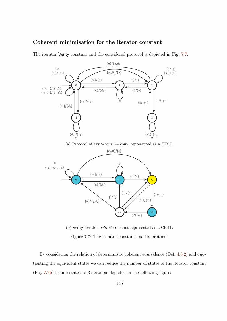
Coherent minimisation for the iterator constant
The iterator Verity constant and the considered protocol is depicted in Fig. 7.7.
0 1 2
34
∅{r2}/{d2}
{r2, n}/{q, d2}{r2, d1}/{r1, d2}
{r2}/{q}{r2,0}/{q}
{r2}/{r1} ∅
{0}/{}
{n}/{d2}
{0}/{q}{d1}/{r1}
{n}/{q, d2}
{}/{r1}{}/{q}
{d1}/{r1}∅
{d1}/{}
{d1}/{r1}∅
{d1}/{d2}
(a) Protocol of exp⊗ com1 ⊸ com2 represented as a CFST.
s4
s2s0 s1
s3
{0}/{}
{}/{r1}
{d1}/{}
{}/{q}{n}/{q, d2}
∅{r2, n}/{q, d2}
{r2}/{q}
{r2,0}/{q}
∅
{n}/{d2}
{d1}/{r1}{0}/{q}
(b) Verity iterator ’while’ constant represented as a CFST.
Figure 7.7: The iterator constant and its protocol.
By considering the relation of deterministic coherent equivalence (Def. 4.6.2) and quo-
tienting the equivalent states we can reduce the number of states of the iterator constant
(Fig. 7.7b) from 5 states to 3 states as depicted in the following figure:
145

s4
s2s0
∅
{r2, n}/{q, d2}
{n}/{d2}{r2}/{q}
{0}/{}{r2,0}/{q}
{}/{r1}
{d1}/{r1}{n}/{q, d2}{}/{q}
{0}/{q}{d1}/{}
However, if we consider Def. 4.4.4 for identifying the coherent equivalent states, then we
get optimised NCFST with only two states, as shown in the following figure:
s4s0
∅{r2, n}/{q, d2}{r2,0}/{q}
{n}/{d2}{r2}/{q}{0}/{} {}/{r1}
{d1}/{}{d1}/{r1}
{n}/{q, d2}{0}/{q}{}/{q}
Figure 7.8: Optimised Verity iterator ’while’ constant by coherent minimisation and con-sidering Def. 4.4.4.
7.2.1 Minimal CFSTs are not Unique
In Sec. 2.2.4 we have discussed that minimal DFSM is unique. In CFSTs, the minimisation
scenario is different. Because the coherent equivalence relation is intransitive and hence
more than one minimal CFST (with same number of states) can be obtained by the
coherent minimisation. For example, Fig. 7.9 shows an alternative possible minimal CFST
for the iterator Verity constant. In fact, this figure is functionally equivalent to Fig. 7.8
under the same protocol (Fig. 7.7a). The only difference between these two figures is that
146

in Fig. 7.8 state s2 is quotiented with the blue states in one state while in Fig. 7.9 state
s4 is combined with the set of blue states.
s2s0
{r2, n}/{q, d2}{n}/{q, d2}{n}/{d2}
{r2}/{q}{d1}/{}{}/{q}∅
{0}/{}{r2,0}/{q}{0}/{q}
{d1}/{r1}{}/{r1}
Figure 7.9: Another possible minimal Verity iterator ’while’ constant.
7.3 Symbolic Coherent Minimisation of Verity Con-
stants
In Sec. 5.3 we explained by example how the symbolic coherent minimisation can be
applied on SFSTs. In the following three figures we demonstrate that symbolic coherent
minimisation can optimise the constants of Verity language (represented in SFST model),
e.g. the binary addition constant. As we discussed in Sec. 2.6.3, the binary addition
constant in Verity involves six input and output events, which are: request for evaluating
the result q3, request for the first argument q1, request for the second argument q2, value of
the first argument n, value of the second argument m, and the final result n+m. From the
hardware point of view, each event is corresponding to one port in the interface. Fig. 7.10
shows the suggested interface for the addition constant. Note that, the symbols ’i1’, ’i2’,
and ’i3’ correspond to input ports while ’o1’, ’o2’, and ’o3’ denote the three output ports
in this particular order. In fact, these six ports consist of only control bits in the symbolic
protocol while in the case of processes (represented by SFSTs) they involve data and
control bits. As we explained in Ch. 5 every SFST is defined over a signature, denoted
147

by A, and A is a pair that shows the number of input and output ports respectively.
Consequently, the signature of the addition constant in SFST is A = (3,3).q3
i1q1
o1
ni2q2
o2
mi3o3
n+m
Figure 7.10: Input and output ports for the binary addition constant in Verity
0 1
3
2
⟨1,0,0⟩/⟨0,0,1⟩
⟨1,1,0⟩/⟨1,0,1⟩⟨1,0,1⟩/⟨0,1,1⟩
⟨1,0,0⟩/⟨1,0,0⟩
⟨1,1,0⟩⟨1,0,0⟩⟨1,0,1⟩/⟨0,1,0⟩
⟨0,1,0⟩/⟨1,0,1⟩⟨0,0,1⟩/⟨0,1,1⟩
⟨0,1,0⟩/⟨1,0,0⟩
⟨0,1,0⟩/⟨0,0,1⟩
⟨0,1,0⟩/⟨0,0,0⟩
⟨0,0,0⟩/⟨1,0,0⟩
⟨0,1,0⟩/⟨1,0,0⟩⟨0,0,1⟩/⟨0,1,0⟩
⟨0,0,0⟩/⟨0,1,0⟩⟨1,0,0⟩/⟨0,1,0⟩
⟨0,0,1⟩/⟨0,0,1⟩⟨0,0,1⟩/⟨0,0,0⟩
⟨0,0,1⟩⟨0,1,0⟩
Figure 7.11: Symbolic Protocol of exp1 ⊗ exp2 ⊸ exp3 represented as a SFST.
As we can see in Fig. 7.13, we minimised the original SFST (Fig. 7.12) from four states
to only one state by considering the symbolic protocol presented in Fig. 7.11; applying
Def. 5.3.5; and finally quotienting the equivalent states.
148

s0 s1
s3
s2
⟨1,0,0⟩/⟨1,0,0⟩
⟨1,1,0⟩/⟨1,0,0⟩read(n)r1 ∶= n
read(m)/write(r1 +m)⟨0,0,1⟩/⟨0,1,1⟩
⟨0,1,0⟩/⟨0,0,0⟩read(n)r1 ∶= n
⟨0,0,0⟩/⟨0,1,0⟩⟨0,0,1⟩/⟨0,0,1⟩read(m)/write(r1 +m)
Figure 7.12: Verity binary addition constant represented as a SFST.
s0
⟨1,0,0⟩/⟨1,0,0⟩
⟨1,1,0⟩/⟨1,0,0⟩read(n)r1 ∶= n
⟨0,1,0⟩/⟨1,0,1⟩read(m)/write(r1 +m)
⟨0,1,0⟩/⟨0,0,0⟩read(n)r1 ∶= n
⟨0,0,0⟩/⟨0,1,0⟩
read(m)/write(r1 +m)⟨0,0,1⟩/⟨0,0,1⟩
Figure 7.13: Optimised Verity binary addition constant by symbolic coherent minimisa-tion.
149

7.4 Discussion
In this chapter, we examined the application of the coherent minimisation on the Verity
constants. Two coherent minimisation results have been outlined for each constant: the
first one corresponds to the coherent equivalence relation and the second corresponds to
the coherent deterministic state equivalence. These results have been compared with the
bisimulation quotienting. We noticed from these results that most of the constants are
optimised to NCFSTs with only one state, except the iterator and the parallel composition
constants, which can be minimised to 2 and 4 states, respectively. We also found that
the Verity constants can be minimised to DCFSTs with an average of 50% states-space
reduction. Finally, we examined the application of coherent minimisation on the Verity
constants represented as SFSTs.
150

CHAPTER 8
Conclusion and Future Work
8.1 Conclusion
In this thesis, we introduced a new notion of equivalence between states of a transducer,
dubbed coherent equivalence. It is weaker than the usual notions of bisimulation, so it leads
to more states being identified as equivalent, leading to more aggressive optimisations. Its
key idea is that the behaviour of the environment is restricted by a notion of protocol, also
specified as a transducer: a restricted environment has a weaker power of discriminating
actions of an observed system, thus rendering more states equivalent.
Based on it, as an immediate application, we also proposed an efficient way to synthe-
sise tamper-proof hardware circuits from programs written in conventional programming
languages using the GoS methodology. In this scenario the protocol is simply the rules of
the semantic game.
We introduced a slightly modified transducer model, concurrent finite state trans-
ducer (CFST) and an associated symbolic representations which can be used to handle a
transducer with very large (or infinite) states. In both cases we give a (finite) trace inter-
pretation and we present two important operations (composition and intersection) which
151

can be used to construct a larger system from smaller components. These transducers are
synthesisable into electronic circuits via VHDL.
Ch. 4 is the main theoretical contribution, introducing the coherent equivalence re-
lation, which makes rigorous the intuition that only certain interactions are permitted,
which in turn makes the environment less discriminating, and leads to more states in the
system being equivalent. This new equivalence is interesting because it can be used to
aggressively optimise transducers by reducing the number of states, a technique which
we call coherent minimisation. Unsurprisingly, it outperforms conventional state reduc-
tion techniques based on bisimulation quotienting. In fact, in the worst scenario when
the protocol permits all interactions this notion of equivalence reduces to conventional
bisimulation so it can be seen as a generalisation of it. Conversely, in the other limiting
example of the protocol with no interactions (empty protocol), all states of the transducer
are equivalent and can be identified and hence the transducer will be minimised to one
state.
The main result of the chapter is soundness: if two coherently equivalent states in a
transducer are identified, no other transducer compliant with the protocol under which
coherent equivalence is determined can tell the difference. Formally, the intersection
between the original transducer and the observer is equal, under the protocol, with the
intersection between the quotiented transducer and the same observer.
The second result is showing that coherent minimisation is not only sound, but also
compositional, i.e. it is preserved by transducer composition. This important result allows
the coherent minimisation to be applied to any sub-component of a larger system without
affecting its general properties, including coherence equivalence itself.
With special consideration to hardware synthesis we point out that coherently min-
imising deterministic CFST will not guarantee that the output will be deterministic. A
modified coherent equivalence relation, coherent deterministic states equivalence has been
152

suggested to overcome the problem of output-nondeterminism. Finally, we presented a
standard algorithm that relies on the coherent equivalence relation to reduce the number
of states in any CFST.
Next, we suggested a refined model of transducers, symbolic finite states transducer
(SFST). SFSTs have the ability to model systems which involve quantities expressed as
numbers. In SFSTs several transitions from one source state to different target states
can be combined into a single transition controlled by a predicate (or guard). SFSTs use
two components to represent states: a finite set of control states and a finite set of reg-
isters, which have initial values that can be modified explicitly via symbolic expressions
(updates). All definitions from Ch. 4 lift in the standard way to SFSTs since their correct-
ness is not contingent on the set of states being finite. We demonstrated that any SFST
can be translated to infinite concurrent transducers by mapping the register values into
a concrete state. The key difference between CFSTs and SFSTs is in their computational
properties, which for the latter can be undecidable. For this reason we restrict the notion
of symbolic protocol to the order in which ports are activated, ignoring the values on the
ports. This restriction enables us to define the relation of symbolic coherent simulation
and thereby the symbolic coherent equivalence relation. Consequently, we proved that
symbolic coherent minimisation is sound and compositional by translating SFSTs to in-
finite concurrent transducers and using the notion of coherent equivalence of concurrent
transducers.
A motivating application is discussed in Ch. 6: how circuits produced by a higher-level
synthesis compiler with FFI support can be subjected to low-level attacks. Low level
attacks occur when the system can implement actions that violate the programming-
language abstractions. In particular, when the input-output behaviour of the environ-
ment, in which the circuit operates, can breach the protocol-like semantics of the language.
We then elaborated on that constraining the behaviour of the environment to only legal
153

traces is possible by taking advantage of the fact that all the legal interactions between a
circuit and its environment can be described by a finite state machine, and hence by a dig-
ital circuit. We concluded this chapter by demonstrating that efficient tamper-proofness
is achievable by restricting the synthesised circuit to interact with its environment via a
monitor which detects all illegal interactions, and makes a proper defensive approach, e.g.
reset or halt, if any tampering attempt occurs.
Finally, in Ch. 7, we examined the usefulness of the coherent minimisation by applying
the coherent minimisation on the Verity constants represented by CFSTs. We compared
the optimisation results of coherent minimisation with the conventional bisimulation quo-
tienting. We noticed that most of the Verity constants can be optimised to NCFSTs with
one state. Iterator and parallel constants are the only exception, where the number of
states of their CFSTs models have been reduced by 50%. Generating optimised DCFSTs
from the Verity constants has been investigated too, with an average return of 50% states
reduction. Then, we demonstrated that the coherent equivalence relation is intransitive
and hence it might be a case of obtaining more than one minimal CFST. We ended this
chapter by showing that the symbolic coherent minimisation can aggressively optimise
SFST models of the Verity constants.
8.2 Future Work
This thesis has established a novel approach to aggressively minimise transducers oper-
ating in restricted environments. Also it has suggested a framework for efficient tamper-
proof hardware compilation. Several aspects in our work would benefit from further study.
However, there are also many research avenues that can be developed from this thesis.
We highlight some of these in the following points.
154

Connections with Session Types
Session Types allow safe conversations (interactions) between processes-like types. These
interactions have to conform to a protocol specified by the session types [79, 39, 38]. It is
obvious that there are some appealing connections with session types. In particular, the
use of session type to enforce run-time behaviour is very similar to the way we enforce
lawful environment actions in order to prevent tampering. However, the technical details
and especially the mathematical formulation of these ideas using process calculi rather
than automata need to be studied. We leave them as open questions for future work.
Integrating coherent minimisation with GoS
GoS is a technique for hardware compilation to generate behavioural descriptions of digi-
tal circuits from conventional languages [49, 60, 61, 62]. GoS was the motivation for this
research, and it will obviously benefit from coherent minimisation. In fact the proof of cor-
rectness of GoS stops at the automata-level and the VHDL implementation is done in an
ad hoc fashion, because the automated derivation of the automata would be prohibitively
expensive. The current implementations incorporate some rudiments of coherent min-
imisation, but the current theoretical framework would allow a top-to-bottom proof of
correctness for the GoS compiler.
Applications of coherent minimisation
Coherent minimisation is, of course, not restricted to GoS, which is meant to serve as
motivation and illustration, but to any automata operating in restricted environments.
For example, APIs themselves can be enforced by a protocol, stipulating that functions
belonging to the API must be called in a particular order. Finding other relevant applica-
tion is to exploit this general framework could lead to unexpected optimisations for other
systems.
155

Coherent minimisation algorithm
The coherent minimisation algorithm (Lst.4.1), which is based on the coherent equivalence
relation, will guarantee the resulting transducer has fewer states than the original one.
However, there is no assurance that the quotiented transducer is truly minimal. For any
transducer T and coherent equivalence relation R ⊆ ST × ST , if we assumed that the
output of running our coherent minimisation algorithm is m partitions, i.e. the resulting
minimised transducer T ′ has m states, then T ′ is minimal if and only if with any other
coherent equivalence relation R′ ⊆ ST × ST the algorithm will not return partitions less
than m. Further direction is to write an efficient algorithm to find the “optimal” coherent
equivalence relation that guarantees a minimum number of states from our minimisation
algorithm.
Certification
Fredriksson and Ghica verified (a version of) our soundness results for coherent minimisa-
tion and compositionality of CFSTs coherence. The differences (outlined in Appendix D),
are formally and technically significant, but conceptually they are still well within the
framework of the thesis. For the future we consider both extending the formal Agda
proofs to non-deterministic and symbolic transducers, as in this thesis, as well as extend-
ing some of the certification towards the GoS front-end and the VHDL back-end.
Efficient tamper-proof compilation
Tamper-proofing is an approach for preventing low-level attacks on hardware circuits.
We suggested in this thesis a model for efficiently tamper-proofing circuits produced by
a higher-level synthesis compiler, which monitors (and then prevents) the interactions
that do not respect the programming language protocol. However, this suggested model
of tamper-proofing is not limited to this application, and should apply to other areas
156

outside the hardware synthesis, in particular seamless distributed computing [47]. This
distribution system operates under a protocol that restricts the interaction between the
connected nodes and also controls the data flow between its nodes. Because of these
reasons, any interaction that tries to exploit vulnerabilities in its distributed network can
be prevented by enforcing the rules of the protocol.
VHDL behavioural description of SFSTs
CFST is unsuitable in dealing with numerical data, due to the very large numbers of states
required. SFSTs have been introduced in this thesis to overcome these problems. In this
thesis we presented an algorithm for generating VHDL code from CFSTs. However, this
algorithm can be modified to also encode SFSTs, by considering the guards as a part
from the condition of the encoded transitions and introducing the registers as additional
signals which will be updated (according to the update function) within every clock cycle.
Furthermore, we need to encode the control bits which specify the status (active/inactive)
of the input/output ports, as we explained in Ch. 5. This is quite important in order to
fully certify the GoS chain of compilation.
157

158

Bibliography
[1] Martın Abadi. Protection in programming-language translations. In ICALP, pages868–883, 1998.
[2] Martin Abadi, Mihai Budiu, Ulfar Erlingsson, and Jay Ligatti. Control-flow in-tegrity principles, implementations, and applications. ACM Trans. Inf. Syst. Secur.,13(1), 2009.
[3] Amr T. Abdel-hamid, Mohamed Zaki, and Sofiene Tahar. A tool converting finitestate machine to vhdl. In Proceedings of IEEE Canadian Conference on Electrical& Computer Engineering (CCECE’04), Niagara Falls, 2004.
[4] Samson Abramsky. Semantics of interaction: an introduction to game semantics.In P. Dybjer and A. Pitts, editors, Proceedings of the 1996 CLiCS Summer School,Isaac Newton Institute, pages 1–31. Cambridge University Press, 1997.
[5] Samson Abramsky. Algorithmic game semantics: A tutorial introduction. InH. Schichtenberg and R. Steinbruggen, editors, Proceedings of the NATO AdvancedStudy Institute, Marktober- dorf, pages 21–47. Kluwer Academic Publishers, 2001.
[6] Samson Abramsky, Dan R. Ghica, Andrzej S. Murawski, and C.-H. Luke Ong.Applying game semantics to compositional software modeling and verification. InTACAS, pages 421–435, 2004.
[7] Samson Abramsky, Dan R. Ghica, Andrzej S. Murawski, and C. H Luke Ong.Applying game semantics to compositional software modelling and verification. InProceedings of TACAS 04, LNCS, pages 421–435. Springer-Verlag, 2004.
[8] Samson Abramsky and Guy McCusker. Game semantics. In Computational logic,pages 1–55. Springer, 1999.
159

[9] Rakesh Agrawal and Ramakrishnan Srikant. Privacy-preserving data mining. InProceedings of the 2000 ACM SIGMOD international conference on Managementof data, SIGMOD ’00, pages 439–450, New York, NY, USA, 2000. ACM.
[10] Roland Airiau, Jean-Michel Berge, and vincent Olive. Circuit Synthesis with VHDL.Kluwer Academic Publishers, 1994.
[11] Rajeev Alur and Thomas A. Hezinger. Reactive modules. Formal Methods In SystemDesign, 15:7–48, 1999.
[12] Paul Amblard, Fabienne Lagnier, and Michel Levy. Finite state machines: compo-sition, verification, minimization: a case study. In 10th International Conferenceon Mixed Design (MIXDES03), Lodz, Poland, 2003.
[13] Ross Anderson and Markus Kuhn. Tamper resistance-a cautionary note. In Pro-ceedings of the second Usenix workshop on electronic commerce, volume 2, pages1–11, 1996.
[14] Kumar Avijit, Prateek Gupta, and Deepak Gupta. Tied, libsafeplus: Tools forruntime buffer overflow protection. In USENIX Security Symposium, pages 45–55,2004.
[15] David F. Bacon, Susan L. Graham, and Oliver J. Sharp. Compiler transformationsfor high-performance computing. ACM Computing Surveys, 26, 1993.
[16] Adam Bakewell and Dan R Ghica. On-the-fly techniques for game-based softwaremodel checking. In Tools and Algorithms for the Construction and Analysis ofSystems, pages 78–92. Springer, 2008.
[17] Adam Bakewell and Dan R. Ghica. Compositional predicate abstraction from gamesemantics. In TACAS, pages 62–76, 2009.
[18] Clark W. Barrett, Roberto Sebastiani, Sanjit A. Seshia, and Cesare Tinelli. Sat-isfiability modulo theories. In Handbook of Satisfiability, volume 185, chapter 26,pages 825–885. IOS Press, 2009.
160

[19] Michael Ben-Or, Shafi Goldwasser, and Avi Wigderson. Completeness theoremsfor non-cryptographic fault-tolerant distributed computation. In Proceedings of thetwentieth annual ACM symposium on Theory of computing, STOC ’88, pages 1–10,New York, NY, USA, 1988. ACM.
[20] J. Bergandy, B. Mikolajckaz, and L. Beyga. Algebraic and Structural AutomataTheory. NORTH-HOLLAND Press, 1991.
[21] Jean Berstel, Luc Boasson, and Plivier Carton. Hopcroft’s automaton minimizationalgorithm and sturmian words. In Fifth Colloquium on Mathematics and ComputerScience, 2008.
[22] Gavin M. Bierman, Andrew D. Gordon, and David Langworthy. Semantic subtypingwith an smt solver. Technical report, Microsoft Research, 2010.
[23] Nikolaj Bjørner and Margus Veanes. Symbolic transducers. Technical report, Mi-crosoft Research, January 2011.
[24] Norbert Blum. An o(n log n) implementation of the standard method for minimizingn-state finite automata. Information Processing Letters, 57:65–69, 1996.
[25] Robert King Brayton, Alberto L. Sangiovanni-Vincentelli, Curtis T. McMullen,and Gary D. Hachtel. Logic Minimization Algorithms for VLSI Synthesis. KluwerAcademic Publishers, 1984.
[26] A. Brown. Optimising transformations for hardware compilation. Technical report,Department of Computing, Imperial College London, 2005.
[27] Stephen Brown and Zvonko Vranesic. fundamentals of digital logic with vhdl design.McGraw-Hill, 2005.
[28] Jan Cappaert and Bart Preneel. A general model for hiding control flow. In Pro-ceedings of the tenth annual ACM workshop on Digital rights management, pages35–42. ACM, 2010.
[29] Celoxica Limited. Handel-C: Language Reference Manual, 2005.
161

[30] Suresh Chari, Charanjit S Jutla, Josyula R Rao, and Pankaj Rohatgi. Towardssound approaches to counteract power-analysis attacks. In Advances in Cryptology,CRYPTO’99, pages 398 – 412. Springer, 1999.
[31] Kwang Ting Cheng and A. S. Krishnakumar. Automatic generation of functionalvectors using the extended finite state machine model. ACM Trans. on designAutomation of Electronic Systems, 1:57–79, 1996.
[32] Ben Cohen. VHDL coding styles and methodologies. Kluwer Academic Publishers,1999.
[33] David J Creasey. Advanced signal processing, volume 13. Iet, 1985.
[34] Clifford E. Cummings. State machine coding styles for synthesis. In SNUG’98(Synopsys Users Group San Jose, CA, 1998) Proceedings, 1998.
[35] Pierre-Louis Currien. Notes on game semantics. Technical report, Paris University,2006.
[36] Leonardo de Moura and Nikolaj Bjørner. Satisfiability modulo theories: An appe-tizer. In Formal Methods: Foundations and Applications, 12th Brazilian Symposiumon Formal Methods, SBMF 2009, Gramado, Brazil, August 19-21, 2009, Revised Se-lected Papers, volume 5902 of Lecture Notes in Computer Science. Springer, 2009.
[37] Leonardo Mendonca de Moura and Nikolaj Bjørner. Satisfiability modulo theories:introduction and applications. Commun. ACM, 54(9):69–77, 2011.
[38] Mariangiola Dezani-Ciancaglini, Dimitris Mostrous, Nobuko Yoshida, and SophiaDrossopoulou. Session types for object-oriented languages. In ECOOP 2006–Object-Oriented Programming, pages 328–352. Springer, 2006.
[39] Mariangiola Dezani-Ciancaglini, Nobuko Yoshida, Alexander Ahern, and SophiaDrossopoulou. A distributed object-oriented language with session types. In Trust-worthy Global Computing, pages 299–318. Springer, 2005.
[40] Aleksandar Dimovski, Dan R Ghica, and Ranko Lazic. Data-abstraction refinement:A game semantic approach. Springer, 2005.
162

[41] Aleksandar Dimovski, Dan R Ghica, and Ranko Lazic. A counterexample-guidedrefinement tool for open procedural programs. In Model Checking Software, pages288–292. Springer, 2006.
[42] Johan Ditmar and Steve McKeever. Function call optimisation in systemc hardwarecompilation. In Proceedings of Programmable Logic, 2008.
[43] Bruno Dutertre and Leonardo De Moura. The yices smt solver. Technical report,SRI International, 2006.
[44] Levent Erkok and John Matthews. Using Yices as an automated solver in Is-abelle/HOL. In Automated Formal Methods’08, Princeton, New Jersey, USA, pages3–13. ACM Press, 2008.
[45] Sebastian Faust, Krzysztof Pietrzak, and Daniele Venturi. Tamper-proof circuits:How to trade leakage for tamper-resilience. In Automata, Languages and Program-ming, pages 391–402. Springer, 2011.
[46] Jean-Claude Fernandez. An implementation of an efficient algorithm for bisimula-tion equivalence. Science of Computer Programming, 13(2):219–236, 1990.
[47] Olle Fredriksson and Dan R Ghica. Seamless distributed computing from the ge-ometry of interaction. Trustworthy Global Computing, 2012.
[48] Rosario Gennaro, Anna Lysyanskaya, Tal Malkin, Silvio Micali, and Tal Rabin. Al-gorithmic tamper-proof (atp) security: Theoretical foundations for security againsthardware tampering. In Theory of Cryptography, pages 258–277. Springer, 2004.
[49] Dan R. Ghica. Geometry of Synthesis: a structured approach to VLSI design. InPOPL, pages 363–375, 2007.
[50] Dan R. Ghica. Applications of game semantics: From program analysis to hard-ware synthesis. In Logic In Computer Science, 2009. LICS’09. 24th Annual IEEESymposium on, pages 17–26. IEEE, 2009.
[51] Dan R. Ghica. Function interface models for hardware compilation. In MEM-OCODE, pages 131–142, 2011.
163

[52] Dan R. Ghica and Zaid Al-Zobaidi. Coherent minimisation: Towards efficienttamper-proof compilation. EPTCS, 104:83–98, 2012.
[53] Dan R Ghica and Guy McCusker. Reasoning about idealized algol using regularlanguages. In Automata, Languages and Programming, pages 103–115. Springer,2000.
[54] Dan R Ghica and Guy McCusker. The regular-language semantics of second-orderidealized algol. Theoretical Computer Science, 309(1):469–502, 2003.
[55] Dan R. Ghica and Mohamed N. Meena. On the compositionality of round abstrac-tion. In CONCUR’10 Proceeding of the 21st international Conference on Concur-rency, 2010.
[56] Dan R. Ghica and Mohamed N. Menaa. Synchronous game semantics via roundabstraction. In FOSSACS, pages 350–364, 2011.
[57] Dan R Ghica and Andrzej S Murawski. Compositional model extraction for higher-order concurrent programs. Springer, 2006.
[58] Dan R. Ghica. and Andrzej S. Murawski. Angelic semantics of fine-grained concur-rency. Annals of Pure and Applied Logic, 151:89–114, 2008.
[59] Dan R. Ghica, Andrzej S. Murawski, and C.-H. Luke Ong. Syntactic control ofconcurrency. Theor. Comput. Sci., 350(2-3):234–251, 2006.
[60] Dan R. Ghica and Alex Smith. Geometry of Synthesis II: From games to delay-insensitive circuits. Electr. Notes Theor. Comput. Sci., 265:301–324, 2010.
[61] Dan R. Ghica and Alex Smith. Geometry of Synthesis III: Resource managementthrough type inference. In POPL, pages 345–356, 2011.
[62] Dan R. Ghica, Alex Smith, and Satnam Singh. Geometry of Synthesis IV: compilingaffine recursion into static hardware. In ICFP, pages 221–233, 2011.
164

[63] Dan R. Ghica and Nikos Tzevelekos. A system-level game semantics. ElectronicNotes in Theoretical Computer Science, 286:191–211, 2012.
[64] V. M. Glushkov. Automata theory and structural design problems of digital ma-chines. Cybernetics and Systems Analysis, 1:3–9, 1965.
[65] M. Gokhale, J. Stone, J. Arnold, and M. Kalinowski. Streams-oriented fpga com-puting in the streams-c high level language. In IEEE Symposium on FPGAs forCustom Computing Machines, 2000.
[66] Steve Golson. State machine design techniques for verilog and vhdl. SynopsysJournal of High-Level Design, 9:1–48, 1994.
[67] Sezer Goren and F. Joel Ferguson. On state reduction of incompletely specifiedfinite state machines. Computers and Electrical Engineering, 33(1):58 – 69, 2007.
[68] Sudhakar Govindavajhala and Andrew W Appel. Using memory errors to attack avirtual machine. In Security and Privacy, 2003. Proceedings. 2003 Symposium on,pages 154–165. IEEE, 2003.
[69] Z. Guo, B. Buyukkurt, and W. Najjar. Input data reuse in compiling windowoperations onto reconfigurable hardware. SIGPLAN Not., 39(7):249–256, 2004.
[70] Z. Guo, W. Najjar, and B. Buyukkurt. Efficient hardware code generation for fpgas.ACM Transactions on Architecture and Code Optimization, 5:1–26, 2008.
[71] Sumit Gupta. User Manual for the SPARK Parallelizing High-Level SynthesisFramework. Center for Embedded Computer Systems, University of California atSan Diego and Irvine, 2004.
[72] Sumit Gupta, Nikil Dutt, Rajesh Gupta, and Alexandru Nicolau. Spark: A high-level synthesis framework for applying parallelizing compiler transformations. In InInternational Conference on VLSI Design, 2003.
[73] Sumit Gupta, Nikil Dutt, Rajesh Gupta, and Alexandru Nicolau. Coordinatedparallelizing compiler optimizations and high-level synthesis. ACM Transactions onDesign Automation of Electronic Systems, 9:441–470, 2004.
165

[74] William Von Hagen. The Definitive Guide to GCC. Apress, 2004.
[75] Matthew Hague and C-H Luke Ong. Symbolic backwards-reachability analysis forhigher-order pushdown systems. In Foundations of Software Science and Computa-tional Structures, pages 213–227. Springer, 2007.
[76] Michael A. Harrison. Introduction to Formal Language Theory. Addison-WesleyLongman Publishing Co., Inc., 1978.
[77] Hiroyuki Higuchi and Yusuke Matsunaga. A fast state reduction algorithm forincompletely specified finite state machines. In Design Automation Conference Pro-ceedings 1996, 33rd, pages 463–466. IEEE, 1996.
[78] Hiroyuki Higuchi and Yusuke Matsunaga. A fast state reduction algorithm forincompletely specified finite state machines. In Design Automation Conference Pro-ceedings 1996, 33rd, pages 463–466. IEEE, 1996.
[79] Kohei Honda, Nobuko Yoshida, and Marco Carbone. Multiparty asynchronoussession types. In ACM SIGPLAN Notices, volume 43, pages 273–284. ACM, 2008.
[80] S. J. Hong, R. G. Cain, and D. L. Ostapko. Mini: A heuristic approach for logicminimization. IBM Journal of Research and Development, 18:443–458, 1974.
[81] John Hopcroft. An n log n algorithm for minimizing states in a finite automaton.Technical report, Stanford university, 1971.
[82] John E. Hopcroft, Rajeev Motwani, and Jeffrey D. Ullman. Introduction to Au-tomata Theory, Languages, and Computation. Addison-Wesley, 2001.
[83] Yuval Ishai, Manoj Prabhakaran, Amit Sahai, and David Wagner. Private circuitsii: Keeping secrets in tamperable circuits. In Advances in Cryptology-EUROCRYPT2006, pages 308–327. Springer, 2006.
[84] Yuval Ishai, Amit Sahai, and David Wagner. Private circuits: Securing hardwareagainst probing attacks. In Advances in Cryptology-CRYPTO 2003, pages 463–481.Springer, 2003.
166

[85] Helmut Jurgensen and Stavros Konstantinidis. Handbook of formal languages, vol.1: word, language, grammar. Springer-Verlag New York, Inc., 1997.
[86] Keil Software. Cx51 Compiler User’s Guide, 2001.
[87] G. M. Kelly and M. L. Laplaza. Coherence for compact closed categories. Journalof Pure and Applied Algebra, 19:193–213, 1980.
[88] Sunil P Khatri, Amit Narayan, Sriram C Krisnan, Kenneth L McMillan, Robert KBrayton, and A Sangiovanni-Vincentelli. Engineering change in a non-deterministicfsm setting. In Proceedings of the 33rd annual Design Automation Conference, pages451–456. ACM, 1996.
[89] Darko Kirovski, Milenko Drinic, and Miodrag Potkonjak. Engineering change pro-tocols for behavioral and system synthesis. Computer-Aided Design of IntegratedCircuits and Systems, 24(8):1145–1155, 2005.
[90] Timo Knutila. Re-describing an algorithm by hopcroft. Theortical Computer Sci-ence, pages 333–363, 2001.
[91] Sava Krstic and Amit Goel. Architecting solvers for sat modulo theories: Nelson-oppen with dpll. In Frontiers of Combining Systems, volume 4720 of Lecture Notesin Computer Science, pages 1–27. Springer Berlin Heidelberg, 2007.
[92] K. Kuusilinna, V. Lahtinen, T. Hamalainen, and J. Saarinen. Finite state machineencoding for vhdl synthesis. In Finite state machine encoding for VHDL synthesis,volume 148, pages 23–30, 2001.
[93] David Lee and Mihalis Yannakakis. Online minimization of transition systems (ex-tended abstract). In Proceedings of the twenty-fourth annual ACM symposium onTheory of computing, STOC ’92, pages 264–274. ACM, 1992.
[94] David Lie, Chandramohan Thekkath, Mark Mitchell, Patrick Lincoln, Dan Boneh,John Mitchell, and Mark Horowitz. Architectural support for copy and tamperresistant software. ACM SIGPLAN Notices, 35(11):168–177, 2000.
167

[95] W. M. Mckeeman. Peephole optimization. Communications of the ACM, 8:443–444,1965.
[96] Robin Milner. A calculus of communicating systems. Springer-Verlag New York,Inc., 1982.
[97] Robin Milner and Davide Sangiorgi. Barbed bisimulation. In Automata, Languagesand Programming, pages 685–695. Springer, 1992.
[98] Mehryar Mohri. Weighted finite-state transducer algorithms: An overview. InFormal Languages and Applications, volume volume 148. Springer, Berlin, 2004.
[99] Alan Mycroft and Richard Sharp. A statically allocated parallel functional language.In ICALP, pages 37–48, 2000.
[100] W. Najjar, B. Buyukkurt, and Z. Guo. Compiler optimization for configurableaccelerators. In Proceedings of Int. Workshop on Applied Reconfigurable Computing(ARC), 2006.
[101] Zainalabedin Navabi. VHDL: Analysis and Modeling of Digital Systems. McGraw-Hill, Inc., 1993.
[102] Vijay A. Nebhrajani and Nayan Suthar. Finite state machines: A deeper look intosynthesis optimization for vhdl. In 11th International Conference on VLSI Design,pages 516–521, 1998.
[103] Gertjan Van Noord and Dale Gerdemann. Finite state transducers with predicatesand identities. Grammars, 4(3):263–286, 2001.
[104] Peter W. O’Hearn, John Power, Makoto Takeyama, and Robert D. Tennent. Syn-tactic control of interference revisited. Theor. Comput. Sci., 228(1-2):211–252, 1999.
[105] Daniel Page. Theoretical use of cache memory as a cryptanalytic side-channel.Technical report, Citeseer, 2002.
168

[106] Jorge M. Pena and Arlindo L. Oliveira. A new algorithm for exact reduction ofincompletely specified finite state machines. Computer-Aided Design of IntegratedCircuits and Systems, IEEE Transactions on, 18(11):1619–1632, 1999.
[107] Alexandre Petrenko, Re Petrenko, Roland Groz, and Sergiy Boroday. Confirmingconfigurations in efsm testing. IEEE Transactions on Software Engineering, 30:29–42, 2004.
[108] Benjamin Pierce and Davide Sangiorgi. Typing and subtyping for mobile processes.In Logic in Computer Science, 1993. LICS’93., Proceedings of Eighth Annual IEEESymposium on, pages 376–385. IEEE, 1993.
[109] Benjamin C Pierce and Davide Sangiorgi. Behavioral equivalence in the polymorphicpi-calculus. Journal of the ACM (JACM), 47(3):531–584, 2000.
[110] Andrei Pun, Mihaela Pun, and Alfonso Rodrıguez-Paton. On the hopcroft’s mini-mization technique for dfa and dfca. Theortical Computer Science, 410(24-25):2424–2430, 2009.
[111] Nader I. Rafla and Brett LaVoy Davis. A study of finite state machine coding stylesfor implementation in fpgas. In Proceedings of the 49th IEEE International MidwestSymposium on Circuits and Systems, pages 337–341, 2006.
[112] Silvio Ranise and Cesare Tinelli. Intelligent systems and formal methods in softwareengineering. IEEE Intelligent Systems, 21(6):71–81, 2006.
[113] Mike Reape and Henry Thompson. Parallel intersection and serial composition offinite state transducers. In Proceedings of the 12th conference on Computationallinguistics, 1988.
[114] John C. Reynolds. Syntactic control of interference. In POPL, pages 39–46, 1978.
[115] John C. Reynolds. The essence of Algol. In Proceedings of the 1981 InternationalSymposium on Algorithmic Languages, pages 345–372. North-Holland, 1981.
[116] Elaine Rich. Automata, computability and complexity: theory and applications.Pearson Prentice Hall, 2008.
169

[117] Richard L. Rudell. Multiple-valued logic minimization for pla synthesis. Technicalreport, EECS Department, University of California, Berkeley, 1986.
[118] Matthew Sackman and Susan Eisenbach. Session types in haskell. 2008.
[119] Jacques Sakarovitch. Elements of Automata Theory. Cambridge University Press,2009.
[120] Davide Sangiorgi. On the origins of bisimulation and coinduction. ACM Transac-tions on Programming Languages and Systems (TOPLAS), 31(4):15, 2009.
[121] Hovav Shacham, Matthew Page, Ben Pfaff, Eu-Jin Goh, Nagendra Modadugu, andDan Boneh. On the effectiveness of address-space randomization. In ACM Confer-ence on Computer and Communications Security, pages 298–307, 2004.
[122] Thomas R. Shiple, James H. Kukula, and Rajeev K. Ranjan. A comparison ofpresburger engines for efsm reachability. In CAV, pages 280–292, 1998.
[123] Michael Sipser. Introduction to the Theory of Computation. THOMSON, secondedition, 2006.
[124] Synario Design Automation. VHDL Reference Manual, 1997.
[125] Takenaka Takashi, Okano Kozo, Higashino Teruo, and Taniguchi Kenichi. Symbolicmodel checking of extended finite state machines with linear constraints over integervariables. Systems and Computers in Japan, 37(6):64–72, 2006.
[126] T. Todman, W. Luk, and J. Coutinho. Customisable hardware compilation. Super-computing, 32:119–137, 2005.
[127] Margus Veanes, Nikolaj Bjørner, and Leonardo De Moura. Symbolic automataconstraint solving. In LPAR-17, volume 6397 of LNCS, pages 640–654. Springer,2010.
[128] Margus Veanes, Pieter Hooimeijer, Benjamin Livshits, David Molnar, and NikolajBjørner. Symbolic finite state transducers: algorithms and applications. In POPL,pages 137–150, 2012.
170

[129] Margus Veanes, David Molnar, and Benjamin Livshits. Decision procedures forcomposition and equivalence of symbolic finite state transducers. Technical report,Microsoft Research, 2011.
[130] Tiziano Villa. Encoding Problems in Logic Synthesis. PhD thesis, GRADUATEDIVISION of the UNIVERSITY of CALIFORNIA at BERKELEY, 1995.
[131] Tiziano Villa. Synthesis of Finite State Machines: Functional Optimization. KluwerAcademic Pub, 1997.
[132] Arcilio Virginia, Yana Yankova, and Koen. Bertels. An empirical comparison of ansi-c to vhdl compilers: Spark, roccc and dwarv. In Proceedings of Annual Workshopon Circuits, Systems and Signal Processing, pages 388–394, 2007.
[133] M. Weinhardt and W. Luk. Evaluating hardware compilation techniques. In Pro-ceedings of the IEEE Symposium on Field-Programmable Custom Computing Ma-chines, IEEE Comput. Soc, 2000.
[134] Niklaus Wirth. Hardware compilation: Translating programs into circuits. Com-puter, 31(6):25–31, 1998.
[135] Xilinx. Coding Style Guidelines.
[136] XILINX. Synthesis and Simulation Design Guide, 2010.
[137] Yingjie XU. Describing an n log n algorithm for minimizing states in deterministicfinite automaton. January 2009.
[138] Y. Yankova, K. Bertels, G. Kuzmanov, G. Gaydadjiev, Y. Lu, and S. Vassiliadis.Dwarv: Delftworkbench automated reconfigurable vhdl generator. In Proceedings ofthe 17th International Conference on Field Programmable Logic and Applications,2007.
[139] Yana Yankova, Koen Bertels, Stamatis Vassiliadis, Roel Meeuws, and Arcilio Vir-ginia. Automated hdl generation: Comparative evaluation. In Proceedings of Inter-national Symposium on Circuits and Systems (ISCAS2007), 2007.
171

172

APPENDIX A
VHDL Constructs
Listing A.1: Syntax of “If” Statement in VHDL.
IF condition 1 THEN
statements ;
ELSIF condition 2 THEN
statements ;
...
ELSE statements ;
END IF;
Listing A.2: Syntax of “Case” Statement in VHDL.
CASE control - expression IS
WHEN test - expression 1 => statements ;
WHEN test - expression 2 => statements ;
...
WHEN OTHERS => statements ;
END CASE ;
173

174

APPENDIX B
Behavioural Description of CFST
Listing B.1: VHDL Code of Fig. 3.5a.
library IEEE ;
use IEEE . std_logic_1164.all;
ENTITY CFST IS
PORT ( CLK , RESET , r, d1, d2 : IN std_logic ;
r1 , r2, d : OUT std_logic );
END CFST ;
ARCHITECTURE behavioural OF CFST IS
TYPE state_type IS (s0, s1, s2, s3);SIGNAL state: state_type ;
BEGIN
PROCESS (CLK ,RESET)
VARIABLE x_r1 , z_r2 , y_d: std_logic ;
BEGIN
x_r1 :=0; z_r2 :=0; y_d :=0;
175

IF RESET =’1’
THEN
state <= s0
ELSIF CLK = ’1’AND CLK ’EVENT
THEN
CASE state IS
WHEN s0 => IF (r= ’1’ AND d1=’0’ AND d2=’0’)
THEN
state <= s1;
x_r1 :=’1’;
ELSIF (r= ’1’ AND d1=’1’ AND d2=’0’)
THEN
state <= s2;
x_r1 :=’1’;
ELSE state <= s0;
END IF;
WHEN s1 => IF (r= ’0’AND d1=’1’ AND d2=’0’)
THEN
state <= s2;
ELSE
state <= s1;
END IF;
WHEN s2 =>
IF (r= ’0’AND d1=’0’ AND d2=’1’)
THEN
z_r2 :=’1’;
176

y_d := ’1’;
state <= s0;
ELSE
z_r2 :=’1’;
state <= s3;
END IF;
WHEN s3 => IF (r= ’0’AND d1=’0’ AND d2=’1’)
THEN
y_d := ’1’;
state <= s0;
ELSE
state <= s3;
END IF;
END CASE ;
END IF;
r1 <= x_r1 ; r2 <= z_r2 ; d <= y_d;
END PROCESS ;
END behavioral ;
177

178

APPENDIX C
Coherent Minimisation for Verity Constants
Table C.1: Coherent Minimisation for Verity Constants in Detail.
Incompatible states Coherent equivalent Coherent deterministic
state equivalent
Sequential s0 /≃ s2, s1 /≃ s2 s0 ≍ s1, s0 ≍ s3 all pairs
composition s2 /≃ s3 s1 ≍ s3
Assignment s0 /≃ s2, s1 /≃ s2 s0 ≍ s1, s0 ≍ s3 all pairs
s2 /≃ s3 s1 ≍ s3
Conditional s0 /≃ s2, s0 /≃ s3, s1 /≃ s2 s0 ≍ s1, s0 ≍ s4 all pairs
’if ’ s1 /≃ s3, s2 /≃ s3, s2 /≃ s4 s0 ≍ s5, s1 ≍ s4
s2 /≃ s5, s3 /≃ s4, s3 /≃ s5 s1 ≍ s5, s4 ≍ s5
Binary s0 /≃ s2, s1 /≃ s2 s0 ≍ s1, s0 ≍ s3 all pairs
addition s2 /≃ s3 s1 ≍ s3
Iterator s0 /≃ s2, s0 /≃ s4, s1 /≃ s2 s0 ≍ s1, s0 ≍ s3 all pairs
’while’ s1 /≃ s4, s2 /≃ s3, s2 /≃ s4 s1 ≍ s3 except
s3 /≃ s4 s2 /≍ s4
Dereferencing None s0 ≍ s1 s0 ≍ s1
Diagonal s1 /≃ s2 s0 ≍ s1, s0 ≍ s2 all pairs
Parallel s0 ≍ S, s1 ≍ {s3, s4, s5}
composition – s2 ≍ {s3, s4}, s3 ≍ {s5, s6} –
(NCFST) {s4, s5, s6} ≍ s7
The above table shows the relations of compatibility, coherent state equivalence and
the deterministic state coherent equivalence for Verity constants. These constants with
179

their corresponding protocols have been presented in Ch. 7 except the binary addition
and the assignment constants, which are presented in this appendix.
By comparing Fig. C.3 and Fig. C.2 we can observe that the binary operator constant
has been minimised to only two states, using the relation of coherent deterministic state
equivalence. Likewise, the assignment constant is optimised to two states as shown in
Fig. C.6.
0 1
3
2
∅{q3}/{k3}
{q3, n1}/{q1, k3}{q3,m2}/{q2, k3}
{q3}/{q1}
{q3, n1}/{q1}{q3,m2}/{q2}
{n1}/{q1, k3}{m2}/{q2, k3}
∅{q1}/{n1}
{n1}/{k3}
{n1}/{}
{}/{q1}
{n1}/{q1}{m2}/{q2}
{}/{q2}{q3}/{q2}
{m2}/{k3}{m2}/{}
{m2}/{q2}∅
Figure C.1: Protocol of exp1 ⊗ exp2 ⊸ exp3 represented as a CFST.
180

s0 s1
s3
s2
∅
{q3}/{q1}
{q3, n1}/{q1}
{m2}/{q2, k3}
∅
{n1}/{}
{}/{q2}{m2}/{k3}
∅
Figure C.2: Verity binary addition constant represented as a CFST.
s2s0
{q3}/{q1}
{q3, n1}/{q1}
{m2}/{q2;k3}
{n1}{}
{}/{q2}
∅{m2}/{k3}
Figure C.3: Optimised Verity binary addition operator constant by coherent minimisation.
181

0 1
3
2
∅{r2}/{d2}
{r2, n1}/{q1, d2}{r2, ok}/{wn, d2}
{r2}/{q1}
{r2, n1}/{q1}{r2, ok}/{wn}
{n1}/{q1, d2}{ok}/{wn, d2}
∅{q1}/{n1}
{n1}/{d2}
{n1}/{}
{}/{q1}
{n1}/{q1}{ok}/{wn}
{}/{wn}{r2}/{wn}
{ok}/{d2}{ok}/{}
{ok}/{wn}∅
Figure C.4: Protocol of var ⊗ exp1 ⊸ com2 represented as a CFST.
s0 s1
s3
s2
∅
{r2}/{q1}
{r2, n1}/{q1}
{ok}/{wn, d2}
∅
{n1}/{}
{}/{wn}{ok}/{d2}
∅
Figure C.5: Verity assignment constant represented as a CFST.
182

s2s0
{r2}/{q1}
{r2, n1}/{q1}
{ok}/{wn;d2}
{n1}{}
{}/{wn}
∅{ok}/{d2}
Figure C.6: Optimised Verity assignment constant by coherent minimisation.
183

184

APPENDIX D
Formal Proofs of Coherent Minimisation in Agda
Below is the contents of the module1 which proves two versions of the main results of the
thesis: soundness of coherent minimization and compositionality of transducer coherence.
Compared to the thesis, there are several differences:
• The results in the thesis are proved for non-deterministic transducers, whereas the
results here are proved for partially defined deterministic transducers. These are
formally simpler, hence the formal Agda proofs are simpler, but in terms of hardware
synthesis they are still a very good fit.
• The formulation of the properties are in terms of bisimulation between transducers
rather than equivalences between states of the same transducers. This formulation
turns out to be easier to work with.
These differences are formally and technically significant, but conceptually they are still
well within the framework of the thesis.
module PDTrans where
open import Data.Empty
1Agda code by Olle Fredriksson and Dan R. Ghica.
185
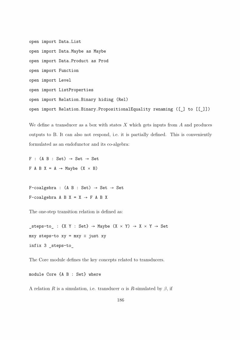
open import Data.List
open import Data.Maybe as Maybe
open import Data.Product as Prod
open import Function
open import Level
open import ListProperties
open import Relation.Binary hiding (Rel)
open import Relation.Binary.PropositionalEquality renaming ([_] to [[_]])
We define a transducer as a box with states X which gets inputs from A and produces
outputs to B. It can also not respond, i.e. it is partially defined. This is conveniently
formulated as an endofunctor and its co-algebra:
F : (A B : Set) → Set → Set
F A B X = A → Maybe (X × B)
F-coalgebra : (A B : Set) → Set → Set
F-coalgebra A B X = X → F A B X
The one-step transition relation is defined as:
_steps-to_ : {X Y : Set} → Maybe (X × Y) → X × Y → Set
mxy steps-to xy = mxy ≡ just xy
infix 3 _steps-to_
The Core module defines the key concepts related to transducers.
module Core {A B : Set} where
A relation R is a simulation, i.e. transducer α is R-simulated by β, if
186

_≤⟨_⟩_ : {X Y : Set} ( : F-coalgebra A B X) (R : Rel X Y)
( : F-coalgebra A B Y) → Set
≤⟨ R ⟩ = ∀ x y a → R x y → ∀ x’ b → x a steps-to (x’ , b) →
∃ y’ → y a steps-to (y’ , b) × R x’ y’
Correctness is defined relative to the conventional notion of (finite) trace semantics.
data _at_∋_ {X : Set} ( : F-coalgebra A B X) (x : X) : List (A × B)
→ Set where
: at x ∋ []
next : (a : A) (b : B) (x’ : X) {abs : List (A × B)}
→ x a steps-to (x’ , b) → at x’ ∋ abs → at x
∋ ((a , b) ∶∶ abs)
Two useful ancillary concepts is of trace membership and trace inclusion of transducers:
_∈_at_ : {X : Set} (t : List (A × B)) ( : F-coalgebra A B X) (x:X)
→ Set t ∈ at x = at x ∋ t
_at_⊑_at_ : {X Y : Set} ( : F-coalgebra A B X) (x : X)
( : F-coalgebra A B Y) (y : Y)
→ Set
at x ⊑ at y = ∀ {t} → t ∈ at x → t ∈ at y
Specific to our framework is the notion of inclusion under a given protocol (¶). Unlike
transducers, which are fully specified, protocols are only represented by their membership
predicate.
_⊢_at_⊑_at_ : {X Y : Set} (¶ : List (A × B) → Set)
( : F-coalgebra A B X) (x : X)
187

( : F-coalgebra A B Y) (y : Y) → Set
¶ ⊢ at x ⊑ at y = ∀ t t’ → ¶ (t ++ t’) → t’ ∈ at x → t’ ∈
at y
If a trace t is in the trace-set of a transducer we can define a transitive closure of the
next-step function, which is well defined.
_* : {X : Set} ( : F-coalgebra A B X) (x : X) {t : List (A × B)}
→ t ∈ at x → X
_* x = x
_* x (next a b x’ h h’) = ( *) x’ h’
The first main result is that our current definitions are sound, with simulation implying
trace inclusion. It is only a sanity result, not needed subsequently.
thm-sim-trace : {X Y : Set} ( : F-coalgebra A B X)
( : F-coalgebra A B Y)
(x : X) (y : Y) (R : Rel X Y) →
R x y → ≤⟨ R ⟩ → at x ⊑ at y
thm-sim-trace x y R r s =
thm-sim-trace x y R r s (next a b x’ h ih)
= next a b y’ h’ (thm-sim-trace x’ y’ R r’ s ih)
where
s’ : ∃ y’ → y a steps-to (y’ , b) × R x’ y’
s’ = s x y a r x’ b h
y’ = proj1 s’
r’ : R x’ y’
r’ = proj2 (proj2 s’)
h’ : y a steps-to (y’ , b)
188

h’ = proj1 (proj2 s’)
open Core
The definition below, preceded by some ancillary one, is that of interaction of two trans-
ducers. It is the synchronisation of the shared ports in B, but not followed by hiding.
maybeMap : {A B : Set} → (A → B) → Maybe A → Maybe B
maybeMap f = maybe (just ○ f) nothing
impos-maybe : {A : Set} (a : A) (b : Maybe A) → b ≡ nothing → just
a ≡ b → �
impos-maybe a nothing refl ()
_▶_ : {X Y A B C : Set} ( : F-coalgebra A B X) ( : F-coalgebra B C Y)
→ F-coalgebra A (B × C) (X × Y)
( ▶ ) (x , y) a = maybe ( {(x’ , b)
→ maybeMap (Prod.map (_,_ x’) (_,_ b)) ( y b)})
nothing ( x a)
Although obviously deterministic, we need to establish this formally for transducers using
propositional equality.
determinism : {X A B : Set}
( : F-coalgebra A B X) (x : X)(a : A){x1 x2 : X}{b1 b2 :B}
→ x a steps-to (x1 , b1) → x a steps-to (x2 , b2)
→ x1 ≡ x2 × b1 ≡ b2
determinism x a eq1 eq2 with x a
189

determinism x a refl refl | just (x’ , b’) = refl , refl
determinism x a () () | nothing
This helps us compose and especially de-compose a transducer interaction in terms of
the (unique) action on which they synchronize. This ancillary lemma would fail for non-
deterministic transducers, where it would be significantly more involved.
lem0 : {X Y A B C : Set} ( : F-coalgebra A B X) ( : F-coalgebra B C Y)
→ ∀ x1 y1 a → ∀ {x2 y2 b c} →
( ▶ ) (x1 , y1) a steps-to ((x2 , y2) , (b , c)) →
( x1 a steps-to (x2 , b)) × ( y1 b steps-to (y2 , c))
lem0 x1 y1 a h0 with x1 a
lem0 x1 y1 a h0 | just (x’ , b’) with y1 b’ | inspect ( y1) b’
lem0 x1 y1 a refl | just (x’ , b’) | just (y2’ , c’) | [[ r ]]
= refl , r
lem0 x1 y1 a () | just (b’ , x’) | nothing | [[ r ]]
lem0 x1 y1 a () | nothing
lem1 : {X Y A B C : Set}
( : F-coalgebra A B X) ( : F-coalgebra B C Y)
→ ∀ x1 y1 a b → ∀ {x2 y2 c} →
x1 a steps-to (x2 , b) → y1 b steps-to (y2 , c) →
( ▶ ) (x1 , y1) a steps-to ((x2 , y2) , (b , c))
lem1 x1 y1 a b h h’ with x1 a | y1 b | inspect ( y1) b
lem1 x1 y1 a b refl refl | just (x2 , .b) | just (y2 , c) | [[ r’ ]]
= cong (maybe _ nothing) r’
lem1 x1 y1 a b h () | just _ | nothing | _
lem1 x1 y1 a b () h’ | nothing | _ | _
190

An important result is that simulation is preserved by interaction. This is also a sanity-
check which is not subsequently needed.
thm-comp-sim : {X Y X’ Y’ A B C : Set}
( : F-coalgebra A B X ) ( : F-coalgebra B C Y)
(’ : F-coalgebra A B X’) (’ : F-coalgebra B C Y’)
(R : Rel X X’) (S : Rel Y Y’) →
≤⟨ R ⟩ ’ → ≤⟨ S ⟩ ’ → ( ▶ ) ≤⟨ R ×-REL S ⟩(’ ▶ ’)
thm-comp-sim ’ ’ R S sa sp (x1 , y1) (x1’ , y1’) a R×S (x2 , y2)
(b , c) h
= (x2’ , y2’) , (lem1 ’ ’ x1’ y1’ a b (proj1 prop4) (proj1 prop5) ,
(proj2 prop4 , proj2 prop5))
where
r : R x1 x1’
r = proj1 R×S
s : S y1 y1’
s = proj2 R×S
sa’ : x1 a steps-to (x2 , b) → ∃ x2’
→ (’ x1’ a steps-to (x2’ , b)) × (R x2 x2’)
sa’ = sa x1 x1’ a r x2 b
sp’ : y1 b steps-to (y2 , c) → ∃ y2’
→ (’ y1’ b steps-to (y2’ , c)) × (S y2 y2’)
sp’ = sp y1 y1’ b s y2 c
prop0 : x1 a steps-to (x2 , b) × y1 b steps-to (y2 , c)
prop0 = lem0 x1 y1 a h
prop1 : ∃ x2’ → (’ x1’ a steps-to (x2’ , b)) × (R x2 x2’)
191

prop1 = sa’ (proj1 prop0)
prop2 : ∃ y2’ → (’ y1’ b steps-to (y2’ , c)) × (S y2 y2’)
prop2 = sp’ (proj2 prop0)
prop3 = proj1 prop1
x2’ = proj1 prop1
y2’ = proj1 prop2
prop4 : (’ x1’ a steps-to (x2’ , b)) × (R x2 x2’)
prop4 = proj2 prop1
prop5 : (’ y1’ b steps-to (y2’ , c)) × (S y2 y2’)
prop5 = proj2 prop2
Protocols need to be prefix-closed, and it is useful to prove that trace interpretations of
transducers are also prefix-closed (pc(−)). It follows that the empty trace ǫ is always a
trace of any transducer.
tmpc-lemma : {A B X : Set}
(t : List (A × B)) ( : F-coalgebra A B X) (x : X) →
∀ t’ t’’ → t ≡ t’ ++ t’’ →
t ∈ at x → t’ ∈ at x
tmpc-lemma .t’’ x [] t’’ refl mem =
tmpc-lemma .((a , b) ∶∶ t’ ++ t’’) x ((a , .b) ∶∶ t’) t’’ refl
(next .a b x’ eq mem)
= next a b x’ eq IH
where
IH : at x’ ∋ t’
IH = tmpc-lemma (t’ ++ t’’) x’ t’ t’’ refl mem
traces-pc : {A B X : Set} (t : List (A × B)) ( : F-coalgebra A B X)
192

(x : X) → pc ( t → t ∈ at x)
traces-pc t x .(t2 ++ a ∶∶ []) t2 a refl mem = tmpc-lemma (t2 ∶∶r a)
x t2 [ a ] refl mem
traces-empty : {A B X : Set} ( : F-coalgebra A B X) (x0 : X)
→ [] ∈ at x0
traces-empty x0 =
This is the key definition of the thesis, expressed in term of partially-defined transduc-
ers, the existence of a coherent simulation between two transducers. The definition is
parametrised by the protocol ¶. It says that for any legal trace w, any legal extension of
that trace will preserve the simulation R.
_,_⊢_▷_ : {A B X Y : Set}
(¶ : List (A × B) → Set) -- protocol
(R : Rel X Y) -- relation
( : F-coalgebra A B X)
( : F-coalgebra A B Y) → Set
¶ , R ⊢ ▷ =
∀ x y a b x’ w → R x y → ¶ w →
x a steps-to (x’ , b) → ¶ (w ∶∶r (a , b)) → ∃ y’ →
y a steps-to (y’ , b) × R x’ y’
Our first new result is that if transducers α,α′ and β,β′ have coherent simulations, re-
spectively, under protocols ¶1 and ¶2 then their compositions have a coherent simulation,
by the product relation, under the composite protocol. The composite protocol is defined
by synchronisation on the shared component B:
193

thm-comp-coh-sim : {X Y X’ Y’ A B C : Set}
( : F-coalgebra A B X) ( : F-coalgebra B C Y)
(’ : F-coalgebra A B X’) (’ : F-coalgebra B C Y’)
(R : Rel X X’) (S : Rel Y Y’)
(¶1 : List (A × B) → Set) (¶2 : List (B × C) → Set)
(pc¶1 : pc ¶1)(pc¶2 : pc ¶2) →
¶1 , R ⊢ ▷ ’ → ¶2 , S ⊢ ▷ ’ →
(¶1 ◾▸ ¶2) , (R ×-REL S) ⊢ ( ▶ ) ▷ (’ ▶ ’)
thm-comp-coh-sim ’ ’ R S ¶1 ¶2 pc¶1 pc¶2 ▷’ ▷’ (x1 , y1)
(x1’ , y1’) a (b , c) (x2 , y2) w rs ¶1◾▸¶2w ▶xa
¶1◾▸¶2w[a,b]
= (x2’ , y2’) , (fact4 ,(proj2 (proj2 sims) , proj2 (proj2 sims)))
where
r : R x1 x1’
r = proj1 rs
s : S y1 y1’
s = proj2 rs
prop0 : ( x1 a steps-to (x2 , b)) × ( y1 b steps-to (y2 , c))
prop0 = lem0 x1 y1 a ▶xa
x1a = proj1 prop0
y1b = proj2 prop0
w|ab = Data.List.map (proj1 ○ assoc) w
w|bc = Data.List.map proj2 w
fact0 : Data.List.map (proj1 ○ assoc) (w ++ [ a , b , c ])
≡ w|ab ++ [ a , b ]
fact0 = map-distr-app (proj1 ○ assoc) w [ a , b , c ]
194

fact3 : Data.List.map proj2 (w ++ [ a , b , c ]) ≡ w|bc ++ [ b , c ]
fact3 = map-distr-app proj2 w [ a , b , c ]
fact1 : ¶1 (Data.List.map (proj1 ○ assoc) (w ++ [ a , b , c ]))
fact1 = proj1 (int-proj ¶1 ¶2 (w ++ [ a , b , c ]) ¶1◾▸¶2w[a,b])
fact2 : ¶2 (Data.List.map proj2 (w ++ [ a , b , c ]))
fact2 = proj2 (int-proj ¶1 ¶2 (w ++ [ a , b , c ]) ¶1◾▸¶2w[a,b])
-- ... : .X’ ( z → (’ x1’ a ≡ just (b , z)) ( _ → R x2 z))
sims = ▷’ x1 x1’ a b x2 w|ab r
(proj1 (int-proj ¶1 ¶2 w ¶1◾▸¶2w)) x1a (subst ¶1 fact0 fact1)
-- ... : .Y’ ( z → (’ y1’ b ≡ just (c , z)) ( _ → S y2 z))
sims = ▷’ y1 y1’ b c y2 w|bc s
((proj2 (int-proj ¶1 ¶2 w ¶1◾▸¶2w))) y1b (subst ¶2 fact3 fact2)
x2’ = proj1 sims
’x1’a : ’ x1’ a steps-to (x2’ , b)
’x1’a = proj1 (proj2 sims)
y2’ = proj1 sims
’y1’b : ’ y1’ b steps-to (y2’ , c)
’y1’b = proj1 (proj2 sims)
fact4 : (’ ▶ ’) (x1’ , y1’) a steps-to ((x2’ , y2’) , (b , c))
fact4 = lem1 ’ ’ x1’ y1’ a b ’x1’a ’y1’b
Another soundness result, used as a sanity check which is not really needed subsequently
is the fact that simulation between two transducers is preserved by the transitive closure
of their transition relation.
lem-sound : {A B X Y : Set}
(¶ : List (A × B) → Set) → (pc¶ : pc ¶) →
(R : Rel X Y) (x0 : X) (y0 : Y) (r : R x0 y0)
195

(w w’ : List (A × B)) (¶ww’ : ¶ (w ++ w’))
( : F-coalgebra A B X)
( : F-coalgebra A B Y)
(w’∈ : w’ ∈ at x0)
(w’∈ : w’ ∈ at y0) →
¶ , R ⊢ ▷ →
R (( *) x0 w’∈) (( *) y0 w’∈)
lem-sound ¶ pc¶ R x0 y0 r w [] ¶ww’ ▷ = r
lem-sound ¶ pc¶ R x0 y0 r w (.(a , b) ∶∶ w’) ¶wa,b∶∶w’
(next a b x’ eq’ w’∈) (next .a .b y’ eq w’∈) ▷ = IH
where
¶w : ¶ w
¶w = pc* ¶ pc¶ w ((a , b) ∶∶ w’) ¶wa,b∶∶w’
¶w[a,b]w’ : ¶ ((w ∶∶r (a , b)) ++ w’)
¶w[a,b]w’ = subst ¶ (sym (append-assoc w [ a , b ] w’)) ¶wa,b∶∶w’
¶w∶∶a,b : ¶ (w ∶∶r (a , b))
¶w∶∶a,b = pc* ¶ pc¶ (w ∶∶r (a , b)) w’ ¶w[a,b]w’
coh-xy’ : ∃ ( y’’ → ( y0 a steps-to (y’’ , b)) ( _ → R x’ y’’))
coh-xy’ = ▷ x0 y0 a b x’ w r ¶w eq’ ¶w∶∶a,b
y’’ = proj1 coh-xy’
coh’ : R x’ y’’
coh’ = proj2 (proj2 coh-xy’)
coh’’ : y0 a steps-to (y’’ , b)
coh’’ = proj1 (proj2 coh-xy’)
p3 : y’’ ≡ y’
p3 = sym (proj1 (determinism y0 a eq coh’’))
196

p1 : R x’ y’
p1 = subst (R x’) p3 coh’
IH : R (( *) x’ w’∈) (( *) y’ w’∈)
IH = lem-sound ¶ pc¶ R x’ y’ p1
(w ∶∶r (a , b)) w’ ¶w[a,b]w’ w’∈ w’∈ ▷
Finally, our main soundness result is that coherent simulation implies trace inclusion,
under the same protocol ¶.
thm-sound : {A B X Y : Set}
(¶ : List (A × B) → Set)(pc¶ : pc ¶) →
(R : Rel X Y) (x0 : X) (y0 : Y) (r : R x0 y0)
( : F-coalgebra A B X)
( : F-coalgebra A B Y) →
¶ , R ⊢ ▷ →
¶ ⊢ at x0 ⊑ at y0
thm-sound ¶ pc¶ R x0 y0 r ¶,R⊢▷ w [] ¶wt t∈ =
thm-sound ¶ pc¶ R x0 y0 r ¶,R⊢▷ w ((.a , .b) ∶∶ abs) ¶wt
(next a b x’ e’’ t∈) with x0 a | inspect ( x0) a | y0 a |
inspect ( y0) a
thm-sound ¶ pc¶ R x0 y0 r ¶,R⊢▷ w ((.a , .b) ∶∶ abs) ¶wt
(next a b x’ e’’ t∈) | just (x’’ , b’’) | [[ e ]]
| just (y’ , b’’’) | [[ y’’’ ]] = next a b y’ y’ IH
where
p0 : (w ++ (a , b) ∶∶ []) ++ abs ≡ w ++ (a , b) ∶∶ abs
197

p0 = append-assoc w ((a , b) ∶∶ []) abs
¶w : ¶ w
¶w = pc* ¶ pc¶ w ((a , b) ∶∶ abs) ¶wt
¶w[a,b] : ¶ (w ∶∶r (a , b))
¶w[a,b] = pc* ¶ pc¶ (w ∶∶r (a , b)) abs (subst ¶ (sym p0) ¶wt)
fact : ∃ ( y’’ → ( y0 a steps-to (y’’ , b)) ( _ → R x’ y’’))
fact = ¶,R⊢▷ x0 y0 a b x’ w r ¶w (trans e e’’) ¶w[a,b]
y’’ = proj1 fact
y’’ : y0 a steps-to (y’’ , b)
y’’ = proj1 (proj2 fact)
y’’≡y’ : y’’ ≡ y’
y’’≡y’ = proj1 (determinism y0 a y’’ y’’’)
y’ : y0 a steps-to (y’ , b)
y’ = subst ( y’ → y0 a steps-to (y’ , b)) y’’≡y’ y’’
Rx’y’ : R x’ y’
Rx’y’ = subst (R x’) y’’≡y’ (proj2 (proj2 fact))
IH : at y’ ∋ abs
IH = thm-sound ¶ pc¶ R x’ y’ Rx’y’ ¶,R⊢▷ (w ∶∶r (a , b)) abs
(subst ¶ (sym p0) ¶wt) t∈
thm-sound ¶ pc¶ R x0 y0 r ¶,R⊢▷ w ((.a , .b) ∶∶ abs) ¶wt
(next a b x’ e’’ t∈) | just (x’’ , b’’) | [[ e ]]
| nothing | [[nothing ]] = �-elim contradiction
where
¶w : ¶ w
¶w = pc* ¶ pc¶ w ((a , b) ∶∶ abs) ¶wt
198

¶w[a,b] : ¶ (w ∶∶r (a , b))
¶w[a,b] = pc* ¶ pc¶ (w ∶∶r (a , b)) abs (subst 
(sym (append-assoc w ((a , b) ∶∶ []) abs)) ¶wt)
fact : ∃ ( y’ → ( y0 a steps-to (y’ , b)) ( _ → R x’ y’))
fact = ¶,R⊢▷ x0 y0 a b x’ w r ¶w (trans e e’’) ¶w[a,b]
y’ = proj1 fact
just : y0 a steps-to (y’ , b)
just = proj1 (proj2 fact)
¬nothing≡just : ∀ {A : Set}{a : A} → nothing ≡ (Maybe A ∋ just a) → �
¬nothing≡just ()
contradiction : �
contradiction = ¬nothing≡just (trans (sym nothing) just)
thm-sound ¶ pc¶ R x0 y0 r ¶,R⊢▷ w ((.a , .b) ∶∶ abs) ¶wt
(next a b h () t∈) | nothing | [[ e ]] | o’ | [[ e’ ]]
The following module contains properties of prefix-closed sets of traces required by the
main module.
module ListProperties where
open import Relation.Binary hiding (Rel)
open import Relation.Binary.PropositionalEquality hiding ([_])
open import Data.Empty
open import Data.List
open import Data.List.Properties
open import Data.Nat
open import Data.Product as Prod hiding (map)
199

open import Function
import Level
pc : {A : Set} → (List A → Set) → Set
pc m = ∀ l l’ a → l ≡ l’ ∶∶r a → m l → m l’
sc : {A : Set} → (List A → Set) → Set
sc m = ∀ l l’ a → l ≡ a ∶∶ l’ → m l → m l’
rev : {A : Set} → List A → List A
rev [] = []
rev (x ∶∶ l) = rev l ∶∶r x
append-neut-r : {A : Set} → (l : List A) → l ++ [] ≡ l
append-neut-r [] = refl
append-neut-r (x ∶∶ xs) = cong (_∶∶_ x) (append-neut-r xs)
append-assoc : {A : Set} → (x y z : List A) → ((x ++ y) ++ z)
≡ (x ++ (y ++ z))
append-assoc [] y z = refl
append-assoc (x ∶∶ xs) y z = cong (_∶∶_ x) (append-assoc xs y z)
rev-append-distr : {A : Set} → (l l’ : List A) → rev (l ++ l’)
≡ (rev l’) ++ (rev l)
rev-append-distr [] l’ = sym (append-neut-r (rev l’))
rev-append-distr (x ∶∶ l) l’ = p2
200

where
IH : rev (l ++ l’) ≡ (rev l’) ++ (rev l)
IH = rev-append-distr l l’
p0 : rev (l ++ l’) ++ x ∶∶ [] ≡ ((rev l’) ++ (rev l)) ++ x ∶∶ []
p0 = cong ( w → w ++ x ∶∶ []) IH
p1 : ((rev l’) ++ (rev l)) ++ x ∶∶ [] ≡ (rev l’) ++ (rev l) ++ x ∶∶ []
p1 = append-assoc (rev l’) (rev l) (x ∶∶ [])
p2 : rev (l ++ l’) ++ x ∶∶ [] ≡ (rev l’) ++ (rev l) ++ x ∶∶ []
p2 = trans p0 p1
rev-invo : {A : Set} → (l : List A) → rev (rev l) ≡ l
rev-invo [] = refl
rev-invo (x ∶∶ l) = trans p0 p1
where
IH : rev (rev l) ≡ l
IH = rev-invo l
p0 : rev (rev l ++ x ∶∶ []) ≡ x ∶∶ (rev (rev l))
p0 = rev-append-distr (rev l) (x ∶∶ [])
p1 : x ∶∶ (rev (rev l)) ≡ x ∶∶ l
p1 = cong ( w → x ∶∶ w) IH
map-all : {A B : Set} → (List A → Set) → (A → B) → (List B → Set)
map-all L f l = ∃ l’ → L l’ → l ≡ map f l’
rev-all : {A : Set} → (List A → Set) → (List A → Set)
rev-all L l = L (rev l)
201

prop-pc-rev : {A : Set} → (L : List A → Set) → pc L → sc (rev-all L)
prop-pc-rev L pcL .(a ∶∶ l’) l’ a refl h = pcL (rev l’ ++ a ∶∶ [])
(rev l’) a refl h
sc* : {A : Set} → (m : List A → Set) → (sc m) → (t t’ : List A) →
m (t ++ t’) → m t’
sc* m h [] t’ h’ = h’
sc* m h (x ∶∶ t) t’ h’ = IH
where
IH : m t’
IH = sc* m h t t’ (h (x ∶∶ t ++ t’) (t ++ t’) x refl h’)
sc-lemma : {A : Set} → (m : List A → Set) → (sc m) → (t : List A) →
m t → (m [])
sc-lemma m scm t h = sc* m scm t [] (subst m (sym (append-neut-r t)) h)
pc-lemma : {A : Set} → (m : List A → Set) → (pc m) → (t : List A) →
m t → (m [])
pc-lemma m pcm t mt = sc-lemma (rev-all m) scm’ (rev t) p1
where
scm’ : sc (rev-all m)
scm’ = prop-pc-rev m pcm
p2 : t ≡ rev (rev t)
p2 = sym (rev-invo t)
p1 : m (rev (rev t))
202

p1 = subst m p2 mt
pc* : {A : Set} → (m : List A → Set) → (pc m) → (t t’ : List A) →
m (t ++ t’) → m t
pc* m pcm t t’ mtt’ = subst m (rev-invo t) p1
where
-- can this be done in a less boring way?
m’ = rev-all m
scm’ : sc m’
scm’ = prop-pc-rev m pcm
p0 : ∀ t0 t1 → m’ (t0 ++ t1) → m’ t1
p0 t0 t1 h = sc* m’ scm’ t0 t1 h
p2 : rev (rev t’ ++ rev t) ≡ (rev (rev t)) ++ (rev (rev t’))
p2 = rev-append-distr (rev t’) (rev t)
p4 : t ≡ rev (rev t)
p4 = sym (rev-invo t)
p4’ : t’ ≡ rev (rev t’)
p4’ = sym (rev-invo t’)
p3 : (rev (rev t)) ++ (rev (rev t’)) ≡ t ++ t’
p3 = sym (cong2 _++_ p4 p4’)
p5 : t ++ t’ ≡ rev (rev t’ ++ rev t)
p5 = sym (trans p2 p3)
p6 : m (rev (rev t’ ++ rev t))
p6 = subst m p5 mtt’
p1 : m (rev (rev t))
p1 = p0 (rev t’) (rev t) p6
203

-- quotient a set of sequences by a prefix
_∖_ : {A : Set} → (m : List A → Set) (w : List A) (l : List A) → Set
(m ∖ w) l’ = ∀ l → l ≡ w ++ l’ → m l
quotient-pc : {A : Set} → (m : List A → Set) (w : List A)
→ (pc m) → pc (m ∖ w)
quotient-pc m w pcm .(l’ ++ a ∶∶ []) l’ a refl h .(w ++ l’) refl = pc*
m pcm (w ++ l’) [ a ] (subst m p2 (h (w ++ l’ ++ a ∶∶ []) refl))
where
p2 : w ++ l’ ++ [ a ] ≡ (w ++ l’) ++ [ a ]
p2 = sym (append-assoc w l’ (a ∶∶ []))
p1 : w ++ l’ ++ [ a ] ≡ w ++ l’ ++ [ a ]
p1 = refl
p0 : m (w ++ l’ ++ a ∶∶ [])
p0 = h (w ++ l’ ++ [ a ]) p1
Rel : Set → Set → Set1
Rel X Y = REL X Y Level.zero
-- pointwise product of relations
_×-REL_ : {X X’ Y Y’ : Set} → Rel X Y → Rel X’ Y’ → Rel (X × X’)
(Y × Y’) (R ×-REL S) (x , x’) (y , y’) = R x y × S x’ y’
assoc : {A B C : Set} → A × B × C → (A × B) × C
assoc (a , (b , c)) = (a , b) , c
204

-- interaction of two alphabets
_◾▸_ : {A B C : Set} → (List (A × B) → Set) → (List (B × C) → Set)
→ (List (A × B × C) → Set)
_◾▸_ {A} {B} {C} P Q w = (P (map proj1 (map assoc w)))
× (Q (map proj2 w))
assoc-map : {A B C : Set} (f : A → B) (g : B → C) (l : List A) →
map g (map f l) ≡ map (g ○ f) l
assoc-map f g [] = refl
assoc-map f g (x ∶∶ xs) = cong (_∶∶_ (g (f x))) (assoc-map f g xs)
map-distr-app : {A B : Set} (f : A → B) (l l’ : List A) →
map f (l ++ l’) ≡ map f l ++ map f l’
map-distr-app f [] ys = refl
map-distr-app f (x ∶∶ xs) ys = cong (_∶∶_ (f x)) (map-distr-app f xs ys)
int-proj : {A B C : Set} (P : List (A × B) → Set)
(Q : List (B × C) → Set) (w : List (A × B × C)) →
((P ◾▸ Q) w) → (P (map (proj1 ○ assoc) w)) × (Q (map proj2 w))
int-proj P Q w PQw rewrite assoc-map assoc proj1 w = PQw
-- inverse map on nil and unit list
nilmap : {A B : Set} (noas : List A) (f : A → B) → (map f noas ≡ [])
→ noas ≡ []
205

nilmap [] _ eq = refl
nilmap (_ ∶∶ _) _ ()
unitmap : {A B : Set} (b : B) ([a] : List A) (f : A → B) →
[ b ] ≡ map f [a] → ∃ a → [a] ≡ [ a ] × f a ≡ b
unitmap b [] f ()
unitmap b (a ∶∶ as) f eq = a , fact’’ , sym (proj1 fact)
where
fact : b ≡ f a × [] ≡ map f as
fact = ∶∶-injective eq
fact’ : as ≡ []
fact’ = nilmap as f (sym (proj2 fact))
fact’’ : a ∶∶ as ≡ a ∶∶ []
fact’’ = cong ( as → a ∶∶ as) fact’
-- prefix closure preserved by composition
int-pref-comp : {A B C : Set} → (P : List (A × B) → Set)
(Q : List (B × C) → Set) →
pc P → pc Q → pc (P ◾▸ Q)
int-pref-comp P Q pcP pcQ .(l’ ++ (a , b , c) ∶∶ []) l’ (a , b , c)
refl (h1 , h2) = goal1 , goal2
where
projab = abc → (proj1 abc , proj1 (proj2 abc)) ,
proj2 (proj2 abc)
206

l1 = (map proj1 (map projab l’))
l1’ = (map (proj1 ○ projab) l’)
l1≡l1’ : l1 ≡ l1’
l1≡l1’ = assoc-map projab proj1 l’
l1ab=l1’ab : l1 ++ [ a , b ] ≡ l1’ ++ [ a , b ]
l1ab=l1’ab = cong ( l → l ++ [ a , b ]) l1≡l1’
l2 = (map proj1 (map projab (l’ ++ (a , b , c) ∶∶ [])))
l2’ = (map (proj1 ○ projab) (l’ ++ [ a , b , c ]))
l2≡≡l2’ : l2 ≡ l2’
l2≡≡l2’ = assoc-map projab proj1 (l’ ++ [ a , b , c ])
eqab : l2’ ≡ l1’ ++ [ a , b ]
eqab = map-distr-app (proj1 ○ projab) l’ [ a , b , c ]
goal1 : P l1
goal1 = pcP l2 l1 (a , b) (trans l2≡≡l2’ (trans eqab
(sym l1ab=l1’ab))) h1
m = map proj2 l’
m’ = map proj2 (l’ ++ (a , b , c) ∶∶ [])
eqbc : m’ ≡ m ++ [ b , c ]
eqbc = map-distr-app proj2 l’ [ a , b , c ]
goal2 : Q (map proj2 l’)
goal2 = pcQ m’ m (b , c) eqbc h2
207