2-Layer Crossing Minimisation

Johan van Rooij

Overview

Problem definitions NP-Hardness proof Heuristics & Performance Practical Computation

One layer: ILP, Branch & Cut Two layer: local search

Crossing Number

The number crossings for a bipartite graph only depends on the ordering of the vertices in both layers.

So for a bipartite graph G=(V0,V1,E) and two orderings x0 of V0 and x1 of V1 we can compute the crossing number: cr(G,x0,x1)

Problem Definitions

One-sided two layer crossing minimisation problem: Given a graph and a fixed ordering x0

of V0, find an ordering x1 of V1 such that cr(G,x0,x1) is as small as possible.

Two-sided two layer problem: Given a graph find two orderings x0 of

V0 and x1 of V1 such that cr(G,x0,x1) is as small as possible.

NP-Hardness

We are going to prove NP-Hardness of the one-sided problem.

Two-sided problem also is NP-Hard. For this we prove the decision

problem NP-Complete: Given a graph G, ordering x0 of V0,

and integer M, is there and ordering x1 of V1 such that: cr(G,x0,x1) ≤ M ?

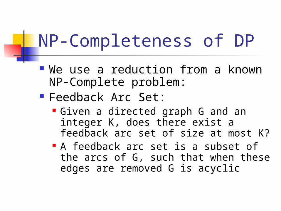
NP-Completeness of DP We use a reduction from a known

NP-Complete problem: Feedback Arc Set:

Given a directed graph G and an integer K, does there exist a feedback arc set of size at most K?

A feedback arc set is a subset of the arcs of G, such that when these edges are removed G is acyclic

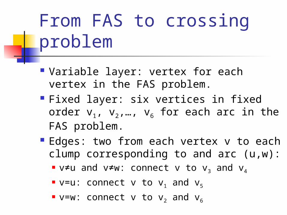
From FAS to crossing problem

Variable layer: vertex for each vertex in the FAS problem.

Fixed layer: six vertices in fixed order v1, v2,…, v6 for each arc in the FAS problem.

Edges: two from each vertex v to each clump corresponding to and arc (u,w): v≠u and v≠w: connect v to v3 and v4

v=u: connect v to v1 and v5

v=w: connect v to v2 and v6

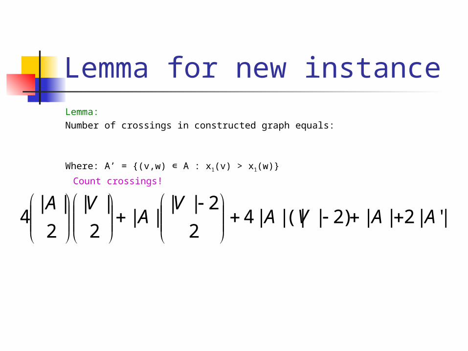
Lemma for new instanceLemma:Number of crossings in constructed graph equals:

Where: A’ = {(v,w) ∊ A : x1(v) > x1(w)}

Count crossings!

|'|2||)2|(|||42

2||||

2

||

2

||4 AAVA

VA

VA

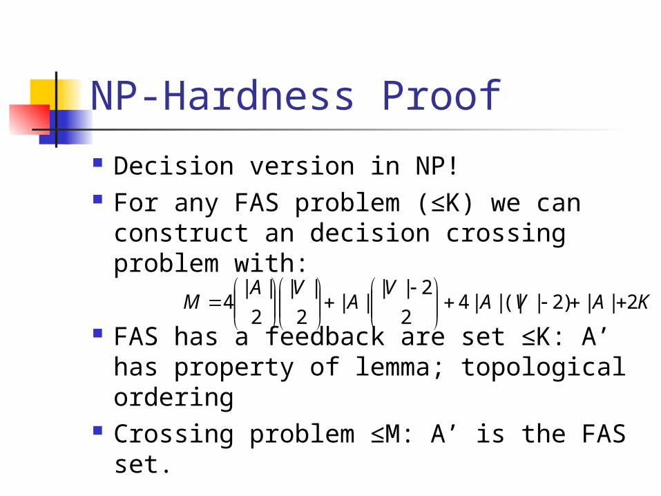
NP-Hardness Proof

Decision version in NP! For any FAS problem (≤K) we can

construct an decision crossing problem with:

FAS has a feedback are set ≤K: A’ has property of lemma; topological ordering

Crossing problem ≤M: A’ is the FAS set.

KAVAV

AVA

M 2||)2|(|||42

2||||

2

||

2

||4

Heuristics

Barycenter Heuristic Median Heuristic Penalty Minimisation Heuristic Assignment Heuristic

Performance of the Heuristics

Barycenter Heuristic

One of the first and still one of the best.

Given the ordering of the fixed layer x0, place the vertices at positions 1,2…

The Barycenter is the average of the positions of connected vertices.

Compute Barycenters of vertices in variable layer and place according to increasing barycenters.

Barycenter heuristic for two-sided problem.

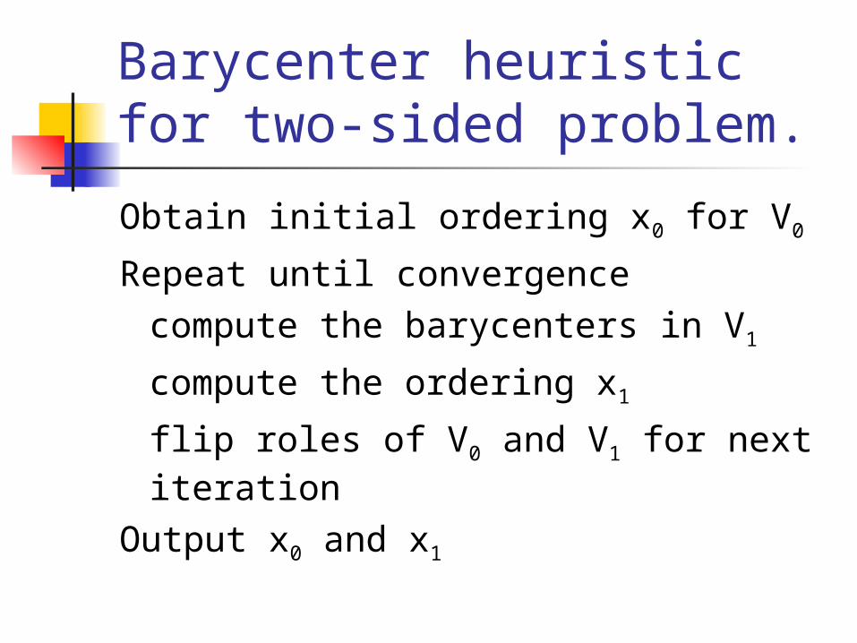
Obtain initial ordering x0 for V0

Repeat until convergencecompute the barycenters in V1

compute the ordering x1

flip roles of V0 and V1 for next iteration

Output x0 and x1

Properties of the Barycenter

Li and Stallman proved an approximation ratio d-1 for the one-sided problem

Where d is the maximum degree of a vertex in the variable layer

Although not indicated by the above: the barycenter performs better on dense graphs compared to sparse

Median Heuristic

The median heuristic is very much alike to the barycenter heuristic.

We now do not compute barycenters, but we compute medians to place the vertices in the variable layer

Eades and Wormald proved an performance ratio of 3. Or when there are more than cn2 edge a ratio of:

2

2

1

3

c

c

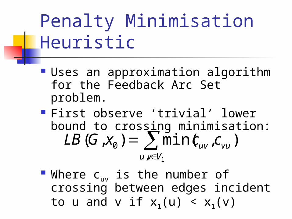
Penalty Minimisation Heuristic Uses an approximation algorithm

for the Feedback Arc Set problem. First observe ‘trivial’ lower bound

to crossing minimisation:

Where cuv is the number of crossing between edges incident to u and v if x1(u) < x1(v)

1,

0 ),min(),(Vvu

vuuv ccxGLB

Penalty Digraph

It may be clear that this lower bound can not always be obtained: The minimum chooses a vertex before

another, but these choices can contradict. Penalty digraph: directed graph which

captures these choices: cuv – cvu edges from v to u Cycle is a contradiction Find minimum FAS to obtain topological

sort

Approximation ratioof the PM-Heuristic

Solution of FAS problem to the penalty digraph directly relates to the number of crossings: sol(crossmin) = LB(G,x0) + sol(FAS)

Demetrescu and Finocchi show an approximation ratio equal to the longest simple cycle found in graph This extends to the crossing

minimisation problem

The Assignment Heuristic

Also a very popular heuristic Does not take edges from other

vertices into account, but all possible edges

Uses the O(n3) solvable assignment problem: Assign n items to n positions with minimal

cost where for each item-position combination we have cost cij (cost matrix)

Construction of the cost matrix

For each vertex and position construct the full bipartite graph and insert the vertex at that position, with edges to connected vertices in the original graph.

Number of crossings in this graph is upper bound for real number of crossings, we use this for the cost.

From the minimal cost assignment we obtain the positions of the vertices.

Performace

Hard to say which heuristic is better. One sided problem (random graphs)

Barycenter best Assignment next Median slightly worse

PM varies much in performance Depends too much on graphs used

by the different researchers.

Performace

Two sided problem (random graphs) Barycenter again the best But almost equal to the median heuristic Assignment worse

Barycenter and Median very fast to compute

Assignment and Penalty Minimisation slower

Practical Computation

Heuristics were the first approaches introduced by the literature

Heuristics are very nice for very large instances because of limited computation time

For smaller instances we can do significantly better.

For both problems we will show this

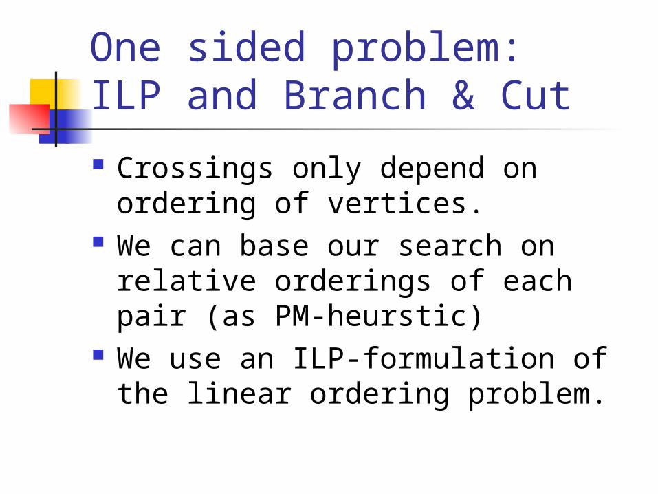
One sided problem:ILP and Branch & Cut

Crossings only depend on ordering of vertices.

We can base our search on relative orderings of each pair (as PM-heurstic)

We use an ILP-formulation of the linear ordering problem.

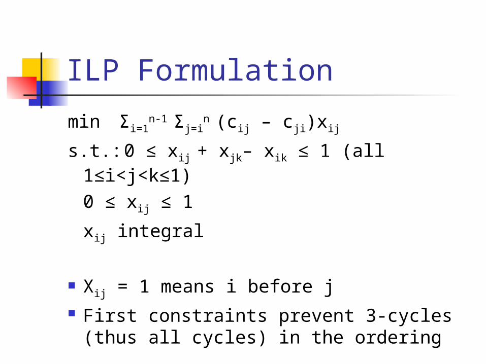
ILP Formulation

min Σi=1n-1 Σj=i

n (cij – cji)xij

s.t.: 0 ≤ xij + xjk– xik ≤ 1 (all 1≤i<j<k≤1)

0 ≤ xij ≤ 1

xij integral

Xij = 1 means i before j First constraints prevent 3-cycles (thus

all cycles) in the ordering

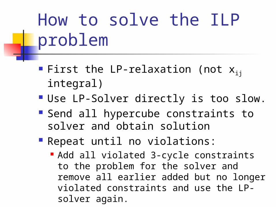
How to solve the ILP problem

First the LP-relaxation (not xij integral) Use LP-Solver directly is too slow. Send all hypercube constraints to

solver and obtain solution Repeat until no violations:

Add all violated 3-cycle constraints to the problem for the solver and remove all earlier added but no longer violated constraints and use the LP-solver again.

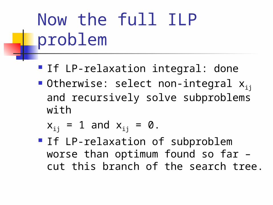
Now the full ILP problem

If LP-relaxation integral: done Otherwise: select non-integral xij and

recursively solve subproblems withxij = 1 and xij = 0.

If LP-relaxation of subproblem worse than optimum found so far – cut this branch of the search tree.

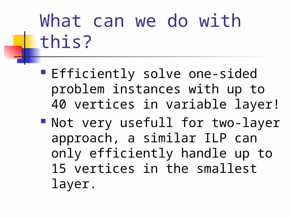
What can we do with this?

Efficiently solve one-sided problem instances with up to 40 vertices in variable layer!

Not very usefull for two-layer approach, a similar ILP can only efficiently handle up to 15 vertices in the smallest layer.

So what do we do for the two-layer problem?

The best solutions are obtained by means of local search.

In our survey we briefly explain an algorithm based on GRASP (Greedy RAndomised Search Procedure) and Path Relinking

Not in the scope of this presentation to explain this in more detail

Conclusion The 2-layer crossing minimisation is

important for other crossing minimisation problems

NP-Hard so no algorithm known that can compute the optimum in polynomial time

Many heuristics proposed with approximation ratios with often good performance

Practical computations of one-sided problem with ILP and Branch & Cut

For the two-layer problem: local search

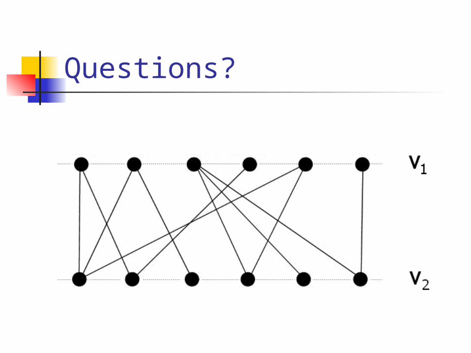
Questions?