coherence properties of supercontinuum generated …
TRANSCRIPT

COHERENCE PROPERTIES OF SUPERCONTINUUM GENERATED IN
HIGHLY NONLINEAR PHOTONIC CRYSTAL FIBERS
A dissertation
submitted by
Yuji Zhang
In partial fulfillment of the requirements
for the degree of
Doctor of Philosophy
In
Physics
TUFTS UNIVERSITY
February 2015
ADVISOR:
Prof. Fiorenzo G. Omenetto Tufts University, Department of Physics and Astronomy
and Department of Biomedical Engineering
RESEARCH COMMITTEE:
Prof. Peggy Cebe Tufts University, Department of Physics and Astronomy
Dr. Daniel J. Kane Mesa Photonics, LLC, Santa Fe, NM
Prof. Anthony W. Mann Tufts University, Department of Physics and Astronomy
Prof. Austin Napier Tufts University, Department of Physics and Astronomy
Prof. Krzysztof Sliwa Tufts University, Department of Physics and Astronomy
Prof. Roger G. Tobin Tufts University, Department of Physics and Astronomy

ii
This page is intentionally left blank.

iii
ACKNOWLEDGEMENTS
I would like to first of all thank my advisor Professor Fiorenzo Omenetto for his financial
support, academic guidance, and also his help in experiment and in writing. Without
those I would not have made my progress in research. He is so acute and fast in thinking,
and discussing with him and listening to his discussion is the best part of the training I
received in the graduate school. Looking at his bench work and his lab notebook, I saw a
perfect example of a precise, careful, and neat style, which I have been trying to mimic.
His influence on me has been more than just in research. He illustrates such a passionate
and indulgent attitude in work, just like his words: “It’s not about here (pointing to his
head) – it’s all about here (pointing to his heart).” It has been my privilege to work with
him and learn science and beyond.
I would like to thank my committee members. Dr. Daniel Kane has been so kind to share
his expertise and insights. I call him every several weeks and always benefit from his
advice. Professor Roger Tobin gave me lessons about writing, presentation, and also
generally about research. He read my thesis draft in short time and gave revision and
comments before my defense, so that I could improve my defense based on this feedback.
Professor William Oliver and Professor Krzysztof Sliwa spent their time to listen to my
trial defense and gave me advice on presentation, especially about how to make it
interesting to broader audience. As my academic advisor, Professor Krzysztof Sliwa
helped in my academic and personal life in my first a few years in the States. Professor
William Oliver sent me to ESL class. In those early days in the States when I was not so
comfortable and confident, their help was invaluable. Professor Anthony Mann is the

iv
person I always have casual talks with and learn from. Professor Peggy Cebe shared with
me very useful tips about organizing and managing research. Professor Austin Napier
revised my thesis so carefully and even found a missing paper in the reference. I feel
lucky to have such smart and kind committee members who are willing to share and help.
My labmates are fun to work with and also helpful. Dr. Jason Amsden was my mentor
when I started working in the lab. He shared his techniques and experience to get me
started. Without his help, it would have taken me longer to figure out the hands-on
techniques he taught me. Late Dr. Peter Domachuk also shared with me his expertise and
experience. Dr. Jessica Mondia and Mr. Jason Bressner gave me good suggestions about
research and about personal life. Dr. Hu “Tiger” Tao and Ms. Miaomiao “Mia” Tao have
deep understanding about research, and I often discussed with them about the stories of
papers. Mr. Matthew Applegate helped me a lot in writing. Writing in second language
English has been challenging for me. I always ask him for help in revision. He probably
has read my journal papers ten times. Other labmates are also nice to discuss with and
willing to help, including Dr. Giovanni Perotto, Dr. Sunghwan Kim, Dr. Jana
Kainerstorfer, Dr. Benedetto Marelli, Dr. Konstantinos Tsioris, Dr. Elijah Shirman, Mr.
Alex Mitropoulos, Mr. Mark Brenckle, Mr. Jonas Osorio, and Mr. Joshua Spitzberg.
I also want to thank Professor David Kaplan and Dr. Guokui Qin in Department of
Biomedical Engineering and Professor Subhas Kundu from Indian Institute of
Technology Kharagpur for opportunities to collaborate, so that I could have chances to
work with interesting rare materials and produce some publications. Dr. Martin Hunter in
Department of Biomedical Engineering and my friends Dr. Robert Stegeman and Dr.

v
Guang-ming “Derek” Tao are experts in relevant fields. I often talk to them and benefit
from the discussions.
Staff are sometimes less visible than professors, but are really indispensible. Ms. Milva
Ricci, Ms. Keleigh Sanford, and Ms. Carmen Preda in Department of Biomedical
Engineering and Ms. Gayle Grant, Ms. Shannon Landis-Amerault, Ms. Jacqueline
DiMichele, and Ms. Jean Intoppa in Department of Physics and Astronomy helped me
with all kinds of support. Mr. Scott MacCorkle and Mr. Denis Dupuis in the machine
shop made me gadgets that made experiments easy and fun.
My parents Jianfa Zhang and Meifeng Fan Zhang always have so much love for me.
They provided an atmosphere of study where I developed a will of pursuing more and
deeper knowledge. And they have been so supportive during the years when I am away
from them. My girlfriend Mengyi Liao is a pretty and smart girl. She has been supportive
and also giving me good suggestions. I owe a lot of thanks and love to them.

vi
This page is intentionally left blank.

vii
ABSTRACT
In this dissertation, experimentally measured spectral and coherence evolution of
supercontinuum (SC) is presented. Highly nonlinear soft-glass photonic crystal fibers
(PCF) were used for SC generation, including lead-silicate (Schott SF6) PCFs of a few
different lengths: 10.5 cm, 4.7 mm, and 3.9 mm, and a tellurite PCF of 2.7 cm. The pump
is an optical parametric oscillator (OPO) at 1550 nm with pulse energy in the order of
nanojoule (nJ) and pulse duration of 105 femtosecond (fs). The coherence of SC was
measured using the delayed-pulse method, where the interferometric signal was sent into
an optical spectrum analyzer (OSA) and spectral fringes were recorded. By tuning the
pump power, power-dependent evolution of spectrum and coherence was obtained.
Numerical simulations based on the generalized nonlinear Schrödinger equation
(GNLSE) were performed. To match the measured data, the simulated spectral evolution
was optimized by iteratively tuning parameters and comparing features. To further match
the simulated coherence evolution with the measurement, shot noise and pulse-to-pulse
power fluctuation were added in the pump, and the standard deviation of the fluctuation
was tuned.
Good agreement was obtained between the simulated and the measured spectral
evolution, in spite of the unavailability of some physical parameters for simulation. It is
demonstrated in principle that, given a measured spectral evolution, the fiber length, and
the average power of SC, all other parameters can be determined unambiguously, and the
spectral evolution can be reproduced in the simulations. Most importantly, the soliton fission
length can be simulated accurately.

viii
The spectral evolution using the 4.7- and the 3.9-mm SF6 PCFs shows a pattern
dominated by self phase modulation (SPM). This indicates that, these fiber lengths are
close to the soliton fission length at the maximum power. The spectral evolution using
the 10.5-cm SF6 PCF and the 2.7-cm tellurite PCF shows a soliton-fission-dominated
pattern, indicating these lengths are much longer than the soliton fission length at the
maximum power.
For the coherence evolution using the SF6 PCFs, the simulations and the measurements
show qualitative agreement, confirming the association between coherence degradation
and soliton fission. For the case of the tellurite PCF, nearly quantitative agreement is
shown, and it is shown that the solitonic coherence degrades slower than the overall
coherence.
Fluctuation of coherence occurs at the regime where the coherence starts to degrade, in
the measurement and the simulations of the SF6-PCF case. It is shown that the cause is
the pulse-to-pulse power fluctuation in the pump.
The pulse-to-pulse stability of spectral intensity is another characterization of SC
stability, other than the coherence. It is shown by simulations that these two exhibit
different dynamics, and have low correlation.

ix
TABLE OF CONTENTS
ACKNOWLEDGEMENTS ............................................................................................... iii
ABSTRACT ...................................................................................................................... vii
TABLE OF CONTENTS ................................................................................................... ix
LIST OF TABLES ............................................................................................................ xii
LIST OF FIGURES ......................................................................................................... xiii
LIST OF APPENDICES .................................................................................................. xix
ABBREVIATIONS AND ACRONYMS ......................................................................... xx
1. INTRODUCTION .......................................................................................................... 1
2. SUPERCONTINUUM GENERATION AND COHERENCE ...................................... 4
2.1 Photonic Crystal Fiber ............................................................................................... 5
2.2 Modeling of Supercontinuum Generation ................................................................. 6
2.2.1 The generalized nonlinear Schrödinger equation ............................................... 6
2.2.2 The dispersion term .......................................................................................... 11
2.2.3 The Raman term ............................................................................................... 14
2.2.4 Implementation of numerical simulation .......................................................... 21
2.3 Major Physical Processes in Supercontinuum Generation ...................................... 22
2.3.1 Kerr effect and self phase modulation .............................................................. 22
2.3.2 Dispersion ......................................................................................................... 23

x
2.3.3 Soliton and soliton fission ................................................................................ 26
2.3.4 Intrapulse Raman scattering ............................................................................. 29
2.3.5 Dispersive wave (Cherenkov radiation) generation ......................................... 31
2.4 Measurement of Coherence ..................................................................................... 32
2.4.1 Coherence of quasi-monochromatic light ......................................................... 32
2.4.2 Coherence of broadband light........................................................................... 35
2.4.3 Coherence of SC ............................................................................................... 37
3. BACKGROUND .......................................................................................................... 39
3.1 Simulation Research of SC Coherence ................................................................... 40
3.2 Experimental Research of SC Coherence ............................................................... 46
3.3 My Research ............................................................................................................ 50
4. METHODS ................................................................................................................... 51
4.1 Experiment .............................................................................................................. 52
4.2 Simulation ............................................................................................................... 57
4.2.1 Introduction ...................................................................................................... 57
4.2.2 The dispersion term .......................................................................................... 58
4.2.3 The Raman term ............................................................................................... 60
4.2.4 Simulation parameters ...................................................................................... 63
4.2.5 Modeling noise and coherence ......................................................................... 64
5. RESULTS AND DISCUSSIONS ................................................................................. 69

xi
5.1 Results Using SF6 PCFs ......................................................................................... 70
5.1.1 Experimental results ......................................................................................... 70
5.1.2 Simulated spectral evolution and discussions .................................................. 73
5.1.3 Simulated coherence and discussions ............................................................... 82
5.1.4 Conclusions ...................................................................................................... 89
5.2 Using Tellurite PCF ................................................................................................ 90
5.2.1 Experimental data ............................................................................................. 90
5.2.2 Simulated spectral evolution and discussions .................................................. 91
5.2.3 Simulated coherence evolution and discussions ............................................... 95
5.2.4 Conclusions ...................................................................................................... 99
6. CONCLUSIONS AND OUTLOOK .......................................................................... 101
REFERENCES ............................................................................................................... 104
APPENDIX A. SYSTEMATIC CHECK OF NUMERICAL SIMULATIONS ............ 109
APPENDIX B. PARAMETERS FOR SIMULATIONS IN SECTION 2.3 ................... 110
APPENDIX C. COMPUTER CODE FOR DATA PROCESSING AND NUMERICAL
SIMULATIONS ............................................................................................................. 111

xii
LIST OF TABLES
2.1 Comparison of media for supercontinuum (SC) generation.
2.2 Brief derivation of the generalized nonlinear Schrödinger equation (GNLSE).
2.3 Definition of the variables and the parameters in the GNLSE.
3.1 Summation of previous simulation research and their theories.
3.2 Key facts of previous experimental research on SC coherence.
4.1 Parameters of the PCFs and the pump used in the experiment, in comparison with
a silica PCF and a SF6 PCF in literature.
4.2 Polynomial fitting of the β2(ω−ω0) curve for the 3.6-μm-core SF6 PCF.
4.3 Polynomial fitting of the β2(ω−ω0) curve for the tellurite PCF.
4.4 Comparison of two Raman gain spectra: 1Rg reported in [Plotnichenko et al.,
2005] and 2Rg reported in [Stegeman et al., 2006; Qin et al., 2007; Yan et al.,
2010], and calculation of the Raman term.
4.5 Values of parameters for simulation (subject to change in the optimization
process).
B.1 Parameter values for each simulation in Fig. 2.1 and 2.2.

xiii
LIST OF FIGURES
2.1 Spectral and temporal evolution when different GVD is added to SPM. (a) SPM +
normal GVD. The normal GVD limits the spectral broadening. (b) SPM +
anomalous GVD. The pulse swings back and forth between spectrally-broader-
temporally-shorter and spectrally-narrower-temporally-longer. This is a higher-
order soliton propagating periodically (see Section 2.3.3). (c) SPM + a particular
value of anomalous GVD such that they perfectly balance each other. In this case
the pulse keeps invariant in spectrum and in temporal profile. This is a
fundamental soliton (see Section 2.3.3).
2.2 (a) Adding the Raman term causes soliton fission. The spectral trajectory and
temporal trajectory of a soliton are marked. The soliton fission length Lfiss = 0.48
cm is marked with white arrows. It can be seen this distance is where the pulse
reaches the maximum spectral width and the shortest duration before splitting,
which is consistent with this empirical definition of soliton fission length. (b)
Further adding 3rd-order dispersion causes dispersive wave (Cherenkov radiation)
in addition to soliton fission. The dispersive wave is marked in spectral and
temporal evolution.
2.3 Experiments of coherence measurement. (a) Young’s double slit experiment, and
(b) Michelson interferometry.
2.4 Methods to measure frequency-dependent coherence for broadband light. (a)
Interference of broadband light yields overlapped fringes of all frequencies. (b)
Spectrally resolve the signal along the direction of fringes (here vertically) to
obtain a 2D pattern. At horizontal line is the fringe of a frequency. (c) Spectrally
resolve the fringes in the direction perpendicular to the fringes (here horizontally),
resulting in a spectrum with fringes. Prisms are used to conceptually illustrate
spectrally resolving the signal.
3.1 Simulation results of SC coherence, excerpted from [Dudley et al., 2006]. (a) and
(b): Spectral and coherence evolution using a 100-fs and a 150-fs pump,
respectively. The pump peak power is 10 kW. The ZDW of the PCF is 780 nm,
and the pump wavelength is 835 nm (anomalous GVD pump). (c) Contour plot of
average coherence as a function of the pump wavelength and the pump pulse
duration. The pump peak power is fixed to be 4 kW. The ZDW of the PCF is 780
nm (marked with a dash line). (d) Average coherence vs. soliton number N,
summarized from multiple simulations using various parameter sets, in which the

xiv
pump wavelength is ranged 790–900 nm, pump pulse duration is 30–200 nm, and
pump peak power is 3–30 kW.
3.2 Simulated SC and its coherence, excerpted from [Türke et al., 2007]. A 410-fs
pump at 775 nm was used, and the pump peak powers are (a) 0.09 kW, (b) 0.9
kW, and (c) 5.9 kW. The fiber length is 9 cm. The authors argued that in the case
of (c), the MI-induced sidebands are weak when soliton fission happens, and the
ejected solitons are coherent.
4.1 SEM picture of the cross section of the highly nonlinear SF6 PCF. Inset is a close-
up of the core. The core diameter is 3.6 µm.
4.2 Microstructure and the dispersion of the Tellurite PCF. (a) Cross section of the
fiber under an optical microscope. (b) and (c) are closeups of the core under SEM
and under an optical microscope, respectively. (d) is the dispersion curve. The
ZDW is 1380 nm. These figures are excerpted from [Domachuk et al., 2008].
4.3 Experimental setup for the measurement of SC coherence.
4.4 1-mm SF6 PCF mounted on a customized stage using tape.
4.5 Calculation of the dispersion of the SF6 PCF. (a) Calculating the dispersion curve
of the 3.6-μm-core PCF based on the dispersion curves of a 2.6-μm and a 4-μm-
core SF6 PCFs, through linear interpolation. The 2.6-μm and the 4-μm-core
curves are excerpted from [Kumar et al., 2002]. (b) Linear curve fitting of
β2(ω−ω0)|3.6-μm.
4.6 Raman response function hR(t) of SF6. It is modeled as Eq. 2.2.61, with 1τ = 5.5
fs, 2τ = 32 fs, and fR = 0.13.
4.7 (a) Raman gain spectra gR(ω) of tellurite glasses. The green curve gR1 was
reported in [Plotnichenko et al., 2005], and the blue curve gR2 was reported in
[Stegeman et al., 2006; Qin et al., 2007; Yan et al., 2010]. Both are calibrated for
pump wavelength λ0 = 514.5 nm. (b) Raman response function hR(t) calculated
based on gR2, using Eq. 2.2.57.
5.1 Spectral evolution (a)–(c) and coherence evolution (d)–(f) of SC generated in
three different lengths of SF6 PCFs (10.5-cm, 4.7-mm, and 3.9-mm). The red
arrows in (a) mark soliton trajectories. The green arrow in (b) marks the
Cherenkov peak. The spectral evolution is calibrated such that the maximum
intensity is 0 dB. The lower limit of the color bar is set to −40 dB so that the 40-

xv
dB bandwidth is visualized in the evolution; the upper limit is set for optimal
visualization of features. (g)–(i) are line plots of representative spectra.
5.2 (a)–(c) Experimentally measured spectral evolution using three different lengths
of SF6 PCF, respectively. (d)–(f) Corresponding simulation results. The vertical
black line at 1700 nm helps visually comparing with the experimental data. (g)
and (h): Simulated spectral and temporal evolution depending on the propagation
length. P = 77 mW is used. It is shown graphically that soliton fission happens at
~9 mm. Analytically calculated soliton fission length is similar Lfiss = 10.2 mm. (i)
GVD D(λ) of the fiber. The red lines mark the zero dispersion wavelength (ZDW)
and the pump wavelength (1550 nm). The ZDW is ~1370 nm. The GVD at the
pump wavelength is ~38 ps/(nm∙km).
5.3 Determining the duration of the pump pulses. Red curve: measured output
spectrum at P = 2 mW and Lfiber = 3.9 mm. Black curves: simulated output
spectrum using a pump of transform-limited sech2 pulses of TFWHM = 100, 110,
and 120 fs, respectively. P = 2 mW and Lfiber = 3.9 mm are used.
5.4 Optimization of the simulated spectral evolution. Each line includes four plots of
spectral evolution: the beginning (low power) part of the 10.5-cm-fiber case, the
10.5-cm-fiber case, the 4.7-mm-fiber case, and the 3.9-mm-fiber case. (a)
Experimental data. (b) Simulations with TFWHM = 105 fs has been applied. (c)
Simulations after further tuning P to 1.3*P and γ to 1.38*γ. (d) Simulations after
further tuning β2(ω) to 2*β2(ω).
5.5 Simulated spectral evolution with varying initial chirps, in the case of the 4.7-mm
SF6 PCF. Adding positive or negative initial chirps causes features in the spectra,
and changes the power at which soliton fission happens. Emergence of the
Cherenkov peak is marked with red lines to represent the powers at which soliton
fission happens.
5.6 Comparison between (a) the measured spectral evolution and (b)–(d)
corresponding simulations using varying initial chirps, for the case of the 3.9-mm
SF6 fiber. (a) shows gaps (marked with arrows) between the central peak and the
spectral lobes. (b) and (c) also have these gaps, while in (d) a positive chirp (C =
0.1) flattens the central parts of the spectrum and causes the gaps to disappear.
Spectra at P = 40 mW are stacked in (e) to show the features clearly.
5.7 Comparison of the broadening trends at the beginning (low SC power) part of the
spectral evolution. The case of 3.9-mm SF6 PCF is used. Output spectra at P = 2,
4, 6, 8, 10, 12, 14, 16, 18, and 20 mW are stacked in each plot. The simulations

xvi
with initial chirp = −0.2 and −0.1 show narrowing or lack of broadening. This is
not seen in the experiments. So the chirp in the experiment was > −0.1.
5.8 Simulated coherence of SC generated in three different lengths of SF6 PCFs, in
comparison with the experimental results. Column (a): three plots of measured
spectral evolution using different fiber lengths. Column (b): measured coherence
evolution. Column (c): simulated spectral evolution. Column (d): simulated
coherence evolution. The simulation plots have black lines at 1700 nm to help
visual comparison with experiments. In the experiment, radiation of relative
intensity lower than about −40 dB was not measurable due to the sensitivity
limitation; and in the simulations this part of radiation was also ignored. (e) and
(f): spectrally-averaged coherence as functions of the average SC power. In the
simulations, shot noise and 5% pulse-to-pulse power fluctuation in the pump were
added. In (a), the color bars for the 10.5-cm and the 4.7-mm cases are omitted for
clarity, and can be found in Fig. 5.1. In (b)−(d), each color bar works for three
plots in the column.
5.9 Comparison between pulse-to-pulse stability of spectral intensity (–Cv) and
coherence. (a) Power-dependent evolution of –Cv, using the 4.7-mm SF6 PCF.
This can be compared with the 4.7-mm coherence evolution in Fig. 5.8 (d). (b)
The spectral evolution, (c) the evolution of coherence |g|, and (d) the evolution of
–Cv depending on the propagation length, using a 5-cm SF6 PCF and an average
power of 70 mW. (e) Averaged coherence |g| (blue), phase stability |gPHASE| (red),
and –Cv (green) as functions of the propagation length. The soliton fission length
(4.8 mm) is marked with a dashed line. (f) Distribution of SC radiation as a
function of |g| and –Cv, where the radiation at all the lengths in (b) is included. (g)
Distribution of SC radiation as a function of |gPHASE| and –Cv.
5.10 (a) Measured coherence evolution of the 3.9-mm-fiber case. (b) Simulated
coherence with independent noise at each power, including shot noise and pump
power fluctuation ΔP. (c) Simulation result by fixing shot noise (meaning using
same shot noise at each power). (d) and (e) are two runs of simulation by fixing
ΔP (meaning using same set of ΔP at each power). (d) and (e) use different sets of
ΔP (as in the histograms) and thus have different coherence. These results show
that the randomness of ΔP is the cause of the coherence fluctuation.
5.11 (a), (b): Measured spectral and coherence evolution of SC generated in a 2.7-cm
tellurite PCF. (c) Spectrally-averaged coherence of the whole measured spectrum
(800−1700 nm, red curve) and of the solitonic region (1550−1700 nm, blue
curve). (d), (e): Closeup spectral and coherence evolution for the solitonic region.
Solitons and corresponding high-coherence traces are marked with arrows (1–7).

xvii
Each pair of arrows is placed at the same places in the plots, showing the
correspondence between the solitons and the high-coherence traces.
5.12 Optimization of the simulated SC spectrum by tuning the dispersion. (a)
Measured SC spectrum, excerpted from [Domachuk et al., 2008]. 8-mm tellurite
PCF was used. (b) Tests with varying slopes in the dispersion curve. The red-
color part of the curve was experimentally measured [Domachuk et al., 2008].
The green circles mark estimated corner part (1600–2200 nm). The remaining
parts are assumed to be linear (green lines). (c) Simulated SC spectra using the
dispersion curves in (b). Changing the slope of the linear part of the dispersion in
(b) causes shifting of some spectral peaks in (c) (see red arrows). (d) The
dispersion curve for the optimized spectrum in (e). The dispersion at the pump
wavelength is 76.2 ps/(nm∙km). ZDWs are 1382 and 2528 nm. (e) Measured SC
spectrum [Domachuk et al., 2008] vs. the optimized simulation using the
dispersion curve in (d). The criterion of optimization is matching the reddest
(~900 nm) and the bluest (~4700 nm) peaks, respectively. These two peaks are
marked with red arrows. Green arrows mark some of the spectral features that
match.
5.13 Comparison of (a), (c) measured and (b), (d) simulated spectral evolution using
the 2.7-mm tellurite PCF. (c) and (d) are closeups of the beginning (low SC power)
stage, showing the first a few solitons and the emergence of the Cherenkov
radiation. The lower and the upper limits of the color bar are set for visualization
of features.
5.14 (a)–(d) Measured and (e)–(h) simulated spectral and coherence evolution of SC
generated in the 2.7-cm tellurite PCF. The plots in the second line ((c), (d), (g),
and (h)) are closeups of the solitonic region (1550–1700 nm). The pump
wavelength is marked with black lines. Arrow pairs 1–7 and A–E mark soliton
trajectories (in (c) and (g)) and corresponding high-coherence traces (in (d) and
(h)). (i) and (j) show spectrally-averaged coherence of the whole measured
spectrum (800–1700 nm, red curves) and of the solitonic region (1550–1700 nm,
blue curves). The dashed curves in (i) show average coherence based on the
measured coherence and the simulated spectra. Shot noise and 5% pulse-to-pulse
power fluctuation in the pump were used in the simulations.
5.15 Simulated spectral and coherence evolution of SC generated in a 2.7-cm tellurite
PCF. (a) is a reminder of the GVD. (b) and (c) are evolution depending on the SC
power. (d) and (e) are evolution depending on the propagation length (P = 71.4
mW). Shot noise and 5% fluctuations of the pump power were added.

xviii
A.1 A systematic check of the simulations of SC and its coherence. (a) and (b) are
results excerpted from [Dudley et al., 2006]. (c) and (d) are my results using the
same parameters.

xix
LIST OF APPENDICES
A Systematic check of numerical simulations
B Parameters for simulations in Section 2.3
C Computer code for data processing and numerical simulation

xx
ABBREVIATIONS AND ACRONYMS
c.c. complex conjugate
GVD group velocity dispersion
GNLSE generalized nonlinear Schrödinger equation
MI modulation instability
OPO optical parametric oscillator
OSA optical spectrum analyzer
ODE ordinary differential equation
PCF photonic crystal fiber
RIFS Raman-induced frequency shift
SC supercontinuum
SMF single mode fiber
SPM self-phase modulation
XPM cross-phase modulation
ZDW zero (group velocity) dispersion wavelength

1. INTRODUCTION
Supercontinuum (SC) generation is the process by which narrow-band incident light
spectrally broadens to typically hundreds of nm (40-dB bandwidths). It is usually a
complex interaction of several linear and nonlinear processes, e.g., self phase modulation
(SPM), dispersions especially group velocity dispersion (GVD), modulation instability
(MI), soliton fission, the Raman effect, dispersive wave (Cherenkov radiation)
generation. In order to stimulate nonlinear effects, the incident light must be very intense.
Ultrafast lasers are usually used as the pump because of their high instantaneous
intensity. Photonic crystal fibers (PCF) are popular media for SC generation, primarily
because of their high nonlinearity and engineerable dispersion. A review of SC
generation in PCFs can be found in [Dudley et al., 2006; Genty et al., 2007].
Whether the pulse-to-pulse coherence of the ultrafast laser can be maintained in the
complex process of SC generation is an interesting topic, and is important for many
applications such as frequency comb [Udem et al., 2002; Cundiff and Ye, 2003] and
pulse compression [Dudley and Coen, 2004; Schenkel et al., 2005; Heidt et al., 2011].
Numerical and experimental studies have been carried out on SC coherence. Simulations
have shown that noise can be amplified in SC generation, causing pulse-to-pulse
fluctuation in phase, thus coherence degradation. Coherence properties depending on
various parameters have been discussed. Spectral and coherence evolution has been
useful for visualization. They are contour plots of intensity/coherence vs. wavelength vs.
a tuning variable such as the SC power or the propagation length. Spectral evolution

2
visualizes various processes in SC generation, and corresponding coherence evolution
visualizes coherence dynamics.
Most experimental research of SC coherence, however, has shown coherence measured
under limited conditions (e.g., at several levels of SC power), which are unable to show
evolving trends and some subtle features. This limits detailed discussion, for example,
about the correspondence between coherence properties and broadening mechanisms.
Discussions in a lot of previous experimental research are based on average coherence.
In this dissertation, experimentally measured spectral and coherence evolution of SC is
presented. Numerical simulations were performed to match the measured data. Rich
features in the spectral evolution allow for detailed comparison between measurement
and simulation. By iteratively tuning parameters and comparing features, the simulations
can be optimized to match the measurement.
PCFs of different lengths were used to investigate dependence of coherence on the fiber
length. Previous simulations [Dudley at al., 2006] have shown that coherence degradation
is associated with the process that the pulse splits into smaller pulses in time (soliton
fission). This splitting process happens at a certain propagation length (soliton fission
length). Using fibers shorter than this length, broadening is mainly based on SPM which
is a coherence-maintaining process, hence coherent SC is produced.
Two types of highly nonlinear soft-glass PCFs were used: a lead-silicate (Schott SF6)
PCF and a tellurite PCF. Many soft glasses have much higher nonlinear refractive indices
than the conventional material fused silica, and have been used for ultrabroad SC
generation [Price et al., 2007; Tao et al., 2012]. For example, a SF6 PCF of different

3
microstructure than the ones used in my experiment [Omenetto et al., 2006] and the same
tellurite PCF as used here [Domachuk et al., 2008] were used to generate SC as broad as
~3000 nm and ~4000 nm, respectively. SC of smooth spectrum based mainly on SPM has
been obtained using short fiber lengths [Omenetto et al., 2006; Moeser et al., 2007]. High
coherence is expected in this SPM-dominating case, which would be tested in my
experiment.
This thesis is organized as follows:
Ch 2 reviews the knowledge needed to understand this dissertation. It begins by
introducing the PCF and its advantage in SC generation. Then modeling of SC generation
is introduced, and various physical processes happening in SC generation are discussed.
Lastly the fundamentals of coherence are reviewed.
Ch 3 reviews previous research about SC coherence, and then introduces the motivation
of my research.
Ch 4 describes methods of experiment and simulation.
Ch 5 presents results and analysis. Experimental data are presented first. Then
simulations are optimized to match the experimental results. The physical meaning of the
results is then discussed.
Ch 6 concludes this dissertation and presents an outlook for future work.

4
2. SUPERCONTINUUM GENERATION AND COHERENCE
SUMMARY
This chapter refreshes the textbook knowledge needed for understanding the
research in this dissertation.
Section 2.1 introduces the photonic crystal fiber (PCF), a popular medium for
supercontinuum (SC) generation. Compared to other media, the advantages of
the PCF are its enhanced light confinement, controllable dispersion, and single
mode profile.
Section 2.2 introduces numerical modeling of SC generation using the
generalized nonlinear Schrödinger equation (GNLSE). Derivation of this
equation is briefly reviewed so that the physical meaning of each term is clear.
Calculation of the dispersion term and the Raman term is discussed, because
researchers usually need to calculate them for their specific fiber. Details of the
implementation of numerical simulation are then introduced.
Section 2.3 discusses major processes that happen in SC generation. SC
generation is usually a mixture and interaction of a few nonlinear and linear
processes. It is possible to isolate each of them, and associate them to features in
the spectrum and the temporal profile of SC.
Section 2.4 refreshes the theory and the experiments of coherence.
5
2.1 Photonic Crystal Fiber
The PCF [Russell, 2003; Knight, 2003; Russell, 2006] is an optical fiber with an array of
air holes, usually periodic, surrounding its core and running along its length. Here we
focus on the solid-core PCF. The microstructure area can be considered a cladding of an
effective refractive index much lower than the core. Light is guided in the core based on
modified total internal reflection [Birks et al., 1997].
The PCF is regarded as the “driving force” for SC generation [Dudley and Taylor, 2010].
It has some advantages compared to other media such as bulk material [Alfano and
Shapiro, 1970a and 1970b.] and tapered fibers [Birks et al., 2000] (Table 2.1).
(1) It has enhanced light confinement and hence high nonlinearity. Bulk materials do not
confine light tightly as fibers do. Self focusing is usually needed for SC generation in
bulk materials, which requires high pulse energy usually in the order of mJ. Single mode
fibers (SMF) confine light in a ~8–10 µm core. The cores of PCFs and the waists of
tapered fibers are usually a few µm in diameter, yielding enhanced confinement.
(2) Dispersion plays an important role in SC generation (see Section 2.2 and 2.3).
Generally, if the pulse spreads out in time too quickly, it becomes less intense, and then
nonlinear broadening is limited. To prevent that, the medium should have either a small
dispersion or a dispersion that counterbalances the chirp caused by nonlinear effects.
Bulk material and SMFs often have unwanted dispersion properties; whereas dispersion
properties are controllable by engineering the microstructure of the PCF or by precisely
controlling the tapering geometry of the tapered fiber.

6
(3) SC generation in bulk material often shows complicated filament forms; while SMFs,
PCFs, and tapered fibers are usually single mode.
Media
Properties Bulk material
Single mode fiber
(SMF) Tapered fiber PCF
(1) Light
confinement
Self-focusing
required.
~8–10 µm core,
Small Δn,
Small N.A..
Usually a few µm core,
Large Δn,
Large N.A..
(2) Dispersion Not controllable Controllable
Controllable (more degrees of
freedom than tapered fiber)
(3) Mode Usually filaments Usually single mode
Table 2.1 Comparisons of media for SC generation. Δn is the refractive index contrast
between the core and the cladding. N.A. = numerical aperture.
2.2 Modeling of Supercontinuum Generation
2.2.1 The generalized nonlinear Schrödinger equation
The axial propagation of light in fibers is described by the generalized nonlinear
Schrödinger equation (GNLSE). The brief derivation procedure is in Table 2.2. This
section is reorganized from textbooks [Dudley and Taylor, 2010; Agrawal, 2006].
We begin by defining the electric field in the time domain:
( )0ˆ( , ) ( , ) expE r t xE r t i tω= −
r r r (2.2.1),
where ( , )E r tr
is the slowly-varying complex amplitude. z is the axis direction of the fiber
and the propagation direction of light. x is the polarization direction, which can be
omitted in the following, because all fields are in x direction under the scalar assumption.

7
The frequency domain representation is
[ ]0 0( , ) ( , ) ( , ) exp ( )E r FT E r t E r t i t dtω ω ω ω∞
−∞− = = −∫
r r r% (2.2.2).
Variable separation can be performed:
0 0 0 0( , ) ( , , ) ( , ) exp( )E r F x y A z i zω ω ω ω ω ω β− = − −r %% (2.2.3),
where 0( , , )F x y ω ω− is the transverse mode distribution, 0( , )A z ω ω−% is the axial
propagation envelope, and 0β is the wave number at 0ω .
The time domain representation of is
[ ]10 0 0
1( , ) ( , ) ( , )exp ( )
2A z t FT A z A z i t dω ω ω ω ω ω ω
π∞−
−∞= − = − − −∫% % (2.2.4).
Through the process in Table 2.2, the GNLSE in the time domain is obtained:
( )12
2
1 ( , ) ( ) ( , )2 !
k k
k shockkk
A i AA i i A z T R T A z T T dT
z k T T
α β γ τ+ ∞
−∞≥
∂ ∂ ∂ ′ ′ ′+ − = + − ∂ ∂ ∂ ∑ ∫ (2.2.30).
0( , )A z ω ω−%

8
Electromagnetic field: the Maxwell’s equations For light:
2 2
02 2 2
1 E PE
c t tµ∂ ∂∇×∇× = − −
∂ ∂
r rr
(2.2.5), in which2
0 0
1c
µ ε= (2.2.6)
Linear polarization: under scalar assumption
(1)0( ) ( )P t E tε χ= (2.2.7)
Nonlinear polarization:
( )(1) (2) (3)0 : ...P E E E E E Eε χ χ χ= ⋅ + + +
ur ur urur urururM (2.2.12)
Under scalar assumption, only Kerr effect:
2(1) (3)0 0
3( ) ( ) ( ) ( )
4xxxxP t E t E t E tε χ ε χ= + ⋅
(2.2.13)
further add delayed response (Raman): (1)
0
2(3)0 1 1 1
( ) ( )
3 ( ) ( ) ( )
4
t
xxxx
P t E t
E t R t t E t dt
ε χ
ε χ−∞
=
+ ⋅ −∫
(2.2.26)
Propagation equation:
2
2
2
( )( ) 0E E
c
ε ω ω ω∇ + =% % (2.2.8)
( )2(1)( ) 1 ( ) 2n i kε ω χ ω α= + = +% (2.2.9A)
2( ) ( )nε ω ω= for lossless
(2.2.9B)
Propagate equation:
Same as (2.2.8)
2(1) (3)3( ) 1 ( )
4xxxx Eε ω χ ω χ= + +%
(2.2.14)
2(3)3
4NL xxxx
Eε χ= treated as a constant
Propagate equation:
Same as (2.2.8)
(1)
2(3)1 1 1
( ) 1 ( )
3 ( ) ( )
4
t
xxxx R t t E t dt
ε ω χ ω
χ−∞
= +
+ −∫
%
(2.2.27)
How to solve: Variable separation:
0
0 0( , ) ( , ) ( , ) i zE r F x y A z e
βω ω ω ω− = −%% Transverse: solve modes & get axial wave number
2 22 202 2
( ) 0F F
k Fx y
ε ω β∂ ∂ + + − = ∂ ∂
%
(2.2.10) 2( ) ( )nε ω ω= for lossless
β β=% for fundamental mode Axial:
2 20 02 ( ) 0
Ai A
zβ β β∂ + − =
∂
%% %
(2.2.11)
How to solve: Use the linear lossless solution (left column), and add Kerr effect and loss as perturbations. Consider fundamental mode. The mode does not change with the perturbations. 2 2( ) 2n n n n nε = + ∆ ≈ + ∆ (2.2.15)
2
2
02
in n E
k
α∆ = +%
(2.2.16)
( ) ( ) ( )β ω β ω β ω= + ∆% (2.2.17)
22
2 2
( ) ( , )( )( )
( ) ( , )
n F x y dxdyn
c F x y dxdy
ωω ωβ ωβ ω
∞
−∞∞
−∞
∆∆ = ∫ ∫
∫ ∫
2
2
iAα γ= + (loss + Kerr) (2.2.18)
[ ]0( ) ( )A
i Az
β ω β ω β∂ = + ∆ −∂
%% (2.2.19)
meaning: phase shift depending on dispersion and nonlinearity.
[ ] 0( ) (0)exp ( ) ( )A z A i zβ ω β ω β= + ∆ −% %
(2.2.20)
How to solve: Use the results in the middle column and
add replace 2
E with 2
1 1 1( ) ( )t
R t t E t dt−∞
−∫ .
2
1 1 1
( )2
( ) ( ) ( )t
i
FT R t t A t dt
β ω α
γ ω−∞
∆ =
+ −∫
(2.2.28)
Go back to time domain: Do inverse FT on propagation equation; Taylor expansion on ( )β ω , ( )β ω∆ ,α , γ .
2 30 0 1 0 2 0 3
1 1( ) ( ) ( ) ( ) ...2! 3!β ω β ω ω β ω ω β ω ω β= + − + − + − +
(2.2.21)
Go back to time domain: Same as left + Add more terms of the Taylor series

9
iFT is equivalent to replacing 0( )ω ω−
with it
∂∂
iFT:2 3
0 1 2 32 3
1 1 ...
2! 3!i i
t t tβ β β β∂ ∂ ∂
⇒ + − − +∂ ∂ ∂
(2.2.22) same for ( )β ω∆ ,α and γ .
2
1 2 02
1
2
Ai i A i A
z t tβ β β ∂ ∂ ∂= − + ∆ ∂ ∂ ∂
` (2.2.23). Change of variable 1T t zβ= − (2.2.24), and then 1 0β → , yielding
22
222 2
A iA A i A A
z t
αβ γ ∂ ∂= − − + ∂ ∂
(for ps pulse) (2.2.25)
( )
0 1
2 3
1 2 32 3
2
0 1 1 1 1
1
2
1 ...
2! 3!
( ) ( )t
Ai A
z t
ii i A
t t t
i i A R t t A t dtt
α α
β β β
γ γ−∞
∂ ∂ = − + ∂ ∂
∂ ∂ ∂+ − − + ∂ ∂ ∂
∂ + + − ∂ ∫
(2.2.29)
change of variable 1T t zβ= − , then 1 0β →define 1 0~
shockγ γ ω γτ= , and neglect 1α:
( )
1
2
2
2 !
1
( , ) ( ) ( , )
k k
k kk
shock
A i AA
z k T
i iT
A z T R T A z T T dT
α β
γ τ
+
≥
∞
−∞
∂ ∂+ −∂ ∂
∂ = + ∂
′ ′ ′× −
∑
∫
(2.2.30). (for fs pulse. Good for pulses as short as a few optical cycles if enough higher-order
kβ included)
Table 2.2 Brief derivation of the GNLSE.
The definition of the variables and the parameters is in Table 2.3.
The frequency domain GNLSE is
( ) 2ˆ( ) exp ( ) ( , ) ( ) ( , )A
i L z FT A z T R T A z T T dTz
γ ω ω∞
−∞
′∂ ′ ′ ′= − −∂ ∫%
(2.2.31).
See Table 2.3 for definition of the variables and the parameters. Eq. 2.2.31 is equivalent
to Eq. 2.2.30 through Fourier transform and changing of variables.

10
Variables and parameters in
GNLSE Definition
( , )A z T Axial envelope of the electric field, in time domain.
( , )A z T 1
1 4
( , )( , )
( )eff
A zA z T FT
A
ωω
− =
%.
( , )A z ω% Frequency-domain representation of ( , )A z T . ( , ) ( , )A z FT A z Tω =% .
( , )A z ω′% ( , )A z ω% with the linear operator absorbed: ( )ˆ( , ) ( , ) exp ( )A z A z L zω ω ω′ = −% %
( )effA ω Effective mode area.( )2
2
4
( , , )( )
( , , )eff
F x y dxdy
AF x y dxdy
ωω
ω
∞
−∞∞
−∞
=∫
∫.
ˆ( )L ω Linear operator, including dispersion and loss.
[ ]0 1 0 0ˆ( ) ( ) ( ) ( )( ) ( ) 2L iω β ω β ω β ω ω ω α ω= − − − − .
0n Linear refractive index.
2( )n ω Nonlinear refractive index. 2
0 2n n n E= + . (3)2
3Re
8xxxx
nn
χ= .
( )effn ω Mode effective refractive index. In the simulations ~ 0n .
( )R t Nonlinear response function: 2( , ) ( , ) ( ) ( , )
NLP r t E r t R t E r t t dt
∞
−∞′ ′ ′∝ −∫
r r r.
α Loss: ( )( ) (0)exp 2A z A zα= .
kβ
Taylor expansion coefficient of wave number ( )β ω , representing dispersion
2 30 0 1 0 2 0 3
1 1( ) ( ) ( ) ( ) ...2! 3!β ω β ω ω β ω ω β ω ω β= + − + − + − +
Inverse FT to time domain2 3
0 1 2 32 3
1 1 ...
2! 3!i i
t t tβ β β β∂ ∂ ∂
⇒ + − − +∂ ∂ ∂
shockτ 01
shockτ ω= .
γ Nonlinearity coefficient. 0 2 0
0
( )
( )eff
n
cA
ω ωγω
= .
( )γ ω Frequency dependent nonlinearity coefficient: 2 01 4
( )( ) ( )eff eff
n n
cn A
ωγ ωω ω
= .
Table 2.3. Definition of the variables and the parameters in the GNLSE.

11
The physical meaning of the GNLSE is as follows. In the time domain equation (Eq.
2.2.30), the term 2
Aα+ shows the loss, and the term
1
2 !
k k
k kk
i A
k Tβ
+
≥
∂−∂∑ shows the
dispersion expanded in Taylor series. At the right hand side, 1iγ ⋅ and shock
di i
dTγ τ⋅ are
the first and second terms of the Taylor expansion of ( )γ ω (see Eq. 2.2.29 in Table 2.2).
The term ( )2( , ) ( ) ( , )A z T R T A z T T dT
∞
−∞′ ′ ′−∫ describes the nonlinear response, which is
conceptually proportional to the cube of A.
In the frequency domain GNLSE (Eq. 2.2.31), the dispersion and the loss are included in
ˆ( )L ω , and the nonlinearity coefficient is ( )γ ω . These parameters are straightforwardly
functions of the frequency. The nonlinear response term is still integrated in the time
domain, and then transformed to the frequency domain.
More physical interpretation is in Section 2.3. In the following (Section 2.2.2 and 3),
specific calculation of some terms is introduced in a mathematical perspective.
2.2.2 The dispersion term
Consider wave number β(ω)
2 ( )( )
( ) ( )p
n
v c
π ω ω ωβ ωλ ω ω
≡ = = (2.2.32),
in which vp is the phase velocity. The unit of β(ω) is 1/m.

12
The Taylor expansion of β(ω) is
2 30 0 1 0 0 2 0 0 3 0
1 1( ) ( ) ( ) ( ) ( ) ( ) ( ) ( )2! 3!β ω β ω ω ω β ω ω ω β ω ω ω β ω= + − + − + −
40 4 0
1 ( ) ( ) ...4! ω ω β ω+ − + (2.2.33).
The coefficients βk(ω0) are kth-order dispersions
0
0( )k
k k
d
d ω
ββ ωω
= , k = 0, 1, 2, … (2.2.34).
1β is connected to the group velocity gv :
1
1( )
( )gvβ ω
ω= (2.2.35).
2β is the group velocity dispersion (GVD):
2
2 2
( ) 1( )
( )g
d d
d d v
β ωβ ωω ω ω
= =
(2.2.36).
There is an alternative GVD parameter
22
2 1( ) ( )
( )g
c d LD
L d v
πω β ωλ λ ω
= − =
(2.2.37).
0 3( )k k
β ω≥ are usually referred to as higher-order dispersions in the SC context.

13
The dispersion coefficient in the GNLSE is 1
02
( )!
k k
k kk
i
k Tβ ω
+
≥
∂∂∑ in the time domain (Eq.
2.2.30) or equivalently1
0 0 0 1 0 02
( )( ) ( ) ( ) ( )( )!
kk
k
k
i
kβ ω ω ω β ω β ω β ω ω ω
+
≥
− = − − −∑ in the
frequency domain (see Eq. 2.2.31 and the definition of ˆ( )L ω in table 2.3). Here this term
is notated as ( )B ω :
0 0 0 1 0( ) ( ) ( ) ( ) ( )B ω β ω β ω ω ω β ω= − − −
2 3 40 2 0 0 3 0 0 4 0
1 1 1( ) ( ) ( ) ( ) ( ) ( ) ...2! 3! 4!ω ω β ω ω ω β ω ω ω β ω= − + − + − + (2.2.38).
2 0( )β ω is the lowest order dispersion considered here. 1 0( )β ω has been eliminated when
using the time frame that travels at the group velocity (Eq. 2.2.24).
There are two ways to calculate ( )B ω based on 2( )β ω .
(1) Considering
2
2 2
( )( )
d
d
β ωβ ωω
= (2.2.36)
22 0 0 3 0 0 4 0
1( ) ( ) ( ) ( ) ( ) ...2!β ω ω ω β ω ω ω β ω= + − + − + (2.2.39),
0 3( )k k
β ω≥ can be obtained based on 2( )β ω , and then ( )B ω can be calculated using Eq.
2.2.38.
(2) Considering

14
2
2 2
( )( )
d
d
β ωβ ωω
= (2.2.36)
2
2
( )d B
d
ωω
= (2.2.40),
there is:
22( ) ( )B dω β ω ω= ∫∫ (2.2.41).
This indefinite integral needs to be zeroed. Considering Eq. 2.2.38, there are:
0
02( ) ( ) 0B dω ω
ω β ω ω′ = =∫ (2.2.42A)
0
2 2( ) ( ) ( )B d dω
ω β ω ω β ω ω ′⇒ = − ∫ ∫ (2.2.42B),
and
0( ) 0B ω = (2.2.43A)
0
( ) ( ) ( )B B d B dω
ω ω ω ω ω ′ ′⇒ = − ∫ ∫ (2.2.43B).
2.2.3 The Raman term
When only the Kerr effect (see Section 2.3.1) is concerned, the polarization is
2(1) (3)
0 0
3( ) ( ) ( ) ( )
4xxxxP t E t E t E tε χ ε χ= + ⋅ (2.2.13).

15
When the Kerr effect and the Raman effect (see Section 2.3.4) are considered, the
polarization becomes
2(1) (3)
0 0 1 1 1
3( ) ( ) ( ) ( ) ( )
4
t
xxxxP t E t E t R t t E t dtε χ ε χ−∞
= + ⋅ −∫ (2.2.26)
2 2(1) (3) (3)
0 0 0 1 1 1
3 3( ) (1 ) ( ) ( ) ( ) ( ) ( )
4 4
t
R xxxx R xxxx RE t f E t E t f E t h t t E t dtε χ ε χ ε χ−∞
= + − ⋅ + ⋅ −∫
(2.2.44),
in which the response function
( ) (1 ) ( ) ( )R R R
R t f t f h tδ= − + (2.2.45).
It is normalized as follows:
( ) 1R
h t dt∞
−∞=∫ (2.2.46A),
( ) 1t dtδ∞
−∞=∫ (2.2.46B),
and
( ) 1R t dt∞
−∞=∫ (2.2.46C).
In Eq. 2.2.44 (compare with Eq. 2.2.13), the first term is the linear response, the 2nd term
is the Kerr effect, which is electronic response considered instantaneous, and the 3rd term
is the Raman effect, which is a delayed response.
Consider Eq. 2.2.44 in the frequency domain and we can see more physical meaning:

16
2 2
(1) (3) (3)0 0 0
3 3( ) ( ) (1 ) ( ) ( ) ( ) ( ) ( )
4 4R xxxx R xxxx RP E f E E f h E Eω ε χ ω ε χ ω ω ε χ ω ω ω= + − + %% % % % % %
(2.2.47),
in which ( ) ( )R Rh FT h tω =% , and the convolution 2
1 1 1( ) ( )t
Rh t t E t dt
−∞−∫ in Eq. 2.2.44
has been transformed to 2
( ) ( )Rh Eω ω% % here. The 3rd term is the Raman term, which
shows a complex susceptibility:
( )2 2(3) (3) (3)3 3
( ) ( ) ( ) Re ( ) Im ( )4 4
R xxxx R R xxxx R R xxxx Rf h E E f h f hχ ω ω ω χ ω χ ω= +% % %% % (2.2.48).
The real part is associated with the real refractive index, which will cause a phase delay
in the solution field. The imaginary part is associated with the imaginary refractive index,
which causes gain or loss. The Raman gain spectrum is
0 22( ) Im ( )R R R
ng f h
c
ωω ω= %
2
0
4Im ( )R R
nf h
π ωλ
= %
1 Im ( )R Rc f h ω= ⋅ % (2.2.49).
In the last step 2
0
41
nc
πλ
= is used for clarity.
To obtain ( )Rh t or ( )Rh ω% , usually Re ( )Rh ω% and Im ( )Rh ω% are needed. The Raman gain
spectrum ( )R
g ω can be measured experimentally, so that Im ( )Rh ω% can be calculated.
But Re ( )Rh ω% is hard to obtain, because it requires measuring the wavelength-

17
dependent refractive index. There are two methods to calculate ( )Rh ω% based on ( )R
g ω
alone, without knowing Re ( )Rh ω% .
(1) The Kramers-Kronig relation connects the real and the imaginary parts of
susceptibility:
2 20
Im ( )2Re ( ) d
ω χ ωχ ω ω
π ω ω∞ ′
′=′ −∫ (2.2.50).
(3) ( )R xxxx Rf hχ ω% is proportional to the Raman-induced susceptibility:
(3) (3)Re ( ) Re ( )xxxx Raman R xxxx Rf hχ ω χ ω∝ % (2.2.51A),
(3) (3)Im ( ) Im ( )xxxx Raman R xxxx Rf hχ ω χ ω∝ % (2.2.51B).
So Re ( )Rh ω% and Im ( )Rh ω% are connected through the Kramers-Kronig relation too.
After calculating Im ( )Rh ω% based on ( )R
g ω , Re ( )Rh ω% can be calculated based on
Im ( )Rh ω% . And then ( )Rh ω% is obtained.
(2) Since ( )R
g ω is connected with only the imaginary part of ( )Rh ω% , the sine/cosine
transforms can be used to replace the Fourier/inverse Fourier transforms. The sine/cosine
transforms are defined as:
0
( ) ( ) 2 ( ) sin( )Sin
G ST g t g t t dtω ω∞
= = ∫ (2.2.52A),
0
( ) ( ) 2 ( ) cos( )Cos
G CT g t g t t dtω ω∞
= = ∫ (22.52B).

18
The inverse sine/cosine transforms have the same forms:
0
( ) ( ) 2 ( ) sin( )Sin Sin
g t ST G G t dω ω ω ω∞
= = ∫ (2.2.53A),
0
( ) ( ) 2 ( ) cos( )Cos Cos
g t CT G G t dω ω ω ω∞
= = ∫ (2.2.53B).
Note sine/cosine transforms are defined on 0t ≥ and 0ω ≥ .
Considering ( 0) 0R
h t < = , the Fourier transform can be replaced by the sine/cosine
transforms:
1 1( ) ( ) ( ) ( )
2 2R R R Rh FT h t CT h t i ST h tω = = + ⋅% ( 0t ≥ ) (2.2.54).
And because ( )R
h t is real, the imaginary part of the last equation is:
1Im ( ) ( )
2R Rh ST h tω =% ( 0ω ≥ ) (2.2.55).
Thus Eq. 2.2.49 becomes
1( ) 1 ( )
2R R Rg c f ST h tω = ⋅ ⋅ (2.2.56).
Using the inverse sine transform:
2( ) ( )
1R R
R
h t ST gc f
ω=⋅
4Im ( )
1R
R
FT gc f
ω=⋅
( 0t ≥ , 0ω ≥ ) (2.2.57),

19
thus ( )Rh t is directly calculated based on ( )Rg ω .
( )R
h t should be normalized by definition (Eq. 2.2.46A). Given absolute-valued (not
relative-magnitude) ( )R
g ω , Rf is adjusted to guarantee that Eq. 2.2.57 holds.
A popular simplification of the Raman gain spectrum ( )R
g ω is modeling it as a
Lorentzian curve:
2
0 2 20
( 2)( )
( ) ( 2)Rg gωω
ω ω ω∆=
− + ∆ (2.2.58),
where 0ω is the frequency of the peak, ω∆ is the FWHM, and 0g is the peak magnitude.
Under this approximation, the Raman response function ( )R
h t is a damping oscillation
(normalized):
2 21 2
21 2 2 1
( ) exp sin ( )R
t th t t
τ ττ τ τ τ
+= − Θ
(2.2.59),
where ( )tΘ is the Heaviside step function. Comparing Eq. 2.2.59 with the Fourier
transform of Eq. 2.2.58, we see the oscillation period 1τ is associated with the frequency
of the peak in the gain spectrum
1
0 0 0
1 1 1
2 2f cτ
ω π π β= = =
⋅ (2.2.60A),
and the damping rate 2τ is associated with the width of the gain spectrum

20
2
1 1 1
2 f cτ
ω π π β= = =
∆ ⋅ ∆ ⋅ ∆ (2.2.60B).
0ω , 0f , and 0β are the angular frequency, frequency, and wave number of the peak,
respectively; and ω∆ , f∆ , and β∆ are the FWHM of the gain spectrum in angular
frequency, frequency, and wave number, respectively.
The Heaviside step function ( )tΘ guarantees the causality relation that the induced
nonlinearity at time T is caused by the field at time t T−∞ < < :
2( , ) ( ) ( , )A z T T A z T T dT
∞
−∞′ ′ ′Θ −∫
0 2
( , ) ( , )A z T A z T T dT−∞
′ ′= −∫
2( , ) ( , )
T
A z T A z t dt−∞
= ∫ (used t T T ′= − ) (2.2.61).
The model of Eq. 2.2.58 and 59 is not very accurate, especially when ( )R
g ω has multiple
dominant peaks. Modeling ( )R
g ω as a sum of multiple Lorentzian functions has been
reported [Hollenbeck and Cantrell, 2002; Qin et al, 2007]. One can simply use the
approximation-free form of ( )R
h t calculated from the numerical curve of ( )R
g ω when
possible.

21
2.2.4 Implementation of numerical simulation
Two popular methods to numerically solve the GNLSE are: (1) split-step Fourier method
based on Eq. 2.2.30, and (2) direct integration based on Eq. 2.2.31 since it is an ordinary
differential equation (ODE).
The second method is used in my simulations. Ignoring the frequency dependence of
2 ( )n ω , ( )effn ω , and ( )effA ω , Eq. 2.2.31 is simplified to
( ) 2
0
ˆexp ( ) . . ( , ) ( ) ( , )A
i L z F T A z T R T A z T T dTz
ωγ ωω
∞
−∞
′∂ ′ ′ ′= − −∂ ∫%
(2.2.62).
Here ( , )A z T has been used to replace ( , )A z T in Eq. 2.2.31. 3 4( )effA ω−
has been factored
out. And 3 4( ) ( )effAγ ω ω− is simplified to 0
ωγω
under the approximation that
2 2 0( ) ~ ( )n nω ω , 0( ) ~effn nω , and 0( ) ~ ( )eff eff
A Aω ω .
The pump is firstly modeled in the time domain as a Gaussian or sech2 pulse, and then
transformed into the frequency domain.
In the implementation of the numerical simulations, there are two requirements on the
numerical grids. (1) The temporal grid must cover the whole time duration that the pulse
will spread to. (2) The frequency grid must cover 2× the highest frequency of the
radiation.
The “ODE45” solver in MATLAB is used here to solve Eq. 2.2.62. The solver
automatically finds optimal step lengths to satisfy user-specified precisions. The code

22
provided in [Dudley and Taylor, 2010] is used here, with some adjustment (see Appendix
C).
2.3 Major Physical Processes in Supercontinuum Generation
2.3.1 Kerr effect and self phase modulation
The Kerr effect is the change of refractive index depending on the applied electric field:
2
0 2 0 2n n n E n n I= + = +r
(2.3.1),
where the nonlinear refractive index 2n is related to the 3rd order susceptibility
( )(3)2
0
3Re
8xxxxn
nχ= (2.3.2),
which can be derived from Eq. 2.2.9A and 2.2.13 under some approximation.
The Kerr effect can cause self phase modulation (SPM), cross phase modulation (XPM),
and some other phenomena. In SPM, the intensity-dependent refractive index and the
temporal shape of the pulse cause phase shift, leading to frequency shift. New
frequencies are generated continuously, and the spectrum is broadened.
SPM can be calculated analytically as follows. Consider the phase propagation
0 0 0 0
0
2t kx t nL
πφ ω φ ω φλ
= − + = − + (2.3.3),

23
in which ω0 is the carrier frequency, k is the wave number, ϕ0 is the initial phase, λ0 is the
carrier wavelength, and L is the propagation length.
The frequency is related to the phase by
d
dt
φω = (2.3.4).
Plugging Eq. 2.3.3 in Eq. 2.3.4 yields
0
0
2 L dn
dt
πω ωλ
= −
plugging in Eq. 2.3.1:
20
0
2 ( )n L dI t
dt
πωλ
= − (2.3.5),
which means the frequency shift depends on 2n and the slope dI dt . For optical pulses,
there is dI dt > 0 at the leading edge, yielding a red shift in frequency; at the trailing
edge, there is dI dt < 0, yielding a blue shift.
2.3.2 Dispersion
Optical dispersion refers to the phenomenon that the velocity of light depends on its
frequency. Usually, the dispersion refers to the frequency dependence of the phase
velocity vp; and the group velocity dispersion (GVD) refers to the frequency dependence
of the group velocity vg.

24
Dispersion is a linear effect, in which no new frequencies are generated, and no original
frequencies are annihilated. It is a temporal redistribution of radiation of different
frequencies, causing temporal broadening or compression and chirps.
According to Eq. 2.2.30, β2(ω) is the lowest-order of dispersion considered in the SC
generation context, also the dominant dispersion term in most cases. Along propagation,
normal GVD (β2 > 0, D < 0) causes up-chirp, because red light travels faster, and the
leading edge becomes redder and the trailing edge bluer. In the opposite case, anomalous
GVD (β2 < 0, D > 0) causes down-chirp. The wavelength of zero GVD is called the zero
dispersion wavelength (ZDW).
Recall SPM causes up-chirp, namely red shift at the leading edge and blue shift at the
trailing edge. When normal GVD is added to SPM, the red-shifted radiation at the leading
edge travels faster than the main pulse (frequency not shifted), and the blue-shifted
radiation at the trailing edge travels slower than the main pulse. This causes the pulse to
become longer in time, and lowers the peak power, and thus limits further spectral
broadening.
When anomalous GVD is added to SPM, frequency-shifted radiation at the leading and
the trailing edges tends to squeeze into the main pulse in time, making the pulse peak
power higher. Generally speaking, the pulse tends to swing back and forth between
spectrally-broader-temporally-shorter and spectrally-narrower-temporally-longer. This is
the case of higher-order solitons introduced in the next section. Under certain
circumstances, anomalous GVD and SPM perfectly balance each other, and the pulse

25
keep invariant in spectrum and in time. This is the case of a fundamental soliton as in the
next section.
Fig. 2.1 Spectral and temporal evolution when different GVD is added to SPM. (a) SPM
+ normal GVD. The normal GVD limits the spectral broadening. (b) SPM + anomalous
GVD. The pulse swings back and forth between spectrally-broader-temporally-shorter
and spectrally-narrower-temporally-longer. This is a higher-order soliton propagating
periodically (see Section 2.3.3). (c) SPM + a particular value of anomalous GVD such
that they perfectly balance each other. In this case the pulse keeps invariant in spectrum
and in temporal profile. This is a fundamental soliton (see Section 2.3.3).

26
2.3.3 Soliton and soliton fission
An optical soliton is an optical pulse that is temporally unbroadened and undistorted
during propagation [Hasegawa and Tappert, 1973; Mollenauer et al., 1980]. Consider the
GNLSE including the Kerr effect and GVD:
2
2222
dA Ai A A
dz T
β γ∂= −∂
(2.3.6).
The variables can be normalized as follows:
0U A P= , Dz Lξ = , and 0T Tτ = (2.3.7),
yielding
2
2222
sgn( )
2
dU Ui N U U
d
βξ τ
∂= −∂
(2.3.8),
in which N is defined as
2
2 0 0
2
D
NL
PTLN
L
γβ
= = (2.3.9).
N is called soliton number, the meaning of which will be shown in the following. LD and
LNL are the characteristic dispersion length and nonlinear length, respectively, which
quantify the length scale over which the dispersion or the nonlinear effect becomes
significant:
20 2DL T β= (2.3.10A),

27
01NLL Pγ= (2.3.10B).
In the anomalous GVD regime where sgn(β2) = −1, Eq. 2.3.8 becomes
2
22
2
1
2
dU Ui N U U
dξ τ∂= − −∂
(2.3.11).
This can be further simplified to the standard form of NLS equation:
2
2
2
10
2
du ui u u
dξ τ∂+ + =∂
(2.3.12)
by defining
20 2u NU T Aγ β= = (2.3.13).
For N = 1, the solution of Eq. 2.3.12 is
2( , ) sech( ) exp( 2)u iξ τ η ητ η ξ= (2.3.14).
Choosing u(0,0) = 1, it becomes the canonical form:
( , ) sech ( ) exp( 2)u iξ τ τ ξ= (2.3.15) .
This is the fundamental (N = 1) soliton. Its spectrum and temporal profile do not change
in propagation (see Fig. 2.1 (c)).
For N ≥ 2, there is a subset of solutions with initial fields of
( 0, ) sech( )u Nξ τ τ= = ⋅ (2.3.16).

28
These are higher-order (Nth-order) solitons [Shabat and Zakharov, 1972]. They can
evolve periodically along the propagation direction [Stolen et al., 1983]. Fig. 2.1 (b)
shows an example of N = 3.
If the initial pulse has a non-integer N% (Eq. 2.3.9), it will evolve to a soliton of the closest
integer N. When 1 2N ≤% , no soliton will be formed. If the initial pulse is not a sech2 pulse
(note it is called sech2 because u ∝ sech and I = u2 ∝ sech2), it will evolve to the sech2
shape. In the evolution of changing N, changing temporal shape, or changing both, the
pulse adjusts its temporal shape, including the peak power and the duration, and in the
end becomes a soliton that satisfies Eq. 2.3.9. A part of the pulse energy might disperse
away in this process.
When more terms are added to Eq. 2.3.8, higher-order solitons may not propagate
periodically, but instead break into N fundamental solitons [Kodama and Hasegawa,
1987]. These fundamental solitons are ejected from the main pulse one by one. This is
called soliton fission which is one dominant process in SC generation in the anomalous
GVD regime. In typical SC generation using a fs pump, major causes of soliton fission
are intrapulse Raman scattering or higher-order dispersion.
Soliton fission length is the characteristic propagation distance at which soliton fission
happens. It generally corresponds to where the higher-order soliton reaches its maximum
bandwidth, or equivalently minimum temporal duration. A useful empirical expression of
soliton fission length is [Dudley et al., 2006]:

29
2
0
2 0
~ Dfiss D NL
TLL L L
N Pβ γ= = (2.3.17).
The initialization of soliton fission is interpreted as a process of modulation instability
(MI) [Islam et al., 1989]. MI is a process whereby nonlinearity and anomalous GVD
yields a gain spectrum on amplitude perturbations, causing amplification of spectral
sidebands, and yielding modulation on the temporal profile and eventually breakup of the
temporal profile into a train of sub-pulses.
2.3.4 Intrapulse Raman scattering
Raman scattering is inelastic scattering of photons. A photon interacts with a molecule,
and causes it to transit to another vibration mode. Energy transfer thus happens between
the photon and the molecule. When the molecule transits to a higher-energy mode and the
photon has a red shift in its frequency, it is called Stokes Raman scattering; the opposite
case is called anti-Stokes Raman scattering.
In the SC context, the specific mechanism based on the Raman effect is intrapulse Raman
scattering [Gordon, 1986]. A pulse has a red shift, called Raman induced frequency shift
(RIFS), because the blue edge of the pulse pumps the red edge. This can happen when the
spectral bandwidth of the pulse is larger than 0 sω ω− of the material. 0ω is the pump
frequency and sω is the Stokes frequency. Fig. 2.2 (a) shows typical soliton fission
caused by the Raman effect.

30
If the pulse maintains a sech2 shape, the RIFS can be calculated analytically:
2
40
d
dz T
βΩ ∝ (2.3.18),
in which Ω is the central frequency of the pulse, and T0 is its duration. If the pulse has
temporal broadening during propagation, the frequency shift saturates quickly due to the
40T −∝ dependence. Fundamental solitons usually have big shifts because they maintain
short duration. In the case of higher-order solitons, each ejected fundamental soliton has
its own red shift after soliton fission. In a typical spectral evolution of SC in the
anomalous regime, red-shifting soliton trajectories are obvious signatures. The shift is
important in defining the bandwidth of SC at the long-wavelength side.
Fig. 2.2 (a) Adding the Raman term causes soliton fission. The spectral trajectory and
temporal trajectory of a soliton are marked. The soliton fission length Lfiss = 0.48 cm is
marked with white arrows. It can be seen this distance is where the pulse reaches the

31
maximum spectral width and the shortest duration before splitting, which is consistent
with this empirical definition of soliton fission length. (b) Further adding 3rd-order
dispersion causes dispersive wave (Cherenkov radiation) in addition to soliton fission.
The dispersive wave is marked in spectral and temporal evolution.
2.3.5 Dispersive wave (Cherenkov radiation) generation
Under the perturbation of higher-order dispersions ( 3|k k
β ≥ ), solitons can induce resonant
radiation in the normal GVD regime. The resonant radiation, called dispersive wave, has
spectrally-narrow peaks with long temporal durations [Akhmediev and Karlsson, 1995].
The mechanism of dispersive wave generation was found to be equivalent to Cherenkov
radiation. Thus is it often so called. Fig. 2.2 (b) shows typical graphical features of
Cherenkov radiation in evolution plots.
The wavelength of the dispersive wave is determined by the phase-matching condition
with the soliton. The dispersive wave defines the breadth of SC at the normal GVD
side(s). In the soliton fission context, each ejected fundamental soliton has its own
dispersive wave peak. If there are two ZDWs, which means two normal GVD regimes at
both the red and the blue sides, each soliton can have two corresponding dispersive wave
peaks in both of the normal GVD regimes [Skryabin et al., 2003].

32
2.4 Measurement of Coherence
2.4.1 Coherence of quasi-monochromatic light
Fig. 2.3 Experiments of coherence measurement. (a) Young’s double slit experiment;
(b) Michelson interferometry. Source: (a) <http://www.physicsoftheuniverse.com/topics
_quantum_quanta.html>; (b) <http://en.wikipedia.org/wiki/Michelson_interferometer>.
Coherence quantifies the phase correlation between two optical waves. Although SC is
broadband, it is natural to start the discussion with the coherence of quasi-monochromatic
light. This section is adopted and reorganized from textbooks [Alfano, 2005; Born and
Wolf, 1999].
Young’s experiment (Fig. 2.3 (a)) concerns secondary waves from two points in the
primary field. Michelson’s experiment (Fig. 2.3 (b)) considers the interference between a
field and a delayed replica.
Suppose stationary fields at the slits of the Young’s experiment are
[ ] 1 1 1( ) exp ( )E t E i t tω φ= − + (2.4.1A),

33
[ ] 2 2 2( ) exp ( )E t E i t tω φ= − + (2.4.1B),
where 1,2E are real amplitudes, ω is the carrier frequency, and 1,2φ are initial phases.
The fields at point Q on the screen are
[ ] 1 1 1 1 1 1 1( , , ) exp ( ) ( )E Q t L K E i t L c t L cω φ= − − + −
[ ] 1 1 1 1 1 1 ( , ) ( ) exp ( ) ( ) ( )E Q t E Q i t t E Q E t Eω φ′ ′ ′⇒ = − + = ⋅ (2.4.2A),
[ ] 2 2 2 2 2 2 2( , , ) exp ( ) ( )E Q t L K E i t L c t L cω φ= − − + −
[ ] 2 2 2 2 2 2 ( , , ) ( ) exp ( ) ( ) ( ) ( )E Q t E Q i t t E Q E t Eτ ω τ φ τ τ′ ′ ′⇒ = − − + − = ⋅ − (2.4.2B),
where 1L and 2L are the optical distances from S1 and S2 to Q, respectively. 1t t L c′ = − ,
and τ = (L2−L1)/c. K1 and K2 are constants containing the attenuation and the constant
phase shift from the primary wave to the secondary waves.
The intensity on the screen is independent of time t:
[ ] [ ]*
12 1 2 1 2( , ) ( , ) ( , , ) ( , ) ( , , )t
I Q E Q t E Q t E Q t E Q tτ τ τ= + +
2 2 *1 2 1 2( , ) ( , , ) ( , ) ( , , ) . .
tt t
E Q t E Q t E Q t E Q t c cτ τ= + + +
[ ] 1 2 1 2 2 1( ) ( ) ( ) ( ) exp ( ) ( ) . .t
I Q I Q E Q E Q i t t c cωτ φ τ φ′ ′= + + − − + − − +
[ ]1 2 1 2 2 1( ) ( ) 2 ( ) ( ) cos ( ( ) ( ))t
I Q I Q E Q E Q t tωτ φ τ φ′ ′= + + ⋅ − − − (2.4.3).
c.c. means the complex conjugate term. The time average with respect to t tis added,
because detectors are slow compared to the oscillation of the field. In the following the
subscript t is omitted.

34
For coherent light, the difference in the initial phases 2 1( ) ( )t tφ τ φ′ ′− − is constant and
can be removed, yielding a term of cosine fringes (the last term of Eq. 2.4.3). Changing
2 1( ) ( )t tφ τ φ′ ′− − causes the fringes to shift in the direction perpendicular to the fringes.
Incoherent or partially coherent light has fast fluctuation of g 2 1( ) ( )t tφ τ φ′ ′− − , lowering
the contrast of the fringes. In this case, the last term of Eq. 2.4.3 can be evaluated by
introducing the mutual coherence function
[ ] *12 1 2 12 12( ) ( ) ( ) (0) exp ( )E t E t iτ τ ωτ τ′ ′Γ = − = Γ + Ψ (2.4.4),
where [ ]12 12( ) arg ( )τ τΨ = Γ . Note E1,2 here are the fields at S1 and S2 as defined in Eq.
2.4.1, not the fields at the screen E1,2(Q) as in Eq. 2.4.2. The intensity at Q is measured to
infer the coherence of fields at S1 and S2. When subscript 1 = subscript 2,
*11 1 1( ) ( ) ( )E t E tτ τΓ = − is the autocorrelation function, or called self-coherence function.
When subscript 1 = subscript 2 and 0τ = , *11 1 1 1( 0) ( ) ( )E t E t IτΓ = = = is the intensity.
Using the definition in Eq. 2.4.4, Eq. 2.4.3 becomes
[ ]1 212 1 2 12 12
1 2
( ) ( )( , ) ( ) ( ) 2 ( ) cos ( )
E Q E QI Q I Q I Q
E Eτ τ ωτ τ= + + ⋅ Γ + Ψ
[ ]1 21 2 12 12
1 2
( ) ( )( ) ( ) 2 ( ) cos ( )
I Q I QI Q I Q
I Iτ ωτ τ= + + ⋅ Γ + Ψ (2.4.5).
The coherence function 12( )τΓ can be normalized by introducing
[ ]
12 12 1212 1 2
1 2 1 211 22
( ) ( ) ( )( )
(0) (0) E E I I
τ τ τγ τ Γ Γ Γ= = =Γ Γ
(2.4.6).

35
And Eq. 2.4.5 becomes
[ ]12 1 2 1 2 12 12( , ) ( ) ( ) 2 ( ) ( ) ( ) cos ( )I Q I Q I Q I Q I Qτ γ τ ωτ τ= + + ⋅ + Ψ (2.4.7).
The term 1 2( ) ( )I Q I Q+ is the DC portion, and the last term is cosine fringes. The period of
the fringes is
2τ π ω∆ = (2.4.8).
The visibility/contrast of the fringes is
1 2m min12
m min 1 2
2 ( ) ( )( )( ) ( )
( ) ( ) ( )ax
ax
I Q I QI IV
I I I Q I Qτ γ τ−= =
+ + (2.4.9).
12( )γ τ only depends on the phase correlation. 1 2
1 2
2 ( ) ( )
( ) ( )
I Q I Q
I Q I Q+is a factor representing the
intensity imbalance, which equals 1 when 1 2( ) ( )I Q I Q= . These two factors together
determine the fringe contrast.
To apply the above discussion to Michelson interferometry, one just needs to replace
subscript 2 with 1.
2.4.2 Coherence of broadband light
Broadband radiation can be expressed as a Fourier integral:
[ ] ( ) ( ) 2 ( ) exp ( ) 2E t E d E i t dω ω π ω ω ϕ ω ω π= = − +∫ ∫% (2.4.10).
For interference of broadband radiation, the source fields E1,2(t) and the fields on the
screen E1,2(Q, t) in Section 2.4.1 can all be expressed in this form. The interference signal

36
is thus the superposition of fringes of each frequency (Fig. 2.4 (a)). Because the
overlapping fringes of each frequency have different periods: 2τ π ω∆ = (Eq. 2.4.8),
they become indistinguishable.
We can spectrally resolve the signal in the direction parallel to the fringes, and obtain 2D
I(x,ω), as in Fig. 2.4 (b). For fringes at each frequency, it is reduced to a monochromatic
interference problem. Eq. 2.4.9 can be used to calculate the coherence 12( )γ τ for each
frequency, and combine the results to obtain 12( , )γ τ ω .
Fig. 2.4 Methods to measure frequency-dependent coherence for broadband light. (a)
Interference of broadband light yields overlapped fringes of all frequencies. (b) Spectrally
resolve the signal along the direction of fringes (here vertically) to obtain a 2D pattern. At
horizontal line is the fringe of a frequency. (c) Spectrally resolve the fringes in the
direction perpendicular to the fringes (here horizontally), resulting in a spectrum with
fringes. Prisms are used to conceptually illustrate spectrally resolving the signal.
Or one can spectrally resolve the fringes in the direction perpendicular to the fringes (Fig.
2.4 (c)). The result can be described in the frequency domain:

37
[ ]12 1 2 1 2 12 12( , ) ( , ) ( , ) 2 ( , ) ( , ) ( ) cos ( , )I Q I Q I Q I Q I Q gω ω ω ω ω ω ωτ δ ω τ= + + −
(2.4.11),
in which 1,2 ( , )I Q ω are the spectra on the screen. And
*1 2
12
1 2
( ) ( )( )
( ) ( )
E Eg
I I
ω ωω
ω ω=
% %
(2.4.12)
is the spectral degree of coherence. Eq. 2.4.11 has a similar form as Eq. 2.4.8, and also it
can be obtained by performing the Fourier transform on Eq. 2.4.8.
In experiment, the interference signal is sent into a spectrometer, and a spectrum with
fringes is shown. The fringe period is
2ω π τ∆ = (2.4.13).
And the visibility/contrast is
1 2m min12
m min 1 2
2 ( , ) ( , )( )( ) ( )
( ) ( , ) ( , )ax
ax
I Q I QI IV g
I I I Q I Q
ω ωω ω
ω ω−= =+ +
(2.4.14).
12( )g ω involves only the phase correlation; and 1 2
1 2
2 ( , ) ( , )
( , ) ( , )
I Q I Q
I Q I Q
ω ωω ω+
represents the
intensity imbalance. These two factors together determine the fringe contrast.
2.4.3 Coherence of SC
SC coherence usually refers to the pulse-to-pulse coherence, namely, 1( )E ω% and 2( )E ω%
in Eq. 2.4.12 refer to two independently generated SC pulses. A popular experimental

38
scheme is to use two successive pump pulses to generate two SC pulses in the same
medium, and these SC pulses yield interference. In the simulations, two independently
generated SC pulses are modeled by repeatedly solving the GNLSE with independent
noise seeds.
The pump for SC, usually a mode-locked laser, is coherent pulse-to-pulse. So the interest
is: can this coherence be maintained during the SC generation process? Despite the
complexity of SC generation, it has been shown that the coherence can be maintained in
some circumstances. The mechanism of coherence degradation has been investigated by
experiments and by simulations, as reviewed in Chapter 3.

39
3. BACKGROUND
SUMMARY
This chapter reviews previous research about supercontinuum (SC) coherence,
and introduces the motivation for my research.
3.1 reviews simulation research of SC coherence. Coherence properties
depending on various parameters were shown. And a few theories were
developed based on them, as compiled in Table 3.1.
3.2 reviews experimental research of SC coherence (compiled in Table 3.2).
Most of the experiments have shown coherence measured under a limited
collection of conditions (e.g., at several levels of SC power), and are unable to
show evolving trends and some subtle features. This limits detailed discussion
about the coherence. Discussions in a lot of previous experimental research are
based on spectrally-averaged coherence.
3.3 introduces the motivation of my research. Evolution of the spectrum and the
coherence was measured by continuously tuning the SC power. These data are
expected to visualize the dynamics and allow for detailed comparison with
simulations. The dependence of coherence on the propagation length was
investigated by using different lengths of fibers.

40
3.1 Simulation Research of SC Coherence
SC coherence can be modeled by repeatedly solving the GNLSE with independent noise
seeds and then calculating the coherence using Eq. 2.4.12. Major noise sources include
quantum-limited shot noise in the pump, spontaneous Raman noise along the
propagation, and pulse-to-pulse fluctuation of the pump power (technical noise).
The Dudley group [Dudley and Coen, 2000a and 2000b; Dudley et al., 2006] used 12g
to quantify SC coherence. Quantum noise and Raman noise were added [Drummond and
Corney, 2001]. Raman noise was found to have little impact on the coherence. Technical
noise was not included.
Contour plots of 12( , )g Lλ were shown, in which L is the propagation distance (Fig. 3.1
(a) and (b)). These evolution data show changing trends of coherence along the
propagation distance. Coherence evolution compared to corresponding spectral evolution
can show connections between coherence properties and spectral behaviors. The
dependence of coherence on pump pulse duration T0 and pump wavelength λ0 was
investigated (Fig. 3.1 (c)).
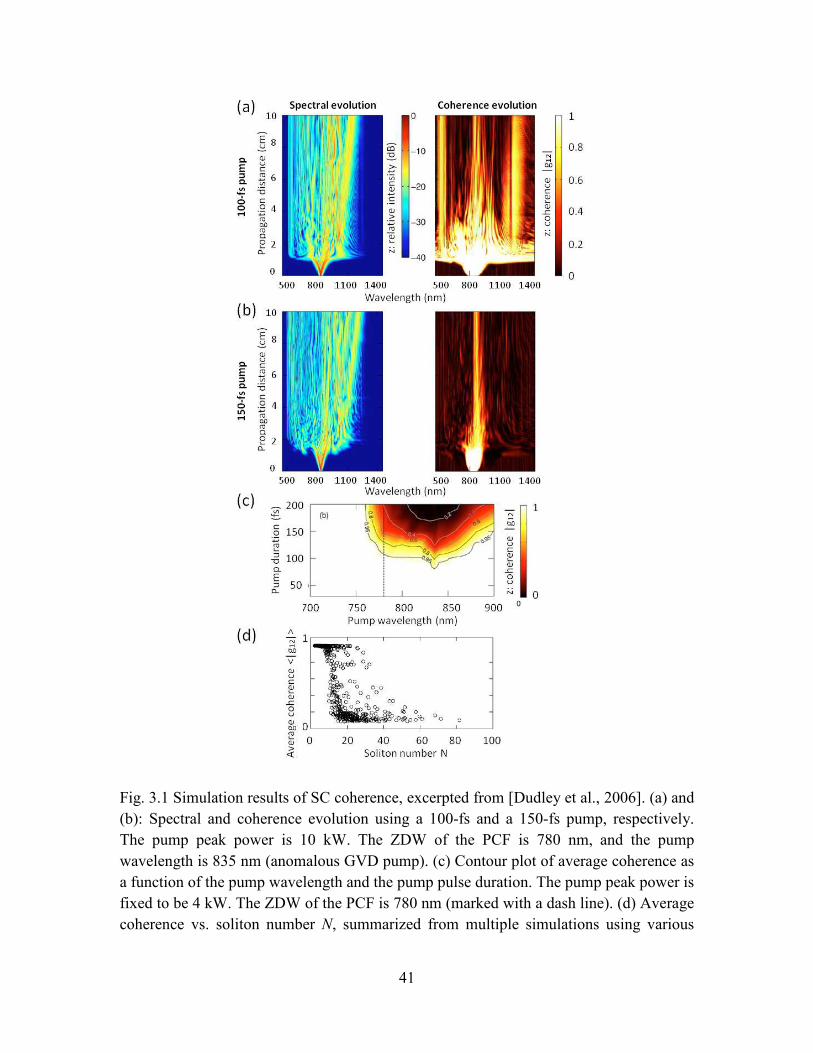
41
Fig. 3.1 Simulation results of SC coherence, excerpted from [Dudley et al., 2006]. (a) and
(b): Spectral and coherence evolution using a 100-fs and a 150-fs pump, respectively.
The pump peak power is 10 kW. The ZDW of the PCF is 780 nm, and the pump
wavelength is 835 nm (anomalous GVD pump). (c) Contour plot of average coherence as
a function of the pump wavelength and the pump pulse duration. The pump peak power is
fixed to be 4 kW. The ZDW of the PCF is 780 nm (marked with a dash line). (d) Average
coherence vs. soliton number N, summarized from multiple simulations using various

42
parameter sets, in which the pump wavelength is ranged 790–900 nm, pump pulse
duration is 30–200 nm, and pump peak power is 3–30 kW.
The following dynamics were found from the results. (1) Shorter pump pulse duration
produces higher coherence. This can be seen by comparing Fig. 3.1 (a) and (b). At a
propagation distance L >> Lfiss, 50-fs pump yields SC of nearly perfect coherence using
the parameter set they used (Fig. 3.1 (a)).
(2) Soliton fission can cause dramatic coherence degradation, as in Fig. 3.1 (b).
(3) Pumping in the normal GVD regime generates SC of nearly perfect coherence.
Moving the pump wavelength into the anomalous GVD regime yields coherence
degradation; however, moving the pump wavelength further into the anomalous GVD
regime restores the coherence. This can be seen in Fig. 3.1 (c).
These dynamics can be explained by a unified story. SPM is a coherence-maintaining
process; while MI can amplify noise. In the normal GVD regime, MI is prohibited, and
coherence is high. In the anomalous GVD regime, if MI is significant before the
broadening spectrum covers the MI gain spectrum, MI amplifies the noise background,
causing coherence degradation. If MI is significant after the pulse has broadened to cover
the MI gain spectrum, MI amplifies coherent radiation, yielding coherent output. Because
dramatic spectral broadening is associated with soliton fission, the criterion of coherence
is based on comparing the characteristic length of MI (LMI) with the characteristic length
of soliton fission (Lfiss). Coherence is high when LMI >> Lfiss, or equivalently the soliton
number
N << 16 (3.1.1),

43
considering Lfiss ~ LD /N and LMI ~ 16LNL. Soliton number thus is a criterion of coherence.
Average coherence vs. soliton number is plotted in Fig. 3.1. (d) by compiling results
using various parameter sets. Each parameter set includes pump wavelength, pump pulse
duration, and pump peak power.
Gu et al. (2003) simulated SC coherence to match with experiment. It was found that
adding quantum noise alone causes almost no coherence degradation (because the short
pump pulses used here TFWHM = 60 fs). Adding 2% pump power fluctuation yields the
same average coherence degradation as measured.
Türke et al. (2007) reported simulations of SC coherence using varying pump pulse
duration T0 and pump peak power P0, and compared them with experimental results. A
fixed propagation length L >> Lfiss and a pump in the anomalous GVD regime were used.
The experimental and the simulated results are similar to that in [Dudley and Coen,
2000a and 2000b; Dudley et al., 2006], if we replace the propagation distance L in Fig.
3.1 (a) and (b) with the pump power. With a 148-fs pump, the coherence remains high
when the SC almost reaches its maximum span; after that, coherence degradation occurs.
With a 410-fs pump, the coherence degrades as soon as the spectrum is relatively broad.
This paper [Türke et al., 2007] discussed the coherence of Cherenkov radiation, and
argued that the coherence degradation of Cherenkov radiation is due to XPM with
solitons. Specifically, although each Cherenkov peak is induced by one corresponding
soliton, any Cherenkov peak interacts with the sum of all solitons through XPM. The
parameters of the solitons vary pulse-to-pulse depending on noise, causing phase
fluctuation in the Cherenkov radiation. Larger soliton number is associated with more

44
interference effect when adding solitons up. This explains why larger soliton numbers are
associated with larger coherence degradation.
The authors also explained why coherence degradation of Cherenkov radiation should not
be explained by Dudley’s MI theory. In the 410-fs pump case in this paper (Fig. 3.2 (c)),
the MI-induced sidebands are weak when soliton fission happens. The ejected solitons
are coherent, but the corresponding Cherenkov radiation is incoherent. This needs to be
explained by the XPM theory above.
Fig. 3.2 Simulated SC and its coherence, excerpted from [Türke et al., 2007]. A 410-fs
pump at 775 nm was used, and the pump peak powers are (a) 0.09 kW, (b) 0.9 kW, and
(c) 5.9 kW. The fiber length is 9 cm. The authors argued that in the case of (c), the MI-
induced sidebands are weak when soliton fission happens, and the ejected solitons are
coherent.
I argue that this explanation needs more evidence. The solitons (radiation at the longer-
wavelength side of the pump) in Fig. 3.2 (c) and even (b) appear to be incoherent. Also,
the fact that MI-induced sidebands are weak does not guarantee that the soliton fission is
coherent. There has not been investigation about how large MI-induced sidebands need to
be in order to cause incoherent soliton fission, as far as I know.
Kobtsev et al. (2005) performed simulations to explain perfect soliton coherence and low
non-solitonic coherence measured in their experiment. They argued low coherence is due

45
to fast spectral oscillations in the non-solitonic region. The simulations showed
oscillation of periods Δω ~ 0.5–1 THz in the non-solitonic region of spectra, caused by
interference between components of close frequencies in the SC. Fluctuation in the pump
power causes these fine structures to shift, and the interference visibility/contrast is
reduced when successive pulses have different intensities at a certain frequency. Note this
intensity inequality cannot be factored out in the data processing (see Eq. 2.4.14),
because the fast-changing fine structures are undetectable in the experiment, due to
averaging.
[Dudley et al., 2006] [Türke, et al., 2007] [Kobtsev et al., 2005]
Noise added - Shot noise
- Raman noise - Shot noise
- Pump power fluctuation - Shot noise
- Pump power fluctuation
Results
(1) Shorter pump duration yields higher coherence.
(2) Coherence degradation is associated with soliton
fission.
(3) Coherence is restored when pump wavelength
moves deep into anomalous GVD regime.
Solitons are coherent, and Cherenkov radiation has
low coherence. (Their data did not
explicitly demonstrate this.)
Solitons have perfect coherence, while non-
solitonic region has low coherence
Theory
Coherence depends on whether MI is significant
before soliton fission. A larger soliton number is
associated with greater degradation of coherence.
Cherenkov radiation has coherence degradation
because it interacts with the sum of all solitons through
XPM.
Fine spectral structures cause coherence
degradation in non-solitonic region.
Table 3.1. Summation of previous simulation research and their theories.
A summation of the simulation research and the theories is listed in Table 3.1.
Besides these papers, many experiment-based papers performed simulations to match and
to interpret experimental results, as introduced in the following section. Most of them
used theories similar to Dudley’s.

46
3.2 Experimental Research of SC Coherence
Experimental research using various parameter sets exists in the literature. Most authors
used the Young’s or the Michelson interferometry set up (see Fig. 2.4). A brief summary
is in Table 3.2.
paper [Gu et al.,
2003] [Lu and
Knox, 2004] [Kobtsev et al., 2005]
[Zeylikovich et al., 2005]
[Nicholson and Yan, 2004]
[Türke, et al., 2007]
λ0 (nm) 800 780, 820, 860, 920
835, 795 1560 780 1550 800
TFWHM (fs) 60 100 50 120 90 2000 188 148 410
P0 (kW) 14.7 12.3 52.8 0.5 0.062 0.025 0.093,
4.7
0.8, 2.5, 5.9, 7.6,
13
0.3, 0.9, 2.1, 2.7,
5.5
frep (MHz) 90 80 100 48 48 50 50 80 80
Pave (mW) 90 112 300 3.3 0.3 2.8 1, 50
11, 34, 80, 102,
175
11, 34, 78, 101,
205
Epulse (nJ) 1 1.4 3 0.068 0.0063 0.056 0.02,
1
0.14, 0.42, 1.0, 1.3,
2.2
0.14, 0.42, 1.0, 1.3,
2.6
ZDW (nm)
770 820 < 795 Two ZDWs:
740, 1700
(anoma-lous
pump) - 730
Lfiber 18 cm 6 cm
tapered fiber 30 cm 1.5 m 1km
6 m hybrid
30 cm tapered fiber
Average |g| 0.56 High, lower,
0.15, 0.7, Respectively
1 at solitons 0.98
High |g| only
around λpump
~0.1 ~0.9
Changes from high
to low when power
increases
becomes lower at lower
powers
Conclusion
Simulations showed
fluctuation in pump power
is major source of
noise
Coherence recovery
when moving pump
wavelength deep into
anomalous GVD
Perfect coherence at
solitons’ central
wavelengths. (small soliton number N~3)
Similar to [Lu and Knox, 2004], with
pumps of low peak powers
Short pump pulses yield
high coherence.
Similar to [Nicholson and Yan, 2004].
Cherenkov radiation has low coherence.
Table 3.2. Key facts of previous experimental research on SC coherence.
Bellini and Hansch (2000) measured the coherence between two independent SC
generated at two separate points in a bulk material, using the Young’s scheme. With a

47
grating, distinct fringes at all wavelengths were obtained (Fig. 2.4 (b)), qualitatively
demonstrating the coherence of SC.
Gu et al. (2003) measured coherence of SC in a PCF for the first time, and performed
simulations to show the main cause of coherence degradation is the pulse-to-pulse
fluctuation of the pump power. In the experiment, replica pump pulses were used to
generate SC in two identical PCFs. Interference was performed in the Young’s scheme.
Spectrally-resolved fringes were recorded (Fig. 2.4 (b)), and 12( , 0)g λ τ was calculated.
Using a pump of 60-fs duration, the average coherence was 0.56. Numerical simulations
were performed to match the experimental results. Adding quantum noise resulted in
almost perfect coherence; further adding 2% fluctuation of pump power reproduced the
average coherence in experiment. This showed that coherence degradation is mainly
caused by the fluctuation of the pump power.
It is a limitation that the two-fiber scheme in [Gu et al., 2003] cannot guarantee identical
1( )E λ% and 2 ( )E λ% up to a normalization constant. In the two-fiber scheme, a beam splitter
was used to split the pump, and the replica beams are coupled into two PCFs that were
carefully made identical. But a beam splitter usually cannot make an exact 50/50 split.
Specifically in [Gu et al., 2003], there was a large difference in the power coupled into
each PCF: 0.25 and 0.58 nJ. Also it is hard to ensure the same coupling efficiency in two
PCFs, the same fiber orientation of the two PCFs, etc. As a result, the independently
generated SC 1( )E λ% and 2 ( )E λ% have quite different spectra, making the discussion of
coherence complicated. For example in Fig. 4, radiation at 930 nm is a soliton in 1( )E λ%

48
but is not a soliton in 2 ( )E λ% , thus the physical meaning of |g12(λ=930 nm)| is complicated.
I think the difference between 1( )E λ% and 2 ( )E λ% might be responsible for part of the
coherence degradation.
Lu and Knox (2004) showed the coherence recovery caused by moving the pump
wavelength deep into the anomalous GVD regime. This result was later reproduced by
simulations [Dudley et al., 2006]. In this experiment, a one-fiber scheme was used for SC
generation. The pump was sent into a fiber for SC generation. Successive SC pulses
1( )E λ% and 2 ( )E λ% interfere in a Michelson interferometer, and the signal was measured
with an OSA. This scheme ensures that 1( )E λ% and 2 ( )E λ% are SC generated under exactly
the same condition, except for different noise seeds. The unequal beam splitting in the
interferometer only yields different normalization constants on 1( )E λ% and 2 ( )E λ% , which
can be factored out in the data processing. Most of later experiments used this
configuration to measure SC coherence.
Zeylikovich et al. (2005) showed similar results to [Lu and Knox, 2004], using a different
parameter set.
Kobtsev et al. (2005) measured the coherence at the central wavelengths of solitons and
at second harmonic wavelengths of the solitons. Using a 50-fs pump, the soliton number
is small N ~ 3. Nearly perfect coherence was measured at the central wavelengths of the
solitons, which is as expected according to Eq. 3.1.1. The second harmonic wavelengths
of the solitons are in the non-solitonic region. Considerable coherence degradation was
shown at these wavelengths. The paper explained that this is due to the fast spectral

49
oscillation in the non-solitonic region, as introduced in Section 3.1. Simulations showed
pump power fluctuation of ~0.5% was enough to reproduce the experimental coherence
degradation in the non-solitonic region.
[Nicholson and Yan, 2004] and [Nicholson et al., 2008] investigated the coherence of all-
fiber-based SC using doped fibers. The 2004 paper showed that SC generated by a fs
pump has much higher coherence than SC by a ps pump. Fibers of different dispersion
properties were spliced together for dispersion management. A piece of SMF of a proper
length was used to compress the pump pulse before it is coupled into the fiber for SC
generation. The 2008 paper investigated optimization of the pulse compression to
generate high-coherence SC.
Türke et al. (2007) measured the coherence of SC using two different pump pulse
durations and selected pump powers. The shorter-duration pump produced higher
coherence than the longer-duration pump, similar to [Nicholson and Yan, 2004].
A summary of the above experimental research is in Table 3.2. I think there are some
limitations of these experiments. (1) The tuning of parameters is limited, due to practical
difficulties. No gradually-changing evolution of the coherence was measured to compare
with simulated evolution such as Fig. 3.1. (a) and (b). (2) No previous experiments
investigated the effect of using different fiber lengths, especially short fibers approaching
the soliton fission length.

50
3.3 My Research
My research focuses on the undone things mentioned in the last paragraph.
(1) Tune the SC power continuously to obtain evolution of spectra and of coherence. It is
expected that the evolution visualize coherence dynamics and allow detailed comparisons
with simulations. Detailed discussions about the coherence mechanisms are thus possible.
(2) Investigate the coherence properties depending on the fiber length, with especial
attention on short PCFs of Lfiber ~ Lfiss. Simulations have shown that coherence
degradation is associated with soliton fission. Using fiber lengths close to the soliton
fission length is expected to clearly show the coherence degradation process, and to show
what fiber length can yield SC of high coherence.

51
4. METHODS
SUMMARY
4.1 describes the experimental procedure. Based on the setups in previous
research, some improvement is made by using the Mach-Zehnder interferometer
and using wedge beam splitters (Fig. 4.3).
4.2 describes the methods of numerical simulation. Section 4.2.2 and 4.2.3
introduce how to obtain the dispersion term and the Raman term, respectively. A
summary of all parameters for simulation is listed in Section 4.2.4. Section 4.2.5
introduces how to model noise and calculate coherence.

52
4.1 Experiment
The PCFs in my experiment are: highly nonlinear SF6 PCFs of different lengths: 10.5
cm, 4.7 mm, 3.9 mm, and 1.0 mm, and a highly nonlinear Tellurite PCF of 2.7 cm.
Fig. 4.1. SEM picture of the cross section of the SF6 PCF. Inset is a close-up of the core.
The core diameter is 3.6 µm.
Fig. 4.2. Microstructure and the dispersion of the Tellurite PCF. (a) Cross section of the
fiber under an optical microscope. (b) and (c) are closeups of the core under SEM and
under an optical microscope, respectively. (d) is the dispersion curve. The ZDW is 1380
nm. These figures are excerpted from [Domachuk et al., 2008].
Key information about these PCFs is compiled in Table 4.1, in comparison with two
silica PCFs and another SF6 PCF. The microstructures and the dispersion curve are
shown in Fig. 4.1 and 4.2. How to calculate the dispersion curve of the SF6 PCF is

53
introduced in Section 4.2.2. The tellurite PCF was previously reported in [Kumar et al.,
2003; Domachuk et al., 2008], where the dispersion curve was reported.
Silica PCF SF6 PCF SF6 PCF Tellurite PCF Equations
Reported in
[Dudley et al., 2006;
Ranka et al., 2000]
[Kumar et al., 2002;
Omenetto et al., 2006;
Moeser et al., 2007]
N.A.
[Kumar et al., 2003;
Domachuk et al., 2008]
dcore (µm) 1.6
(1.7 [Ranka]) 2.6 3.6 2.5
n2 (∙10−20 m2/W)
3 22 22 25
γ ( /km∙W) 110 167.97 87.6 596
2
0
2
eff
n
A
πγλ
=
Aeff = core area of fiber
ZDW (nm) 780
(767 [Ranka]) 1300 ~1300 1380
β2 (ps2 / km)
−11.83 −73.9248 −48.39 −92.19
β3 (ps3 / km)
0.081 0.2434 0.305 0.6411
λ0 (nm) 835
(790 [Ranka]) 1550
Pave (mW) 70 50 P0 (kW) 7 5
TFWHM (fs) 110 T0 = TFWHM
/1.763
LNL (mm) 1.3 0.85 1.6 0.34 01NL
L Pγ=
LD (mm) 329 52.7 80.4 42.2 2
0 2DL T β=
N 15.9 7.9 7.02 11.2 D NLN L L=
Lfiss (mm) 20.7 6.7 11.5 3.8
fiss D
D NL
L L N
L L
=
=
Lfiber (mm) 5.7 17
1 3.9 4.7 105
27
Lfiber/Lfiss 0.85 2.5
0.087 0.34 0.41 9.1
7.1
Table 4.1. Parameters of the PCFs and the pump used in the experiment, in comparison
with a silica PCF and a SF6 PCF in literature. In the column of the silica PCF, the
parameters are for the fiber used in [Dudley et al., 2006] if not otherwise noted.

54
Note these parameters may need correction when matching simulations to experimental
results.
Fig. 4.3. Experimental setup for the measurement of SC coherence.
I used the delayed-pulse method to perform interference between successive SC pulses
generated in one PCF, and measured the spectral fringes using an OSA. The setup (Fig.
4.3) is similar to that in [Lu and Knox, 2004]. An OPO pumped by a mode-locked
Ti:sapphire laser generates laser pulses at λ0 = 1550 nm, of duration TFWHM = 110 fs, at a
repetition rate frep = 80 MHz, and with an average power of 250 mW. λ0 = 1550 nm is in
the anomalous GVD regimes of the SF6 PCF and the tellurite PCF used in the
experiment.

55
A combination of a half wave plate and a polarizer was used to continuously tune the
laser power sent into the PCF. Another half wave plate was used to tune the polarization
of the pump. A 60X aspherical lens was used to couple the laser into the PCF. And
another 60X aspherical lens was used for collimation. The power efficiency of SC
generation is ~30% for all fibers, when coupling loss and collimation loss are included.
The fibers were hand cleaved. In a usual hand cleave, one presses the fiber onto the blade
with a finger, scratches the fiber gently with a scriber, and bends the blade to break the
fiber. It becomes challenging to cleave sub-cm fibers because fingers easily touch and
might damage the facets. I used narrow strips of tape to “press” the fiber onto the blade,
and scratched the fiber carefully while monitoring it under microscope. The tape also
helped to handle the fiber. I was able to cleave fibers as short as ~1 mm.
Sub-cm PCFs were mounted on customized stages of proper sizes; longer PCFs were
mounted on commercial fiber clamps. Using tape to mount the sub-cm fiber onto the
stage is usually better than using glue (Fig. 4.4). Glue usually dries fast and
uncontrollably, while using tape allows fine adjustment of the position and especially the
orientation of the fiber.
Fig. 4.4. 1-mm SF6 PCF mounted on a customized stage using tape.

56
A Mach–Zehnder interferometer with a one-pulse delay (z = c/ frep ~ 3.75 m, with frep =
80 MHz) was built. By using wedge beam splitters, instead of plate, cube, or pellicle
beam splitters, ghosting was mitigated. The Mach–Zehnder design balances the
dispersion in two arms - each beam penetrates the splitter once. The interferometer output
was measured with an OSA (Yokogawa AQ6370B) with a range of 600–1700 nm.
The interference signal 12( )I ω shows fringes with a contrast/visibility as in Eq. 2.4.14.
1( )I ω and 2( )I ω were measured by blocking one of the two arms. Note 12( )I ω , 1( )I ω , and
2( )I ω here are radiation at the detector, which was denoted with “Q” in Chapter 2. In the
data processing, I identified peaks and valleys of the fringes, and calculated the fringe
visibility/contrast, and then calculated 12( )g ω according to Eq. 2.4.14.
The power-dependent coherence evolution 12 ( , )g Pω and spectral evolution 1( , )I Pω and
2( , )I Pω were obtained by repeating the above steps with varying power coupled into the
fiber. Note P is the average power of SC output. The short-arm spectrum evolution
1( , )I Pω is used to represent the SC spectrum, because it has less divergence and higher
intensity than the long-arm one. The spectrally averaged coherence
(1)12 1(1)
12
1
( , ) ( )( )
( )
g P Ig P
I
ω ωω
⋅=∑
∑ (4.1.1)
was calculated to represent the overall coherence.

57
4.2 Simulation
4.2.1 Introduction
SC generation is modeled using the frequency-domain GNLSE with approximation (Eq.
2.2.64). It can be directly solved using ordinary differential equation (ODE) solvers.
“ODE45” solver in MATLAB is used here. The solver automatically finds optimal step
lengths to satisfy user-specified precisions. The code provided in [Dudley and Taylor,
2010] is used, with some adjustment. This code does not include noise. How to model
noise and calculate coherence is introduced in Section 4.2.5.
The pump is sech2 pulses with an optional linear chirp:
2
0 20 0
( 0, ) sech exp2
t C tA z t P i
T T
= = −
(4.2.1),
in which P0 is the peak power of the pulses, T0 = TFWHM /1.763, and C represents a linear
chirp. The frequency-domain representation is
( 0, ) ( 0, )A z FT A z tω= = =% (4.2.2).
This is the initial state of the GNLSE. Noise should be added when needed.
Specific dispersion and Raman terms in the GNLSE can either be found in literature or be
calculated as follows.

58
4.2.2 The dispersion term
The theory about the dispersion term is introduced in Section 2.2.2.
The dispersion curve of the SF6 PCF used in my experiment cannot be found in
literature. It is thus estimated based on the dispersion curves of some other SF6 PCFs in
[Kumar et al., 2002], and later corrected by comparing simulated SC spectra to
experimental ones. The dispersion curve of the tellurite PCF used in my experiment was
reported in [Kumar et al., 2003; and Domachuk et al., 2008] (Fig. 4.2 (b)).
To convert GVD β2(ω) to the dispersion term B(ω) in the GNLSE, two methods were
introduced in Section 2.2.2. Method (1) is used here, which is to calculate the expansion
coefficients βk based on β2(ω), and then calculate B(ω). In this way the result B(ω) can be
extended to any interested bandwidth. Using method (2) yields results only for the
bandwidth that the original GVD curve covers.
Specifically, GVD reported in those papers are in terms of D(λ), which is another
representation of GVD other than β2(ω). The numerical data of D(λ) were extracted from
the figure in the paper using an unofficial Matlab application “grabit” [Doke, 2007].
Using ω = 2πc/λ and
22
2( ) ( )
cD
πω β ωλ
= − (2.2.37),
D(λ) can be converted to β2(ω). Then considering
22 2 0 0 3 0 0 4 0
1( ) ( ) ( ) ( ) ( ) ( ) ...2!β ω β ω ω ω β ω ω ω β ω= + − + − + (2.2.39),

59
curve fitting is performed to obtain β2 and β3, and also higher-order dispersion if
necessary.
Fig. 4.5. Calculation of the dispersion of the SF6 PCF. (a) Calculating the dispersion
curve of the 3.6-μm-core PCF based on the dispersion curves of a 2.6-μm and a 4-μm-
core SF6 PCFs, through linear interpolation. The 2.6-μm and the 4-μm-core curves are
excerpted from [Kumar et al., 2002]. (b) Linear curve fitting of β2(ω−ω0)|3.6-μm.
Model linear
y = p1*x + p2 quadratic
y = p1*x^2 + p2*x + p3 p1 0.305 0.0001266 p2 -48.39 0.2784 p3 -47.66
SSE 37.24 8.949 R-square 0.999 0.9998
Table 4.2. Polynomial fitting of the β2(ω−ω0) curve for the 3.6-μm-core SF6 PCF.
Fig. 4.5 shows the process to calculate β2 and β3 of the SF6 PCF. Fig. 4.5 (a) shows the
D(λ) curve of the 2.6-μm-core and the 4-μm-core SF6 PCF reported in [Kumar et al.,
2002], and D(λ) curve of the 3.6-μm-core SF6 PCF calculated based on linear
interpolation. Fig. 4.5 (b) shows the β2(ω−ω0) curve converted from the D(λ) curve. A
linear curve fitting is chosen to reproduce the β2(ω−ω0) curve, yielding β2 = −48.39
ps2/km and β3 = 0.305 ps3/km. The details of the curve fitting are in Table 4.2. Note the
fibers of 2.6-µm-core and 4-μm-core in [Kumar et al., 2002] are SF6 PCFs of a different

60
micro pattern than the ones used in my experiment, so the validity of this calculated
dispersion curve needs to be carefully tested by comparing simulations with experimental
measurement. In fact, major modifications of the dispersion were made to match with
experimental data (Section 5.1.2).
For the tellurite PCF, the D(λ) curve (Fig. 4.2 (b)) was reported in [Domachuk et al.,
2008]. Using the same method, the results of curve fitting were obtained as in Table 4.3.
In this case, the quadratic fitting is chosen, yielding β2 = −92.19 ps2/km, β3 = 0.6411
ps3/km, and β4 = −0.59*10-3 ps4/km (β4 = 2*p1). This fitting curve was later found to be
inaccurate for wavelengths longer than about 2 μm. Major modifications were made to
match with experimental data (see Section 5.2.2).
Model Linear
y = p1*x + p2 quadratic
y = p1*x^2 + p2*x + p3
cube y= p1*x^3 + p2*x^2 +
p3*x + p4 p1 0.4576 -0.000295 5.709e-07 p2 -75.07 0.6411 -0.0008276 p3 -92.19 0.767 p4 -97
SSE 1.136e+05 1.191e+04 547.8 R-square 0.9858 0.9985 0.9999
Table 4.3. Polynomial fitting of the β2(ω−ω0) curve for the tellurite PCF.
4.2.3 The Raman term
The theory about calculating the Raman function was introduced in Section 2.2.3.
The Raman response function of SF6 has been reported [Heiman et al., 1979; Aber et al.,
2000; Kalashnikov et al., 2007; and Moeser et al., 2007]. Here the model in [Kalashnikov

61
et al., 2007] is used, where the Raman response function is modeled as Eq. 2.2.61, with
1τ = 5.5 fs, 2τ = 32 fs, and Rf = 0.13 (Fig. 4.6).
Fig. 4.6. Raman response function hR(t) of SF6. It is modeled as Eq. 2.2.61, with 1τ = 5.5
fs, 2τ = 32 fs, and fR = 0.13.
The composition of my tellurite fiber is 75TeO2–12ZnO–5PbO–3PbF2–5Nb2O5. The
Raman gain spectra of a few similar compositions have been reported. 77.1TeO2–
22.9ZnO was measured in [Plotnichenko et al., 2005], and the result is denoted here as
Raman gain spectrum 1, 1Rg . Stegeman et al. (2006) used TeO2–TiO0.5–PbO, and Qin et
al. (2007) used TeO2–Bi2O3–ZnO–Na2O, showing similar results of Raman gain spectra
(denoted here as Raman gain spectrum 2, 2Rg ). 1R
g and 2Rg have similar shapes, but
different magnitudes. 1Rg is ~2.3× higher than 2R
g , according to the ~735-cm-1 peak. As a
result, 1Rg yields an invalid R
f = 1.37. 2Rg is used here, yielding fR= 0.55 and hR(t) as in
Fig.4.7 (b). A comparison of these two cases is in Table 4.4.

62
Fig. 4.7. (a) Raman gain spectra gR(ω) of tellurite glasses. The green curve gR1 was
reported in [Plotnichenko et al., 2005], and the blue curve gR2 was reported in [Stegeman
et al., 2006; Qin et al., 2007; Yan et al., 2010]. Both are calibrated for pump wavelength
λ0 = 514.5 nm. (b) Raman response function hR(t) calculated based on gR2, using Eq.
2.2.57.
gR1 gR2
Reported [Plotnichenko et al., 2005] [Stegeman et al., 2006; Qin et
al., 2007; Yan et al., 2010]
Composition 77.1TeO2–22.9ZnO
(material 1) TeO2–Bi2O3–ZnO–Na2O [Qin]
(material 2)
Pump 0λ (nm) 514.5
632.8 (converted to 514.5 using
01R
g λ∝ )
Major peak frequency (cm-1) ~430, ~660, ~735
( 1Rg and 2R
g have similar shapes)
733-cm-1 peak value (10^-13 m/W)
109 (= 57*peak value
of 2[SiO ]R
g )
38.5 (Converted to 47.2, which is 25*peak value of 2[SiO ]
Rg )
( )R
h t Similar
Rf 1.37 0.55
Table 4.4. Comparison of two Raman gain spectra: gR1 reported in [Plotnichenko et al.,
2005] and gR2 reported in [Stegeman et al., 2006; Qin et al., 2007; Yan et al., 2010], and
calculation of the Raman term.

63
4.2.4 Simulation parameters
The parameter values for simulation are listed in Table 4.5. Note they might need to be
optimized in order to match simulations to experimental measurement (see Ch. 5).
Parameter SF6 PCF Tellurite PCF
Pump wavelength 0λ (nm) 1550
Pump pulse durationFWHM
T (fs) 110
Pump chirp 0
Pump power fluctuation (%) 2
Fiber length fiberL (mm) 105, 4.7, 3.9, 1 27
Loss (dB/m) 4
Dispersion 2β = −48.39 ps2/km,
3β = 0.305 ps3/km
2β = −92.19 ps2/km,
3β = 0.6411 ps3/km,
4β = −0.59*10-3 ps4/km
Nonlinearity γ (/km∙W) 87.6 596
Raman fractionR
f 0.13 0.55
Raman response function ( )R
h t 1τ = 5.5 fs, 2τ = 32 fs
(Eq. 2.2.61)
Numerical curve as in Fig.4.7
(b)
Table 4.5. Values of parameters for simulation (subject to change in the optimization
process).
The nonlinearity γ can be calculated based on the assumption that the effective mode area
is just the area of the fiber core:
0 2 2 22 2
0 0
82
4eff core core
n n n
cA d d
ω πγλ π λ
= = = (4.2.3).
For our SF6 PCF, γ = (8*22*10−20 m2/W)/(1.55*10−6 m * (3.6*10−6 m)2) = 0.0876 /m·W
= 87.6 /km·W.
For our tellurite PCF, dcore = 2.5 µm was reported [Domachuk et al, 2008], so core area
should be π·dcore2/4 = 4.9 µm2. But an effective mode area of 1.7 µm2 was reported

64
[Domachuk et al, 2008]. Using this value, γ = (2π*25*10−20 m2/W)/(1.55*10−6 m *
1.7*10−12 m2) = 0.596 /m·W = 596 /km·W.
4.2.5 Modeling noise and coherence
In the experiment, spectral interference fringes were measured, and then coherence was
calculated using
[ ]1 2
1 2m min12
m min 1 2
2 ( ) ( )( )( ) ( )
( ) ( ) ( )ax
ax
I II IV g
I I I I
ω ωω ω
ω ω−= =+ +
(2.4.14).
In the simulations, coherence was calculated directly using its definition:
*1 2
12
1 2
( ) ( )( )
( ) ( )
E Eg
I I
ω ωω
ω ω=
% %
(2.4.12).
Considering
0 0 0 0( , ) ( , , ) ( , )exp( )E r F x y A z i zω ω ω ω ω ω β− = − −r %% (2.2.3),
the modal distribution F can be ignored, and there is
*1 2
12
1 2
( ) ( )( )
( ) ( )
A Ag
I I
ω ωω
ω ω=
% %
(4.2.4).
Simulations using the GNLSE were repeated for N (here 20) times with independent
noise to generate SC fields ( )mA ω% , m = 1, 2, …, N. The noise includes: (a) quantum-limit
shot noise in the pump, and (b) pulse-to-pulse fluctuation of the pump power.

65
Spontaneous Raman noise was not included here, because it has been found to cause
coherence degradation two orders of magnitude smaller than shot noise does [Corwin et
al., 2003; Dudley et al., 2006].
Specifically, the shot noise is one photon of a random phase in each frequency grid:
( ) ( ) expnoise noise RA A iω ω φ=% (4.2.5).
The random phase Rφ obeys a uniform distribution between 0 and 2π:
(0,2 )R
Uφ π∈ (4.2.6),
where ( , )U a b is the uniform distribution between a and b.
Considering the energy of the photon
2
( )noiseE A dfω ω= =h (4.2.7),
there is
( )noiseA dfω ω= h (4.2.8),
in which the frequency f = ω/2π, and df is the increment of the frequency grid.
The pulse-to-pulse fluctuation of the pump power obeys a normal distribution with a
certain standard deviation x% (e.g., x = 2). The peak power of a pulse is
0 0 PP P= ⋅∆ (4.2.9),

66
in which
( 1, %)P
N xµ σ∆ ∈ = = (4.2.10).
( , )N µ σ is the normal distribution with a mean μ and a standard deviation σ.
0P is the average peak power of pump pulses:
0
0.88
rep FWHM
PP
f T= (4.2.11),
in which P is the average power of the laser, repf is the repetition rate, and FWHMT is the
duration of the pulse.
Eq. 4.2.4 was calculated as follows. The ensemble average is the average of all non-
identical pairs: m n≠ , m, n = 1, 2, …, N. Writing the explicit form of in Eq. 4.2.4
yields
*
12 1 22 2
( ) ( )( )
( ) ( )
m nm n
m nm n
A Ag
A A
ω ωω
ω ω
≠=
% %
% %
[ ]*
2
( ) ( ) ( 1)
( )
m n
m n
m
m
A A N N
A N
ω ω
ω≠
−=∑
∑
% %
% (4.2.12).
In the denominator,

67
2
1 2( ) ( ) ( )m
m
I I A Nω ω ω= =∑ % (4.2.13),
because m and n are from the same pool: m, n = 1, 2, …, N. I1(ω) and I2(ω) are average
spectra of the short/long arm, respectively.
Eq. 4.2.12 and 4.2.13 are consistent with the practical experiment, where the photo
detectors are slow. There is usually different attenuation in two arms of the
interferometer. This intensity imbalance was factored out in the data processing (Eq.
2.4.14), so it does not need to be included here.
Suppose a fast detector is used and it can distinguish each pulse, and the single-shot
coherence is
[ ]
* **1 2
12 single-shot 1 2 1 22 21 2
( ) ( ) ( ) ( )( ) ( )( )
( ) ( )( ) ( ) ( ) ( )
m n m n
m nm n
A A A AA Ag
A AI I A A
ω ω ω ωω ωωω ωω ω ω ω
= = =
% % % %% %
% %% %
( ) ( ) exp arg ( ) arg ( )m ni A Aω ω = − − % % (4.2.14),
in which ( )arg means the argument of a complex number: [ ]arg exp( )iφ φ= , 0 ≤ ϕ < 2π.
In this case the averaged coherence (Eq. 4.2.4) becomes something that involves only the
phase:
12_ 12 single-shot( ) ( )PHASE m ng gω ω
≠=
12 single-shot( )
( 1)m n
g
N N
ω≠=
−
∑

68
( ) ( ) exp arg ( ) arg ( )
( 1)
m n
m n
i A A
N N
ω ω≠
− −
=−
∑ % %
(4.2.15).
Its physical meaning is, as mentioned above, a fast detector is used and it can distinguish
each pulse. As a result, the coherence involves only the phase, and not the intensity.
Eq. 4.2.12 is the practical experimental case where the intensity fluctuation in the
spectrum and the phase correlation both contribute to the coherence. Eq. 4.2.15 involves
only the phase. Some coherence degradation has been thought to be related to the
intensity fluctuation of the SC spectrum, so these two definitions are used here to isolate
the effects of the intensity fluctuation and the phase instability.
The pulse-to-pulse stability of spectral intensity is:
( )2( ) ( ) ( ) ( ) ( )v I m m m mC I I I Iω σ ω ω ω ω− = − = − − (4.2.16),
in which Cv is the coefficient of variation, σI is the standard deviation of spectral
intensity, is the mean with respect to all pulses, and2
( ) ( )m mI Aω ω= % . The negative
sign is used such that higher values of –Cv correspond to higher stability. The maximum
value of –Cv is 0, meaning no pulse-to-pulse fluctuation in spectral intensity. Evolution
−Cv(λ,P) and spectrally-averaged curve –Cv(P) were obtained similarly as coherence
evolution and averaged coherence.

69
5. RESULTS AND DISCUSSIONS
SUMMARY
This chapter presents experimental and simulated results followed by analysis
and discussions about the physics of supercontinuum (SC) and its coherence.
5.1 is about SC generated from different lengths of SF6 PCFs. In 5.1.1,
measured spectral and coherence evolution is presented. In 5.1.2 and 5.1.3,
simulation results are presented. Optimization of the simulations to match
experimental measurements is demonstrated, and the physical meaning of the
results is discussed. 5.1.4 concludes this section.
5.2 is about the results using the tellurite PCF. It is organized similarly as 5.1.

70
5.1 Results Using SF6 PCFs
5.1.1 Experimental results
Fig. 5.1. Spectral evolution (a)–(c) and coherence evolution (d)–(f) of SC generated in
three different lengths of SF6 PCFs (10.5-cm, 4.7-mm, and 3.9-mm). The red arrows in
(a) mark soliton trajectories. The green arrow in (b) marks the Cherenkov peak. The
spectral evolution is calibrated such that the maximum intensity is 0 dB. The lower limit
of the color bar is set to −40 dB so that the 40-dB bandwidth is visualized in the

71
evolution; the upper limit is set for optimal visualization of features. (g)–(i) are line plots
of representative spectra.
Fig. 5.1 shows measured spectral and coherence evolution of SC generated in different
lengths (10.5-cm, 4.7-mm, and 3.9-mm) of SF6 PCFs, plotted in contour maps. The y
axes of the contour maps are the average power of SC. Line plots of representative
spectra are also shown (Fig. 5.1 (g)–(i)).
In the 10.5-cm-fiber case, the spectral evolution (Fig. 5.1 (a)) shows a soliton-fission-
dominated pattern. Three solitons are marked with red arrows. Ejection of the first soliton
occurs at ~10 mW, accompanied with the emergence of the Cherenkov peak at ~1070
nm. Solitons show Raman-induced red shift when the power increases. The coherence
(Fig. 5.1 (d)) is high for only the initial stage of broadening, and degrades quickly after
soliton fission.
The SC from the 4.7-mm fiber (Fig. 5.1 (b)) has two symmetric spectral lobes at both
sides of the pump wavelength for power less than ~45 mW, indicating a SPM-dominated
regime. At ~45 mW, strong spectral broadening occurs, indicating strong temporal
compression, and soliton fission is about to happen. Although no soliton trajectory was
captured due to the limited wavelength range of measurements, the Cherenkov peak
(marked with a green arrow) emerging at ~850 nm ~60 mW is the evidence of a
corresponding soliton. The coherence properties (Fig. 5.1 (e)) show association with
soliton fission. High coherence (~0.9) was maintained for power less than ~45 mW
(before soliton fission). For power higher than ~45 mW (after soliton fission), coherence
degradation occurs at most parts of the spectrum.

72
For the 3.9-mm case, the story is less apparent by looking at Fig. 5.1 (c) and (f) alone.
Fig. 5.1 (c) and (f) (0–84 mW) can be associated to the 0–~50 mW part of Fig. 5.1 (b)
and (e), respectively. In Fig. 5.1 (c), the SC reaches ~1000 nm at the power ~75 mW,
similar to the situation when the power is ~50 mW in the 4.7-mm case (Fig. 5.1 (b)). This
indicates strong temporal compression, and soliton fission is just going to happen. At the
same time, coherence degradation starts to occur at wavelengths far from the pump (at P
~75 mW in Fig. 5.1 (f)). If increasing the power above 84 mW, the consequent dynamics
should be similar to what happen at powers greater than ~50 mW in the 4.7-mm case.
Unfortunately, these dynamics were not measured, due to the limited power of the pump.
The fluctuation of coherence at wavelengths below 1400 nm (Fig. 5.1 (f)) will be
discussed later (Section 5.1.3).
SC in the 1.0-mm SF6 PCF shows a pure SPM pattern. It reaches a 40-dB bandwidth of
about 250 nm at the maximum power. Since we are mostly interested in broad SC,
discussion about this SC will be in a separate paper.
The above results show association between coherence degradation and soliton fission.
Using a fiber slightly shorter than the soliton fission length, SC of almost perfect
coherence can be generated with little sacrifice in bandwidth.

73
5.1.2 Simulated spectral evolution and discussions
Fig. 5.2. (a)–(c) Experimentally measured spectral evolution using three different lengths
of SF6 PCF, respectively. (d)–(f) Corresponding simulation results. The vertical black
line at 1700 nm helps visually comparing with the experimental data. (g) and (h):
Simulated spectral and temporal evolution depending on the propagation length. P = 77
mW is used. It is shown graphically that soliton fission happens at ~9 mm. Analytically
calculated soliton fission length is similar Lfiss = 10.2 mm. (i) GVD D(λ) of the fiber. The
red lines mark the zero dispersion wavelength (ZDW) and the pump wavelength (1550
nm). The ZDW is ~1370 nm. The GVD at the pump wavelength is ~38 ps/(nm∙km).
Simulated spectral evolution is plotted in Fig. 5.2, in comparison with the experimental
results. For the short fibers (4.7 and 3.9 mm), the simulations show much “slower”
evolution, which can be quantified by the soliton fission length Lfiss or the power at which

74
soliton fission happens. Specifically, the simulations (Fig. 5.2 (g) and (h)) graphically
show soliton fission at ~9 mm, when P = 77 mW (same as the maximum power in the
4.7-mm-fiber case of the experiment). P is the average power of SC. Analytically
calculated soliton fission length is close: Lfiss = 10.2 mm (using Eq. 2.3.17), when P = 77
mW. In the measurements, soliton fission happens between 3.9 and 4.7 mm, when P = 77
mW.
To fix this mismatch in the soliton fission length, the simulated Lfiss needs to be shortened
by about a half. Considering Lfiss = 20 2 0T Pβ γ (Eq. 2.3.17), in which the duration of
the pump pulses T0 = TFWHM /1.763, |β2| = |β2(ω0)|, and the peak power of the pump pulse
P0 = 0.88∙P/(frep∙TFWHM), there is
320.6fiss FWHM repL T f Pβ γ= (5.1.1).
Tuning down TFWHM and tuning up P, γ, and |β2| in the simulations can help fixing the
mismatch in Lfiss. Tuning the chirp of the pump C is also considered, because it affects the
beginning stage of the evolution and the soliton fission length too.
The simulations can be optimized by iteratively tuning parameters and manually
comparing features with experiments. The parameters can be tuned in 3 steps: (1)
duration of pump pulses TFWHM, (2) the average power of SC P, the nonlinearity of the
fiber γ, and GVD of the fiber |β2|, (3) the chirp of the pump C. Tuning in this order allows
for easier comparison of features.

75
Fig. 5.3. Optimization of the duration of the pump pulse TFWHM. Red curve: measured
output spectrum at P = 2 mW and Lfiber = 3.9 mm. Black curves: simulated output
spectrum using a pump of transform-limited sech2 pulses of TFWHM = 100, 110, and 120
fs, respectively, also at P = 2 mW and Lfiber = 3.9 mm.
The duration of the pump pulse TFWHM was optimized by inspecting the output
bandwidth. TFWHM determines the pump bandwidth, which in turn affects the output
bandwidth. It is ideal to inspect cases of low SC powers and short fibers, because there is
little broadening, other parameters are less involved, and thus the output bandwidth is
highly dependent on TFWHM in these cases. Here the case of P = 2 mW and Lfiber = 3.9 mm
is investigated, and the measured output spectrum is between the simulated output spectra
using transform-limited sech2 pulses of TFWHM = 110 fs and 100 fs as the pump (Fig. 5.3).
So TFWHM was modified from 110 to 105 fs. In fact the simulations show no appreciable
broadening from the pump to the output. Although it is more straightforward to
experimentally measure the pump duration and the chirp, our goal is to determine as
many parameters as possible and avoid experimentally measuring them.

76
Fig. 5.4. Optimization of the simulated spectral evolution. Each line includes four plots of
spectral evolution: the beginning (low power) part of the 10.5-cm-fiber case, the 10.5-
cm-fiber case, the 4.7-mm-fiber case, and the 3.9-mm-fiber case. (a) Experimental data.
(b) Simulations with TFWHM = 105 fs has been applied. (c) Simulations after further tuning
P to 1.3*P and γ to 1.38*γ. (d) Simulations after further tuning β2(ω) to 2*β2(ω).
The product of P∙γ can be considered as one parameter to tune. For any pair of positive
coefficients a and b of a fixed product (a∙b = constant), tuning P to a∙P and γ to b∙γ yields

77
invariant SC spectrum, up to a calibration constant. This can be seen in the GNLSE (Eq.
2.2.30 and 31) by considering2
P A∝ . Tuning up P∙γ enhances SPM, and causes soliton
fission to happen earlier. One major feature of the SPM-based broadening is the spectral
lobes at both sides of the pump wavelength (e.g., see the changes from Fig. 5.4 (b) to (c),
4.7- and 3.9-mm-fiber cases).
Tuning |β2| (=|β2(ω0)|) was implemented by multiplying the whole curve of β2(ω) by a
constant. For example, tuning β2(ω) to a*β2(ω) was applied when tuning |β2| to a*|β2| is
needed; a is a real coefficient. The reason is that tuning |β2| alone will change the shape of
the β2(ω) curve. For example, the ZDW will be changed. Multiplying β2(ω) by a constant
avoids this issue. Simulations show tuning up |β2| has a small impact on the two spectral
lobes at both sides of the pump wavelength, but causes soliton fission to happen earlier
(see e.g., the changes from Fig. 5.4 (c) to (d), 4.7- and 3.9-mm-fiber cases).
The above dynamics of tuning P∙γ and |β2| can be understood physically as follows. SPM
is based on the nonlinear refractive index 0 2n n n I= + . Considering I ∝ P and n2 ∝ γ,
tuning up P or γ similarly enhances SPM. On the other hand, soliton fission happens
when the pulse evolves to the shortest duration, and this timing depends on both SPM and
dispersion. As a result, the soliton fission length depends on P, γ, and |β2|.
Tuning P∙γ to ~1.8*P∙γ optimizes the SPM-based broadening (Fig. 5.4 (c) to (d)).
Assuming tuning P to 1.3*P, which indicates a 23% collimation loss in the experiment, γ
should be tuned to 1.8/1.3*γ = 1.38*γ = 120.9/km∙W. Further tuning β2(ω) to ~2*β2(ω)
yields similar soliton fission lengths as in the experiment (Fig. 5.4 (c) to (d)).

78
The effect of adding a linear chirp C in the pump is illustrated in Fig. 5.5, using the 4.7-
mm-fiber case. SPM induces positive chirps at the central parts of the spectrum. A
positive initial chirp (C > 0) adds up with the SPM-induced chirp, and enhances spectral
broadening. As a result, soliton fission happens earlier. In this case, there is a feature in
the spectral evolution: the flattened central part of the spectrum. A negative initial chirp
(C < 0) has opposite effects, causing soliton fission to happen later. The spectral features
are enhanced oscillation structures, and narrowing or lack of broadening at the beginning
of the spectral evolution. Fig. 5.5 shows the change in the soliton fission power
(represented by the power where the Cherenkov radiation occurs) and in the features,
depending on the initial chirp.
Fig. 5.5. Simulated spectral evolution with varying initial chirps, in the case of the 4.7-
mm SF6 PCF. Adding positive or negative initial chirps causes features in the spectra,
and changes the power at which soliton fission happens. Emergence of the Cherenkov
peak is marked with red lines to represent the powers at which soliton fission happens.

79
Fig. 5.6. Comparison between (a) the measured spectral evolution and (b)–(d)
corresponding simulations using varying initial chirps, for the case of the 3.9-mm SF6
fiber. (a) shows gaps (marked with arrows) between the central peak and the spectral
lobes. (b) and (c) also have these gaps, while in (d) a positive chirp (C = 0.1) flattens the
central parts of the spectrum and causes the gaps to disappear. Spectra at P = 40 mW are
stacked in (e) to show the features clearly.
It is possible to determine the initial chirp C based on the soliton fission power (Fig. 5.5
vs. Fig. 5.2 (b)). It was found that the features mentioned above are more subtle
indicators. The case of the 3.9-mm fiber was investigated for this step, since the
measured data using the 4.7-mm fiber is not ideal in resolution. In the measurements of
the 3.9-mm-fiber case, there are gaps (marked with arrows in Fig. 5.6 (a)) between the
central peak and the spectral lobes at both sides. Simulations with C = −0.1 and 0 have
these gaps, while adding C = 0.1 flattens the central parts of the spectrum and causes the
gaps to disappear. Spectra at P = 40 mW are stacked up in Fig. 5.6 (e) to better show

80
these features. Based on this, it can be decided that the pump has C < 0.1 in the
experiment.
The lower limit of the chirp C can be determined by investigating the broadening at the
beginning (low SC power) part of the evolution. As in Fig. 5.7, the experiments do not
show the lack of broadening as in the simulated case of C = −0.1. So the pump has C >
−0.1 in the experiment.
Fig. 5.7. Comparison of the broadening trends at the beginning (low SC power) part of
the spectral evolution. The case of 3.9-mm SF6 PCF is used. Output spectra at P = 2, 4,
6, 8, 10, 12, 14, 16, 18, and 20 mW are stacked in each plot. The simulations with initial
chirp = −0.2 and −0.1 show narrowing or lack of broadening. This is not seen in the
experiments. So the chirp in the experiment was > −0.1.

81
By now it has been shown that the pump has a small or no chirp (−0.1 < C < 0.1) in the
experiment. C = 0 was chosen as the optimal. The uncertainty in the chirp yields a small
uncertainty in the soliton fission length or power. The examples in Fig. 5.5 show a
change of about 5% in the soliton fission power when tuning C from −0.1 to 0.1.
The above steps (1)–(3) of parameter tuning should be repeated to approach optimal
match. In the above case, repeating step (1) still shows TFWHM should be 105 fs.
Repeating (2) and (3) still yields the same results.
So Fig. 5.4 (d) shows the optimized simulations. Comparisons with the measurements
(compare Fig. 5.4 (d) with (a)) show agreement in the broadening extents, in the soliton
fission powers, and in the emergence of Cherenkov radiation. The analytically calculated
Lfiss is now ~5.4 mm when P = 77 mW, matching the experimental results where Lfiss
should be between 3.9 and 4.7 mm.
There are some mismatches in the wavelengths of solitons (in the 10.5-cm case) and of
the Cherenkov radiation (in the 10.5-cm and the 4.7-mm cases). The soliton wavelength
is determined by the Raman-induced frequency shift 42 0z TβΩ ∝ , in which T0 is the
duration of the soliton. In the 10.5-cm case, the experiments and the simulations show
agreement in the trajectory of the first soliton, but some discrepancies in the trajectories
of the second and the third ones. Tuning the dispersion curve should affect all solitons at
the same time, and thus may not be the cure for these discrepancies. Inaccuracy in the
soliton duration could be responsible for the mismatches, especially considering the
inverse quartic dependence. Cherenkov radiation is phase matched with solitons, so

82
inaccuracy in the soliton wavelengths and in the dispersion should be both responsible for
the mismatches in the wavelengths of the Cherenkov radiation.
The above process demonstrates in principle that, given a spectral evolution, the fiber
length, and the average power of SC, all other parameters can be determined
unambiguously, and the spectral evolution can be reproduced in simulations. Most
importantly, the soliton fission length or power was reproduced quantitatively. Such
optimization allows parameters to be estimated, and avoids experimentally measuring
them.
In future research, a cost function should be developed to quantify the match of features.
Then iterative optimization can be easily implemented by computer. More sophisticated
tuning of parameters, for example tuning the shape of the dispersion curve, can be added
for more subtle optimization.
5.1.3 Simulated coherence and discussions
After the above optimization, the pulse-to-pulse fluctuation of the pump power ΔP is the
only parameter to tune in order to match the simulated and the measured coherence.
Tuning ΔP could not match the coherence in the three fiber lengths at the same time. 5%
fluctuation was chosen for optimal match in the 3.9-mm-fiber case. Simulated coherence
is plotted in Fig. 5.8, in comparison with the experimental results. Fig. 5.8 (a)–(d) are
power-dependent evolution, and (e) and (f) are spectrally-averaged coherence depending
on the power.

83
Fig. 5.8. Simulated coherence of SC generated in three different lengths of SF6 PCFs, in
comparison with the experimental results. Column (a): three plots of measured spectral
evolution using different fiber lengths. Column (b): measured coherence evolution.
Column (c): simulated spectral evolution. Column (d): simulated coherence evolution.
The simulation plots have black lines at 1700 nm to help visual comparison with
experiments. In the experiment, radiation of relative intensity lower than about −40 dB
was not measurable due to the sensitivity limitation; and in the simulations this part of
radiation was also ignored. (e) and (f): spectrally-averaged coherence as functions of the
average SC power. In the simulations, shot noise and 5% pulse-to-pulse power
fluctuation in the pump were added. In (a), the color bars for the 10.5-cm and the 4.7-mm
cases are omitted for clarity, and can be found in Fig. 5.1. In (b)−(d), each color bar
works for three plots in the column.
The simulated and the experimental coherence show qualitative agreement which
confirms the association between coherence degradation and soliton fission. There is

84
some discrepancy, primarily in the extent and rate of degradation. For the short-fiber (4.7
and 3.9 mm) cases, the experiments show quicker degradation at soliton fission than the
simulations. This can be seen in the average coherence (compare Fig. 5.8 (e) with (f) , the
4.7- and 3.9-mm cases), and also in the evolution where the experiments show relatively
abrupt drop of coherence starting at certain powers, whereas the simulations show
coherence degradation starting earlier at the edges of bandwidth and gradually spreading
to larger ranges of wavelength (compare Fig. 5.8 (b) with (d), the 4.7- and 3.9-mm cases).
For the 10.5-cm-fiber case, the average coherence drops to below 0.2 after soliton fission
in the experiments, while to 0.6–0.4 in the simulations (compare Fig. 5.8 (e) with (f), the
10.5-cm cases). In the evolution (compare Fig. 5.8 (b) with (d), the 10.5-cm cases), the
experiments shows surviving coherence at very limited wavelengths after soliton fission,
while in the simulations some coherence is maintained in the non-solitonic region and
along solitons.
The pulse-to-pulse stability of spectral intensity (–Cv, defined in Eq. 4.2.16) and
coherence (|g|) are both figures of merit of SC stability. They might be expected to show
similar trends. –Cv is related to coherence, according to the definition of coherence (Eq.
4.2.12). It has been shown that –Cv has minor contribution in determining coherence
[Dudley et al., 2006]. Here following simulations show that –Cv has low correlation with
coherence, and with the pulse-to-pulse stability of spectral phase (|gPHASE| defined in Eq.
4.2.15).

85
Fig. 5.9. Comparison between pulse-to-pulse stability of spectral intensity (–Cv) and
coherence. (a) Power-dependent evolution of –Cv, using the 4.7-mm SF6 PCF. This can
be compared with the 4.7-mm coherence evolution in Fig. 5.8 (d). (b) The spectral
evolution, (c) the evolution of coherence |g|, and (d) the evolution of –Cv depending on
the propagation length, using a 5-cm SF6 PCF and an average power of 70 mW. (e)
Averaged coherence |g| (blue), phase stability |gPHASE| (red), and –Cv (green) as functions
of the propagation length. The soliton fission length (4.8 mm) is marked with a dashed
line. (f) Distribution of SC radiation as a function of |g| and –Cv, where the radiation at
all the lengths in (b) is included. (g) Distribution of SC radiation as a function of |gPHASE|
and –Cv. (g) shows low correlation between –Cv and |gPHASE|. (f) shows similar trends
except for a forbidden area to the right-bottom of the dash red curve, because –Cv is
coupled in |g|.

86
Fig. 5.9 (a) is the power-dependent evolution of –Cv using the 4.7-mm SF6 PCF.
Comparisons with the corresponding coherence evolution (Fig. 5.8 (d), 4.7-mm case)
show that –Cv starts degrading earlier than coherence. Before soliton fission, high (nearly
zero) –Cv is maintained only along the pump peak and along the peaks of the two spectral
lobes when the pump peak splits into these lobes. This is similar to results in the
picosecond regime [Wetzel et al, 2012]. Such difference between –Cv and coherence can
also be seen in the evolution along the propagation length (Fig. 5.9 (c) vs. (d)), and in the
average values depending on the propagation length (Fig. 5.9 (e)). Fig. 5.9 (e) also shows
that –Cv becomes relatively stable after soliton fission, while coherence |g| and the phase
stability |gPHASE| continue to degrade. The |g| and the |gPHASE| curves are nearly the same,
confirming that –Cv plays a small role in determining coherence.
Low correlation between –Cv and |g| or |gPHASE| can be directly seen in Fig. 5.9 (f) and
(g). Fig. 5.9 (g) shows low correlation between –Cv and |gPHASE|. Fig. 5.9 (f) shows
similar trends except for a forbidden area to the right-bottom of the dash red curve,
because –Cv is coupled in |g|.
There is fluctuation of coherence and –Cv in the regions where they start to degrade. In
the experimental data, the fluctuation occurs along both the wavelength and the power
axes (Fig. 5.8 (b), 3.9-mm case, below 1400 nm); in the simulations, it occurs along the
power axis (Fig. 5.8 (d), 4.7- and 3.9-mm cases, and Fig. 5.9 (a)). The fact that it occurs
in both experiments and simulations indicates that it is not due to experimental errors.
Rather, it should be due to the randomness of the noise, which occurs both in experiments
and in simulations.

87
Fig. 5.10 (a) Measured coherence evolution of the 3.9-mm-fiber case. (b) Simulated
coherence with independent noise at each power, including shot noise and pump power
fluctuation ΔP. (c) Simulation result by fixing shot noise (meaning using the same shot
noise at each power). (d) and (e) are two runs of simulation by fixing ΔP (meaning using
the same set of ΔP at each power). (d) and (e) use two random sets of ΔP (as in the
histograms) and thus have different coherence. These results show that the randomness of
ΔP is the cause of the coherence fluctuation.
Specifically, in the simulations, each level of power uses a different set of noise seeds,
including shot noise and pump power fluctuation ΔP. The effect of such configuration can
be tested by “fixing” the noise, namely using the same set of noise for all powers. When
shot noise is fixed (Fig. 5.10 (c)), there is still fluctuation of coherence. When the pump
power fluctuation (ΔP) is fixed (Fig. 5.10 (d) and (e)), the coherence fluctuation
disappears. Different sets of ΔP (shown in the histograms) yield different degradation of
coherence. These results show that random ΔP is the cause of coherence fluctuation.
In the experiment, measurements were taken at one power after another, and the OSA
measured spectra by scanning through wavelengths. Thus each power and each
wavelength sees a different set of ΔP, which causes coherence fluctuation along both the

88
power and the wavelength axes. If a grating plus a line CCD was used to measure the
spectrum of all wavelengths at the same time, the coherence fluctuation along the
wavelength axis should have disappeared.
Fig. 5.10 (d) and (e) show that two different sets of ΔP yield different coherence, with a
repetition of N = 20. When N is large, the set of N ΔP’s will approach a normal
distribution. Thus any random sets of ΔP will be nearly the same, causing the coherence
fluctuation to be negligible. In our experiment, for example, the integration time is 2 ms
for each wavelength, yielding N = 2 ms / frep = 160,000, which means a sum of N =
160,000 pulses was measured for each wavelength in the spectrum. This N is large
enough so that random sets of ΔP are nearly the same. But coherence fluctuation still
exists in our experimental results. This is because each pulse interferes only with the next
one in the experiment:
2
*12 1exp 1,2,..., 1
( ) ( ) ( ) ( )m m mm N
m
g A A Aω ω ω ω+ = −= % % % (5.1.2),
unlike in the simulations where each pulse interferes with all others (Eq. 4.2.12). So the
experimental coherence actually depends on the sequence of ΔP. This sequence is
random, independent of how large N is, which causes the fluctuation of coherence in the
experiments.
The fluctuation of –Cv (Fig. 5.9 (a)) can be explained similarly.

89
5.1.4 Conclusions
Experimentally measured spectral and coherence evolution of SC generated in different
lengths of SF6 PCFs are presented. Numerical simulations were carried out to match the
measurements. The following conclusions can be drawn.
(1) Spectral evolution contains a wealth of data, allowing for detailed comparison
between simulation and measurement. The simulations can be optimized to match
measurements by iteratively tuning parameters and comparing features. It is
demonstrated that, given a spectral evolution, the fiber length, and the average power of
SC, all other parameters can be determined unambiguously, and the spectral evolution can be
reproduced in simulations. The soliton fission length or power was used as the primary
criterion, and was reproduced quantitatively. Such optimization allows parameters to be
estimated, and avoids experimentally measuring them.
(2) The simulated and the measured coherence show qualitative agreement, both
confirming that coherence degradation is associated with soliton fission. There is some
discrepancy, mostly in the extent and rate of degradation.
Coherent SC was generated experimentally using fibers slightly shorter than the soliton
fission length, with little sacrifice in the bandwidth. This is a relatively easy way to
enhance coherence, compared to other ways, e.g., using shorter pump pulses, or
redesigning dispersion properties [Chen et al., 2009; Hooper et al., 2011].
(3) Simulations show that the stability of spectral intensity has different dynamics than
coherence. Being two figures of merit of SC stability, they have low correlation.

90
(4) The measurements and the simulations both show fluctuation of coherence and
spectral intensity stability, in the regimes where they start to degrade. It is shown that this
is caused by random pulse-to-pulse fluctuation of the pump power.
5.2 Using Tellurite PCF
5.2.1 Experimental data
Fig. 5.11 (a) shows the measured spectral evolution of the SC generated in the 2.7-cm
highly nonlinear tellurite PCF. It shows a soliton-fission-dominated pattern with Raman-
induced red shift of the solitons and Cherenkov radiation at the blue edge. As expected, it
is similar to the 10.5-cm SF6 PCF case (Fig. 5.1 (a)), except for an earlier soliton fission.
The coherence properties are shown in Fig. 5.11 (b) and (c). The overall coherence is
high (> ~0.9) before soliton fission (~2 mW), and degrades quickly after that. In contrast,
the solitonic region (> 1550 nm) has slow linear-like degradation of coherence, which is
less sensitive to soliton fission. More details can be seen in Fig. 5.11 (d) and (e), where a
longer temporal delay in the interferometer was used to yield shorter periods in the
interferometric fringes (see Eq. 2.4.13), thus allowing higher resolutions in wavelength in
the coherence evolution. Traces of high coherence can be seen to follow corresponding
soliton trajectories (marked with arrows 1–7). Only small degradation of coherence
occurs at the solitons when the power increases (along y axis). At around 32 mW of Fig.
5.11 (d) and (e), the data have an interruption due to disturbance of the alignment in the
experiment. But this does not affect the trends we discuss about.

91
Fig. 5.11. (a), (b): Measured spectral and coherence evolution of SC generated in a 2.7-
cm tellurite PCF. (c) Spectrally-averaged coherence of the whole measured spectrum
(800−1700 nm, red curve) and of the solitonic region (1550−1700 nm, blue curve). (d),
(e): Closeup spectral and coherence evolution for the solitonic region. Solitons and
corresponding high-coherence traces are marked with arrows (1–7). Each pair of arrows
is placed at the same places in the plots, showing the correspondence between the
solitons and the high-coherence traces.
5.2.2 Simulated spectral evolution and discussions
The measured spectral evolution (Fig. 5.11 (a)) covers a wavelength range of ~900–1700
nm. Since the reported dispersion curve covers only 1000–1600 nm [Domachuk et al.,

92
2008], estimation of the dispersion over a broader bandwidth is needed. The dispersion
curve for the whole SC span (about 900–5500 nm) can be estimated based on a complete
SC spectrum (Fig. 5.12 (a)) generated in an 8-mm piece of the same tellurite PCF
[Domachuk et al., 2008].
As in Fig. 5.12 (b), the corner region of the dispersion curve (1600–2200 nm) was
empirically estimated, and the remaining parts were modeled to be linear (λ < 1300 nm
and > 2200 nm). Tuning the slopes of the linear parts causes wavelength shifting in some
peaks in the spectrum (e.g., see red arrows in Fig. 5.12 (b) and (c)). The slopes were
optimized (Fig. 5.12 (d)) by simply matching the reddest (~900 nm) and the bluest
(~4700 nm) spectral peaks between simulation and experiment (Fig. 5.12 (e) red arrows).
As a result, the simulated spectrum agrees with the measured one well in most features
(e.g., see green arrows in Fig. 5.12 (e)). The simulated spectrum has deeper valleys than
the measured one, because the measured one is an average and also has a lower resolution
in wavelength.
Using the dispersion curve above, the spectral evolution was simulated for the 2.7-cm
tellurite PCF (Fig. 5.13). The average SC power P was tuned to 1.4*P to match the
measured results, which indicates a collimation loss of 29% in the experiment. The
simulations agree with the experimental results well, especially in the soliton fission
power. Both show the first soliton occurring at about 3 mW, and Cherenkov radiation
emerging at about 3 mW at about 1100 nm.

93

94
Fig. 5.12. Optimization of the simulated SC spectrum by tuning the dispersion. (a)
Measured SC spectrum, excerpted from [Domachuk et al., 2008]. 8-mm tellurite PCF was
used. (b) Tests with varying slopes in the dispersion curve. The red-color part of the
curve was experimentally measured [Domachuk et al., 2008]. The green circles mark
estimated corner part (1600–2200 nm). The remaining parts were assumed to be linear
(green lines). (c) Simulated SC spectra using the dispersion curves in (b). Changing the
slopes of the linear parts in the dispersion in (b) causes wavelength shift of some spectral
peaks in (c) (see red arrows). (d) The dispersion curve for the optimized spectrum in (e).
The dispersion at the pump wavelength is 76.2 ps/(nm∙km). ZDWs are 1382 and 2528
nm. (e) Measured SC spectrum [Domachuk et al., 2008] vs. the optimized simulation
using the dispersion curve in (d). The criterion of optimization is matching the reddest
(~900 nm) and the bluest (~4700 nm) peaks between simulation and experiment,
respectively. These two peaks are marked with red arrows. Green arrows mark some of
the spectral features that match.
At the maximum average power P = 51*1.4 mW, spectral and temporal evolution along
the propagation length (not plotted here) shows a soliton fission length Lfiss = ~3 mm.
Analytical calculation yields Lfiss = 3.6 mm and a soliton number N = 11. So to generate
SC based on almost pure SPM (similar to the cases of 3.9- and 4.7-mm SF6 PCFs), a 3–
4-mm-long tellurite PCF should be used.
There are some minor mismatches in the wavelengths of the solitons and the Cherenkov
radiation. Considering the Raman-induced frequency shift of solitons Ω ∝ |β2|z/T04 in
which T0 is the duration of solitons, inaccuracy in T0 should be the dominant source of
error. The wavelength of Cherenkov radiation is determined by phase matching with
solitons; therefore, errors in the soliton wavelengths and inaccuracy of the dispersion
curve should be responsible for the mismatches in the Cherenkov radiation wavelengths.
The measured spectral evolution has an overall slope in intensity vs. wavelength, where
shorter wavelengths are in general brighter than longer wavelengths. This is potentially
due to alignment errors.

95
Fig. 5.13. Comparison of (a), (c) measured and (b), (d) simulated spectral evolution using
the 2.7-mm tellurite PCF. (c) and (d) are closeups of the beginning (low SC power) stage,
showing the first a few solitons and the emergence of the Cherenkov radiation. The lower
and the upper limits of the color bars are set for visualization of features.
5.2.3 Simulated coherence evolution and discussions
Simulated coherence evolution is plotted in Fig. 5.14. (f) and (h). Simulated spectral
evolution and measured results are also plotted here for comparison. The simulated
coherence (Fig. 5.14. (f)) shows similar trends as the measured (Fig. 5.14. (b)), that low
coherence firstly occurs in the Cherenkov radiation and then spreads over the non-
solitonic region. In the solitonic region, the simulations (Fig. 5.14. (h)) also show high-
coherence traces following the soliton trajectories (Fig. 5.14. (g)) (marked with arrows
A–E), as the measurements do (Fig. 5.14. (d)).

96
Fig. 5.14. (a)–(d) Measured and (e)–(h) simulated spectral and coherence evolution of SC
generated in the 2.7-cm tellurite PCF. The plots in the second line ((c), (d), (g), and (h))
are closeups of the solitonic region (1550–1700 nm). The pump wavelength is marked
with black lines. Arrow pairs 1–7 and A–E mark soliton trajectories (in (c) and (g)) and
corresponding high-coherence traces (in (d) and (h)). (i) and (j) show spectrally-averaged
coherence of the whole measured spectrum (800–1700 nm, red curves) and of the
solitonic region (1550–1700 nm, blue curves). The dashed curves in (i) show average
coherence based on the measured coherence and the simulated spectra. Shot noise and
5% pulse-to-pulse power fluctuation in the pump were used in the simulations.

97
The solid curves in Fig. 5.14. (i) and (j) show measured and simulated spectrally-
averaged coherence, respectively. The measured and the simulated spectra have major
difference in the energy fraction of the low-coherence Cherenkov radiation, which can
cause difference in the average coherence, even if the coherence properties are the same
between experiment and simulation. To rule out this factor, average coherence based on
the measured coherence and the simulated spectra is used to quantify the measured
coherence (dashed curves in Fig. 5.14. (i)). After this calibration, the dashed curves in
Fig. 5.14. (i) show approximately linear degradation, similar to the simulations in Fig.
5.14. (j). Comparisons between the solid and the dashed curves in Fig. 5.14. (i) show that
the fast drop in the solid red curve at 0–20 mW is due to the bright Cherenkov radiation
in the measured SC spectra.
Standard deviation of the fluctuation in the pump power was tuned to control the
coherence degradation in the simulations. Based on the criterion of matching the average
coherence of the whole spectrum at the maximum power, 5% fluctuation was chosen
such that the dashed red curve in Fig. 5.14. (i) and the red curve in (j) both arrive at ~0.3
at the maximum power.
Simulated coherence of the spectrum up to 5 μm is plotted in Fig. 5.15. The red-shifted
Cherenkov radiation maintains some coherence, while the blue-shifted Cherenkov
radiation completely loses its coherence. This is interesting, because the blue-shifted and
the red-shifted Cherenkov radiation are generated based on the same mechanism. They
are both phase-matched to the solitons, and are supposed to show same coherence
properties.

98
Fig. 5.15. Simulated spectral and coherence evolution of SC generated in a 2.7-cm
tellurite PCF. (a) is a reminder of the GVD. (b) and (c) are evolution depending on the
SC power. (d) and (e) are evolution depending on the propagation length (P = 71.4 mW).
Shot noise and 5% fluctuations of the pump power were added.
There have been some studies of the coherence of the Cherenkov radiation (usually blue-
shifted). With shot noise alone, the Cherenkov radiation tends to maintain higher
coherence than most parts of the spectrum [see Dudley et al., 2006, Fig. 20 (a)]. With
shot noise and pump power fluctuation, it suffers coherence degradation immediately
after soliton fission (e.g., see Fig. 5.15). [Kobtsev et al., 2005] explained that, there are
fine spectral fringes (period Δω = 0.5–1 Hz) in the non-solitonic regime. These fringes
shift depending on fluctuation of the pump power, and the lack of spectral overlapping
causes coherence degradation. [Türke, et al., 2007] explained that each Cherenkov peak
interacts with the sum of all solitons through XPM. The sum of all solitons has

99
interference which changes when the pump power fluctuates, causing coherence
degradation in the Cherenkov radiation.
These theories do not explain the results in Fig. 5.15, where the red-shifted Cherenkov
radiation has higher coherence than the blue-shifted, although they are pumped by the
same solitons. Investigation of the actual cause will be a subject of future work.
5.2.4 Conclusions
In summary, this section presents measured and simulated spectral and coherence
evolution of SC generated in a 2.7-cm tellurite PCF. Major conclusions are as follows:
(1) The measured spectral evolution shows a soliton-fission-dominated pattern. Raman-
induced red shift in the solitons and the generation of Cherenkov radiation are seen. The
evolution has a very quick initial broadening and early soliton fission, due to the high
nonlinearity of the fiber.
After optimization, the simulated spectral evolution shows good agreement with the
measurements. The unknown part of the dispersion curve was determined based on a SC
spectrum generated in an 8-mm-long piece of the same Tellurite PCF [Domachuk et al.,
2006].
(2) The measured and the simulated coherence show nearly quantitative agreement. The
average coherence of the whole measured spectrum (800–1700 nm) has approximately

100
linear degradation as a function of the average power, whereas that of the solitonic region
(1500–1700 nm) shows considerably shower degradation.
The measured and the simulated coherence evolution show coherence degradation firstly
occurring at the Cherenkov radiation and then spreading over the non-solitonic region.
There are high-coherence traces following the soliton trajectories.
(3) Simulations show that the red-shifted Cherenkov radiation is less vulnerable to
coherence degradation than the blue-shifted Cherenkov radiation.

101
6. CONCLUSIONS AND OUTLOOK
In this dissertation, experimentally measured spectral and coherence evolution of SC was
presented, and numerical simulations based on the GNLSE were performed to match the
experimental results. Highly nonlinear soft-glass PCFs were used for SC generation,
including a lead-silicate (Schott SF6) PCF and a tellurite PCF. Different lengths of the
SF6 PCF were used to investigate the dependence of coherence on the fiber length. The
pump is at 1550 nm, with pulse energy in the order of nJ and duration of 105 fs. The
coherence of SC was measured using the delayed-pulse method.
Spectral evolution shows rich features which allow for detailed comparison between
measurement and simulation. Simulated spectral evolution was optimized by iteratively
tuning parameters and comparing features with experimental data. It was demonstrated in
principle that, given a spectral evolution, the fiber length, and the average power of SC,
all other parameters can be determined unambiguously through the optimization, and the
spectral evolution can be reproduced in simulations. Most importantly, the soliton fission
length or power was reproduced quantitatively. Such optimization allows avoiding
experimental measurement of some parameters.
For the coherence evolution of SC generated in different lengths of SF6 PCFs, the
measurements and the simulations show qualitative agreement which confirms the
association between coherence degradation and soliton fission. Using fibers slightly
shorter than the soliton fission length, coherent SC was generated with little sacrifice in
the bandwidth. This is a relatively easy way to enhance coherence, compared to others

102
such as using shorter pump pulses or redesigning the dispersion [Chen et al., 2009;
Hooper et al., 2011].
Besides coherence, the pulse-to-pulse stability of spectral intensity is another
characterization of SC stability. It is shown by simulations that it has different dynamics
than coherence, and has low correlation with the latter.
Some fluctuation of coherence and the pulse-to-pulse stability of spectral intensity occurs
in both the measurements and the simulations. It is shown to be a result of the pulse-to-
pulse power fluctuation in the pump.
For the coherence of the SC generated in the tellurite PCF, the measurements and the
simulations show nearly quantitative agreement. The average coherence of the whole
measured spectrum (800–1700 nm) has approximately linear degradation as a function of
the average power, whereas that of the solitonic region (1500–1700 nm) shows
considerably shower degradation. The measured and the simulated coherence evolution
show coherence degradation firstly occurring at the Cherenkov radiation and then
spreading over the non-solitonic region. There are high-coherence traces following the
soliton trajectories.
Some interesting issues are not fully solved, and will be subjects of future research.
(1) There are some discrepancies between measurement and simulation. In the spectral
evolution of both the SF6- and the tellurite-PCF cases, there are discrepancies in the
wavelengths of the Cherenkov radiation, and in the trajectories of solitons (see Fig. 5.8
(a) vs. (c), and Fig. 5.13 (a) and (c) vs. (b) and (d)).

103
In the coherence results using the SF6 PCFs, the measurements typically show faster or
greater degradation than the simulations for the 4.7-mm- and the 10.5-cm-fiber cases,
whereas there is good agreement for the 3.9-mm-fiber case (see Fig. 5.8 (b) vs. (d) and (e)
vs. (f)). Investigating the cause of these discrepancies and fixing them will be a future
subject.
(2) In the optimization of the simulated spectral evolution, manual comparison was
implemented between measurement and simulation. In future research, a cost function
should be developed to quantify the match of features, and then iterative optimization can
be easily implemented by computer. Sophisticated tuning of parameters can be added, for
example tuning the shape of the dispersion curve. This should help fixing some of the
discrepancies in (1).
(3) Simulations also show that the red-shifted Cherenkov radiation has different
coherence properties than the blue-shifted Cherenkov radiation. Considering the blue-
shifted and the red-shifted Cherenkov radiation are generated based on the same
mechanism, the cause of this difference is an interesting topic to investigate. To consider
this question in broader view, I am interested in investigating how the specific coherence
at each wavelength or in each component of SC is determined.

104
REFERENCES
Aber, Janice E., Maurice C. Newstein, and Bruce A. Garetz. "Femtosecond optical Kerr effect measurements in silicate glasses." JOSA B 17.1 (2000): 120–127.
Akhmediev, Nail, and Magnus Karlsson. "Cherenkov radiation emitted by solitons in optical fibers." Physical Review A 51.3 (1995): 2602–2607.
Agrawal, G. P., Nonlinear Fiber Optics, 4th edition, Academic Press, 2006.
Alfano, R. R., The Supercontinuum Laser Source, 2nd edition, Springler, 2005.
Alfano, R. R., and S. L. Shapiro. "Emission in the region 4000 to 7000 Å via four-photon coupling in glass." Physical Review Letters 24 (1970a): 584–587.
Alfano, R. R., and S. L. Shapiro. "Observation of self-phase modulation and small-scale filaments in crystals and glasses." Physical Review Letters 24 (1970b): 592–594.
Born, M. and E. Wolf, Principles of Optics: Electromagnetic Theory of Propagation,
Interference and Diffraction of Light, 7th edition, Cambridge University Press, 1999.
Bellini, Marco, and Theodor W. Hänsch. "Phase-locked white-light continuum pulses: toward a universal optical frequency-comb synthesizer." Optics Letters 25.14 (2000): 1049–1051.
Birks, Tim A., Jonathan C. Knight, and P. St J. Russell. "Endlessly single-mode photonic crystal fiber." Optics Letters 22.13 (1997): 961–963.
Birks, T. A., W. J. Wadsworth, and P. St J. Russell. "Supercontinuum generation in tapered fibers." Optics Letters 25.19 (2000): 1415–1417.
Chen, Zhigang, Antoinette J. Taylor, and Anatoly Efimov. "Coherent mid-infrared broadband continuum generation in non-uniform ZBLAN fiber taper." Optics
Express 17.7 (2009): 5852–5860.
Cherif, R., et al. "Supercontinuum generation by higher-order mode excitation in a photonic crystal fiber." Optics Express 16.3 (2008): 2147–2152.
Corwin, K. L., et al. "Fundamental noise limitations to supercontinuum generation in microstructure fiber." Physical Review Letters 90.11 (2003): 113904.
Cundiff, Steven T., and Jun Ye. "Colloquium: Femtosecond optical frequency combs." Reviews of Modern Physics 75.1 (2003): 325.
Doke, J., “GRABIT”, A MATLAB application to retrieve data from curves in an image. < http://www.mathworks.com/matlabcentral/fileexchange/7173-grabit > (2007).

105
Domachuk, P., et al. "Over 4000 nm bandwidth of mid-IR supercontinuum generation in sub-centimeter segments of highly nonlinear tellurite PCFs." Optics Express 16.10 (2008): 7161–7168.
Drummond, P. D., and Joel Frederick Corney. "Quantum noise in optical fibers. I. Stochastic equations." JOSA B 18.2 (2001): 139–152.
Dudley, J. M. and J. R. Taylor, Supercontinuum Generation in Optical Fibers, 1st edition, Cambridge University Press, 2010.
Dudley, J. M., and S. Coen. "Coherence properties of supercontinuum spectra generated in photonic crystal and tapered optical fibers." Optics Letters 27, 13 (2002): 1180–
1182.
Dudley, J. M., and S. Coen. "Fundamental limits to few-cycle pulse generation from compression of supercontinuum spectra generated in photonic crystal fiber." Optics
Express 12. 11 (2004): 2423–2428.
Dudley, John M., Goëry Genty, and Stéphane Coen. "Supercontinuum generation in photonic crystal fiber." Reviews of Modern Physics 78.4 (2006): 1135.
Genty, Goëry, Stéphane Coen, and John M. Dudley. "Fiber supercontinuum sources." JOSA B 24.8 (2007): 1771–1785.
Genty, Goëry, et al. "Complete characterization of supercontinuum coherence." JOSA B 28.9 (2011): 2301–2309.
Gordon, James P. "Theory of the soliton self-frequency shift." Optics Letters 11.10 (1986): 662–664.
Gu, Xun, et al. "Experimental studies of the coherence of microstructure-fiber supercontinuum." Optics Express 11.21 (2003): 2697–2703.
Hasegawa, Akira, and Frederick Tappert. "Transmission of stationary nonlinear optical pulses in dispersive dielectric fibers. I. Anomalous dispersion." Applied Physics
Letters 23.3 (1973): 142–144.
Heidt, Alexander M., et al. "Coherent octave spanning near-infrared and visible supercontinuum generation in all-normal dispersion photonic crystal fibers." Optics
Express 19.4 (2011): 3775–3787.
Heidt, Alexander M., et al. "High quality sub-two cycle pulses from compression of supercontinuum generated in all-normal dispersion photonic crystal fiber." Optics
Express 19.15 (2011): 13873–13879.
Heiman, D., R. W. Hellwarth, and D._S. Hamilton. "Raman scattering and nonlinear refractive index measurements of optical glasses." Journal of Non-Crystalline
Solids 34.1 (1979): 63–79.

106
Hollenbeck, Dawn, and Cyrus D. Cantrell. "Multiple-vibrational-mode model for fiber-optic Raman gain spectrum and response function." JOSA B 19.12 (2002): 2886–
2892.
Hooper, Lucy E., et al. "Coherent supercontinuum generation in photonic crystal fiber with all-normal group velocity dispersion." Optics Express 19.6 (2011): 4902–4907.
Humbert, Georges, et al. "Supercontinuum generation system for optical coherence tomography based on tapered photonic crystal fibre." Optics Express 14.4 (2006): 1596–1603.
Islam, Mohammed N., et al. "Femtosecond distributed soliton spectrum in fibers." JOSA
B 6.6 (1989): 1149–1158.
Kalashnikov, V. L., E. Sorokin, and I. T. Sorokina. "Raman effects in the infrared supercontinuum generation in soft-glass PCFs." Applied Physics B 87.1 (2007): 37–
44.
Knight, Jonathan C. "Photonic crystal fibres." Nature 424.6950 (2003): 847–851.
Kobtsev, S. M., et al. "Coherent, polarization and temporal properties of self-frequency shifted solitons generated in polarization-maintaining microstructured fibre." Applied Physics B 81.2-3 (2005): 265–269.
Kodama, Yuji, and Akira Hasegawa. "Nonlinear pulse propagation in a monomode dielectric guide." Quantum Electronics, IEEE Journal of 23.5 (1987): 510–524.
Kumar, V. V., et al. "Extruded soft glass photonic crystal fiber for ultrabroad supercontinuum generation." Optics Express 10.25 (2002): 1520–1525.
Kumar, V. V., et al. "Tellurite photonic crystal fiber." Optics Express 11.20 (2003): 2641–2645.
Lu, Fei, and Wayne Knox. "Generation of a broadband continuum with high spectral coherence in tapered single-mode optical fibers." Optics Express 12.2 (2004): 347–
353.
Moeser, Jamison T., et al. "Initial dynamics of supercontinuum generation in highly nonlinear photonic crystal fiber." Optics Letters 32.8 (2007): 952–954.
Mollenauer, Linn F., Roger H. Stolen, and James P. Gordon. "Experimental observation of picosecond pulse narrowing and solitons in optical fibers." Physical Review
Letters 45 (1980): 1095–1098.
Newbury, N. R., et al. "Noise amplification during supercontinuum generation in microstructure fiber." Optics Letters 28.11 (2003): 944–946.

107
Nicholson, J., and M. Yan. "Cross-coherence measurements of supercontinua generated in highly-nonlinear, dispersion shifted fiber at 1550 nm." Optics Express 12.4 (2004): 679–688.
Nicholson, J. W., et al. "Coherence of supercontinua generated by ultrashort pulses compressed in optical fibers." Optics Letters 33.18 (2008): 2038–2040.
Omenetto, F. G., et al. "Spectrally smooth supercontinuum from 350 nm to 3 μm in sub-centimeter lengths of soft-glass photonic crystal fibers." Optics Express 14.11 (2006): 4928–4934.
Plotnichenko, V. G., et al. "Raman band intensities of tellurite glasses." Optics Letters 30.10 (2005): 1156–1158.
Price, Jonathan H.V., et al. "Mid-IR supercontinuum generation from nonsilica microstructured optical fibers." Selected Topics in Quantum Electronics, IEEE
Journal of 13.3 (2007): 738–749.
Qin, Guanshi, Rajan Jose, and Yasutake Ohishi. "Stimulated Raman scattering in tellurite glasses as a potential system for slow light generation." Journal of Applied Physics 101.9 (2007): 093109.
Ramsay, Jacob, et al. "Generation of infrared supercontinuum radiation: spatial mode dispersion and higher-order mode propagation in ZBLAN step-index fibers." Optics Express 21.9 (2013): 10764–10771.
Ranka, Jinendra K., Robert S. Windeler, and Andrew J. Stentz. "Visible continuum generation in air-silica microstructure optical fibers with anomalous dispersion at 800 nm." Optics Letters 25.1 (2000): 25–27.
Reeves, William, et al. "Demonstration of ultra-flattened dispersion in photonic crystal fibers." Optics Express 10.14 (2002): 609–613.
Russell, Philip. "Photonic crystal fibers." Science 299.5605 (2003): 358–362.
Russell, Philip St J. "Photonic-crystal fibers." Journal of Lightwave Technology 24.12 (2006): 4729–4749.
Schenkel, Birgit, Rüdiger Paschotta, and Ursula Keller. "Pulse compression with supercontinuum generation in microstructure fibers." JOSA B 22.3 (2005): 687–693.
Shabat, A., and V. Zakharov. "Exact theory of two-dimensional self-focusing and one-dimensional self-modulation of waves in nonlinear media." Soviet Physics JETP 34 (1972): 62–69.
Skryabin, D. V., et al. "Soliton self-frequency shift cancellation in photonic crystal fibers." Science 301.5640 (2003): 1705–1708.

108
Stegeman, G. I., et al. "Glasses for Raman nonlinear optics." Laser Physics 16.6 (2006): 902–910.
Stolen, Roger H., W. J. Tomlinson, and L. F. Mollenauer. "Observation of pulse restoration at the soliton period in optical fibers." Optics Letters 8.3 (1983): 186–
188.
Tao, Guangming, Alexander M. Stolyarov, and Ayman F. Abouraddy. "Multimaterial fibers." International Journal of Applied Glass Science 3.4 (2012): 349–368.
Türke, D., et al. "Coherence of subsequent supercontinuum pulses generated in tapered fibers in the femtosecond regime." Optics Express 15.5 (2007): 2732–2741.
Udem, Th, R. Holzwarth, and Theodor W. Hänsch. "Optical frequency metrology." Nature 416.6877 (2002): 233–237.
Wetzel, B., et al. "Real-time full bandwidth measurement of spectral noise in supercontinuum generation." Scientific Reports 2 (2012).
Yan, Xin, et al. "Transient Raman response and soliton self-frequency shift in tellurite microstructured fiber." Journal of Applied Physics 108.12 (2010): 123110.
Zeylikovich, Iosif, Vladimir Kartazaev, and R. R. Alfano. "Spectral, temporal, and coherence properties of supercontinuum generation in microstructure fiber." JOSA
B 22.7 (2005): 1453–1460.

109
APPENDIX A. SYSTEMATIC CHECK OF NUMERICAL
SIMULATIONS
Fig. A.1 A systematic check of the simulations of SC and its coherence. (a) and (b) are
results excerpted from [Dudley et al., 2006]. (c) and (d) are my results using the same
parameters.
Fig. A.1 shows a systematic check of my simulation methods. (a) and (b) are results
excerpted from [Dudley et al., 2006]. (c) and (d) are my results using the same
parameters. My results agree with those in the literature.

110
APPENDIX B. PARAMETERS FOR SIMULATIONS IN
SECTION 2.3
The following parameters are invariant for all the simulations in Section 2.3.
The pump wavelength is λ0 = 1500 nm. The pump pulse duration is TFWHM = 105 fs. The
average power of pump, which is also average output power because loss is not
considered here: Pave = 70 mW.
The nonlinearity of the fiber is γ = 100 /km∙W. The fiber length is Lfiber = 4.82 cm. This
length was chosen so that Fig. 2.1 (b) shows two soliton periods.
The parameters in the Raman response function are: 1τ = 5.5 fs, 2τ = 32 fs (see Eq.
2.2.61).
The parameters of different values in each simulation in Section 2.3 are listed in Table
B.1.
Fig. β2(ω0) (ps2/km)
β3(ω0) (ps3/km)
fR N
2.1 (a) 100 0 0 N.A. 2.1 (b) -289 0 0 3 2.1 (c) -2601 0 0 1 2.2 (a) -212 0 0.1 3.5 2.2 (b) -212 0.3 0.1 3.5
Table B.1 Parameter values for each simulation in Fig. 2.1 and 2.2.

111
APPENDIX C. COMPUTER CODE FOR DATA
PROCESSING AND NUMERICAL SIMULATIONS
The computer code for data processing and numerical simulations is written in Matlab.
All code including 7 functions is combined in the pdf file attached, where the function
names are at the header of each page.
‘SC_sim_main.m’ simulates SC generation based on the generalized nonlinear
Schrödinger equation, and then calculates its coherence. Most parameters are defined in
this function, and then ‘SC_sim_calculate.m’ is called to perform calculation. These two
files are modified from the original code by J. C. Travers, M. H. Frosz, and J. M. Dudley
(2009) at www.scgbook.info. See Section 2.2 for details.
‘plot_evolution_1.m’ and ‘plot_evolution_as_experiment.m’ plot spectral and coherence
evolution. The latter one draws plots in a style the same as the experimental data. For
example, the wavelength limit is set to be within 650 to 1700 nm which is the limit in my
experiment, and the power is set to be same as in experimental data.
‘Raman_calculation_main.m’ calculates the Raman response function ( )R
h t and the
Raman fraction Rf , based on the Raman gain spectrum ( )
Rg ω . ‘Raman_cal.m’ is called
to perform the calculation. See Section 2.2.3 and 2.4.3 for details.
‘SC_data_processing_get_coherence_evolution_n_spectral_evolution.m’ performs data
processing. Spectral and coherence evolution was calculated based on short-arm
spectrum, long-arm spectrum, and interferometric spectrum. See Section 4.1 for details.