Forschungsinstitut zur Zukunft der ArbeitInstitute for the Study of Labor

DI

SC

US

SI

ON

P

AP

ER

S

ER

IE

S

Cognitive and Non-Cognitive Costs ofDaycare 0–2 for Girls

IZA DP No. 9756

February 2016

Margherita FortAndrea IchinoGiulio Zanella

Cognitive and Non-Cognitive Costs of Daycare 0–2 for Girls

Margherita Fort University of Bologna,

CESifo and IZA

Andrea Ichino

European University Institute, University of Bologna, CEPR, CESifo and IZA

Giulio Zanella University of Bologna

Discussion Paper No. 9756 February 2016

IZA

P.O. Box 7240 53072 Bonn

Germany

Phone: +49-228-3894-0 Fax: +49-228-3894-180

E-mail: iza@iza.org

Any opinions expressed here are those of the author(s) and not those of IZA. Research published in this series may include views on policy, but the institute itself takes no institutional policy positions. The IZA research network is committed to the IZA Guiding Principles of Research Integrity. The Institute for the Study of Labor (IZA) in Bonn is a local and virtual international research center and a place of communication between science, politics and business. IZA is an independent nonprofit organization supported by Deutsche Post Foundation. The center is associated with the University of Bonn and offers a stimulating research environment through its international network, workshops and conferences, data service, project support, research visits and doctoral program. IZA engages in (i) original and internationally competitive research in all fields of labor economics, (ii) development of policy concepts, and (iii) dissemination of research results and concepts to the interested public. IZA Discussion Papers often represent preliminary work and are circulated to encourage discussion. Citation of such a paper should account for its provisional character. A revised version may be available directly from the author.

IZA Discussion Paper No. 9756 February 2016

ABSTRACT

Cognitive and Non-Cognitive Costs of Daycare 0–2 for Girls* Exploiting admission thresholds in a Regression Discontinuity Design, we study the causal effects of daycare at age 0–2 on cognitive and non-cognitive outcomes at age 8–14. One additional month in daycare reduces IQ by 0.5% (4.5% of a standard deviation). Effects for conscientiousness are small and imprecisely estimated. Psychologists suggest that children in daycare experience fewer one-to-one interactions with adults, which should be particularly relevant for girls who are more capable than boys of exploiting cognitive stimuli at an early age. In line with this interpretation, losses for girls are larger and more significant, especially in affluent families. JEL Classification: J13, I20, I28, H75 Keywords: daycare, childcare, child development, cognitive skills, non-cognitive skills Corresponding author: Margherita Fort Department of Economics University of Bologna Piazza Scaravilli 2 Bologna, 40100 Italy E-mail: margherita.fort@unibo.it

* We are very grateful to the City of Bologna for providing the administrative component of the data set, and in particular to Gianluigi Bovini, Franco Dall’Agata, Roberta Fiori, Silvia Giannini, Miriam Pepe and Marilena Pillati for their invaluable help in obtaining these data and in clarifying the many institutional and administrative details of the admission process and the organization of the Bologna Daycare System. We gratefully acknowledge financial support from EIEF, EUI, ISA, FdM, FRDB, HERA, and MIUR (PRIN 2009MAATFS 001). This project would not have been possible without the contribution of Alessia Tessari, who guided us in the choice and interpretation of the psychometric protocols. We also acknowledge the outstanding work of Valentina Brizzi, Veronica Gandolfi, and Sonia Lipparini (who administered the psychological tests to children), as well as of Elena Esposito, Chiara Genovese, Elena Lucchese, Marta Ottone, Beatrice Puggioli, and Francesca Volpi (who administered the socioeconomic interviews to parents). Finally, we are grateful to seminar participants at Bologna U., Ben Gurion U., CTRPFP Kolkata, EUI, Florence U., IZA, Hebrew U., Padova U., Siena U., Stockholm U., and the 2015 and 2016 Ski and Labor seminars, respectively in Laax and S. Anton, as well as to Josh Angrist, Luca Bonatti, Enrico Cantoni, Gergely Csibra, Ricardo Estrada, Søren Johansen, Cheti Nicoletti, Giovanni Prarolo and Miikka Rokkanen for very valuable comments and suggestions.

1 Introduction

Daycare for infants and toddlers is a convenient solution for parents who need to return

to work soon after the birth of a child. Not surprisingly, enrollment rates in center-based

daycare are soaring in countries with a developed labor market.1 Whether daycare at age 0–2

is also beneficial to children is less clear, based on the few existing studies of the consequences

of alternative childcare arrangements at this very early age.2

We contribute to this literature by studying the causal e↵ects of time spent at age 0–2

in the high-quality public daycare system o↵ered by the city of Bologna, Italy,3 on cognitive

and non-cognitive outcomes at age 8–14. Specifically, we focus on IQ and conscientiousness.

In the age range at which we measure outcomes, short-lived e↵ects of daycare 0–2 are likely

to have faded away, allowing us to explore more long-term e↵ects.4 Identification is based

on a Regression Discontinuity (RD) design that exploits the institutional rules of the appli-

cation and admission process to the Bologna Daycare System (BDS). This strategy allows

us to compare similar children attending daycare 0–2 for di↵erent time spans, including no

attendance at all, in a context where daycare crowds out family care.

Applicants to the BDS are assigned to priority groups based on observable family charac-

teristics. Within each priority group, applicants are then ranked (from low to high) based on

a household size-adjusted function of family income and wealth, that we label as the Family

A✏uence Index (FAI). The vacant capacity of a program in a given year determines a FAI

1 In the 9 largest non-Scandinavian OECD countries for which data are available (Australia, France, Ger-many, Italy, Japan, Korea, Netherlands, Spain, and UK) the average enrolment rate (weighted by populationsize at age 0–4) rose from 16.8% in 2002-2003 to 36.6% in 2010-2011. In the US, this rate increased from27.1% in 2005 to 42% in 2010. In the Scandinavian group (Denmark, Finland, Norway, and Sweden) theenrolment rate of children under 3 in formal childcare is traditionally large, and yet it rose from an average of36.9% in 2000 to 48.5% in 2010. Daycare 0–2 is also an expensive form of early education that governmentsprovide or subsidize: average public spending across OECD countries was 0.4% of GDP in 2011, or aboutUS $7,700 (at PPP) per enrolled child—the corresponding average enrollment rate was 33%. Source: OECDFamily Database, http://www.oecd.org/els/family/database.htm. The 2002 EU council in Barcelonaset a target of 33% of children in daycare 0-2 by 2010, but this objective was motivated just as a genderpolicy.

2 The literature on the e↵ects of childcare at age 3–5 is large, but less than a handful of papers studyinstead what happens at age 0–2, as summarized in Section 2.

3Bologna, 400k inhabitants, is the 7th largest Italian city, as well as the regional capital and largest cityof Emilia Romagna, a region in the north of the country. The daycare system that we study is a universalcreche system known as the asilo nido which, in this region, is renowned for its high-quality even outsidethe country (Hewett, 2001).

4The available administrative data do not allow us to explore outcomes measured at older ages.

1

threshold such that applicants whose a✏uence index is equal or lower than the threshold

receive an admission o↵er, while those whose index is higher do not.

The administrative data we received from the City of Bologna contain the daily atten-

dance record of each child but do not contain information on outcomes. Thus, between May

2013 and July 2015 we interviewed a sample of children who applied for admission to the

BDS between 2001 and 2005 and who were between 8 and 14 years of age at the date of

the interview. Children were tested by professional psychologists using the “Wechsler In-

telligence Scale for Children” (WISC-IV) to measure IQ and the “Big Five Questionnaire

for Children” (BFQ-C) to measure conscientiousness.5 The literature has by now converged

on considering these two outcomes as the most relevant cognitive and non-cognitive indica-

tors, because they are mutually uncorrelated while being highly correlated with important

outcomes later in life (Elango et al., 2015). The accompanying parent was interviewed by a

research assistant, to collect socio-economic information.

We find that an additional month in daycare at age 0–2 reduces IQ, on average, by about

0.5%. This e↵ect corresponds, at the sample mean (116), to 0.6 IQ points and to 4.5% of the

IQ standard deviation. The e↵ect on conscientiousness is very small and imprecisely esti-

mated. To interpret these findings we rely on the psychological literature which emphasizes

the importance of one-to-one interactions with adults for child development during the early

years of life. According to psychologists, these interactions should be particularly relevant

for girls who, at this early age, are more mature than boys and thus more capable of benefit-

ing from the cognitive stimuli generated by adult-child contacts. Therefore, if daycare 0–2 is

associated with less frequent one-to-one interactions with adults than those o↵ered by family

care, then daycare should have more negative e↵ects on girls than on boys. In line with this

interpretation, we find that girls attending the BDS, where the adult-to-children ratio is 1:4

at age 0 and 1:6 at age 1 and 2, experience a larger IQ loss of 0.7% for every additional month

in daycare 0–2, while the e↵ect for boys is smaller (0.4%) and not statistically significant.

Notably, in our sample the most frequent care modes when daycare 0–2 is not available are

parents, grandparents, and nannies, all of which imply an adult-to-children ratio of 1 (or

5 The BFQ-C defines conscientiousness as the tendency to be organized and dependable, show self-discipline, act dutifully, aim for achievement, and prefer planned rather than spontaneous behavior.

2

somewhat smaller in the presence of siblings).

To further support the mechanism drawn from this interpretation, we explore the hetero-

geneity of the e↵ect of daycare 0–2 by family background. Arguably, one-to-one interactions

with adults at home should be more beneficial for a child’s cognitive development when

they are associated with richer cultural and economic resources. This is indeed what we

find when we isolate the e↵ect of daycare for children in more a✏uent families: here the IQ

loss for girls is as high as 1.6% for one additional month in daycare 0–2, while the loss is

statistically and quantitatively insignificant in less favorable family environments. Girls in

a✏uent families appear to su↵er also a loss in terms of conscientiousness, but it is imprecisely

estimated. Small and insignificant e↵ects are instead estimated for boys independently of

family background.

In addition to shedding light on the possible mechanism driving our results, this evidence

is interesting because of the information it contains on the consequences of daycare 0–2

for children in more a✏uent families, who have received little attention in the literature

(Elango et al., 2015). This group is the relevant one at the margin of daycare expansions in

developed countries, where disadvantaged children are typically already covered by public

daycare services. Therefore, it is the group that needs to be studied for an evaluation of the

opportunity to increase daycare access for the worldwide growing community of families in

which both parents want to work.

After summarizing the economic literature in Section 2, we present in greater detail the

institutional setting in Section 3. We then show, in Section 4, how the latter can be used to

construct a valid RD design. Section 5 explains how we interviewed a representative subset of

children to collect information on outcomes. Section 6 presents the econometric framework

and our main results. Section 7 proposes an interpretation based on the suggestions of

the psychological literature, and provides support for this interpretation by looking at the

heterogeneity of e↵ects by gender and family background. Section 8 concludes.

3

2 Previous research

This study contributes to the economic literature that investigates how early life experiences

shape individual cognitive and non-cognitive skills.6 Formal daycare at age 0–2 is an experi-

ence of this kind, probably the most important extra-familiar one that infants and toddlers

can go through during a highly sensitive stage of their life. We do not develop an explicit

theoretical framework, given that our empirical investigation can easily be embedded in the

workhorse economic model of child development first proposed by Carneiro et al. (2003) and

Cunha and Heckman (2007). That is, we think of daycare 0–2 as one of the inputs in the

production function of specific cognitive and non-cognitive outcomes, which, according to

state of the art evidence, exhibits malleability very early in life (but less later on).

The literature distinguishes between daycare 0–2 (e.g., creches) and childcare 3–5 (e.g.,

preschool/kindergarten programs). The case of the older between these two groups has been

extensively investigated7, while we know much less about the e↵ects of daycare targeting

children in the very first years of their life. Our paper aims at filling this gap.

The few studies in economics that focus on age 0–2 report mixed results. A first group

finds, di↵erent from us, desirable e↵ects of early daycare attendance for both cognitive and

non-cognitive outcomes, concentrated in particular on girls and on children with disadvan-

taged family background. In this group, Felfe and Lalive (2014) use administrative data from

Schleswig-Holstein to study the e↵ect of daycare 0–2 on language ability and motor skills at

6See Borghans et al. (2008), Almond and Currie (2011), Heckman and Mosso (2014) and Elango et al.

(2015) for recent surveys.7Duncan and Magnuson (2013) provide a meta analysis of the large literature on childcare 3–5, concluding

that these programs improve children “pre-academic skills, although the distribution of impact estimates isextremely wide and gains on achievement tests typically fade over time.” (p. 127). Results from theearly evaluations of Head Start, the largest randomized study targeting preschoolers, are consistent withthese conclusions (Puma et al., 2012). However, a more careful re-examination of the data, with particularreference to the definition of counterfactuals, reveals positive e↵ects for the disadvantaged population thatis targetet by this intervention (Elango et al., 2015). In line with this finding, Carneiro and Ginja (2014)find persistent health e↵ects of Head Start, using a RD design based on program eligibility rules. Magnusonet al. (2007) use the US Early Childhood Longitudinal Study and suggest that pre-kindergarten daycareattendance improves reading and math skills at school entry, but also increases behavioral problems andreduces self-control. Havnes and Mogstad (2015) evaluated a 1975 Norwegian large subsidised expansionof childcare 3–5, concluding that “the benefits of providing subsidized child care to middle and upper-classchildren are unlikely to exceed the costs.” (p. 101). Felfe et al. (2015) reach the same conclusion using datafrom a similar expansion that took place in Spain during the early 1990s. Dustmann et al. (2013) exploit areform that entitled all German preschoolers to a childcare slot. They find no significant e↵ects for nativechildren and positive e↵ects on school readiness, language and motor skill for children of immigrant parents.

4

age 5–6, instrumenting the probability of attendance with enrolment/children ratios across

school districts and exploiting the variability generated by a daycare expansion enacted in

Germany in the early 2000s. They find positive e↵ects which are largest for children whose

mothers have attained at most compulsory education as well as for children of immigrant

parents. Drange and Havnes (2015) study the e↵ects of age at entry in daycare 0–2 on

language and math test scores at age 7, exploiting the randomization of entry o↵ers at the

Oslo public daycare facilities. They find that children who entered daycare at 15 months of

age have better test scores than those who entered at 19 months, an e↵ect driven by children

from lower income families. With specific reference to Italy, Del Boca et al. (2015) show

that benefits of early daycare for children are larger in areas where the rationing system

favors more disadvantaged families. Precursors of these more recent papers are the Carolina

Abecedarian Study (Campbell and Ramey, 1994; Anderson, 2008), the Milwaukee Project

(Garber, 1988) and Zigler and Butterfield (1968). They all reached similar conclusions.

On the contrary, studies based on the Quebec universal early daycare extension, that

heavily subsidized daycare for children in the age range 0–4 beginning in 1997, typically find

undesirable e↵ects on all types of cognitive and non-cognitive outcomes, with losses that are

concentrated in particular on boys. A seminal paper in this group is Baker et al. (2008), who

compare Quebec and the rest of Canada in a Di↵erence–in–Di↵erence design, finding that

children who benefited from the extension are worse o↵ in terms of behavioral outcomes,

social skills and health.8 More recently, these same authors confirmed the persistence in

the long run of these undesirable e↵ects, also showing negligible consequences for cognitive

test scores (Baker et al., 2015). Particularly interesting for us, among the studies based on

8 Three other recent studies, for di↵erent countries, provide indirect evidence consistent with this findingfor Quebec, exploiting policy changes that alter the amount of maternal care a child receives at 0–2. Carneiroet al. (2015) analyze an experiment generated by a 4-month extension of maternity leave enacted in Norwayat the end of the 1970s. Looking at very long-run outcomes for treated children — educational attainmentand earnings between age 25 and 33 — these authors find positive e↵ects of the extension (i.e., negativee↵ects of less family care at age 0), which are stronger for children of less educated mothers. Bernal andKeane (2011) exploit the 1996 US welfare reform to construct an experiment generating variation in timeof maternal care at age 0–2 for children of single mothers. Focusing on children in the 0–5 age range, theseauthors find a negative e↵ect of less time with mothers on preschool achievement test scores at age 3–6.These e↵ects are larger for children of more educated mothers in this disadvantaged group. Herbst (2013)uses the US Early Childhood Longitudinal Study, Birth cohort (ECLS-B) and estimates negative e↵ects ofbeing in non-parental care at 9 and 24 months on children cognitive scores and motor development. However,outcomes are measured during the treatment and variation of time spent with parents is generated by thecomparison between Summer and Winter months.

5

the Quebec extension are Kottelenberg and Lehrer (2014a) and Kottelenberg and Lehrer

(2014b), which focus specifically on the heterogeneity of e↵ects at di↵erent ages in the 0–

4 range and across genders. They show that the negative e↵ects of this intervention are

particularly large among kids who start attendance at an earlier age and among boys.9

To the best of our knowledge, however, no study finds the undesirable e↵ects of daycare

0–2 for girls that we uncover.10 A first important di↵erence between our study and the

literature that might explain this divergence of results is that our sample and identification

provide estimates for relatively a✏uent families with both parents working and cohabiting

in one of the richest and most highly educated Italian cities. This is precisely a context in

which the quality of one-to-one interactions at home is likely to be better than the analogous

quality in daycare 0–2, even if Bologna is renowned for the high standard of this service.

Moreover, since girls are more capable than boys of making good use of what their families

can o↵er in alternative to daycare, this is the context in which negative e↵ects for girls should

emerge more clearly, and in fact they do.

A second possible explanation of the divergence of our results from the literature relates to

the characteristics of daycare environments across the di↵erent studies. For example, both

Felfe and Lalive (2014) and Drange and Havnes (2015) study daycare settings (Germany

and Norway, respectively) with an adult-to-child ratio of 1:3. The corresponding ratio at

the Bologna daycare facilities during the period that we study was 1:4 at age 0 and 1:6 at

ages 1 and 2. From this viewpoint, our study suggests that if daycare 0–2 is a necessity for

parents who want to work, it should be designed in a way that ensures a very high teacher

to children ratio, if this solution is cost e�cient.

Finally, as far as cognitive outcomes are concerned, most other papers typically focus on

9Negative, but short run, e↵ects of daycare 0–2 are also found by Noboa-Hidalgo and Urza (2012) inChile, for children with disadvantaged backgrounds.

10In their study of the 4-month extension of maternity leave in Norway at the end of the 1970s (see footnote8), Carneiro et al. (2015) report an increase in the school dropout rate of girls who experience less time withtheir mother at home after birth (p. 403, Table 14), which is consistent with our results and interpretation.However, they do not elaborate on this finding that is just reported incidentally. Elango et al. (2015) re-analyse the original data of four demonstration programs (the Perry Preschool Project, PPP, the CarolinaAbecedarian Project, ABC, the Infant Health and Development Program, IHDP, and the Early TrainingProject, ETP) finding more positive e↵ects for boys than for girls, which lead to a substantial gender gap inbenefit-to-cost ratios for at least two of them (ABC and PPP). However, they do not seem to find negative

e↵ects for girls, possibly because these programs are directed to disadvantged children and are not restrictedto the 0–2 age range.

6

math and language test scores, or indicators of school readiness. Our negative estimates for

girls refer instead to IQ measured by professional psychologists. There is a general consensus

on the fact that IQ, in addition to being a clinical and standardized indicator, is correlated

with a wide set of long term outcomes, including in particular levels of education, types

of occupation and incomes (see, for example, Gottfredson, 1997). However, Currie (2001)

notes that the literature on the e↵ects of childcare has shifted towards the use of learning test

scores or indicators of school readiness as outcomes, probably because “gains in measured

IQ scores associated with early intervention are often short-lived” (p. 214).11 From this

viewpoint, a contribution of our study is to show that instead daycare 0–2 may have long

term negative e↵ects also on IQ.

3 Institutional setting and administrative data sources

The o�ce in charge of the Bologna Daycare System (BDS) granted us access to the appli-

cation and admission files for the universe of the 66 daycare facilities operating in the City

between 2001 and 2005 (of which 8 are charter). These facilities enroll, every year, approx-

imately 3,000 children of age 0, 1, and 2 in full-time or part-time modules. Henceforth, we

refer to these ages as “grades” and we use the term “program” to define a module (full-time

or part-time) in a grade (age 0, 1, or 2) of a facility (66 institutions) in a given calendar year

(2001 to 2005). There are 941 such programs in our data, and we have information on a

total of 9,667 children whose parents applied for admission to one or more programs of the

BDS between 2001 and 2005.12

The algorithm that matches children to programs boils down to a Deferred Acceptance

(DA) market design.13 Children can apply to as many programs as they wish in the grade-

year combination for which they are entitled. We refer to the set of programs a child

applies to in a given year as the child’s “application set” for that year. Programs in a

11The costs of measuring IQ using professional psychologists, compared with the increasing availability ofadministrative data on school outcomes at almost no cost, probably contribute as well to explain why IQ isused less as an outcome in this literature.

12Hereafter, we simplify the exposition by referring to children as the decision makers.13See Gale and Shapley (1962) and the survey in Roth (2007). Abdulkadiroglu et al. (2015) have recently

proposed empirical strategies that exploit the quasi-experimental variation induced by a DA mechanism.Some specific feature of our case, however, induce us to prefer the strategy that we describe below.

7

child’s application set are ordered according to preferences. Demand for admission to the

BDS systematically exceeds supply and there are, on average, about 1,500 vacancies for

about 1,900 applicants each year. The rationing mechanism is based on a lexicographic

ordering of applicants. At a first level, applicants to each program are assigned to priority

groups based on observable family characteristics. First (highest priority), children with

disabilities. Second, children in families assisted by social workers. Third, children in single-

parent households, including those resulting from divorce or separation. Fourth, children

with two cohabiting and employed parents. Fifth (lowest priority) children in households

with two cohabiting parents of whom only one is employed. For brevity, we refer to these

priority groups as “baskets” 1 to 5. At a second level, within each of these five baskets

children are ranked according to a Family A✏uence Index (FAI). This is an index of family

income and net wealth, adjusted for family size.14 Families with a lower value of the index

(i.e., less a✏uent families) have higher priority within a basket.

Given the number of vacancies in each program, the BDS makes a first round of admission

o↵ers starting from the child with the highest priority in the ranking list of that program.

Thus, if a program has n vacancies, the first n children in its ranking list qualify for a first

round o↵er, and the remaining children (whom we refer to as the “reserves”) form a waiting

list. The FAI of the last child who qualifies for a first-round o↵er (and who may belong to

any of the five baskets) is the “Initial” FAI threshold for that program. Children qualifying

in many programs are o↵ered their preferred one only (in the subset of programs in their

application set for which they qualify). Moreover, first round o↵ers may be turned down

by children who, in the end, decide not to attend daycare. As a result, a set of second-

round vacancies may become available for children who do not qualify for any program in

their application set at the end of the first round. These second-round vacancies open up

in programs that have not filled their capacity at the end of the first round. A new ranking

is formed for each of these programs, moving up reserves to fill the new vacancies, and the

process is iterated until either all programs have filled their capacity or some or all programs

run out of reserves. The “Final” FAI threshold of a program is thus defined as the FAI of

the last child who receives an o↵er from that program and accepts it.

14Section 9.1 in the Appendix provides details about how this index is constructed.

8

In Sections 4 we show how Final FAI thresholds can be used to construct a valid RD

design. At this stage it is enough to say that after the final round of the admission process

children can be classified in three mutually exclusive and exhaustive ways: the “admitted and

attendants”, who have received an admission o↵er and have accepted it; the “reserves”, who

have not received any o↵er; the “admitted and waivers” (or “waivers” for brevity), who have

received an admission o↵er and have turned it down. It is important to keep in mind that

children who are “reserves” or “waivers” in a given year may re-apply, be o↵ered admission,

and attend daycare in later years, as long as they are not older than 2. Therefore, since we

construct the RD design on the basis of the first application of each child, the possibility to

turn down an o↵er and to re-apply and attend later is one of the reasons of fuzziness in the

design.

Two final remarks on the institutional setting are in order before moving forward. First,

a child’s FAI is relevant not only for admission, but also for the monthly attendance fee that

children must pay if they accept an o↵er, independently of actual days of attendance during

the month. This fee is a function of a child’s FAI, which is well known to potentially interested

families before they decide whether to apply.15 As such, it should not pose problems in our

analysis, which is conditional on children who have already decided to apply, and it is in any

case continuous at the thresholds that we will use in our design.

Second, in Section 5 we illustrate how we match the administrative data with information

on family characteristics and children outcomes obtained with interviews, whose number

(458) was constrained by our budget. To ensure a greater homogeneity of the interview

sample, we restrict the entire analysis to children in “basket 4” (i.e., children with both

parents employed and cohabiting at the time of the application), which is the largest group

of applicants (about 70% of the total): 6,575 first applications to 890 programs originate from

this basket in the period 2001-2005. Of these programs, 74 end up with no vacancies for

basket 4 children (i.e., the Final FAI threshold is in basket 1, or 2, or 3); 271 have su�cient

capacity for all basket 4 applicants (i.e., the final FAI threshold is in basket 5), and 545 o↵er

15The fee is an increasing step function of the FAI, such that the entire schedule is approximately linear.For instance, in 2005 the monthly attendance fee (inclusive of meals) ranged between e0 for families with aFAI not greater than e570, and e400 for families with a FAI of e29,400 or greater (values are expressed in2010 euros).

9

admission to some but not all the basket 4 applicants (i.e., the Final FAI threshold is in

basket 4). The remaining 51 (to reach the total of 941 programs) do not receive applications

from basket 4. Some tables and figures below are based on sub-groups of this sample, for

the reasons explained in the respective notes.

4 Family A✏uence Index thresholds

We begin by showing that families cannot predict Final FAI thresholds and thus cannot

manipulate their FAI to secure an admission o↵er.16 We then show how we use Final FAI

thresholds for the RD design.

4.1 Absence of manipulations of the admission process

If FAI thresholds were persistent across years, it would be easy for families to find out the

final thresholds of the programs they wish to apply for. Figure 1 shows that this is unlikely

to happen: the two panels plot, for each program, the Final FAI thresholds (left panel)

and the basket 4 vacancies (right panel) in year t against the corresponding thresholds and

vacancies in year t� 1. For both these variables, a prediction based on lags would be highly

imprecise and, for an accurate guess, families would need a formidable amount of additional

information, like for example: the vacant capacity of the programs they wish to apply for,

the number of applicants to these programs, the FAI of each applicant, how other applicants

rank programs, and how many admitted children in each program turn down the o↵er they

receive.

The ultimate support for the claim that families cannot e↵ectively manipulate their

a✏uence index to secure admission is provided by the continuity of the FAI density and

of pre-treatment covariates. We assess this continuity in Figure 2 stacking thresholds and

centering them at zero, so that the FAI distance from each threshold is the running variable in

the figure. In the top left panel the density of observations is plotted with di↵erent colors by

16Families can (and in some cases probably do) manipulate their a✏uence index but, as we will see, theydon’t know by how much they should reduce the index in order to receive an o↵er from a specific program,so that manipulations cannot (and indeed do not) generate discontinuities of the density and pre-treatmentcharacteristics at the Final FAI thresholds.

10

gender, and the McCrary (2008) test rejects in both cases the existence of a discontinuity.17

Five relevant pre-treatment covariates are considered in the remaining panels (birth day

in the year, FAI, average income in the city neighborhood where the program is located,

number of siblings at the first application, and number of programs listed in the application

set) and again no discontinuity emerges at the thresholds for either boys or girls.18

Given the absence of any evidence of manipulation of the admission process at the BDS,

it would then seem natural to use observations around each Final FAI threshold for the RD

design, but this would be problematic because children applying to many programs would be

over-represented in the analysis. Specifically, reserve children would appear as many times

as the number of programs they apply for while admitted children and waivers would appear

as many times as the number of programs they qualify for. The next section shows how we

circumvent this problem in order to associate every child with one threshold only.

4.2 How Final FAI thresholds can be used for the RD design

We are interested in the e↵ects of days of attendance in the BDS independently of the specific

program a child attends. To see how final thresholds can be used for this purpose and in a way

that associates one threshold with each child, consider the example described in Figure 3,

which illustrates the hypothetical situation of child i who applies for the first time in a given

year to five programs out of a total of C programs she could apply for. Without loss of

generality, c 2 {1, . . . , 5} denotes these programs, which the child ranks in the following

order: 3 � 2 � 5 � 1 � 4.

Let Yi be the FAI of child i and T Yc the Final FAI threshold of program c. In Figure 3 these

thresholds are ordered along the horizontal axis from the highest on the left to the lowest

on the right. T Y5 ⌘ T Y m

i is the maximum FAI threshold in i’s application set. Therefore, if

17 For males the log discontinuity of the density is -0.078 with a standard error of 0.097. For females, thecorresponding estimates are respectively -0.017 and 0.135.

18 In these panels, a dot represents the average value of the correspondent covariate in bins of e2000 size.Di↵erent symbols allow to distinguish the two genders. Solid lines represent estimated conditional meanfunctions smoothed with LLR using all individual observations separately by gender on the two sides of zero.For the reasons explained in Section 9.2 of the Appendix, observations with exactly zero distance from FAIthresholds are dropped in the construction of these and the following figures where the running variable isa FAI distance, as well as in the related continuity tests. A triangular kernel and optimal bandwidth fromCalonico et al. (2014b) are used here and in all of the remaining similar figures below.

11

Yi > T Y5 then child i does not receive any o↵er in the year of her first application because

her FAI is too high to qualify in any of the programs in her application set. If, instead,

Yi T Y5 then with probability 1 the child receives at least one o↵er at her first application

and possibly qualifies for more than one program if Yi is lower than other thresholds. Thus

the probability of qualifying for at least one program when first applying jumps sharply from

0 to 1 at the T Y5 threshold. This probability is represented by the bold solid line in Figure 3.

The bold dashed line, instead, is the probability of attending daycare following the first

application. This probability is highest if Yi T Y3 ⌘ T Y p

i , i.e., if the child receives an o↵er

from the preferred program in her application set — program 3 in this example. This is so

because it is reasonable to expect that a child is weakly more likely to attend daycare if she

is o↵ered her preferred program. However, even in this case the probability is not equal to

1 because the child may always turn down the o↵er.19

What matters for our purposes is that, for each child, the probability of attendance

should jump discontinuously at both her “Preferred” (T Y pi ) and her “Maximum” (T Y m

i ) FAI

thresholds. We can therefore use both kinds of thresholds in our RD design, and indeed they

give qualitatively similar results, but we focus here on Preferred FAI thresholds because we

feel more confident in the resulting design.20 The reason is that children have, potentially,

some control on their Maximum FAI threshold given that they can (weakly) increase it by

adding more programs to the application set. Note that both Preferred and Maximum FAI

thresholds are unique for a child. Therefore, when using them, there are no repeated records

and each child is used only once in the analysis.

Figure 4 shows how attendance changes in a discontinuous way around Preferred thresh-

olds in our data. The running variable is the FAI distance from the cuto↵, with positive

values indicating a FAI lower than the threshold. In the left and middle panels the admis-

19 The probability of attending daycare does not change if the child has a low enough FAI to qualify inprograms 2 and 1, because she would still be o↵ered the strictly preferred program 3. If Yit > T

Y3 (but

still Yi T

Y5 ) then the probability of attendance declines (relative to the Yi T

Y3 case) because the child

receives o↵ers but not from the preferred program. In this example the probability of attendance is constantfor FAI levels between T

Y3 and T

Y5 because in all these cases the child will receive an o↵er from program

5, which she strictly prefers to program 4. It may appear surprising that the probability of attendance isgreater than zero for FAI values above T

Y5 . This fuzziness occurs because a child may not qualify for any

program at her first application but re-apply, be o↵ered admission, and accept it in later years (if she is notolder than 2).

20 The analysis based on Maximum FAI thresholds is available from the authors.

12

sion and the attendance rates increase sharply as the FAI crosses the cuto↵ from higher to

lower values, with some fuzziness due to the reasons discussed in the comment to Figure 3.

These discontinuities translate into a jump of almost three months (53 working days) of total

attendance in the right panel. In Figure 5 we show that the frequency of observations and

pre-treatment covariates are all continuous, for both genders, around Preferred FAI thresh-

olds, supporting the validity of a RD design constructed around them.21 Before describing

formally this design, we explain in the next section how we collected information on cognitive

and non-cognitive outcomes.

5 The interview sample

The administrative records that we received from the City of Bologna do not contain chil-

dren outcomes at any stage of their development, nor they contain pre-treatment family

characteristics beyond the few ones we have mentioned above. Therefore, we have organized

interviews in the field to collect information on outcomes and socioeconomic background for

the children included in our final sample.

Between May 2013 and June 2015 we sent invitation letters via certified mail to 1,379

families whose children first applied for admission to a program of the BDS during the period

2001-2005 and who were between 8 and 14 years of age at the time of the invitation. The

reason to measure outcomes in this age range is that we are not interested in short-lived

e↵ects of daycare 0–2. We would have liked to explore outcomes at an even later age, but

the available administrative data on daycare 0–2 admission and attendance did not allow us

to go back in time before the 2001-2005 period. In these letters, families were given a brief

description of the research project and were invited to contact us (either via e-mail or using

a toll-free phone number) to schedule an appointment for an interview. Families were also

informed that participants would receive a gift card worth e50 usable at a large grocery

store and bookstore chain. After a few weeks from receipt of the letter, families who had

not yet responded were sent a reminder via e-mail or phone.

21 Using the McCrary (2008) test, the log discontinuity of the density is 0.006 with a standard error of0.11 for males and 0.006 with a standard error of 0.11 for females.

13

Upon arrival at the interview site (a dedicated space at the University of Bologna), the

child was first administered an IQ test by a professional psychologist, while the accompanying

parent was interviewed in a separate room by a research assistant to collect socioeconomic

information. The test we used is the “Wechsler Intelligence Scale for Children” (WISC-IV)

which measures Full Scale IQ. The children that we interviewed have, on average, an IQ of

116.4 on a scale normalized to 100 for the average of the Italian population of children in the

same age range that took the WISC-IV. The standard deviation is equal to about 12.4. Girls

have a slightly higher IQ than boys (117.2 versus 115.6) but the di↵erence is not statistically

significant. After the IQ test, the child was administered (by the same psychologist) the

“Big Five Questionnaire for Children” (BFQ-C) to measure personality traits. We focus

here on “conscientiousness” because it has a low correlation with IQ (-0.0008 in our data)

but like IQ is highly correlated with important long term outcomes (Elango et al., 2015).

The average conscientiousness score in our sample is equal to 47.6, on a scale normalized to

50 for the average of the Italian population of children in the same age range that took the

BFQ-C. The standard deviation is 10.0. In this case boys score slightly higher than girls

(48.3 versus 47.0) but this di↵erence, too, is not statistically significant. Overall, each child

and the accompanying parent spent about 3 hours at the interview site.22

Our limited budget forced us to stop the interview process when we obtained information

on 458 children, corresponding to a response rate of 33.2% of the invited. Of these interviews,

only 444 provided a complete set of variables to be used in the econometric analysis for IQ

and, of these, 441 have a conscientiousness score.23

Next, we discuss the representativeness, with respect to the basket 4 universe, of the 444

interviews that we can use to study the e↵ects on IQ.24 For this discussion it is important to

keep in mind that in order to increase the FAI comparability of treated and control children,

22 Parents were also asked to fill the “Child Behavior Checklist” (CBCL), and we collected health infor-mation by registering the child’s height and weight using a precision clinical scale. These outcomes will beanalyzed in di↵erent papers.

23 In 7 cases, parents informed us that their children had already been tested recently using the WISC-IV, and this test does not provide reliable information if replicated. In 7 additional cases, parents did notanswer all of the socio economic questions, thus generating missing values in some relevant pre-treatmentvariables. Finally, of the remaining 444 children, 3 did not answer all the questions needed to compute avalid conscientiousness score.

24 Results, available from the authors, are qualitatively similar for the 441 interviews that we can use forconscientiousness.

14

the 1,379 families that we contacted were invited starting from those closer to Final FAI

thresholds. The top left panel of Figure 6 shows that the interview rate with respect to

the B4 universe does not display any relevant discontinuity around Preferred thresholds for

both genders. Continuity around thresholds is even more precise for the response rate of the

invited (top middle panel) and for the interview rate with respect to the B4 universe (top

right panel). However, the invitation rule that we followed resulted in a distribution of invited

and interviewed observations that di↵er in some important dimensions from the one of the

non-invited and non-interviewed B4 universe, respectively, as shown in the bottom left and

bottom right panels of Figure 6. The bottom middle panel of the same figure shows instead

that interviewed observations are located similarly to invited observations with respect to

the Preferred FAI thresholds. These patterns are reflected in the descriptive statistics of the

universe, the invited and the interviewed samples that we illustrate in Table 1 .

This table compares the means of key administrative variables for the B4 universe, the

invited and the interviewed samples. The p-values reported in the last column refer to tests

of the equality of means for the B4 universe and the invited (first row), for the invited and

the interviewed (second row, in square brackets) and for the B4 universe and the interviewed

(third row, in curly brackets). The general pattern suggests, as expected, that there are no

significant di↵erences between the interviewed and the invited, while both these groups di↵er

in some dimensions with respect to the B4 universe. However, these di↵erences emerge for

good reasons and do not represent a threat to the internal consistency of our identification

strategy.

For instance, the invited and the interviewed children have a slightly higher FAI than

the universe. This is not surprising given how we invited families and the fact that the

evolution of the admission process pushes Final FAI thresholds towards higher FAI values

(see Section 3). We also see, in this table, that the o↵er rate is substantially higher in the

universe than in the interview/invited samples. This happens because sampling around Final

FAI thresholds implies oversampling reserves. As a result, the attendance rate is somewhat

unbalanced too. These are all consequences of the way we selected the invited families, that

we traded o↵ to gain homogeneity and comparability at the FAI thresholds. The number

of preferences and the number of children in the household at first application are all well

15

balanced across the three samples.

Other variables in Table 1 exhibit significant di↵erences across the groups, because of

another unavoidable feature of the sampling design. Since the BFQ-C can be administered

only to subjects not older than 14, we could not invite children first applying for entry at

grades 1 and 2 in 2001, nor children first applying for entry at grade 2 in 2002. As a result,

the invited and the interviewed children are slightly younger than the B4 universe, have first

applied for lower grades, and have spent more days in daycare. There are also almost twice

as many children turning down o↵ers in the B4 universe as in the invited/interview samples,

because we somewhat under-sampled waivers. Once again, these di↵erences are not a threat

to the internal validity of our RD design but, as shown and discussed below, they result in

a first stage of our Instrumental Variable estimates for the interview sample that is stronger

than the one displayed in the right panel of Figure 4 for the B4 universe.

As for external validity, Table 2 compares the means of selected socioeconomic variables,

that are available only for the interview sample, with corresponding means for representa-

tive samples of the population of families with two employed parents in Northern Italy.25

The comparison reveals that the interview sample is, by and large, representative of the

corresponding Italian population in terms of demographics. However, parents are slightly

more educated and less frequently self-employed. The higher educational attainment of the

parents in the interview sample is relevant for the interpretation of our results, because it

is one of the reasons why, di↵erent from other studies, our estimated e↵ects of daycare 0–2

refer to children who, at home, can enjoy a relatively richer cultural environment by Italian

standards.25 For age and educational characteristics we used the Bank of Italy Survey of Household Income and

Wealth (SHIW), a biennial survey that can be weighted to represent the Italian population. From the wavesof this survey, we selected observations to mimic the basket 4 universe of the BDS administrative files in2001-2005. Specifically, we restricted the analysis to households with two employed parents from the 2000–2006 waves, living in cities of Northern Italy with a population of at least 200,000, and who, between 2013and 2015, had at least one child between 8 and 14 years of age. For parental occupation we used the ISTATLabor Force Statistics, selecting workers of the 2005 wave, in the 25–44 age range (i.e., the age range ofparents in our sample when they first applied for daycare admission 8 to 12 years prior to the interview).

16

6 A RD design for the e↵ect of daycare 0–2

Let ⌦i be an outcome observed at age 8–14 and denote with Di the treatment intensity,

measured as months (20 working days) spent in daycare over the entire 0-2 age period.26

The running variable is the FAI, Yi, at first application and the estimated equation is27

⌦i = ↵ + �Di + f(Yi) + �Ai + �Xi + ✏i, (1)

where f(Yi) is a second order polynomial in the running variable, Ai is a vector of variables

that describes the application set of a child (dummies for the city neighborhood of the

preferred program and the number of programs included in the application set), and Xit

is a vector of pre-treatment personal and family variables (parents education, parents year

of birth, number of siblings at the first application, whether parents were self-employed —

as opposed to employees — during the year preceding the first application, and a dummy

for cesarean delivery of the child). As usual in RD designs, the inclusion of pre-treatment

observables is not strictly necessary for identification but it may increase e�ciency and,

most important, similar estimates of the treatment e↵ect � when observables are included

or not supports the validity of the identifying assumption that pre-treatment covariates are

continuous at the thresholds (Imbens and Lemieux, 2008; Lee and Lemieux, 2010).28 Finally,

✏i captures other unobservable covariates.

Since there is fuzziness in the RD design, we estimate equation (1) by IV using as instru-

ment the dummy Pi which indicates whether a child qualifies for her preferred program at

her first application or not,

Pi = I(Yi T Y pi ). (2)

The first row of Table 3 reports estimates of the Intention To Treat (ITT) e↵ect of just

26 In the administrative data at our disposal we observe the precise daily attendance of children in daycare.For convenience, in the presentation of results we rescale days of attendance in months defined as 20 workingdays.

27In this parametric specification we do not center and stack thresholds, di↵erently than what we do in thecontinuity figures described in previous sections (see footnote 18), and thus we avoid the problem describedin Section 9.2 of the Appendix concerning observations located precisely at a threshold.

28 Section 9.3 of the Appendix describes results of an explicit continuity test for pre-treatment covariatesin the estimation sample.

17

qualifying for the preferred program in the interview sample.29 In the left panel the outcome

is IQ while it is conscientiousness in the right panel. The specification in the first column

of each panel includes a second-order polynomial in the running variable only. The second

column adds the application set characteristics, and the third one includes all controls. In

both panels the ITT estimates are remarkably similar. Taking the third column in the left

panel as the preferred specification, the estimated ITT reveals that crossing the Preferred

FAI threshold (i.e., having a FAI barely su�cient to qualify for the preferred program),

reduces total IQ by 3.1%. This estimate is statistically di↵erent from zero with a p-value of

0.006. The corresponding estimate for conscientiousness is positive (0.6%) but imprecisely

estimated.

First stage estimates are reported in the second row of Table 3.30 Just qualifying for

the preferred program increases daycare 0-2 attendance by about six months. The F-test

statistic on the excluded instrument is su�ciently large in all specifications and samples,

suggesting that weak instruments are not a concern.31

Rescaling the ITT e↵ect by the first stage gives the IV estimate of the e↵ect of one

month of daycare 0–2 attendance. In our preferred specification for IQ (left panel, third

column), and similarly in the others, this is a statistically significant loss of 0.5% (p-value:

0.003) which, at the sample mean (116), corresponds to 0.6 IQ points and to 4.5% of the IQ

standard deviation. For conscientiousness, in the right panel, all point estimates are very

close to zero but imprecise.

As a check on our parametric assumptions, we follow the methodology suggested in

29 Specifically, we estimate the following reduced form equation,

⌦i = ↵+ �Pi + f(Yi) + �Ai + �Xi + ✏i; (3)

where f(Yi) is a second order polynomial in the FAI and � is the Intention-To-Treat (ITT) e↵ect.30 In this case, we estimate the first stage equation,

Di = ↵+ �Pi + f(Yi) + �Ai + �Xi + ✏i; (4)

where f(Yi) is a second order polynomial in FAI and � is the first stage estimate.31In the B4 universe described by the right panel of Figure 4, crossing the preferred threshold from higher

to lower FAI implies an increase of only about three months of daycare attendance. The fact that in theinterview sample the first stage is larger is due to the di↵erences between this sample and the universediscussed in Section 5. Results available from the authors show that the first stage in the invited sample isas large as the first stage in the interview sample, while the first stage in the B4 universe is in line with theone displayed in Figure 4.

18

Calonico et al. (2014b) to obtain non-parametric estimates that can be compared with the

ones described in Table 3. These estimates are reported in the first and fourth columns of the

Appendix Table B, respectively for IQ and Conscientiousness and are based on a triangular

kernel and a local polynomial of degree zero with optimal bandwith selection.32 Results are

in line with those of Table 3 although not statistically significant given the small sample

size. For IQ the ITT e↵ect of just qualifying for the preferred program is estimated to be a

loss of 2.8% (it is 3.1% in Table 3). The non-parametric first stage estimate is slightly lower

than the parametric one as well (4.6 instead of 6.3 months). As for the IV estimate, both

the conventional and the bias-corrected non-parametric estimators suggested by Calonico

et al. (2014b) imply a 0.6% IQ loss induced by one additional month of daycare 0-2 (which

is slightly higher than the 0.5% parametric loss reported in Table 3). Non-parametric results

for conscientiousness suggest more positive e↵ects but, again, imprecisely estimated.

To summarize, daycare 0-2 has a negative e↵ect on IQ. Parametric and non-parametric

methods provide similar estimates, with the former yielding more precise results. No relevant

e↵ect is detected for conscientiousness.

7 The “smoking gun” of a plausible explanation

Psychologists have produced persuasive empirical evidence that one-to-one interactions with

adults (more than interactions with peers) are a crucial input for cognitive development in

the first three years of life of a child. For instance, in an empirical field study of 42 American

families, Hart and Risley (1995) have recorded one full hour of words spoken at home every

month for two and a half years by parents with their children at age 0–2. They conclude

that “the size of the children’s recorded vocabularies and their IQ scores where strongly

associated with the size of their parents’ recorded vocabulary and their parents’ scores on a

vocabulary pre-test” (p. 176). Along the same lines, Rowe and Goldin-Meadow (2009) and

Cartmill et al. (2013) show that the quality of parental input in the first three years of life

32Estimates based on a higher order local polynomial, which according to Imbens and Lemieux (2008)should be preferable in this context, are unstable and not reliable. Since the parametric analysis is im-plemented on stacked and centered thresholds, here we drop observations located at zero distance fromthresholds for the reasons explained in Section 9.2 in the Appendix. See the note to the table for furtherdetails.

19

(e.g. in terms of parental gesture and talking) improves children’s vocabulary before school

entry. Similarly, Gunderson et al. (2013) finds that parental praise directed to 1-3 years old

children predicts their motivation five years later.33

What is perhaps even more interesting is why, according to psychologists, these one-to-

one interactions with adults early in life are so important. A fascinating theory has been

proposed by Csibra and Gergely (2009) and Csibra and Gergely (2011). According to this

theory the communication between a trusted adult and a child allows the child to understand

more rapidly if an experience has a general value or only a specific value. In the absence of

such communication the child has to repeat and confirm the experience many times in order

to assess its general or particular validity (very much like in a sort of statistical inference

requiring a large sample). An adult, instead, can quickly inform the child on the nature of

what he or she is experimenting. If the adult can be trusted, then the child can save time and

move on to other experiences, thus gaining an advantage in terms of cognitive development.

The focus on one-to-one interactions in our context is relevant because, as noted by

Clarke-Stewart et al. (1994), infants and toddlers generally experience less one-to-one atten-

tion in daycare than at home because at home they are typically taken care of by a parent,

a grandparent, or a nanny. Under these care modes a child receives attention in a 1:1 ratio,

possibly somewhat higher if, for example, siblings are present. This is precisely the case for

the children in our sample. When we asked their parents which options were available at

the time of the first application as an alternative to daycare during the workday, 50.5% of

families checked “the mother”, 11% checked “the father”, 44.8% checked “the grandparents”,

4.5% checked “other family members”, 18.9% checked “a babysitter or a nanny”, and only

12.1% checked “some other daycare center” (multiple answers were possible).

The adult-to-children ratio in daycare 0–2 depends instead on the specific institutional

setting. At the BDS, during the period under investigation, this ratio was 1:4 at age 0 and

1:6 at age 1–2. This may be part of the reason why, di↵erent from us, both Felfe and Lalive

33Related to these results, psychologists, like economists (see footnote 8), have estimated negative e↵ectsof increasing parental working time (in particular maternal) on cognitive, non-cognitive and behaviouraloutcomes of children. See, for example, Brooks-Gunn and Waldfogel (2002), Adi-Japha and Klein (2009),McPherran Lombardi and Levine Coley (2014) and the meta-analysis in Li et al. (2013). Di↵erently thanin the economic literature, however, most of these studies are observational and do not exploit quasi-experimental identification strategies.

20

(2014) and Drange and Havnes (2015) find positive e↵ects of daycare 0–2 in Germany and

Norway. In their institutional setting, the adult-to-child ratio is about 1:3, much closer to a

family environment.

A second claim that psychologists have supported with persuasive empirical evidence is

that girls are more mature than boys and, specifically, more capable of absorbing cognitive

stimuli at an early age. For example, Fenson et al. (1994) study 1,800 toddlers (16-30 months

of age) finding that girls perform better in lexical, gestural, and grammatical development.

Galsworthy et al. (2000) examine about 3,000 2-year-old twin pairs and show that girls score

higher on verbal and non-verbal cognitive ability. The longitudinal study of Bornstein et al.

(2004) on 329 children observed between age 2 and 5 reaches similar conclusions for an age

range partially overlapping with ours: they show that “girls consistently outperformed boys

in multiple specific and general measures of language” (p. 206).

If girls at this age are more capable of making good use of stimuli that improve their

skills, then their development is hurt by an extended exposure to a type of care that implies

fewer one-to-one interactions with adults. In the presence of dynamic complementarities

in the production of cognitive skills (Cunha and Heckman, 2007), this loss would not be

compensated by later access to more stimulating types of care. Therefore given that the

adult-to-children ratio in the BDS is lower than at home, attending daycare 0–2 instead of

staying at home should have more adverse consequences for girls, because it deprives them

of an input that is more valuable for their cognitive development than for boys.

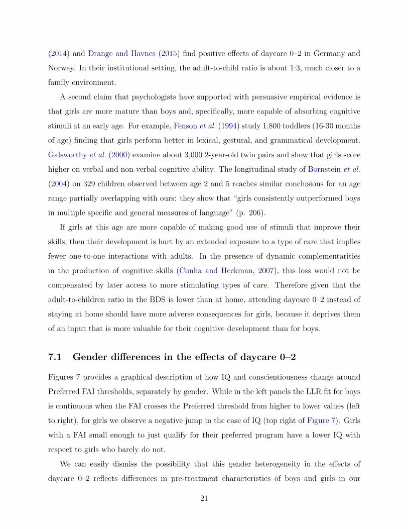
7.1 Gender di↵erences in the e↵ects of daycare 0–2

Figures 7 provides a graphical description of how IQ and conscientiousness change around

Preferred FAI thresholds, separately by gender. While in the left panels the LLR fit for boys

is continuous when the FAI crosses the Preferred threshold from higher to lower values (left

to right), for girls we observe a negative jump in the case of IQ (top right of Figure 7). Girls

with a FAI small enough to just qualify for their preferred program have a lower IQ with

respect to girls who barely do not.

We can easily dismiss the possibility that this gender heterogeneity in the e↵ects of

daycare 0–2 reflects di↵erences in pre-treatment characteristics of boys and girls in our

21

sample: Table 4 as well as previous figures on the continuity of pre-treatment covariates

show that these variables and treatment intensity are perfectly balanced across genders.

Similar across genders are also the answers given by parents to the question concerning

alternative modes of care, which we described above.

We find instead that the evidence for IQ in Figure 7 is confirmed by the parametric

estimation of equation (1), separately for boys and girls. Results are reported in the left

portion of Table 5, for the same three specifications already considered in the corresponding

portion of Table 3. In our preferred specification, which includes all controls in the third

column, the ITT e↵ect of just qualifying for the preferred program, is a statistically significant

loss of about 4.4% of IQ for girls, while for boys it is half as much and we cannot reject the

hypothesis that it is equal to zero. A similar gender di↵erence emerges also in the IV

estimates, which indicate that for girls one additional month in daycare 0–2 reduces IQ by

0.7% (p-value = 0.008), while the e↵ect for boys is about half this size and is not statistically

di↵erent from zero.34 The middle panel shows that the gender gap in the ITT is not due to

di↵erences in the first stage. For both boys and girls, attendance in daycare 0-2 increases

by approximately 6.3 months when the FAI crosses the preferred threshold from higher to

lower values. A qualitatively similar gender di↵erence in the e↵ects of IQ emerges from the

non-parametric estimates reported in columns 2 and 5 of the Appendix Table B where, if

anything, the losses for girls appear to be even larger. The estimates for conscientiousness

are very imprecise in all specifications, parametric or not.

This cognitive loss for girls induced by daycare attendance is a smoking gun for the

relevance of one-to-one interactions with adults as an explanation of our results.35

34Interestingly, in a longitudinal study of 113 first-born preschool children, 58 girls and 55 boys, Bornsteinet al. (2006) find, in line with our results, that “Girls who had greater amount of non-maternal care frombirth to 1 year scored lower on the Spoken Language Quotient at preschool” (pag. 145).

35We have also explored the possibility that the loss su↵ered by girls depend on sex ratios within eachprogram. Psychologists have observed that in early education “(T)eachers spend more time socializing boysinto classroom life, and the result is that girls get less teacher attention. Boys receive what they need ...Girls’ needs are more subtle and tend to be overlooked.” (Koch, 2003, p. 265). However, we do not findany evidence that sex ratios a↵ect the size of the e↵ects for girls and boys, possibly because the variationin these ratios is quite small for the children in our sample. Moreover, the data do not support anotherpossible hypothesis according to which gender di↵erences in breastfeeding explain the gender gap in thee↵ects of daycare. The duration of breastfeeding has been shown to be positively associated with cognitiveoutcomes (Anderson et al., 1999; Borra et al., 2012; Fitzsimons and Vera-Hernandez, 2013), and early daycareenrolment or attendance may shorten it. However, we find no e↵ect (and specifically no di↵erential e↵ect bygender) of days in daycare on breastfeeding duration.

22

7.2 The role of family background

To further support the interpretation suggested in the previous section, we investigate

whether the gender di↵erences in the e↵ect of daycare 0–2 become more evident when one-to-

one interactions at home are complemented by a richer set of cultural and economic resources

o↵ered by a more a✏uent family background.

We explore the role of resources at home by separating children in two groups according

to whether the preferred threshold to which they are associated is above or below the median

of all preferred thresholds.36 Results are reported in Table 6 for girls only and for girls and

boys together.37 Estimates in the left portion of the table are for the less a✏uent group,

and refer to the e↵ect of daycare 0–2 around a preferred threshold of e16.4K on average,

while in the right portion the focus is on the more a✏uent group, around a threshold of

about e33.0K. When the outcome is IQ, in the top panel, girls from more a✏uent families

appear to su↵er a quite large 1.6% loss for every additional month of daycare 0–2. When

all children are considered together the loss drops to 1.1%, suggesting that daycare 0–2

attendance is particularly detrimental for girls with a more favorable home environment.

The point estimate for less a✏uent girls is essentially zero, although with a relatively large

standard error. Interestingly, also in the case of conscientiousness we now see a consistently

negative e↵ect of time spent in daycare 0-2 for girls in a✏uent families, although standard

errors are again large.

8 Conclusions

To the best of our knowledge, this is the first paper that studies the e↵ects time spent in

daycare 0–2 for children from advantaged households, like those with two cohabiting parents

in one of the most highly educated and richest Italian cities. For this population as a whole,

our results indicate quantitatively and statistically significant losses only for girls. Moreover,

these losses are even more pronounced when, within this population, we look at children with

more a✏uent parents. These are typically the relevant marginal subjects to be considered

36Cattaneo et al. (2015) recommend this practice in the presence of multiple thresholds.37Given the very small sample size defined by the intersection of gender and type of threshold, the first

stage for boys is not su�ciently precise.

23

in an evaluation of daycare expansions for the worldwide increasing community of families

in which both parents want to work.

Our results seem relevant not only because of their novelty with respect to the literature,

but more importantly because they implicitly support the hypothesis, suggested by psychol-

ogists, according to which the sign and size of the e↵ects of daycare 0–2 are mostly driven by

three factors: whether this early life experience deprives children of one-to-one interactions

with adults at home, by the quality of these interactions and by whether children can make

good use of them.

For the girls of a✏uent families that we have studied, daycare 0–2 has a negative e↵ect

on cognitive outcomes precisely because the adults-to-children ratio in the Bologna Daycare

System is relatively low with respect to the home environment, because the quality of the

interaction at home that the daycare arrangement crowds out is high, and because these girls

are developed enough, at this young age, to exploit high quality interactions with adults that

for boys are not as valuable.

These results suggest that in the design of daycare expansions for children at very early

ages, a careful cost benefit analysis should be performed to evaluate whether the adult-to-

child ratios that would be necessary to avoid negative e↵ects are privately and socially cost

e↵ective with respect to alternative care modes. Moreover, the gender gap in the e↵ects of

daycare 0–2 that we uncover, points to the desirability of some diversification of daycare

activities for boys and girls, based on their respective maturity.

24

9 Appendix

9.1 How the Family A✏uence Index is constructed

The Family A✏uence Index is the ISEE (Indicatore della Situazione Economica Equivalente) whichis used by the Italian public administration to determine access priority and fees for a wide rangeof public services. For the years we consider the index is computed in three steps. First, earningsof all family members living in the household are added to the income from financial activities ina given year. The latter is estimated by applying the average interest rate on 10-year governmentbonds during the previous year to all financial assets held by family members. If the family paysa rent for its primary dwelling, then an allowance of up to about e5,000 is subtracted from thistotal income component. Denote with Iit this total income component.

Second, the net wealth component is the sum of the values of all non-housing assets (at facevalue, except for stocks which are priced at their market value at the end of the previous year), andthe value of the housing stock (register value), net of the maximum between about e50,000 andthe residual value of all mortgage loans for which that stock is a collateral. A further allowanceof up to about e15,000 can be subtracted from the value of non-housing assets. The 20% of suchmeasure of net wealth is the net wealth component that we denote by Wit.

Finally, the resulting total income and net wealth index is adjusted for family size by dividingthe total income and net wealth components by a concave transformation of family size: 1.00 fora single-person household, 1.57 for a two-person household, 2.04 for three members, 2.46 for fourmembers, 2.85 for five members. For households with more than five members, a coe�cient of 0.35is added to the family size factor for each additional member from the sixth onward. The familysize factor is further increased by 0.2 if the household has a single-parent with children below 18,0.2 if the household has two-working-parents , and 0.5 for each family member with a permanentdisability. Denoting with Sit the family size factor, the FAI index is: Yit = (Iit +Wi)/Sit.

9.2 Stacking thresholds and observations at zero distance

Some specific features of our institutional setting need to be clarified in order to explain why wedrop observations at zero distance from thresholds when we center at zero and stack thresholds fordescriptive purposes and to estimate treatment e↵ects non-parametrically. These specific featureshighlight a potential problem of stacking thresholds in RD designs, which may be common to otherrelevant settings but that seems to have been overlooked in the literature. This potential problem issimilar but not identical to the one highlighted by DeChaisemartin and Behaghel (2015), on whichwe come back below.

Consider a simple example with two programs only: “Poor” and “Rich”. The “Poor” programattracts 80% of applications and has a low FAI threshold. The “Rich” program attracts insteadonly 20% of applications and has a high FAI threshold. When we stack thresholds and consider thedistance from each threshold as the running variable, the average of a covariate (e.g. FAI itself) ina neighbourhood of zero distance (but excluding subjects exactly at zero distance) is an average of“Poor” and “Rich” values with weights that are respectively 0.8 and 0.2. At exactly zero distance,instead, there is one observation for each program and therefore the “Poor” and the “Rich” FAIvalues at exactly zero distance are averaged with equal weights of 0.5. Therefore, while the averageof FAI (or of any other pre-treatment covariate) is a continuous function of the distance from thethreshold around zero distance, it is instead discontinuous exactly at zero distance.

Moreover the density around zero distance would be a mixture of the densities around thetwo separate thresholds and this creates further problems if we modify the above simple example

25

allowing for a larger number of programs (as it is the case in our setting). If densities are continuousat the di↵erent thresholds, after centering and stacking them there would be continuity also of thedensity of the distance around zero. However, exactly at zero we would observe a probabilitymass spike because at this value of the distance we would have one observation for each program,corresponding to each threshold. In the real situation analysed in this paper there are 545 programswith rationing in basket 4 and in all of them there is a child with exactly zero distance from thecorrespondent Final threshold, but the probability of observing any other specific value di↵erentthan zero is theoretically null and e↵ectively small because the FAI is a continuous variable.

DeChaisemartin and Behaghel (2015) suggest that observations at exactly zero distance fromthresholds should be dropped independently of whether the analysis is conducted on thresholdsthat are centered at zero and stacked. In their settings subjects are characterised by an intrinsictype: being a “accepter” or a “refuser” of a potential o↵er. While the proportion of accepters iscontinuous around a threshold, it must be exactly one for subjects located precisely at the threshold.Therefore, independently of stacking, these subjects should be dropped from the analysis. Note,however, that given how we use FAI final thresholds to construct a RD design around PreferredFAI thresholds (see Section 4.2), the problem discussed in DeChaisemartin and Behaghel (2015)does not apply to our parametric analysis.

The problem we highlight may also be reminiscent of the “Donut” problem discussed in Barrecaet al. (2015), but has a very di↵erent origin. In that setting, observations at exactly zero distanceare problematic because of heaping and manipulation of the running variable. In our setting, thereis no heaping and manipulation and the problem originates from stacking thresholds in a situationin which:

a in each program the threshold is the value of the running variable corresponding to the lastchild who receives an o↵er and accepts it;

b the running variable is continuous and not uniformly distributed;

c there is a large number of thresholds.

9.3 Continuity of pre-treatment variables

As a further, explicit test of the continuity of pre-treatment covariates, we follow Abdulkadiroluet al. (2014) and estimate a system of 8 equations (one for each covariate xit 2 Xit of equation(1) via Seemingly Unrelated Regression and then we test the joint significance of the instrumentdefined by equation (2) across the system equations. The system is represented by:

xit = ↵+ �Pit + �Ait + f(Yit) + ✏it, (5)

where xit is one of the following: years of father education, years of mother education, father yearof birth, mother year of birth, number of siblings at the time of the first application, whether thefather was self-employed at the time of the first application, whether the mother was self-employedat the time of the first application, whether Cesarean delivery of the child. Table A reports resultsand test statistics. Continuity is never rejected.

26

References

Abdulkadiroglu, A., Angrist, J. D., Narita, Y., Pathak, P. A., 2015, Research design meetsmarket design: Using centralized assignment for impact evaluation, Working Paper 21705,National Bureau of Economic Research.

Abdulkadirolu, A., Angrist, J., Pathak, P., 2014, The Elite Illusion: Achievement E↵ects atBoston and New York Exam Schools, Econometrica 82, 137–196.

Adi-Japha, E., Klein, P. S., 2009, Relations Between Parenting Quality and Cognitive Per-formance of Children Experiencing Varying Amounts of Childcare, Child Development 80,893–906.

Almond, D., Currie, J., 2011, Human Capital Development Before Age Five, volume 4, PartB of Handbook of Labor Economics, 1315 – 1486, Elsevier.

Anderson, J. W., Johnstone, B. M., Remley, D. T., 1999, Breast-feeding and cognitivedevelopment: a meta-analysis, The American Journal of Clinical Nutrition 70, 525–535.

Anderson, M. L., 2008, Multiple Inference and Gender Di↵erences in the E↵ects of EarlyIntervention: A Reevaluation of the Abecedarian, Perry Preschool, and Early TrainingProjects, Journal of the American Statistical Association 103, 1481–1495.

Baker, M., Gruber, J., Milligan, K., 2008, Universal Child Care, Maternal Labor Supply,and Family Well-Being, Journal of Political Economy 116, 709–745.

Baker, M., Gruber, J., Milligan, K., 2015, Non-Cognitive Deficits and Young Adult Out-comes: The Long-Run Impacts of a Universal Child Care Program, Working Paper 21571,National Bureau of Economic Research.

Barreca, A. I., Lindo, J. M., Waddell, G. R., 2015, Heaping-Induced Bias in Regression-Discontinuity Designs, Economic Inquiry .

Bernal, R., Keane, M. P., 2011, Child Care Choices and Children’s Cognitive Achievement:The Case of Single Mothers, Journal of Labor Economics 29, pp. 459–512.

Borghans, L., Duckworth, A. L., Heckman, J. J., ter Weel, B., 2008, The Economics andPsychology of Personality Traits, Journal of Human Resources 43, 972–1059.

Bornstein, M., Hahn, C.-S., Gist, N., Haynes, M., 2006, Long term cumulative e↵ects ofchildcare on children’s mental development and socioemotional adjustment in a non-risksample: the moderating e↵ects of gender, Early Child Development and Care 176, 129–156.

Bornstein, M. H., Hahn, C.-S., Haynes, O. M., 2004, Specific and general language perfor-mance across early childhood: Stability and gender considerations, First Language 24,267–304.

Borra, C., Iacovou, M., Sevilla, A., 2012, The e↵ect of breastfeeding on children’s cognitiveand noncognitive development , Labour Economics 19, 496 – 515.

27

Brooks-Gunn, Jeanne, W.-J. H., Waldfogel, J., 2002, Maternal Employment and Child Cog-nitive Outcomes in the First Three Years of Life: The NICHD Study of Early Child Care,Child Development 73, 1052?1072.

Calonico, S., Cattaneo, M. D., Titiunik, R., 2014a, Robust Data Driven Inference in theRegression-Discontinuity Design, The Stata Journal 14, 909–946.

Calonico, S., Cattaneo, M. D., Titiunik, R., 2014b, Robust Nonparametric Confidence In-tervals for Regression-Discontinuity Designs, Econometrica 82, 2295–2326.

Campbell, F. A., Ramey, C. T., 1994, E↵ects of Early Intervention on Intellectual andAcademic Achievement: A Follow-up Study of Children from Low-Income Families, ChildDevelopment 65, 684–698.

Carneiro, P., Cunha, F., Heckman, J., 2003, Interpreting The Evidence of Family Influenceon Child Development, Mimeo.

Carneiro, P., Ginja, R., 2014, Long-Term Impacts of Compensatory Preschool on Healthand Behavior: Evidence from Head Start, American Economic Journal: Economic Policy6, 135–73.

Carneiro, P., Lken, K. V., Salvanes, K. G., 2015, A Flying Start? Maternity Leave Benefitsand Long-Run Outcomes of Children, Journal of Political Economy 123, pp. 365–412.

Cartmill, E., Armstrong, B., Gleitman, L., Goldin-Meadow, S., Medina, T., Trueswell, J.,2013, Quality of early parent input predicts child vocabulary 3 years later, PNAS 110, pp.11278–11283.

Cattaneo, M., Keele, L., Titiunik, R., Vazquez-Bare, G., 2015, Interpreting Regression Dis-continuity Designs with Multiple Cuto↵s, Mimeo.

Clarke-Stewart, K., Gruber, C., Fitzgerald, L., 1994, Children at home and in day care , L.Erlbaum Associates, Hillsdale, NJ.

Csibra, G., Gergely, G., 2009, Natural Pedagogy, Philosophical Transactions of the RoyalSociety B 13, 148–153.

Csibra, G., Gergely, G., 2011, Natural Pedagogy as evolutionary adaptation, Trends inCognitive Sciences 366, 1149–1157.

Cunha, F., Heckman, J., 2007, The Technology of Skill Formation, American EconomicReview 97, 31–47.

Currie, J., 2001, Early Childhood Education Programs, Journal of Economic Perspectives15, 213–238.

DeChaisemartin, C., Behaghel, L., 2015, Next please! A new definition of the treatment andcontrol groups for randomizations with waiting lists, Mimeo.

Del Boca, D., Pronzato, C., Sorrenti, G., 2015, When rationing plays a role: selection criteriain the Italian early child care system, Carlo Alberto Notebooks 399, Collegio Carlo Alberto.

28

Drange, N., Havnes, T., 2015, Child Care Before Age Two and the Development of Languageand Numeracy: Evidence from a Lottery, IZA Discussion Papers 8904, Institute for theStudy of Labor (IZA).

Duncan, G. J., Magnuson, K., 2013, Investing in Preschool Programs, Journal of EconomicPerspectives 27, 109–32.

Dustmann, C., Raute, A., Schonberg, U., 2013, Does Universal Child Care Matter? Evidencefrom a Large Expansion in Pre-School Education, Mimeo.

Elango, S., Garca, J. L., Heckman, J. J., Hojman, A., 2015, Early childhood education,Working Paper 21766, National Bureau of Economic Research.

Felfe, C., Lalive, R., 2014, Does Early Child Care Help or Hurt Childrens’s Development?,IZA Discussion Papers 8484, Institute for the Study of Labor (IZA).

Felfe, C., Nollenberger, N., Rodrguez-Planas, N., 2015, Cant Buy Mommys Love? Univer-sal Childcare and Children’s Long-Term Cognitive Development, Journal of PopulationEconomics 28, 393–422.

Fenson, L., Dale, P. S., Reznick, J. S., Bates, E., Thal, D. J., Pethick, S. J., Tomasello,M., Mervis, C. B., Stiles, J., 1994, Variability in Early Communicative Development,Monographs of the Society for Research in Child Development 59, pp. i+iii–v+1–185.

Fitzsimons, E., Vera-Hernandez, M., 2013, Food for Thought? Breastfeeding and ChildDevelopment, IFS Working Papers (W13/31).

Gale, D., Shapley, L., 1962, College Admissions and the Stability of Marriage, AmericanMathematical Monthly 69, pp. 9–15.

Galsworthy, M. J., Dionne, G., Dale, P. S., Plomin, R., 2000, Sex di↵erences in early verbaland non-verbal cognitive development, Developmental Science 3, 206–215.

Garber, H., 1988, The Milwaukee Project: Preventing Mental Retardation in Children AtRisk, Technical report, American Association on Mental Retardation.

Gottfredson, L. S., 1997, Mainstream science on intelligence: An editorial with 52 signatories,history, and bibliography, Intelligence 24, 13 – 23, special Issue Intelligence and SocialPolicy.

Gunderson, E. A., Gripshover, S. J., Romero, C., Dweck, C. S., Goldin-Meadow, S., Levine,S. C., 2013, Parent praise to 1- to 3-year-olds predicts children’s motivational frameworks5 years later, Child Development 84, 1526–1541.

Hart, B., Risley, T., 1995, Meaningful Di↵erences in the Everyday Experience of YoungAmerican Children , Brookes Publishing Co., Baltimore MD.

Havnes, T., Mogstad, M., 2015, Is Universal Child Care Leveling the Playing Field?, Journalof Public Economics 127, 100 – 114.

Heckman, J. J., Mosso, S., 2014, The Economics of Human Development and Social Mobility,Annual Review of Economics 27, 109–32.

29

Herbst, C. M., 2013, The Impact of Non-Parental Child Care on Child Development: Evi-dence from the Summer Participation Dip, Journal of Public Economics 105, 86 – 105.

Hewett, V., 2001, Examining the Reggio Emilia Approach to Early Childhood Education,Early Childhood Education Journal 29, 95–100.

Imbens, G. W., Lemieux, T., 2008, Regression discontinuity designs: A guide to practice,Journal of Econometrics 142, 615–635.

Kottelenberg, M. J., Lehrer, S. F., 2014a, Do the perils of universal childcare depend on thechilds age?, CESifo Economic Studies 60, 338–365.

Kottelenberg, M. J., Lehrer, S. F., 2014b, The Gender E↵ects of Universal Child Care inCanada: Much ado about Boys?, Mimeo.

Lee, D. S., Lemieux, T., 2010, Regression discontinuity designs in economics, Journal ofEconomic Literature 48, 281–355.

Li, J., Johnson, S. E., Han, W.-J., Andrews, S., Kendall, G., Strazdins, L., Dockery, A.,2013, Parents’ nonstandard work schedules and child well-being: A critical review of theliterature, The Journal of Primary Prevention 35, 53–73.

Magnuson, K. A., Ruhm, C., Waldfogel, J., 2007, Does prekindergarten improve schoolpreparation and performance?, Economics of Education Review 26, 33–51.

McCrary, J., 2008, Manipulation of the Running Variable in the Regression DiscontinuityDesign: A Density Test, Journal of Econometrics 142, 698–714.

McPherran Lombardi, C., Levine Coley, R., 2014, Early Maternal Employment and ChildrensSchool Readiness in Contemporary Families, Developmental Psychology 50, 2071–2084.

Noboa-Hidalgo, G. E., Urza, S. S., 2012, The E↵ects of Participation in Public Child CareCenters: Evidence from Chile, Journal of Human Capital 6, 1 – 34.

Puma, M., Bell, S., Cook, R., Heid, C., Broene, P., Jenkins, F., Mashburn, A., Downer, J.,2012, Third Grade Follow-up to the Head Start Impact Study Final Report, OPRE Report2012-45, Washington, DC: O�ce of Planning, Research and Evaluation, Administrationfor Children and Families, U.S. Department of Health and Human Services.

Roth, A. E., 2007, Deferred acceptance algorithms: History, theory, practice, and openquestions, Working Paper 13225, National Bureau of Economic Research.

Rowe, M. L., Goldin-Meadow, S., 2009, Di↵erences in early gesture explain SES disparitiesin child vocabulary size at school entry, Science 323, 951–953.

Zigler, E., Butterfield, E. C., 1968, Motivational Aspects of Changes in IQ Test Performanceof Culturally Deprived Nursery School Children, Child Development 39, pp. 1–14.

30

Figures and Tables

Figure 1: Persistence of Final FAI thresholds and Basket 4 vacancies over time

010

020

030

0th

resh

old

in y

ear t

0 100 200 300threshold in year t-1

Final FAI thresholds

010

2030

B4 v

acan

cies

in y

ear t

0 10 20 30B4 vacancies in year t-1

Basket 4 vacancies

Notes: Each dot represents a program and the coordinates are either the Final FAI thresholds of that program in two consecutive

years (left panel), or the vacant capacity for “basket 4” (two working parents) children in two consecutive years (right panel).

FAI stands for Family A✏uence Index. Sample: 238 programs with rationing for “basket 4” children in two consecutive years.

The lack of persistence of Final FAI thresholds is of course even more evident for programs that are not o↵ered every year.

31

Figure 2: Density of distance and continuity around Final FAI thresholds

0.0

2.0

4.0

6D

ensi

ty

-50 -40 -30 -20 -10 0 10 20 30 40 50

130

170

210

Birth

day

-50 -40 -30 -20 -10 0 10 20 30 40 50

025

5075

FAI

-50 -40 -30 -20 -10 0 10 20 30 40 50

1415

16N

eigh

b. in

com

e

-50 -40 -30 -20 -10 0 10 20 30 40 50

01

Sibl

ings

-50 -40 -30 -20 -10 0 10 20 30 40 507

10Pr

efer

ence

s

-50 -40 -30 -20 -10 0 10 20 30 40 50

Boys Girls

Notes: The dots represent the frequency distribution (top-left panel) and the average of five pre-treatment variables (remaining

panels) inside e2000 bins, plotted as a function of the distance (thousands of real e) of a child’s FAI from her Final FAI

threshold, by gender. The bold lines are LLR on the underlying individual observations, with a triangular kernel and optimal

bandwidth selection, from Calonico et al. (2014b). FAI stands for Family A✏uence Index. Sample: 5,089 children with two

working parents, born between 1999 and 2005 who first applied for admission between 2001 and 2005, whose FAI distance from

the Final FAI thresholds is at most e50K and is di↵erent from zero.

32

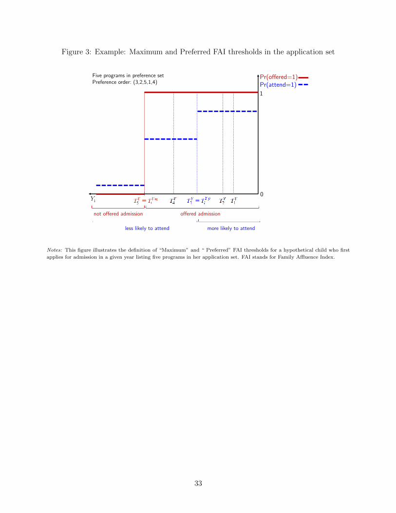
Figure 3: Example: Maximum and Preferred FAI thresholds in the application set

Yi 0

1

Pr(offered=1) Pr(attend=1)

offered admission not offered admission

more likely to attend less likely to attend

Five programs in preference set Preference order: (3,2,5,1,4)

Notes: This figure illustrates the definition of “Maximum” and “ Preferred” FAI thresholds for a hypothetical child who first

applies for admission in a given year listing five programs in her application set. FAI stands for Family A✏uence Index.

33

Figure 4: Admission o↵ers and attendance around Preferred FAI thresholds

0.1

.2.3

.4.5

.6.7

.8.9

1Ad

mis

sion

rate

-50 -25 0 25 50distance from FAI threshold

0.1

.2.3

.4.5

.6.7

.8.9

1At

tend

ance

rate

-50 -25 0 25 50distance from FAI threshold

050

100

150

200

250

300

350

Day

s of

atte

ndan

ce a

t age

0-2

-50 -25 0 25 50distance from FAI threshold

Boys Girls

Notes: The dots represent o↵er rates (left), attendance rates (middle) and average days of attendance at age 0–2 (right) inside

e2000 bins, plotted as a function of the distance (thousands of real e) of a child’s FAI from her Preferred FAI threshold, by

gender. The bold lines are LLR on the underlying individual observations, with a triangular kernel and optimal bandwidth

selection, from Calonico et al. (2014b). FAI stands for Family A✏uence Index. Sample: 5,101 children with two working

parents, born between 1999 and 2005 who first applied for admission between 2001 and 2005, whose FAI distance from the

Preferred FAI threshold is at most e50K and is di↵erent from zero.

34

Figure 5: Density of distance and continuity of covariates around Preferred FAI thresholds

0.0

2.0

4.0

6

-50 -40 -30 -20 -10 0 10 20 30 40 50

100

175

250

Birth

day

-50 -40 -30 -20 -10 0 10 20 30 40 50

025

5075

FAI

-50 -40 -30 -20 -10 0 10 20 30 40 50

1214

16N

eigh

b. in

com

e

-50 -40 -30 -20 -10 0 10 20 30 40 50

01

Sibl

ings

-50 -40 -30 -20 -10 0 10 20 30 40 50

05

10Pr

efer

ence

s

-50 -40 -30 -20 -10 0 10 20 30 40 50

Boys Girls

Notes: The dots represent the frequency distribution (top-left panel) and the average of five pre-treatment variables (remaining

panels) inside e2000 bins, plotted as a function of the distance (thousands of real e) of a child’s FAI from her Preferred FAI

threshold, by gender. The bold lines are LLR on the underlying individual observations, with a triangular kernel and optimal

bandwidth selection, from Calonico et al. (2014b). FAI stands for Family A✏uence Index. Sample: 5,101 children with two

working parents, born between 1999 and 2005 who first applied for admission between 2001 and 2005, whose FAI distance from

the Preferred FAI thresholds is at most e50K and is di↵erent from zero.

35

Figure 6: Interviews and response rates around Preferred FAI thresholds

0.2

.4.6

.81

-50 -25 0 25 50distance from FAI threshold

Boys Girls

invitation rate of universe

0.2

.4.6

.81

-50 -25 0 25 50distance from FAI threshold

Boys Girls

response rate of invited

0.2

.4.6

.81

-50 -25 0 25 50distance from FAI threshold

Boys Girls

interview rate of universe0

510

1520

25

-50 -25 0 25 50distance from FAI threshold

Universe not invitedInvited

Frequency0

24

68

10

-50 -25 0 25 50distance from FAI threshold

Invited not interviewedInterviewed

Frequency

05

1015

2025

-50 -25 0 25 50distance from FAI threshold

Universe not interviewedInterviewed

Frequency

Notes: The top row shows the continuity of the invitation rate for the universe (left), the response rate of the invited (middle),

and the interview rate for the universe (right) at the Preferred FAI threshold, by gender, as a function of the distance from

the threshold, meausured in thousands of real e. The bold lines are LLR on the underlying individual observations, with a

triangular kernel and optimal bandwidth selection, from Calonico et al. (2014b). The bottom row shows the absolute frequency

distribution of children in the universe (left and right) and the invited (middle), and, on top of each bar, the corresponding

distribution of invited (left) and interviewed children (middle and right) inside e2000 bins, plotted as a function of the distance

(thousands of real e) of a child’s FAI from her Preferred FAI threshold, by gender. FAI stands for Family A✏uence Index.

Sample: 5,101 children with two working parents, born between 1999 and 2005 who first applied for admission between 2001

and 2005, whose FAI distance from the Preferred FAI thresholds is at most e50K and is di↵erent from zero.

36

Figure 7: Full Scale IQ and Conscientiousness around Preferred FAI thresholds, by gender

9010

011

012

013

014

0

-50 -40 -30 -20 -10 0 10 20 30 40 50distance from FAI threshold

Boys

9010

011

012

013

014

0

-50 -40 -30 -20 -10 0 10 20 30 40 50distance from FAI threshold

Girls

Full Scale IQ

1020

3040

5060

70

-50 -40 -30 -20 -10 0 10 20 30 40 50distance from FAI threshold

Boys

1020

3040

5060

70

-50 -40 -30 -20 -10 0 10 20 30 40 50distance from FAI threshold

Girls

Conscientiousness

Notes: The dots represent average IQ (top panels) and average Conscientiousness (bottom panels) inside e2000 bins, plotted

as a function of the distance (thousands of real e) of a child’s FAI from her Preferred FAI threshold, by gender. The bold lines

are LLR on the underlying individual observations, with a triangular kernel and optimal bandwidth selection, from Calonico

et al. (2014b). FAI stands for Family A✏uence Index. Sample: 373 (top panels) and 371 (bottom panels) interviewed children

with two working parents, born between 1999 and 2005 who first applied for admission between 2001 and 2005, whose FAI

distance from the Preferred FAI thresholds is at most e50K and is di↵erent from zero.

37

Table 1: Descriptive statistics for the basket 4 universe, the invited and the interview samples

Variable Universe B4 Invited Interview p-val

FAI at first application 24.87 26.50 27.10 0.007(20.50) (19.70) (17.55) [0.547]

{0.010}Number of preferences at first application 5.42 5.29 5.59 0.222

(3.66) (3.42) (3.53) [0.120]{0.341}

Siblings at first application 0.48 0.49 0.54 0.755(0.66) (0.65) (0.70) [0.151]

{0.079}Day of birth in the year 182.8 186.6 180.5 0.222

(104.1) (106.) (111.1) [0.310]{0.673}

O↵ered admission at first application 0.897 0.777 0.752 0.000(0.303) (0.417) (0.432) [0.297]

{0.000}Waiver at first application 0.124 0.075 0.068 0.000

(0.330) (0.263) (0.251) [0.607]{0.000}

Year first applied 2003.1 2003.4 2003.5 0.000(1.43) (1.42) (1.38) [0.086]

{0.000}Year child born 2002.0 2002.5 2002.6 0.000

(1.58) (1.63) (1.62) [0.086]{0.000}

Grade first applied for 0.882 0.568 0.540 0.000(0.786) (0.673) (0.676) [0.459]

{0.000}Days in 212.2 223.6 230.5 0.010

(143.3) (151.4) (156.3) [0.417]{0.017}

Ever attended (share with days in >0) 0.847 0.784 0.782 0.000(0.360) (0.411) (0.414) [0.916]

{0.001}

N 6,575 1,379 444

Notes: This table compares the means of variables from the administrative records in the “basket 4” (B4) universe (6,575

children whose parents were both employed at the time of the first application, born between 1999 and 2005 who first applied

for admission between 2001 and 2005), in the sample invited for an interview (1,379 children sampled from this universe), and

in the interview sample (444 children sampled and interviewed from the universe). The p-values in the last column refer to

tests of the equality of means for the B4 universe and the invited (first row), the invited and the interviewed (second row, in

square brackets), the B4 universe and the interviewed (third row, in curly brackets). FAI stands for Family A✏uence Index.

38

Table 2: The interviewed sample in comparison to the Northern Italian population

Interview sample Northern Italy

Child age 10.7 11.1(1.6) (1.7)

Father age 47.3 47.0(4.8) (4.7)

Mother age 44.9 45.0(4.1) (4.8)

Years education father 14.2 13.1(3.8) (3.0)

Years education mother 15.5 14.4(3.2) (2.5)

Father self-employed 0.236 0.276(0.425) —

Mother self-employed 0.106 0.173(0.308) —

Observations 444 93

Notes: This table compares the means of variables in the interview sample with the corresponding means in the Bank of

Italy Survey of Household Income and Wealth (SHIW – age, education) and in the Labor Force Statistics (ISTAT – parental

occupation). The SHIW is restricted to households with two employed parents from the 2000, 2002, 2004, and 2006 waves,

living in cities of Northern Italy with a population of at least 200,000, and who between 2013 and 2015 have at least one child

between 8 and 14 years of age. The Labor Force Statistics refer to year 2005, and to workers between 25 and 44 years of age

(i.e., the age range of parents in our sample when they first applied for daycare admission 8 to 12 years prior to the interview.)

39

Table 3: E↵ects of daycare attendance on IQ and Conscientiousness for all children

Log of IQ Log of Conscientiousness

ITT e↵ect of qualifying -0.026* -0.030** -0.031** -0.001 0.005 0.006for the preferred program (0.011) (0.011) (0.011) (0.024) (0.025) (0.024)

First stage: e↵ect of qualifying 6.3** 6.4** 6.2** 6.3** 6.4** 6.2**on months of attendance (0.9) (0.9) (0.9) (0.9) (0.9) (0.9)

IV e↵ect of one month -0.004* -0.005** -0.005** -0.000 0.001 0.001of daycare attendance (0.002) (0.002) (0.002) (0.004) (0.004) (0.004)

F-stat on excluded instruments 53.8 51.4 46.1 53.1 51.0 46.0Number of observations 444 444 444 441 441 441

Polynomial in FAI Yes Yes Yes Yes Yes YesAppl. set controls Yes Yes Yes YesPre-treat. controls Yes Yes

Notes: Parametric estimates of the e↵ect of one month of daycare 0–2 on the log of IQ and the log of Conscientiousness, with

related ITT and first stage. ITT coe�cients derive from regressions of the outcome on the instrument (whether the child’s

qualifies for the preferred program) and controls as in equation (3). First-stage coe�cients derive from regressions of months

spent in daycare 0–2 on the instrument and controls as in equation (4). IV coe�cients derive from regressions of the outcome

on months of attendance and controls, as in equation (1), using a dummy for qualification in the preferred program as the

instrument. The running variable is the Family A✏uence Index (FAI). The polynomial in the running variable is of second

order. Sample: interviewed children with two working parents, born between 1999 and 2005, with non missing outcome or

covariates and who first applied for admission between 2001 and 2005. Robust standard errors in parentheses, clustered at the

facility level. * significant at 5%; ** significant at 1% or better.

40

Tab

le4:

Characteristicsof

interviewed

boysan

dgirls

Boys

Girls

p-val

Boys

Girls

p-val

FAI

27.3

26.9

0.82

Father

education

inyears

14.1

14.4

0.49

(1.3)

(1.1)

(0.26)

(0.24)

N.of

preferences

5.46

5.71

0.46

Mother

education

inyears

15.5

15.4

0.82

(0.24)

(0.23)

(0.22)

(0.21)

N.of

siblings

1.56

1.53

0.66

Father

birthyear

1966.3

1966.2

0.81

(0.05)

(0.05)

(0.32)

(0.32)

O↵ered

admission

0.76

0.75

0.78

Mother

birth

year

1968.5

1968.6

0.85

(0.03)

(0.03)

(0.27)

(0.28)

Waiver

0.05

0.08

0.18

Father

self-employed

0.24

0.23

0.80

(0.02)

(0.02)

(0.03)

(0.03)

Yearof

firstap

plication

2003.4

2003.6

0.18

Mother

self-employed

0.11

0.10

0.70

(0.09)

(0.09)

(0.02)

(0.02)

Gradeat

firstap

plication

1.57

1.52

0.42

Cesareandelivery

0.30

0.24

0.14

(0.05)

(0.04)

(0.03)

(0.03)

Everattended

0.78

0.78

0.99

Mon

thof

breastfeeding

6.45

6.12

0.45

(0.03)

(0.03)

(0.30)

(0.32)

Mon

thsat

entry

15.2

15.0

0.79

Interviewer:psychologist1

0.433

0.384

0.30

(0.5)

(0.5)

(0.03)

(0.03)

Daysof

attendan

ce229.8

231.1

0.93

Interviewer:psychologist2

0.163

0.179

0.65

(10.5)

(10.5)

(0.03)

(0.03)

Yearborn

2002.5

2002.7

0.21

Interviewer:psychologist3

0.400

0.432

0.49

(0.11)

(0.11)

(0.03)

(0.03)

Day

born

177.4

183.4

0.57

Yearinterviewed

2013.7

2013.7

0.43

(7.5)

(7.4)

(0.04)

(0.04)

Age

atinterview

10.7

10.6

0.31

Mon

thinterviewed

7.1

7.0

0.69

(0.11)

(0.10)

(0.2)

(0.2)

Notes:This

table

comparesth

e215boy

sand229girls

ofth

einterview

sample

(444ch

ildrenwithtw

oworkingparents).

Forea

chva

riable

andgen

der

thetable

reportsth

e

mea

n,th

estandard

dev

iation

inparenth

esis

and

thep-valueofatest

thatth

emea

nis

equalforboy

sand

girls.Thesourceforparentalback

ground,typeofdelivery,

and

breastfeed

ingare

theinterviews.

Forallth

eoth

erva

riablesth

esourceis

theadministrativedatasetofth

eBDS.FAIstandsforFamilyA✏uen

ceIndex

.

41

Table 5: Gender heterogeneity of the e↵ects of daycare 0–2 on IQ and Conscientiousness

Log of IQ Log of Conscientiousness

ITT e↵ect of qualifying for the preferred program

Girls -0.040** -0.043** -0.044** 0.006 0.012 0.022(0.015) (0.016) (0.016) (0.035) (0.036) (0.037)

Boys -0.013 -0.018 -0.022 -0.006 0.003 0.004(0.016) (0.016) (0.015) (0.036) (0.037) (0.036)

First stage e↵ect of qualifying on months of attendance

Girls 6.54** 6.42** 6.36** 6.54** 6.42** 6.36**(1.13) (1.19) (1.20) (1.13) (1.19) (1.20)

F-stat excl. instr. 33.4 29.3 27.9 33.4 29.3 27.9

Boys 6.11** 6.68** 6.23** 6.11** 6.71** 6.26**(0.92) (0.88) (0.90) (0.93) (0.89) (0.91)

F-stat excl. instr. 44.3 57.2 47.6 43.1 56.4 47.5

IV e↵ect of one month of daycare attendance

Girls -0.006* -0.007* -0.007** 0.001 0.002 0.003(0.002) (0.003) (0.003) (0.005) (0.005) (0.006)

Boys -0.002 -0.003 -0.004 -0.001 0.000 0.001(0.003) (0.002) (0.002) (0.006) (0.005) (0.005)

Polynomial in FAI Yes Yes Yes Yes Yes YesAppl. set controls Yes Yes Yes YesPre-treat. controls Yes Yes

Notes: Parametric estimates by gender of the e↵ect of one month of daycare 0–2 on the log of IQ and the log of Conscientiousness,

with related ITT and first stage. ITT coe�cients derive from regressions of the outcome on the instrument (whether the child’s

qualifies for the preferred program) and controls as in equation (3). First-stage coe�cients derive from regressions of months

spent in daycare 0–2 on the instrument and controls as in equation (4). IV coe�cients derive from regressions of the outcome

on months of attendance and controls, as in equation (1), using a dummy for qualification in the preferred program as the

instrument. The running variable is the Family A✏uence Index (FAI). The polynomial in the running variable is of second

order. Sample: interviewed children with two working parents, born between 1999 and 2005, with non missing corresponding

outcome or covariates and who first applied for admission between 2001 and 2005. Number of observations: 229 girls for both IQ

and Conscientiousness; 215 boys for IQ and 212 for Conscientiousness (see footnote 23). Robust standard errors in parentheses,

clustered at the facility level. * significant at 5%; ** significant at 1% or better.

42

Table 6: E↵ects of one month of daycare 0–2 by level of the Preferred FAI threshold

Threshold median Threshold > median(mean treshold: e16.4K) (mean treshold: e33.0K)

Log of IQ

Girls -0.000 -0.001 -0.001 -0.016** -0.016** -0.016*(0.003) (0.003) (0.003) (0.006) (0.005) (0.007)

Boys & Girls -0.001 -0.002 -0.001 -0.011* -0.011* -0.011*(0.004) (0.003) (0.003) (0.005) (0.005) (0.005)

Log of Conscientiousness

Girls 0.011 0.007 0.009 -0.018 -0.019 -0.019(0.009) (0.008) (0.007) (0.013) (0.012) (0.013)

Boys & Girls 0.004 0.006 0.006 -0.014 -0.013 -0.015(0.007) (0.006) (0.007) (0.011) (0.010) (0.012)

Poly. FAI Yes Yes Yes Yes Yes YesApp. set Yes Yes Yes YesPre-treat. Yes Yes

Notes: Parametric IV estimates of the e↵ect of one month of daycare 0–2 on the log of IQ and the log of Conscientiousness,

separately for Preferred FAI thresholds below or above the median Fai threshold. Coe�cients derive from regressions of the

outcome on months of attendance and controls, as in equation (1), using a dummy for qualification in the preferred program as

the instrument. The first stage for boys is not su�ciently precise below the median. We therefore present, for each outcome,

estimates for girls only and for girls and boys together. The running variable is the Family A✏uence Index (FAI). The polynomial

in the running variable is of second order. Sample: interviewed children with two working parents, born between 1999 and 2005,

with non missing corresponding outcome or covariates and who first applied for admission between 2001 and 2005. Number

of observations: 108 girls below the median and 104 girls above in the case of both IQ and Conscientiousness; 204 children

below the median and 204 children above in the case of IQ; 203 children below the median and 203 children above in the case

of conscientiousness. Robust standard errors in parentheses, clustered at the facility level. * significant at 5%; ** significant at

1% or better.

43

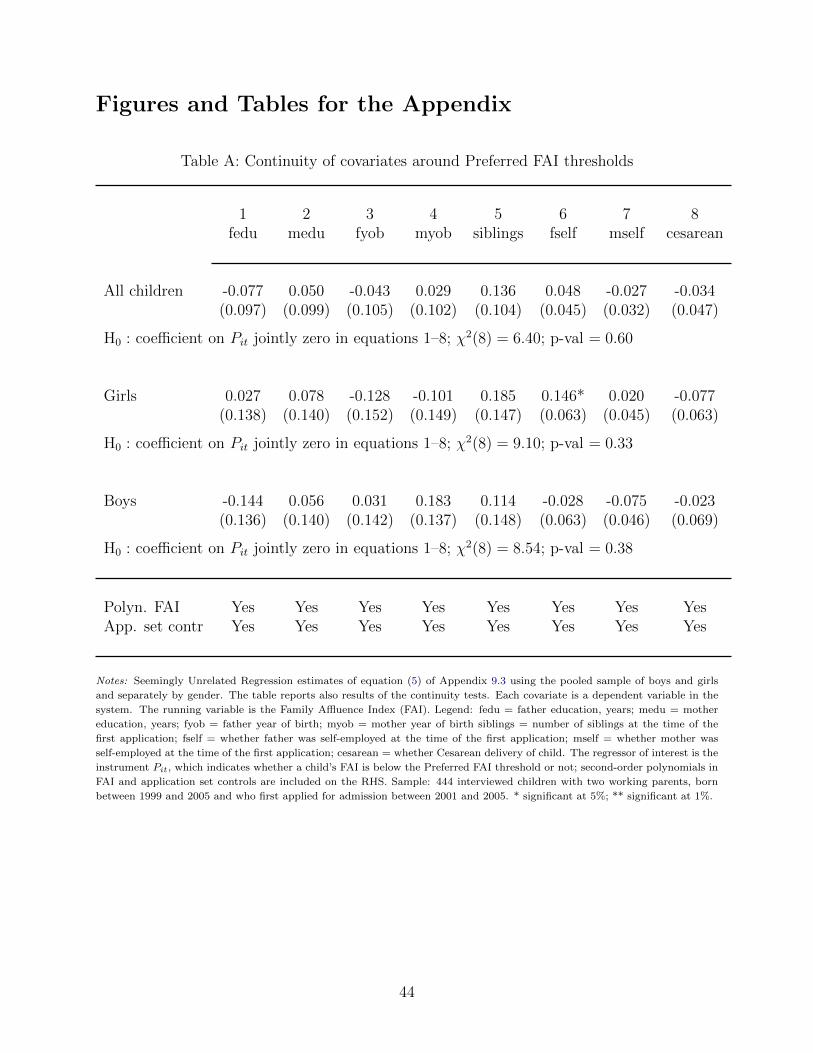
Figures and Tables for the Appendix

Table A: Continuity of covariates around Preferred FAI thresholds

1 2 3 4 5 6 7 8fedu medu fyob myob siblings fself mself cesarean

All children -0.077 0.050 -0.043 0.029 0.136 0.048 -0.027 -0.034(0.097) (0.099) (0.105) (0.102) (0.104) (0.045) (0.032) (0.047)

H0 : coe�cient on Pit jointly zero in equations 1–8; �2(8) = 6.40; p-val = 0.60

Girls 0.027 0.078 -0.128 -0.101 0.185 0.146* 0.020 -0.077(0.138) (0.140) (0.152) (0.149) (0.147) (0.063) (0.045) (0.063)

H0 : coe�cient on Pit jointly zero in equations 1–8; �2(8) = 9.10; p-val = 0.33

Boys -0.144 0.056 0.031 0.183 0.114 -0.028 -0.075 -0.023(0.136) (0.140) (0.142) (0.137) (0.148) (0.063) (0.046) (0.069)

H0 : coe�cient on Pit jointly zero in equations 1–8; �2(8) = 8.54; p-val = 0.38

Polyn. FAI Yes Yes Yes Yes Yes Yes Yes YesApp. set contr Yes Yes Yes Yes Yes Yes Yes Yes

Notes: Seemingly Unrelated Regression estimates of equation (5) of Appendix 9.3 using the pooled sample of boys and girls

and separately by gender. The table reports also results of the continuity tests. Each covariate is a dependent variable in the

system. The running variable is the Family A✏uence Index (FAI). Legend: fedu = father education, years; medu = mother

education, years; fyob = father year of birth; myob = mother year of birth siblings = number of siblings at the time of the

first application; fself = whether father was self-employed at the time of the first application; mself = whether mother was

self-employed at the time of the first application; cesarean = whether Cesarean delivery of child. The regressor of interest is the

instrument Pit, which indicates whether a child’s FAI is below the Preferred FAI threshold or not; second-order polynomials in

FAI and application set controls are included on the RHS. Sample: 444 interviewed children with two working parents, born

between 1999 and 2005 and who first applied for admission between 2001 and 2005. * significant at 5%; ** significant at 1%.

44

Table B: E↵ect of daycare 0–2 on IQ and Conscientiousness: non-parametric estimates.

Gender All Girls Boys All Girls Boys

Log of IQ Log of Conscientiousness

ITT of just -0.028 -0.037 -0.011 0.037 0.059 0.009qualifying (0.020) (0.026) (0.041) (0.048) (0.072) (0.043)

First stage 4.6** 3.75* 6.2* 4.1* 2.7 6.2*(1.3) (1.6) (2.6) (1.5) (1.9) (2.4)

robust p-value 0.045 0.485 0.055 0.083 0.784 0.060

E↵ect of 1 month -0.006 -0.010 -0.002 0.009 0.022 0.001(conventional) (0.005) (0.008) (0.007) (0.012) (0.028) (0.007)

E↵ect of 1 month -0.006 -0.015+ -0.001 0.015 0.048+ 0.002(bias-corrected) (0.005) (0.008) (0.007) (0.012) (0.028) (0.007)

E↵ect of 1 month -0.006 -0.015 -0.001 0.015 0.048 0.002(robust) (0.006) (0.011) (0.009) (0.015) (0.036) (0.009)

Bandwith for Loc. Poly (h) 6.544 7.076 5.088 5.023 4.985 6.170Bandwith for bias (b) 16.351 16.297 10.820 12.815 13.382 14.304Number of observations 150 91 46 115 70 57

Notes: Non-parametric estimates of the e↵ect of one month of daycare 0–2 on the log of IQ and the log of Conscientiousness,

with related ITT and first stage. We follow the methodology suggested in Calonico et al. (2014b) and use their software

described in Calonico et al. (2014a). The grade of local polynomials is zero and the kernel is triangular. We report the optimal

bandwiths for the local polynomial (h) and for the bias (b) as well as the p-value of the test for the null that the first stage

coe�cient is zero, obtained when we use a robust and bias corrected estimator for the first stage equation. The ITT and

first stage estimates are obtained using the conventional non-parametric estimator. The e↵ects of one month of daycare 0–2

are obtained using three distinct RD estimators: the local polynomial estimator (conventional), the bias-corrected estimator

proposed by Calonico et al. (2014b) and the same estimator with robust standard errors. The running variable is the Family

A✏uence Index (FAI). Sample: interviewed children with two working parents, born between 1999 and 2005, with non missing

corresponding outcome or covariate and who first applied for admission between 2001 and 2005. Observation located exactly

at the thresholds are excluded (see Section 9.2 in the appendix). + significant at 10%; * significant at 5%; ** significant at 1%

or better.

45