coding for broadband communication systems
TRANSCRIPT

The Pennsylvania State University
The Graduate School
Department of Electrical Engineering
CODING FOR BROADBAND COMMUNICATION SYSTEMS
A Thesis in
Electrical Engineering
by
Seyed Mohammad Navidpour
c© 2006 Seyed Mohammad Navidpour
Submitted in Partial Fulfillmentof the Requirements
for the Degree of
Doctor of Philosophy
December 2006

The thesis of Seyed Mohammad Navidpourwas reviewed and approved* by the following:
Mohsen KavehradProfessor of Electrical EngineeringThesis AdviserChair of Committee
John MetznerProfessor of Electrical Engineering
David MillerAssociate Professor of Electrical Engineering
Howard WeissProfessor of Mathematics
W. Kenneth JenkinsProfessor of Electrical EngineeringHead of the Department of Electrical Engineering
*Signatures are on file in the Graduate School

iii
Abstract
Fast Internet access is growing from a convenience into a necessity in all aspects
of our daily lives. Unfortunately, this has been held back by the high expenses of wiring
infrastructure essential to deliver such high-speed internet access to the private homes
and small offices. This problem is known as the last mile problem which has been an
active area of research throughout research community. In this thesis we consider two
different approaches to address this problem.
Wireless optical communications, also known as free-space optical (FSO) commu-
nications, is a cost-effective and high bandwidth access technique. One major impairment
over wireless optical links is the atmospheric turbulence, which occurs as a result of the
variations in refractive index due to inhomogeneities in temperature and pressure fluctu-
ations. In this thesis error control coding as well as diversity techniques in conjunction
with multirate fractal modulation will be used over wireless optical links to improve the
error rate performance.
Powerline Communication is another candidate in the list of solutions for the last
mile problem. Originally designed for power delivery rather than signal transmission,
power line has many non-ideal properties as a communications medium. In the next
part of the thesis, we will first review the low voltage (LV) power-line channel model and
noise characteristics, where two major problems are the multipath fading and impulsive
noise. We will discuss different approaches to address these problems. Orthogonal Fre-
quency Division Multiplexing (OFDM) is considered to tackle the frequency selectivity of

iv
channel under different conditions. To address impulsive noise concatenated coding and
also impulsive noise cancellation had been suggested. Also, appropriate mathematical
analysis is presented to support the simulations.

v
Table of Contents
List of Tables . . . . . . . . . . . . . . . . . . . . . . . . . . . . . . . . . . . . . . ix
List of Figures . . . . . . . . . . . . . . . . . . . . . . . . . . . . . . . . . . . . . x
Acknowledgments . . . . . . . . . . . . . . . . . . . . . . . . . . . . . . . . . . . xiv
Chapter 1. Introduction . . . . . . . . . . . . . . . . . . . . . . . . . . . . . . . . 1
1.1 Objectives . . . . . . . . . . . . . . . . . . . . . . . . . . . . . . . . . 2
1.2 Organization . . . . . . . . . . . . . . . . . . . . . . . . . . . . . . . 5
Chapter 2. Free Space Optical Channel . . . . . . . . . . . . . . . . . . . . . . . 7
2.1 Introduction . . . . . . . . . . . . . . . . . . . . . . . . . . . . . . . . 7
2.2 Multirate Fractal Free Space Optical Communications . . . . . . . . 8
2.2.1 Digital Fountain Codes . . . . . . . . . . . . . . . . . . . . . 15
2.2.2 Fountain Codes for Fractal Modulation System . . . . . . . . 18
2.2.3 Simulation Results . . . . . . . . . . . . . . . . . . . . . . . . 20
2.2.4 Comparison between Fountain code and RS-codes . . . . . . 25
2.3 Strong turbulence channels . . . . . . . . . . . . . . . . . . . . . . . 29
2.3.1 Negative exponential channel . . . . . . . . . . . . . . . . . 29
2.3.2 K channel . . . . . . . . . . . . . . . . . . . . . . . . . . . . . 30
2.3.3 Derivation of pairwise error probability (PEP) . . . . . . . . 31
2.3.4 PEP over the negative exponential channel . . . . . . . . . 33

vi
2.3.5 PEP over the K channel . . . . . . . . . . . . . . . . . . . . . 33
2.3.6 Numerical Results . . . . . . . . . . . . . . . . . . . . . . . . 35
2.3.7 BER performance . . . . . . . . . . . . . . . . . . . . . . . . 36
2.4 Temporally correlated Gamma-Gamma Atmospheric Turbulence Chan-
nels . . . . . . . . . . . . . . . . . . . . . . . . . . . . . . . . . . . . . 39
2.4.1 Correlated Gamma-Gamma Channel Model . . . . . . . . . 41
2.4.2 Derivation of PEP . . . . . . . . . . . . . . . . . . . . . . . . 43
2.4.3 Numerical Results . . . . . . . . . . . . . . . . . . . . . . . . 45
2.5 Conclusions . . . . . . . . . . . . . . . . . . . . . . . . . . . . . . . . 48
Chapter 3. MIMO Free Space Optical Channel . . . . . . . . . . . . . . . . . . 50
3.1 Introduction . . . . . . . . . . . . . . . . . . . . . . . . . . . . . . . . 51
3.2 System Model . . . . . . . . . . . . . . . . . . . . . . . . . . . . . . . 55
3.3 Derivation of BER Expressions . . . . . . . . . . . . . . . . . . . . . 58
3.3.1 SISO FSO channel . . . . . . . . . . . . . . . . . . . . . . . . 58
3.3.2 MISO FSO link . . . . . . . . . . . . . . . . . . . . . . . . . . 60
3.3.3 SIMO FSO link . . . . . . . . . . . . . . . . . . . . . . . . . 62
3.4 Application to Performance Analysis of Coded FSO Links . . . . . . 65
3.4.1 Derivation of PEP . . . . . . . . . . . . . . . . . . . . . . . . 65
3.5 Numerical Results . . . . . . . . . . . . . . . . . . . . . . . . . . . . 66
3.6 Capacity of MIMO FSO system . . . . . . . . . . . . . . . . . . . . . 76
3.6.1 Channel model . . . . . . . . . . . . . . . . . . . . . . . . . . 77
3.6.2 SIMO case . . . . . . . . . . . . . . . . . . . . . . . . . . . . 79

vii
3.6.3 MIMO case . . . . . . . . . . . . . . . . . . . . . . . . . . . . 83
3.7 Conclusions . . . . . . . . . . . . . . . . . . . . . . . . . . . . . . . . 87
Chapter 4. Powerline Communication System . . . . . . . . . . . . . . . . . . . 88
4.1 Introduction . . . . . . . . . . . . . . . . . . . . . . . . . . . . . . . . 88
4.2 LV Powerline Channel Model and Capacity . . . . . . . . . . . . . . 89
4.3 Impulsive Noise Model . . . . . . . . . . . . . . . . . . . . . . . . . . 91
4.4 Impulsive Noise Cancellation . . . . . . . . . . . . . . . . . . . . . . 95
4.4.1 Decision Directed Impulsive Noise Suppression . . . . . . . . 95
4.4.2 The Iterative Impulsive Noise Cancellation Algorithm . . . . 101
4.5 Bit Loading and Power optimization . . . . . . . . . . . . . . . . . . 104
4.5.1 Adaptive OFDM algorithm for increasing data rate . . . . . . 104
4.5.2 Error probability criterion . . . . . . . . . . . . . . . . . . . 107
4.5.3 MSSS criterion . . . . . . . . . . . . . . . . . . . . . . . . . . 109
4.5.4 Iterative algorithm . . . . . . . . . . . . . . . . . . . . . . . . 111
4.5.5 Adaptive OFDM algorithm for improving system performance 115
4.6 Performance Analysis of Coded MC-CDMA in Powerline Communi-
cation Channel with Impulsive Noise . . . . . . . . . . . . . . . . . . 118
4.6.1 Multicarrier System . . . . . . . . . . . . . . . . . . . . . . . 118
4.6.2 Coded MC-CDMA system Analysis . . . . . . . . . . . . . . . 123
4.6.3 Simulation and Analytical Results . . . . . . . . . . . . . . . 125
4.7 Conclusions . . . . . . . . . . . . . . . . . . . . . . . . . . . . . . . . 128
Chapter 5. Conclusions and Future Work . . . . . . . . . . . . . . . . . . . . . . 131

viii
5.1 Conclusions . . . . . . . . . . . . . . . . . . . . . . . . . . . . . . . . 131
5.2 Future Work . . . . . . . . . . . . . . . . . . . . . . . . . . . . . . . 133
Appendix A. Lognormal Approximation . . . . . . . . . . . . . . . . . . . . . . . 136
Appendix B. List of Publications . . . . . . . . . . . . . . . . . . . . . . . . . . 138
References . . . . . . . . . . . . . . . . . . . . . . . . . . . . . . . . . . . . . . . . 140

ix
List of Tables
2.1 Comparison between encoding and decoding time for RS codes and Tor-
nado codes, a class of Fountain code [32]. . . . . . . . . . . . . . . . . . 28

x
List of Figures
2.1 Optical Channel Impulse Response obtained by simulation using the
cloud models . . . . . . . . . . . . . . . . . . . . . . . . . . . . . . . . . 9
2.2 Ultra-Short Pulsed FSO Transmitter . . . . . . . . . . . . . . . . . . . 13
2.3 Holographic Wavelet Generator . . . . . . . . . . . . . . . . . . . . . . 14
2.4 Ultra-Short Pulsed FSO Receiver . . . . . . . . . . . . . . . . . . . . . . 14
2.5 Example of Input-Output symbol graph . . . . . . . . . . . . . . . . . . 17
2.6 Example of decoding procedure . . . . . . . . . . . . . . . . . . . . . . 19
2.7 Transmission System for 3 parallel rates . . . . . . . . . . . . . . . . . . 20
2.8 FER performance vs. SNR of the system with and without (conv. code
only) using Fountain code . . . . . . . . . . . . . . . . . . . . . . . . . . 22
2.9 Comparison between BER performances vs. SNR of different rates for
Optical Thickness of τ = 10, Cloud Length=1km and Highest rate of
5.333 GBPS . . . . . . . . . . . . . . . . . . . . . . . . . . . . . . . . . . 24
2.10 FER performance vs. SNR of the system with and without using Foun-
tain code . . . . . . . . . . . . . . . . . . . . . . . . . . . . . . . . . . . 24
2.11 Comparison between BER performances vs. SNR of different rates for
Optical Thickness of τ = 12, Cloud Length=1km and Highest rate of
5.333 GBPS . . . . . . . . . . . . . . . . . . . . . . . . . . . . . . . . . . 26

xi
2.12 Comparison between BER performances vs. SNR of different rates for
Optical Thickness of τ = 17, Cloud Length=1km and Highest rate of
5.333 GBPS . . . . . . . . . . . . . . . . . . . . . . . . . . . . . . . . . . 26
2.13 FER performance vs. SNR of the system with and without using Foun-
tain code . . . . . . . . . . . . . . . . . . . . . . . . . . . . . . . . . . . 27
2.14 FER performance vs. Rate−1 of the system . . . . . . . . . . . . . . . . 27
2.15 Comparison of exact and approximate Chernoff bounds for various values. 37
2.16 Rate=1/3 convolutional encoder with constraint length 3 [53] . . . . . . 38
2.17 Upper bounds on BER over the K channel. (Solid: Analytical, Dashed:
Simulation) . . . . . . . . . . . . . . . . . . . . . . . . . . . . . . . . . . 40
2.18 Comparison of exact and derived PEP expressions. (Solid: Exact PEP,
Dashed: Derived PEP) . . . . . . . . . . . . . . . . . . . . . . . . . . . . 46
2.19 Comparison of analytical and simulation results for BER performance.
(Solid: Exact, Dashed: Derived, Dashed Dot: Simulation) . . . . . . . . 47
3.1 Comparison of exact and approximate BER expressions for a MISO FSO
link with CSI. . . . . . . . . . . . . . . . . . . . . . . . . . . . . . . . . . 67
3.2 Effect of spatial correlation on the performance of a MISO FSO link with
three transmit apertures over a lognormal channel with σx = 0.3. . . . . 67
3.3 Comparison of exact and approximate BER expressions for a MISO FSO
link without CSI. . . . . . . . . . . . . . . . . . . . . . . . . . . . . . . . 70
3.4 Comparison of OC and EGC receivers for a SIMO FSO link. . . . . . . 70

xii
3.5 BER performance of a MIMO FSO link with two transmit and two receive
apertures. . . . . . . . . . . . . . . . . . . . . . . . . . . . . . . . . . . . 71
3.6 Comparison of exact and approximate PEP expressions for an error event
of weight 6 and length 9. . . . . . . . . . . . . . . . . . . . . . . . . . . . 73
3.7 Exact and approximate BER upper bounds versus simulation results. . . 75
3.8 Block Diagram of the transmitter, channel and receiver . . . . . . . . . 78
3.9 SISO Channel, Severe fading . . . . . . . . . . . . . . . . . . . . . . . . 79
3.10 SIMO Channel, Comparison between Simulation and approximation, Rx=2 82
3.11 SIMO Channel, Mild fading . . . . . . . . . . . . . . . . . . . . . . . . . 82
3.12 MIMO Channel, M = N = 2 . . . . . . . . . . . . . . . . . . . . . . . . 86
4.1 (a) Frequency and (b) impulse response of a LV power-line network de-
picted in[10] and (c) its associated capacity limits. . . . . . . . . . . . . 90
4.2 Markov model for burst noise: (a) Modeling burst groups (b) Modeling
single impulses within a burst group . . . . . . . . . . . . . . . . . . . . 96
4.3 Decision directed impulsive noise cancellation OFDM receiver diagram . 97
4.4 Effect of M on the performance of impulse cancellation . . . . . . . . . 98
4.5 Performance of decision directed impulsive noise cancellation receiver
with M = 10. . . . . . . . . . . . . . . . . . . . . . . . . . . . . . . . . . 100
4.6 Performance of proposed iterative algorithm in a Markov-based noise
model environment. . . . . . . . . . . . . . . . . . . . . . . . . . . . . . 102
4.7 Transmission rate for different adaptive algorithms with error probability
criterion . . . . . . . . . . . . . . . . . . . . . . . . . . . . . . . . . . . . 114

xiii
4.8 Transmission rate for different adaptive algorithms with MSSS probabil-
ity criterion. . . . . . . . . . . . . . . . . . . . . . . . . . . . . . . . . . 115
4.9 The effect of adaptive OFDM loading to the performance of a communi-
cation system . . . . . . . . . . . . . . . . . . . . . . . . . . . . . . . . . 116
4.10 Uncoded MC-CDMA system over impulsive noise frequency selective
channel, simulation and analytical comparisons . . . . . . . . . . . . . . 126
4.11 Coded MC-CDMA simulation results and analytical upper bound assum-
ing infinite interleaver . . . . . . . . . . . . . . . . . . . . . . . . . . . . 128

xiv
Acknowledgments
I am most grateful and indebted to my thesis advisor, Prof. Mohsen Kavehrad,
for the large doses of guidance, patience, and encouragement he has shown me during
my time here at the Penn State. Much gratitude and thanks are also extended to
my committee members: Professors D. Miller, J. Metzner and H. Weiss for their time,
encouragement and help.
I would like to dedicate this thesis to my family for their support during the last
3 years that I was deprived of being close to them.

1
Chapter 1
Introduction
Fast Internet access is growing from a convenience into a necessity in all aspects
of our daily lives. Unfortunately, this has been held back by the high expenses of wiring
infrastructure essential to deliver such high-speed internet access especially to private
homes, small offices and rural areas, where the installation of any kind of new wires tilts
the scales of the economic feasibility to a non-profitable state. This problem is known as
the ”last mile problem” which has been an active area of research throughout research
community.
Wireless optical communications, also known as free-space optical (FSO) com-
munications, is a cost-effective and high bandwidth access technique, which is receiving
growing attention with recent commercialization successes [68]. With the potential high-
data-rate capacity, low cost and particularly wide bandwidth on unregulated spectrum
(as opposed to the limited-bandwidth radio frequency counterpart), wireless optical sys-
tems have emerged as an attractive solution for the last mile problem to bridge the gap
between the end user and the fiber-optic infrastructure already in place. Its ease of
reconfigurability, capability of quick set up/tear down and high security make it also ap-
pealing for a number of other applications, including metropolitan area network (MAN)
extensions, enterprise/local area network (LAN) connectivity, fiber backup, back-haul
for wireless cellular networks, redundant link and disaster recovery.

2
Powerline Communication (PLC) is another candidate in the list of solutions
for the ”last mile problem”. Originally designed for power delivery rather than signal
transmission, power line has many non-ideal properties as a communications medium.
Impedance mismatches at joints cause reflections that generate conditions similar to
those created by multipath fading in wireless communications. While there have been
lots of research efforts to characterize the European ground cables, there has not been
available a proper theoretical model for multi-conductor overhead MV lines, a typical
situation in USA, except for the recent work of Amirshahi and Kavehrad [4]. The lines in
power delivery network can be categorized based on several criteria. Depending on line
voltage, HV (high voltage), MV (medium voltage), and LV (low voltage) are typically
defined. Within a distribution grid, depending on the topological configuration, either
overhead lines or underground cables are used.
1.1 Objectives
In this work we will describe several communication systems scenarios and men-
tion the channel models. We will analyze the channel characteristics, Bit Error Rate
(BER) , Frame Error Rate (FER) or capacity of these systems. The main focus in this
work is to improve the performance of these systems by applying channel coding in con-
junction with some design techniques that are specially suited to every communication
scenario. In what follows, we will describe the steps that are taken toward achieving this
goal.
In a wireless optical communication system, optical transceivers communicate
directly through the air to form point-to-point line-of-sight links. A major impairment
3
over wireless optical links is the atmospheric turbulence, which occurs as a result of
the variations in refractive index due to inhomogeneities in temperature and pressure
fluctuations. The atmospheric turbulence causes fluctuations at the received signal (i.e.,
intensity fading, also known as scintillation in optical communication terminology [37]),
severely degrading the link performance. In this work, error control coding as well as
diversity techniques in conjunction with multirate fractal modulation will be used over
wireless optical links to improve the error rate performance. The multirate scenario is a
novel approach which is seriously being considered as an option to have broadband access
available to planes and satellites. Our approach is based on opportunistic communication
[57],[39] where several rates are transmitted in parallel. While this scheme may raise the
question of bandwidth efficiency compared to OFDM, it is very important to note that
in an optical wireless system the primary concern is reliability rather than bandwidth,
since the laser beam is a point-to-point focused ray which does not produce interference
over other devices and the license-free optical wireless system is completely immune
from radio interference. The virtually unlimited bandwidth of the wireless optical links
enables deployment of mesh links with speeds of several Gbps. We discuss appropriate
coding scheme for such a multirate FSO communication system. We will consider Digital
Fountain Codes [61] that are a new class of erasure correction codes. Fountain codes can
produce an unlimited flow of encoding data blocks, i.e., they are rate-less. The source
data is always recoverable from the required volumes of encoded data. They can encode
very large data blocks (compared to RS where each block is a GF (2m) symbol which
prohibits large encoding blocks because of their complexity of coding and decoding, both
[32].) Another problem with an optical wireless system is transmit power restriction due

4
to eye-safety issues. To address this problem, Multiple-Input Multiple-Output (MIMO)
systems are considered, where a diversity gain is expected at the price of higher hardware
complexity. We will show how much gain can be obtained by using a MIMO system and
the effect of correlation in the transmitter lasers or the receiver photo-detectors and also
comparison between optimal and equal gain receivers, which overall lead to important
and interesting conclusions.
In the next part of the thesis, we will review the low voltage (LV) power-line chan-
nel model and capacity characteristics. Characteristics of LV power-line grids have to be
determined by means of Multi Transmission Line (MTL) theory. We will describe noise
source and models. One of the major problems in PLC is multipath fading. The well-
known multi-carrier technique, Orthogonal Frequency Division Multiplexing (OFDM),
is considered as the modulation scheme to address this problem. By the application of
OFDM, the most distinct property of power-line channel, its frequency selectivity due to
multipath, can be easily coped with. On the other hand, Code Division Multiple-Access
(CDMA) is an attractive scheme due to robustness against interference, which is very
important in PBL communications since there are two sources of interference, the in-
terference from other wireless devices and the multiuser interference in a home-network.
A combination of multicarrier modulation and CDMA, MC-CDMA, has the advantages
of both techniques. Multicarrier system can perform better than single-carrier modula-
tion in presence of impulsive noise, because it spreads the effect of impulsive noise over
multiple subcarriers [15]. Like in other communication systems, coding can improve the
multicarrier system performance but because of the nature of this channel the achieved
improvements are usually very restricted. Therefore, analysis of coded and uncoded

5
multicarrier communication scheme in this hostile environment seems to be necessary in
order to offer some insight on the overall performance and achievable improvements for
this system.
Another major problem in PLC is man-made impulsive burst noise. The impulsive
noise characteristics and model will be discussed briefly and an appropriate realistic
model is chosen, as well. We will discuss two approaches for modeling the impulsive
noise, one based on Markov model and the other based on a statistical model. We also
suggest different approaches to alleviate the effect of impulsive noise. The first scheme is
based on an iterative impulsive noise cancellation which is based on the assumption that
the channel impulse response is available in the receiver. This assumption is reasonable
for PLC, which changes very slowly compared to the transmission rate. Concatenated
coding is another considered approach to address the impulsive noise problem. In this
scheme, an inner convolutional code, corrects the error due to the additive white Gaussian
noise (AWGN) and the outer code takes care of the blocks of data that are corrupted by
impulsive noise to the extent that they are not recoverable by the inner code. Also as
another new work, an upper bound on the coded performance of OFDM and MC-CDMA
system in impulsive noise is derived and the results are compared to the simulation for
different interleaver size. The effect of interleaver size is also discussed, revealing the
interleaver depth which is enough to have a performance near to perfect interleaving.
1.2 Organization
This thesis is organized as follows; chapter 2 introduces several FSO Communica-
tion scenarios and discusses their channel model. Multirate fractal modulation signaling

6
is described. Bit error rate performances of some strong turbulence FSO channel models
are derived. Chapter 3 discusses the multiple-input multiple-output FSO channel. Chap-
ter 4 first introduces the LV power-line channel and noise modeling and then impulsive
noise treatment and frequency selectivity have been discussed. In chapter 5, conclusions
and future work are presented.

7
Chapter 2
Free Space Optical Channel
2.1 Introduction
In this chapter, we introduce the Free Space Optical (FSO) communication sys-
tem. We will describe several channel models and system configurations.
The first considered scenario is a Multirate Fractal Modulation FSO system where
information is transmitted in several parallel rates. Using a combination of advanced
signal processing techniques and adoption of new optical methodologies, an ultra-short
pulsed FSO communications system, operating with multi-rate parallel streams is intro-
duced and elaborated, capable of providing increased resilience to atmospheric turbulence
effects of the wireless optical channel [35].
To mitigate turbulence-induced fading and, therefore, to improve the error rate
performance, spatial diversity can be used over FSO links which involves the use of
multiple laser transmitters/receivers. We will describe our model and assumptions and
investigate the capacity of multiple-input multiple-output (MIMO) FSO links over log-
normal atmospheric turbulence fading channels.
Lognormal channel model works very well for weak and mild turbulence condi-
tions. Due to the limitations of lognormal model in describing severe channel conditions
with high fluctuations, many statistical models have been proposed over the years to
describe atmospheric turbulence channels under a wide range of turbulence conditions

8
[37]. Among the various theoretical models, we focus on two pdfs, namely negative
exponential distribution, K distribution later in this chapter.
2.2 Multirate Fractal Free Space Optical Communications
Properties of a transmitted light signal exciting a wireless optical channel are
dependent on channel length and conditions. The presence of scatterers in the channel
degrades the light signal properties; scattering medium density is directly related to
the signal degradation, additionally, increased channel length subject the signal to more
degradation due to increased possibility of scattering.
Light propagation in an FSO channel is a multiple scattering phenomenon. Light
undergoes many scatterings before arriving at the receiver. Analytical and Monte Carlo
Simulation techniques have been used to characterize the channel, and light signal degra-
dation is noticed in terms of spatial and temporal dispersion in addition to attenuation.
A standard measure for the channel is the optical thickness τ defined by the equation:
τ = L/d (2.1)
where L is the physical thickness of the channel and d is the mean distance be-
tween the scatterers which is inversely proportional to the scatterer density. Small values
of τ correspond to relatively clear channels, while higher values correspond to channels
hindered by clouds. Temporal dispersion of the channel based on a receiver collecting
5% of the photons exiting the channel closest to the optical axis is shown in Figure 2.1.
As it can be seen from Figure 2.1, the delay spread of FSO channel can vary consid-

9
Fig. 2.1. Optical Channel Impulse Response obtained by simulation using the cloudmodels

10
erably according to channel conditions, varying from nanoseconds to microseconds in
clear and cloudy channel conditions, respectively. The change in channel conditions can
occur gradually as in the case of a cloud overcast clearing off, or abruptly as in the
case of scattered clouds. In order to maximize channel throughput and provide continu-
ous communications, a modulation scheme that can adapt to various channel conditions
needs to be employed. For channel conditions exhibiting delay spread values in the
microseconds, transmission rates are limited to the order of megabits; while for nanosec-
ond delay spreads, transmission rates in the gigabit regime can be achieved. Bursty
transmissions at gigabit rates can achieve average bit rates several orders higher than
continuous megabit rate transmission; thus employing modulation schemes that can take
advantage of windows of good channel conditions, even for very short periods of time, is
highly desirable and beneficial. In conditions where channel availability and bandwidth
vary randomly, complex adaptive schemes that follow channel variations can be adopted
to maximize throughput. However, this entails an increase in system complexity and
requires a fast and reliable feedback channel which may not be available. A more viable
approach is to employ a modulation scheme in which the data stream is spread across
the time-frequency plane creating a multi-rate communication scenario, thus the trans-
mitter is not required to adapt according to channel conditions, while the receiver would
make the necessary adjustments by selecting the frequency bands appropriate to channel
conditions. This is the basic idea behind fractal modulation, where transmission is over a
broad range of rate-bandwidth ratios using a fixed transmitter configuration. A natural
way to achieve this is to embed the data into a homogeneous signal [70], where such
signals are well suited for noisy channels of unknown duration and bandwidth. These

11
homogeneous signals are known as wavelets. These wavelets present some interesting
characteristics in terms of self-similarity and orthonormality with respect to translation
and dilatation.
A family of orthonormal ψn,m(t) wavelets can be generated from a mother wavelet Ψ(t)
through dilatation and translation.
ψn,m(t) =1
2m/2ψ(
t − nTmTm
) (2.2)
where Tm is the signaling interval in the m-th subband which is related to the zeroth
order subband by Tm = 2mTo , thus the data rate in subband m is double of that on sub-
band m+ 1. Orthonormality of wavelets is achieved through dilatation and translation
such that
< ψn,m, ψj,k >=
1 n = j & m = k
0 otherwise
(2.3)
A modulated signal x(t) can be generated and received using a synthesis/analysis ap-
proach
x (t) =∑n
∑m
dn,mψm,n(t) (2.4)
dn,m =∫ψm,nx(t)dt (2.5)
where dn,m is the data sequence modulating the m-th wavelet dilatation during
the n-th signaling period. Several wavelet families have been proposed by researchers
such as Meyer, Morlet, and Daubechies wavelets; for our application we focus our atten-
tion on the wavelets proposed by Meyer [34] due to their strictly bandlimited occupancy

12
nature.
The novelty of the design in [35] lies in optical implementation of laser light
ultra-short wavelet pulse shaping using holographic masks. Wavelet shaped transmitted
signals are extremely resilient against time impulse and tone jamming, additionally the
signals are well suited to low-probability-of-intercept (LPI) and provide a cover of secrecy
to the communication system. Transmitted signals are inherently suited to multi-access
communications due to mutual orthogonality feature of wavelets. The multi-rate capa-
bility of wavelets is utilized to transmit the data streams over parallel fractal channels
where each stream can be recovered from the aggregate signal by wavelet transform. The
use of wavelets in optical domain through optical wavelet transform provides significant
advantages to implementing the wavelet transform given by equations 2.3-2.5 in digital
domain, because of bandwidth restrictions of electronic devices. On-the-fly transform
may be implemented in optical domain where any wavelet function can be encoded us-
ing either a computer generated hologram, or a complex amplitude modulation spatial
light modulator. Adaptive wavelet transform can also be implemented, thus wavelet
shape, dilatation and shift parameters can easily be varied to match the channel condi-
tions. This can help to enhance the signal-to-noise ratio (SNR) [73]. Use of holography
for ultrashort pulse shaping harnesses capability of filtering, thus, providing correlation
and convolution operations capabilities for independently varying waveforms, matched-
filtering and ultrashort waveform synthesis.
The system design in [35] is depicted in figures 2.2 to 2.4 ; the transmitter is composed of
an ultra-short pulsed laser followed by a pulse train generator used because each wavelet

13
has a different duration, as there is a factor of 2 time-scaling difference between each two
consecutively dilated wavelets. The pulses are then modulated via an external modula-
tor with dn,m, following which the modulated pulses are passed through a holographic
wavelet generator shown in figure 2.3. In a holographic wavelet generator, the pulses
are spatially demultiplexed through a grating and then focused onto a holographic plate
encoded with required wavelet shape. The exiting encoded spectrum light is focused
with another lens onto a multiplexing grating. The receiver has a similar architecture to
the transmitter, as shown in figure 2.4. There are many ways to produce an ultra-short
pulse shaping holographic mask. It can be fabricated by conventional optical means,
utilizing a multiple-exposure technique or through the use of a computer. Holograms
generated by a computer can produce wave-fronts with any prescribed amplitude and
phase distribution.
Fig. 2.2. Ultra-Short Pulsed FSO Transmitter
In the following, channel coding for such a multirate communication scenario is
discussed. Specifically we have used Fountain Codes [32], a new class of erasure correction
codes, in concatenation with an inner Convolutional code. We argue that for a parallel

14
Fig. 2.3. Holographic Wavelet Generator
Fig. 2.4. Ultra-Short Pulsed FSO Receiver

15
multirate system Fountain code is an excellent candidate, flexible to receive from multiple
streams without any coordination with minimum feedback requirement.
2.2.1 Digital Fountain Codes
Digital fountain codes are state-of-the-art sparse-graph codes for channels with
erasures. As we will see in this chapter, the code structure is random which reminds
us of the random coding approach in proving Shannon theorem. These codes were first
discovered by Michael Luby. His proposed code structure is based on sparse-graph codes,
which is similar to Low-Density Parity-Check (LDPC) Codes. The digital fountain codes
that are described in this overview, LT codes, were invented in 1998. The encoder uses
an LT transform, which stands for ’Luby Transform’. The main idea of a digital fountain
code is as follows. The encoder can be depicted as a fountain that produces a limitless
supply of water drops (encoded packets); imagine that the original source file has a size
of Kl bits, and each drop contains l encoded bits. Now, anyone who wants to be able
to retrieve the complete source file should hold a bucket under the fountain and collect
drops until the number of drops in the bucket is slightly larger than K which means a
total (K+ ε)l bits. According to what we will discuss, they can then recover the original
file with a very good probability, which depends on many parameters such as file size,
and random distributions that has been used for generation of code drops. This structure
is very efficient for multicasting applications.
Another efficient method for broadcasting a data file to M user has been suggested in
[46]. In this scheme the transmitted data block is divided into N frames of B bits and

16
sent to M receivers. In the second round, additional information is sent to all the re-
ceivers, other than unacknowledged frames.
Input and output symbols can be binary vectors of arbitrary length. Each output
symbol is sum of a randomly and independently chosen subset of the input symbols.
The operation of the encoder is very easy to describe. From K given information bits,
it generates a (possibly) infinite stream of encoded bits, with each such encoded bit
generated as follows:
1. Pick a number d at random according to a distribution ρ(d).
2. Choose uniformly at random d distinct input bits (or symbol).
3. The encoded bit’s value is the XOR-sum of these d bit values.
The number d is called degree of the encoded bit and ρ(d) is called the degree distribution.
The appropriate choice of ρ(d) depends on the data length K. For example, we may
have the following mapping
(s4, s1 + s6 + s93, s1 + s2, s7 + s512, ...) (2.6)
where si, i = 1...K is the i-th input symbol. In this example, the degree of the first four
generated output symbols are 1,3,2 and 2. As can be observed in the following figure,
the code structure can be completely described by a bipartite graph: The encoded bit
is then transmitted over a noisy channel, and the decoder receives a corrupted version
of this bit. Here, we make the non-trivial assumption that the encoder and decoder

17
Fig. 2.5. Example of Input-Output symbol graph
are completely synchronized and share a common random number generator, i.e., the
decoder knows which d bits are used to generate any given encoded bit, but not their
values. In practice, this sort of synchronization is easily achieved because every packet
has an uncorrupted packet number. More complicated schemes are required on other
channels; here we just assume some such scheme exists and works perfectly in the system
we are studying. In other words, the decoder can reconstruct the code’s graph without
error. The decoding procedure for Fountain codes, which is called Belief Propagation
(BP), is as follows for hard decision:
1. Wait until enough encoded symbols are received and set up graphs between encod-
ing symbols and data symbols to be decoded.
2. Identify encoding symbols of degree one. Stop if none exists.
3. Copy value of encoding symbols into unique neighbors, XOR value of newly decoded
data symbol into encoding symbol neighbors and delete the edges emanating from
data symbols. Go to step 2

18
This decoding process is illustrated in Figure 2.6 for a toy example, where each
packet is just one bit. There are three source bits (shown by the upper circles) and
four correct received bits (shown by the lower check symbols), which have the values
t1t2t3t4 = 1011 at the start of the decoding procedure. At the first iteration, the only
check node that is connected to one source bit (a degree one output node) is the first
output node (a). We set that source bit s1 accordingly (b), discard the check node, then
add the value of s1 (1) to the checks to which it is connected (c), disconnecting s1 from
the graph. At the start of the second iteration (c), the fourth check node is connected
to one source bit, s2. Note that, the degree distribution for this node is now reduced
to one. We set s2 to t4 (0, in d), and add s2 to the two outputs it is connected to (e).
Finally, it can be observed that the two check nodes are both connected to s3, and they
agree about the value of s3 which should always be true as we assumed the received bits
are correct since they are coming from an erasure channel.
2.2.2 Fountain Codes for Fractal Modulation System
Fig. 2.7 shows the structure of Fountain code and multirate system. K data
frames are first encoded by Fountain encoder. Each encoded packet is sent over one of
the available rates (three in this figure.) (1+ ε)K correct coded frames are needed in the
receiver, which are obtained from three streams and the percentage of the contribution
of each rate in the total of the received frames is not important. We have the flexibility
of using or not using feedback. With feedback, we inform the transmitter about correct
reception of enough correct coded frames. One of the most interesting points about this
coding scheme is that the necessity of using feedback is removed. If we know channel

19
Fig. 2.6. Example of decoding procedure

20
statistics, we can determine the average number of frames that are discarded on each
rate and therefore we can estimate the number of frames needed to be sent to receive
roughly (1 + ε)K correct coded frames.
Fig. 2.7. Transmission System for 3 parallel rates
2.2.3 Simulation Results
We have evaluated the system performance using a simulated test-bed, employing
three fractal streams, with the highest stream rate of 5.333 Gbps, propagating through
channels with various optical thickness values, with equal-power channels and cloud
length of 1 Km. Wavelets were generated with an 8192 point resolution to assure the
orthogonality. As mentioned in the previous section, the Raptor code consists of a
precoder and Fountain code. The precoder that we have used in our simulations is a

21
high rate (1088, 1224) LDPC code and the fountain encoder is an LT-code [62]. LT-codes
have shared the same error floor problems as LDPC codes in erasure channels. However,
it has been shown that using the LDPC as a precoder for LT-code solves the error floor
problem. The degree distribution of our LT-code is as follows [62]:
Ω (x) = 0.008x+ 0.496x2 + 0.166x3 + 0.072x4
+0.0835x5 + 0.056x8 + 0.0372x9
+0.0562x19 + 0.0250x65 + 0.0003x66
(2.7)
where the coefficient of every term shows the probability of choosing the exponent of x
as the number of input nodes which incorporates in generated output symbol. The main
advantage of such distributions is that the average number of edges per node remains a
constant with increasing k, which means the decoding complexity grows only as O(k).
The inner code is a Convolutional code.
Fig. 2.8 shows the simulation results of the frame error rate (FER) versus SNR
performance of our system for a cloud length CL = 1000m and various optical thickness
values of τ = 8, τ = 9 and τ = 10. Each frame length is 128 bits. In the curves with-
out Fountain code, the average Frame Error Rate (FER) of multirate system only using
Convolutional code is presented. It is observed that the performance of the system is
improved very much by applying Fountain Code compared to the case where convolu-
tional code is applied alone. Every rate is twice faster than the lower one. Therefore, it

22
Fig. 2.8. FER performance vs. SNR of the system with and without (conv. code only)using Fountain code

23
can be easily verified that the average frame error rate FERaverage is given as:
FERaverage =
R∑i=1
2i−1FERi
R∑i=1
2i−1(2.8)
where FERi is the frame error rate of the rate i-th and R is number of different rates.
Please note that this FER is uncoded performance of the channel. By uncoded, we
imply that just the inner convolutional code is used. It follows from equation 2.8 that
the dominant factor in the FERaverage is in fact the highest rate which is FER4 in our
considered four parallel streams. Fig. 2.9 shows the comparison between BER vs. SNR
curves for different rates for optical thickness of τ = 10. As can be observed, for τ = 10
the performance degrades severely so that the fourth rate is actually useless, because it
is sending information 8 times faster than the lowest rate. However, at SNR = 13 dB
the error rate of its BER performance is more than 1000 times poorer than the lowest
rate.
Therefore, we may discard the fourth rate stream for optical thickness values more
than τ = 10 and consider the lower 3 rates, as in Fig. 2.9, where the average frame error
rate FERaverage is calculated over the 3 rates, which makes the third rate the dominant
factor in FER calculations. As can be observed for optical thickness values more than
τ = 11, the third rate also fails. This can be confirmed by observing the comparison
between different rates of τ = 12 in Fig. 2.11. The highest rate is completely lost
and the third rate is useless by the same token: it is sending information just 4 times
faster than the lowest rate but the frame error rate is more than 100 times poorer at

24
Fig. 2.9. Comparison between BER performances vs. SNR of different rates for OpticalThickness of τ = 10, Cloud Length=1km and Highest rate of 5.333 GBPS
Fig. 2.10. FER performance vs. SNR of the system with and without using Fountaincode

25
SNR = 13. Fig. 2.12 shows the comparison of BER for optical thickness of τ = 17
where the channel condition is so noisy that the second rate can also be discarded. At
the SNR = 13, the BER of the second rate which sends the information twice as fast
as the first rate, the BER is about 1000 times worse, which essentially means that the
number of correct blocks of information that are received is negligible.
Fig. 2.13 shows the FER vs. SNR performance comparison where only the
two surviving rates have been considered for both case of concatenated scheme and
convolutional code alone. In all considered cases we can observe the improvement of
diversity order which is classically considered as slope of FER curve. As clearly can
be observed although the performance of covolutionally coded system is better at very
low SNR, which is nominally defined as Coding gain, the slope of the FER curve when
fountain code is used dramatically changes and results in lower FER values by increasing
SNR. Fig. 2.14 shows the FER performance system versus inverse of code rate for cloud
length of CL = 1 Km and optical thickness of τ = 8. It is observed that at operating
point of SNR = 8.5, the FER of 10−6 is achieved at an inverse code rate of R−1 = 2.7.
Furthermore, our results confirm the result reported in [49] regarding the error floor,
which is observed in the case of using LT-code or LDPC alone but not in Raptor codes.
2.2.4 Comparison between Fountain code and RS-codes
In this section, we consider the computational comparison between Fountain
Codes and Reed-Solomon (RS) codes. As mentioned earlier normally a RS code is used
as an outer code in which each block of data is a GF(2m) symbol. A (N,K) RS code
maps K source symbols onto N encoded symbols. RS codes recover N coded blocks

26
Fig. 2.11. Comparison between BER performances vs. SNR of different rates for OpticalThickness of τ = 12, Cloud Length=1km and Highest rate of 5.333 GBPS
Fig. 2.12. Comparison between BER performances vs. SNR of different rates for OpticalThickness of τ = 17, Cloud Length=1km and Highest rate of 5.333 GBPS

27
Fig. 2.13. FER performance vs. SNR of the system with and without using Fountaincode
Fig. 2.14. FER performance vs. Rate−1 of the system

28
Table 2.1. Comparison between encoding and decoding time for RS codes and Tornadocodes, a class of Fountain code [32].

29
with N −K number of erased blocks. While RS code can be very effective in terms of
improving the performance, there are some problems like huge computational complexity
and inflexibility. The encoding /decoding complexity of RS codes increases proportional
to K(N −K) × (packetsize)[32]. On the other hand, Fountain Codes can encode very
large data blocks, which is very essential in our case, since we are considering broadband
communication at high transmission bit rates. Table 2.1 shows a comparison between
decoding time for RS code and Tornado code, which is a class of Fountain code designed
for erasure channels. The comparisons clearly show the superiority of Fountain codes
from computational point of view.
2.3 Strong turbulence channels
In this section, we consider performance of intensity modulation-direct detection
(IM/DD) for an optical communication system which works in strong turbulence. We
consider two channel models:
2.3.1 Negative exponential channel
Most of the theoretical distributions proposed for the intensity fluctuations of an
electromagnetic wave propagating through atmospheric turbulence are based on math-
ematical models, which relate discrete scattering regions in the turbulent medium to
the individual inhomogeneities in the electromagnetic wave. If the number of discrete
scattering regions is sufficiently large, the radiation field of the electromagnetic wave is
approximately Gaussian and therefore,as described in [37], the irradiance statistics of

30
the field are governed by the negative exponential distribution, given as
f (I) = exp (−I) , I > 0 (2.9)
2.3.2 K channel
One of the widely accepted models under strong turbulence regime is the K distri-
bution. This distribution was originally proposed to model non-Rayleigh sea echo [29],
but it was also discovered that it provides excellent agreement with experimental data in
a variety of experiments involving radiation scattered by strong turbulent media [30, 31].
It should be further noted that K distribution was also proposed as a good approxima-
tion to Rayleigh-lognormal channels in the wireless RF communication literature [2] and
used in the performance analysis [3]. However, one should be careful of the different
underlying detection techniques in wireless optical and wireless RF systems: In a typical
IM/DD (intensity modulation/direct detection) wireless optical system the received cur-
rent out of the optical detector is proportional to the square of the absolute value of the
electromagnetic field and thus statistical models for atmospheric-induced turbulence (i.e.
intensity fading) correspond to those applied to power in the coherent RF problem where
the received current is proportional to the field. Therefore, the results in [3] can not be
applied to performance analysis of wireless optical links in a straightforward manner.
The K distribution can be derived from a modulation process wherein the condi-
tional pdf of irradiance is governed by the negative exponential distribution with mean

31
irradiance following the gamma distribution. The resulting distribution is given as [37]
f (I) =2
Γ (α)α(α+1)/2I(α−1)/2Kα−1
(2√αI), I > 0, (2.10)
where α is a positive parameter related to the effective number of scatterers. Here, Γ (.)
and Ka (.) stand for the gamma function and the modified Bessel function of the second
kind of order a, respectively. In the limiting case of α→∞ , the K distribution reduces
to the negative exponential distribution.
2.3.3 Derivation of pairwise error probability (PEP)
Consider a coded input stream of bits. The PEP represents the probability of
choosing the coded sequence X = (x1, x2, ..., xM ) when indeed another code sequence
X = (x1, x2, ..., xM ) was transmitted. We consider IM/DD links using on-off keying
(OOK). Following [76], we assume that the noise can be modeled as additive white
Gaussian noise (AWGN) with zero mean and variance N0/2 , independent of the on/off
state of the received bit. Under the assumption of perfect channel state information
(CSI), the conditional PEP with respect to fading coefficients I = (I1, I2, ..., IM ) is
given as[76]
P(X, X
∣∣∣ I) = Q
√√√√ε
(X, X
)2N0
(2.11)
where ε(X, X
)is the energy difference between two codewords. Since OOK is used, the
receiver would only receive signal light subjected to fading during on-state transmission.

32
Thus, we have
P(X, X
∣∣∣ I) = Q
√√√√ Es
2N0
∑k∈Ω
I2k
(2.12)
where Es is the total transmitted energy and Ω is the set of bit interval locations where
X and X differ from each other. Defining the signal-to-noise ratio as τ = Es/N0 and
using the upper bound on Gaussian-Q function, i.e. Q (√z) ≤ 0.5 exp (−z/2) , we obtain
P(X, X
∣∣∣ I) ≤ 12
exp
−τ4
∑k∈Ω
I2k
=12
∏k∈Ω
exp(−τ
4I2k
). (2.13)
To obtain unconditional PEP, under the assumption of symbol-by-symbol interleaving
which guarantees independency among Ik ,we take an expectation of 2.13 with respect
to Ik
, i.e
P(X, X
)≤ 1
2
∏k∈Ω
E[exp
(−τ
4I2k
)]=
12
∏k∈Ω
∞∫0
exp(−τ
4I2k
)f (Ik) dIk
(2.14)
where E(.) is the expectation operation and f (Ik) represents the pdf of the turbulence-
induced intensity fading. 2.14 yields
P(X, X
)≤ 1
2
∞∫0
exp(−τ
4I2)f (I) dI
|Ω| (2.15)
where |Ω| is the cardinality of Ω , which also corresponds to the length of the error event.

33
2.3.4 PEP over the negative exponential channel
Substituting the pdf expression for negative exponential channel given by2.9
in2.15, we obtain
P(X, X
)≤ 1
2
∞∫0
exp(−τ
4I2 − I
)dI
|Ω| (2.16)
Using the result from[21], i.e.
∫exp
[−(az2 + 2bz + c
)]dz =
12
√π
aexp
(b2 − ac
a
)[1− 2Q
(√
2az +
√2ab
)],
(2.17)
we obtain a closed form expression for 2.16 as
P(X, X
)≤ 1
2
[√4πτ
exp(
1τ
)Q
(√2τ
)]|Ω|(2.18)
.
2.3.5 PEP over the K channel
Substituting the pdf expression for K channel given by 2.10 in 2.15, we obtain
P(X, X
)≤ 1
2
2α(α+1)/2
Γ (α)
∞∫0
exp(−τ
4I2)I
α−12 Kα−1
(2√αI)dI
|Ω| (2.19)
which, unfortunately, does not have a closed form solution. In the following, we will
derive an approximate bound based on the series representation of the modified Bessel

34
function, which is given as [21]
Ka (z) = 12a−1∑k=0
(−1)k (a−k−1)!k!
(z2)−(a−2k) + (−1)a+1
∞∑k=0
1k!(n+k)!
(z2)a+2k
[ln z
2 −12ψ (k + 1)− 1
2ψ (a+ k + 1)] (2.20)
where ψ (.) is the Euler’s psi function. Substituting equation 2.20 in equation 2.19 and
after some mathematical manipulation, equation 2.19 can be expressed in a summation
form as
P(X, X
)≤ 1
2
[2α(α+1)/2
Γ(α)
]|Ω| [α−2∑k=0
ak
∞∫0
exp(−τ4 I
2)IkdI
+∞∑k=0
bk
∞∫0
exp(−τ4 I
2)Iα+k−1 ln
(√αI)dI
+∞∑k=0
ck
∞∫0
exp(−τ4 I
2)Iα+k−1dI
]|Ω| (2.21)
where ak , bk and ck are defined as
ak =(−1)k
2(α− k − 2)!
k!α−
(α−2k−1)2 ,
bk =(−1)α
k!(α+ k − 1)!α
(α+2k−1)2 ,
ck =12
(−1)α−1
k!(α+ k − 1)!α
(α+2k−1)2 [ψ (k + 1) + ψ (k + α)] .
Using lnx ≈ x− 1 , an approximation of equation 2.21 can be obtained as
P(X, X
)≤ 1
2
[2α(α+1)/2
Γ(α)
]|Ω| [α−2∑k=0
ak
∞∫0
exp(−τ4 I
2)IkdI
+√α∞∑k=0
bk
∞∫0
exp(−τ4 I
2)Iα+k−1
2dI
+∞∑k=0
(ck − bk)∞∫0
exp(−τ4 I
2)Iα+k−1dI
]|Ω| (2.22)
The above integrals can be easily solved using [21]

35
∞∫0
zv−1 exp (−λz) dz = λ−vΓ (v) , Re (λ) > 0, Re (v) > 0 (2.23)
yielding the final form for PEP as
P(X, X
)≤ 1
2
[α(α+1)/2
Γ(α)
]|Ω| [α−2∑k=0
akΓ(k+12
) (τ4)−(k+1
2
)
+√α∞∑k=0
bkΓ(
2α+2k+14
) (τ4)−(2α+2k+1
4
)
+∞∑k=0
(ck − bk) Γ(α+k
2
) (τ4)−(α+k
2
)]|Ω|.
(2.24)
As it will be demonstrated in the next section, taking into account only the first
five terms in the second and last summations in 2.24 yields a very accurate approximation
to infinite summation for all practical α values. It should be also noted that 2.24 works
only for α ≥ 2 integer values. Since the effective number of discrete scatterers is usually
larger than 2, the derived approximate bound is able to provide results for a wide range
of practical values.
2.3.6 Numerical Results
In this part we focus on the K channel PEP results, investigating the accuracy
of derived bound on PEP given by equation 2.24 . In figure 2.15, we present equation
2.24 for different truncation values, (i.e. k = 0, 1, ..., t and t = 1, 2, 3, 4 ) and for different
α values. We also compute the exact Chernoff bound given by 2.19 using numerical
integration and provide it as a reference (illustrated by dashed lines). It is seen that
for α = 2 truncation effect is observed easily, where an increase in t results in the

36
improvement of the bound. We also observe that increasing t to values larger than 4
(not shown in the figure) does not result in a further improvement. The approximate
and Chernoff bounds coincide as SNR becomes larger. For α = 4 , similar observations
hold and the derived bound coincides with the exact Chernoff bound even in the lower
SNR region. For α = 40 , even a truncation length of t = 1 yields a perfect match to
the exact bound within the considered SNR range. Note that, the corresponding exact
bound is not observable in the figure because of perfect overlapping. In the figure 2.15
, we also include the bound given by 2.18 for the negative exponential channel. The
bound for α = 40 stands very close to that for the negative exponential distribution as
expected since the K distribution reduces to the negative exponential for the limiting
case of α→∞.
2.3.7 BER performance
PEP is the basic tool for the derivation of union bounds on the error rate perfor-
mance of a coded communication system. A union bound on the average BER can be
found as [53]
Pb ≤1n
∑X
P (X)∑X 6=X
q(X, X
)P(X, X
)(2.25)
where P (X) is the probability that the sequence X is transmitted, q(X, X
)is the
number of information bit errors in choosing another coded sequence X instead of X .
For uniform error probability codes, a symmetry property exists, eliminating the need

37
Fig. 2.15. Comparison of exact and approximate Chernoff bounds for various values.

38
for averaging over all possible transmitted sequences which leads to
Pb ≤1n
∑X 6=X
q(X, X
)P(X, X
). (2.26)
In the case that PEP is given in a product form, the transfer function technique [53]
provides an efficient method for the computation of 2.26, i.e.
Pb ≤1n
∂
∂sT (D, s)
∣∣∣∣s=1
, (2.27)
where T (D, s) is the transfer function associated with the error state diagram of the
code under consideration, s is an indicator variable taking into account the number of
bits in error and D is given as the integrand of the PEP expression derived for the
channel model under consideration. As an example, we consider a convolutionally coded
Fig. 2.16. Rate=1/3 convolutional encoder with constraint length 3 [53]
system to demonstrate BER results. The convolutional code under investigation [53]
is illustrated in figure 2.16. It has a code rate of 1/3 and constraint length of 3. The

39
transfer function of this code is found to be
T (D, s) =D6s(
1− 2sD2) . (2.28)
Since the code satisfies the uniform error property, we can use 2.26 for BER performance
evaluation, which yields
Pb ≤D6(
1− 2D2)2 . (2.29)
The average BER results are computed based on 2.29 in conjunction with PEP
expressions given by 2.24 for K channel and illustrated in figure 2.17. In 2.17, analytical
results for the K channel with α = 40 and α = 10 are given along with the corresponding
simulation results. Performance for the negative exponential channel is also included.
Similar to PEP results, K channel with α = 40 has a very similar performance to that
over the negative exponential channel as expected. Simulation results also agree well with
analytical bounds, demonstrating the accuracy of derived approximate PEP expressions.
2.4 Temporally correlated Gamma-Gamma Atmospheric Turbulence
Channels
In this section, we present error performance bounds for coded FSO communi-
cation systems operating over temporally correlated gamma-gamma atmospheric turbu-
lence channels. We derive a pairwise error probability (PEP) expression and then apply
the truncated union bound technique in conjunction with the derived PEP to obtain

40
Fig. 2.17. Upper bounds on BER over the K channel. (Solid: Analytical, Dashed:Simulation)

41
upper bounds on the bit error rate performance. Monte-Carlo simulation results are
further demonstrated to confirm the analytical results.
2.4.1 Correlated Gamma-Gamma Channel Model
In the gamma-gamma atmospheric channel model [38], the irradiance I is defined
as the product of two random variables, i.e. I=yz where y and z arise from large-scale
and small-scale atmospheric effects. Both y and z follow gamma distributions
fy (y) =ββyβ−1
Γ (β)exp (−βy) , y > 0 (2.30)
fz (z) =ααzα−1
Γ (α)exp (−αz) , z > 0 (2.31)
resulting in the so-called gamma-gamma pdf [37]
fI (I) =2 (αβ)
(α+β)2
Γ (α) Γ (β)I(α+β1)/2−1Kα−β
(2√αβI
), I > 0 (2.32)
where Γ (.) is the gamma function and Ka (.) is the modified Bessel function of the second
kind of order a. In the above, α and β are the effective number of small-scale and large
scale eddies of the scattering environment. These parameters can be directly related to
atmospheric conditions according to
α =
exp
0.49β20(
1 + 0.18d2 + 0.56β12/50
)7/6
− 1
−1
(2.33)

42
β =
exp
0.51β20(1 + 0.69β12/5
0 )−56(
1 + 0.9d2 + 0.62d2β12/50
)5/6
− 1
−1
(2.34)
where β20 = 0.5C2
nk7/6L11/6 and d =
(kD2
/4L)1/2
. Here, k = 2π/λ is the optical
wave number, λ is the wavelength, D is the diameter of the receiver collecting lens
aperture and C2n
is the index of refraction structure parameter [37].
For most practical FSO applications, the intensity fading exhibits temporal cor-
relation. Unfortunately, a correlation model for gamma-gamma distributed atmospheric
turbulence channels is not yet available in the wireless optical literature. Following the
rich literature in modeling correlated clutters for radar communications, we assume an
exponential time correlation model [40],[43] where the fading coefficients I1, I2, ...IM
have the joint pdf [43]
fI1,...IM(I1, ...IM ) =
∞∫0
....
∞∫0
fy
(I1z1
)...fy
(IMzM
) fz1,...zM(z1, ...zM )
z1 × z2...× zMdI1...dIM
(2.35)
with fz1,z2...zM (z1, z2, ...zM )= fzM |zM−1
(zM |zM−1
).......fz2|z1 (z2|z1) fz1 (z1). Here,
the conditional probabilities are given by
fzm|zm−1
(zm|zm−1
)= α
ρα−1(1−ρ2
) ( zmzm−1
)α−12
× exp
−α(zm+ρ2zm−1
)1−ρ2
Iα−1
[2αρ1−ρ2
√zmzm−1
].
The gamma random variable zm in 2.35 can be written as
zm =12α
2α∑i=1
(gmi
)2(2.36)

43
in terms of channel parameter α and gmi
which are independent zero-mean, unit variance
Gaussian random variables. The correlation among gmi
and gm′
i, i = 1, 2, ..α, follow the
exponential model and is given by ρ|m−m′|.
2.4.2 Derivation of PEP
The pairwise error probability (PEP) represents the probability of choosing the
coded bit sequence X = (x1, x2, ..., xM ) when indeed X = (x1, x2, ..., xM ) was trans-
mitted. Following [76], we employ on-off keying (OOK) and assume that the receiver
signal-to-noise ratio is limited by shot noise caused by ambient light, which is much
stronger than the desired signal, and/or by thermal noise. In this case, the noise can
be modeled as additive white Gaussian noise (AWGN) with zero mean and variance
N0/2 , independent of the on/off state of the received bit. Under the assumption of
maximum-likelihood decoding with perfect channel state information (CSI) and using
the alternative form for Gaussian-Q function [63], the conditional PEP with respect to
fading coefficients is given as [43]
P(X, X
)=
1π
π/2∫0
Eyk,zk
∏k∈Ω
[exp
(−τ
4
y2kz2k
sin2 θ
)]dθ (2.37)
where τ = Es/N0 is the signal-to-noise ratio and Ω is the set of bit interval locations
where X and X differ from each other. The inner expectation in above yields
Eyk
[exp
(−τ
4
y2kz2k
sin2 θ
)]=
(τz2k
2β2 sin2 (θ)
)−β2
exp
(β2 sin2 θ
2z2kτ
)D−β
(2β sin (θ)zk√τ
)(2.38)

44
where Dp (.) is the parabolic cylinder function [21]. Using the asymptotical expansion
of Dp (.) [21], we have
P(X, X
)≈ 1π
π/2∫0
Ezk
∏k∈Ω
c1τ−β
2 z−βk sinβ (θ) exp
(−c2
√2 sin (θ)√
τz−1k
) dθ (2.39)
where c1 and c2 are defined as
c1 =√πααββ
Γ (α) Γ(β+1
2
) , c2 = β
√β − 12
+116
(β − 1
2
)−32
Unfortunately, (2.39) does not yield a closed-form solution, however, the multidimen-
sional integrals required in the resulting expression can be efficiently carried out using
NAG C Library routines [45]. It should be noted that for ρ = 0, i.e. independent fading
coefficients, (2.39) yields a closed-form solution
P(X, X
)≈ 1π
π/2∫0
2c1
(4c2α
)α−β2(
sin (θ)τ
)α+β2
Kα−β
(2
54
√c2α sin (θ)√
τ
)|Ω| dθ(2.40)
For β = 1 1[37], we have
P(X, X
)≤ 1π
π/2∫0
Ezk
∏k∈Ω
1zk
√π sin2 θ
τ
dθ (2.41)
which was earlier reported in [43] for the temporally correlated K channel.
1For β = 1, gamma-gamma distribution reduces to K distribution.

45
2.4.3 Numerical Results
In this section, we will first compare the derived approximate PEP bound with
the exact PEP. Then, as an example, we will consider a convolutionally coded system
and use the derived PEP expression to compute upper bounds on the BER performance.
In Fig. 2.18, we plot derived bounds on PEP given by (2.39) for an error event
of length 3 using channel parameters (α = 2.5, β = 1.5), (α = 6.5, β = 3.0) and
correlation values of ρ = 0.6 and ρ = 0.9. The independent case, i.e. ρ = 0, is also
included as benchmark. Furthermore, we compute the corresponding exact PEPs given
by (2.37) and provide them as a reference. It is observed that the derived bounds
coincide with the exact PEPs for high SNRs. Although the tightness of bound for small
SNR values is somewhat low (i.e. the overlapping with the exact expression occurs
asymptotically), derived bounds capture well the behavior for a large range of SNR
values and for all correlation values.
As an example for demonstration of bit error rate (BER) results, we consider the
convolutional code [53] which has a code rate of 1/3, constraint length of 3 and minimum
Hamming distance of 6. The average BER results are computed based on a truncated
union bound [53], considering error events with lengths up to 8 and are illustrated in
Fig. 2. For the range of considered correlation values, upper bounds on BER are in
good agreement with the ”true” upper bound, i.e. based on the exact PEP given by
(2.37). Although there is some discrepancy in the lower SNR region, they coincide as
SNR increases. As the limiting case, the performance of perfect interleaving, i.e. ρ = 0,

46
Fig. 2.18. Comparison of exact and derived PEP expressions. (Solid: Exact PEP,Dashed: Derived PEP)

47
Fig. 2.19. Comparison of analytical and simulation results for BER performance. (Solid:Exact, Dashed: Derived, Dashed Dot: Simulation)

48
is also included. For (α = 6.5, β = 3.0) at a BER=10−9, the correlation values of
ρ = 0.6 and ρ = 0.9 result in a performance degradation of 1 dB and 2 dB, respectively.
For a stronger turbulent channel with (α = 2.5, β = 1.5), the degradation becomes
more severe, i.e., 2.8 dB and 5 dB for ρ = 0.6 and ρ = 0.9, respectively.
Monte-Carlo simulation results are furthermore included in Fig. 2.19 to verify
the derived bounds. Due to the long simulation time involved, we are able to present
simulation results only up to a BER=10−7. Simulation results demonstrate an excellent
agreement with the analytical results. Considering BER=10−9 as a practical perfor-
mance target for a FSO link, our approach can serve as a simple and reliable method to
estimate BER performance without resorting to lengthy simulations.
2.5 Conclusions
In this chapter, we first considered the multirate fractal free space optical com-
munication. We introduced a coding scheme, which is well matched to the multirate
communication system scenario in the sense that it decreases the amount feedback and
coordination needed. Our simulation results showed the effectiveness of the proposed
scheme.
In section 2, we derived error performance bounds in closed-form for coded wireless
optical links operating over atmospheric turbulence channels. The analysis was carried
out for two different atmospheric channel models, where the turbulence-induced fading
was modeled by the negative exponential distribution, K distribution. Specifically, we
derived bounds on the PEP for each distribution and then applied the transfer function
technique to obtain upper bounds on the bit error rate performance. Simulation results

49
were also included to confirm the analytical results. Our approximations have made
the calculations of upper bound much easier and reduce the computational complexity.
However it can be argued that in the off-line system design, we may prefer to calculate the
exact values rather than the approximations. This is partly true especially if the design
procedure would involve limited number of performance calculations. However closed
analytical derivations most of the times lead to more insight in system performance and
can be the first step for further works as we suggest later in the future works.
In section 3, we introduced a correlation model for the gamma-gamma optical
channel model and derived error performance bounds for coded FSO communication
systems operating over atmospheric turbulence channels based on a gamma-gamma chan-
nel model with exponential time correlation. Simulation results are further presented to
confirm the analytical results.

50
Chapter 3
MIMO Free Space Optical Channel
Free space optical (FSO) communications can be made a cost-effective and high
bandwidth access technique, which has been receiving growing attention with recent com-
mercialization successes. A major impairment in FSO links is the turbulence-induced fad-
ing which severely degrades the link performance. To mitigate turbulence-induced fading
and, therefore, to improve the error rate performance, spatial diversity can be used over
FSO links which involves the use of multiple laser transmitters/receivers. In this section,
we investigate the bit error rate (BER) performance of multiple-input multiple-output
(MIMO) FSO links over lognormal atmospheric turbulence fading channels, assuming
both independent and correlated channels among transmitter/receiver apertures. Our
analytical derivations build upon an approximation to the sum of correlated lognormal
random variables. The derived BER expressions quantify the effect of spatial diversity
and possible spatial correlations in a lognormal channel. We further demonstrate that
the analytical tools which have been developed in the framework of MIMO FSO links
can also be applied to the performance analysis of coded FSO systems. The derived
BER bounds for coded FSO systems are tighter than the previously published results
and are valid for a wider range of turbulence conditions.

51
3.1 Introduction
Free-space optical (FSO) communications is a cost-effective, license-free and high
bandwidth access technique, which has attracted significant attention recently for a
variety of applications [37],[69],[36]. With the potential high-data-rate capacity, wide
bandwidth and unregulated spectrum, FSO communications is particularly an attractive
solution for the ”last mile” problem to bridge the gap between the end user and the
fiber-optic infrastructure already in place. Its unique properties make it also appealing
for a number of other applications, including metropolitan area net-work extensions,
enterprise/local area network connectivity, fiber backup, backhaul for wireless cellular
networks, redundant link and disaster recovery. A tragic example of the FSO deployment
efficiency in disaster situations was witnessed after 9/11 terrorist attacks in New York
City. Within few hours, FSO optical links were deployed in this area to provide wireless
communication for rescue workers as well as for many corporations, which were left out
with no landlines [26].
Despite the major advantages of FSO communications, its widespread use is ham-
pered by several challenges in practical deployment. For example, aerosol scattering
caused by rain, snow and fog results in performance degradations, leaving the FSO link
vulnerable to adverse weather conditions [8]. Another possible impairment over FSO
links is building-sway as a result of wind loads, thermal expansion and weak earthquakes
[6],[5]. A major impairment is the effect of atmospheric turbulence [74], which will be
also the focus of this chapter. Atmospheric turbulence occurs as a result of the variations
in the refractive index due to inhomogeneities in temperature and pressure changes. This

52
results in rapid fluctuations at the received signal, i.e. signal fading, impairing the link
performance severely. Although FSO links are built taking into account a certain dy-
namic margin, the practical limitations on link budgets do not allow very high margins
leaving the link vulnerable to deep fades. Powerful fading-mitigation techniques need to
be deployed for FSO links particularly with transmission range of 1 km or longer.
Error control coding in conjunction with interleaving can be employed in FSO
communications to combat fading [76],[43] . However optical links with their transmis-
sion rates of order of gigabits exhibit high temporal correlation. For most scenarios, this
requires large-size interleavers to achieve the promised coding gains. Based on the sta-
tistical properties of turbulence-induced fading, maximum likelihood sequence detection
(MLSD) is proposed in [75] as another solution for fading mitigation. However, MLSD
requires complicated multidimensional integrations and suffers from excessive computa-
tional complexity. Some sub-optimal temporal-domain fading mitigation techniques are
further explored in [75] and [72].
Spatial-domain techniques, i.e., the employment of multiple transmit/receive aper-
tures, provide an attractive alternative approach for fading compensation with their
inherent redundancy. Besides its role as a fading-mitigation tool, multiple-aperture de-
signs significantly reduce the potential for temporary blockage of the laser beam by
obstructions (e.g. birds). Further justification for the employment of multiple trans-
mit/receive apertures comes from limitations in transmit power density (expressed in
terms of milliwatts per square centimeter ). The allowable safe laser power depends
on the wavelength and obviously a higher power at the receiver side allows the system
to propagate over longer distances and through heavier attenuation while supporting

53
higher data rates. In the last five years or so, multiple-input multiple-output (MIMO)
communication techniques have attracted an enormous attention in the context of radio-
frequency (RF) wireless communications [1]. In its relatively short history, research on
MIMO communications has reached to a high level of accomplishment with a very rich
literature. The great success of MIMO in RF communications has certainly motivated
the desire to explore its capabilities in FSO communications. As communication experts
rush to this potentially promising field, they tend to ignore the many unique properties
and constraints of FSO and start making wishful assumptions. Unfortunately, currently
available results for RF communications cannot be applied to a FSO link that exhibits
their own unique characteristics with underlying different statistical channel models and
modulation techniques. This work is an effort to provide further insight into the perfor-
mance of MIMO FSO links presenting the maximum diversity order achievable through
the employment of multiple transmitter/receivers. We further discuss the effect of spatial
correlation and demonstrate the necessity of enough transmitter separation and strict
coalignment to achieve the promised theoretical diversity advantages.
Information theoretic bounds for MIMO FSO links have been first studied in [24],
where ergodic capacity and outage capacity are derived for poisson channel FSO links
operating in log-normal modeled atmospheric turbulence. Under the assumption of shot-
noise-limited regime with Poisson statistics, it is demonstrated that the ergodic capacity
scales as the number of transmit apertures times the number of receive apertures for high
signal-to-background noise ratio. Outage probability for MIMO FSO links are derived
in [60] assuming Gaussian noise statistics that can be considered as a limiting case of
Poisson statistics. We should also note the experimental study in [27] where Kim et.al.

54
measure the performance of a MIMO FSO link and discuss practical design issues such
as co-alignment, transmitter spacing and spacing patterns, e.g. circular vs. rectangular.
The standard performance metric adopted by most FSO manufacturers is the bit
error rate (BER) [69]. Analytical BER performance for a single-receiver FSO link is
derived in [16] while simulated BER performance results are demonstrated in [76] for a
dual-receiver FSO link. Since the typical BER target is set as 10−9 for most practical
applications, this brings a large computational time for Monte-Carlo type simulation
experiments. Therefore, development of analytical tools for BER performance are helpful
in providing extensive comparative analysis among different FSO configurations, which
will be the main focus of this chapter.
In this chapter, we derive BER expressions for FSO links with multiple transmit
and/or receive apertures with and without channel state information (CSI) considering
both spatially independent and correlated channels. The derived expressions quantify the
effect of spatial diversity and spatial correlations in a lognormal channel. Our analytical
derivations build upon a set of approximations to the sum of correlated lognormal random
variables. We further demonstrate that these analytical tools can also be applied to the
performance analysis of coded FSO systems. Specifically, we derive a pairwise error
probability (PEP) expression over a temporally correlated lognormal channel and then
employ the union bound method to obtain upper bounds on the BER for coded FSO
links. The derived bounds are tighter than the ones recently reported in [76] and are
valid for a wide range of turbulence conditions contrary to [76] which is limited to very
weak turbulence.

55
The rest of the chapter is organized as follows: In Section II, we introduce the sys-
tem model and describe lognormal atmospheric turbulence channel under consideration.
In Section III, we present BER expressions for single-input single-output (SISO) link,
single-input multiple-output (SIMO) link, multiple-input single-output (MISO) link and
multiple-input multiple-output (MIMO) link considering both independent and spatially
correlated channels between transmit/receive apertures. In Section IV, we demonstrate
that the derived quasi-analytic expressions for FSO MIMO links can be applied to the
performance analysis of coded FSO links over temporally correlated channels. In Sec-
tion V, we provide extensive numerical examples to confirm the accuracy of the derived
expressions for various FSO configurations. Finally, conclusions are presented in Section
VI.
3.2 System Model
We consider a MIMO FSO link with M transmit and N receive apertures over a
lognormal atmospheric turbulence channel. The fading channel coefficient which models
the channel from the mth transmit aperture to the n-th receive aperture is given by [74]
Imn = I0 exp(2Xmn − 2Xmn
)(3.1)
where I0 is the normalization factor and Xmn are normal random variables with mean
Xmn = E [Xmn] and variance σ2x
= E[X2mn
] . Therefore, Imn follows a lognormal
distribution
f (Imn) =1
2Imn
1√2πσ2
x
exp
(−(ln Imn)2
8σ2x
)(3.2)

56
Assuming weak turbulence conditions, the variances of log-amplitude fluctuation of plane
and spherical waves are respectively given by [18]
σ2x
∣∣∣plane
= 0.307(
2πλ
)7/6L11/6C2
n(3.3)
σ2x
∣∣∣spherical
= 0.124(
2πλ
)7/6L11/6C2
n(3.4)
where λ is the wavelength and L is the link distance in meters. C2n
stands for the
refractive index structure coefficient and is altitude-dependent. Several C2n
profile models
are available in the literature, but the most commonly used is the Hufnagle-Valley model
described by [37]
C2n
(h) = 0.00594 (v/27)2(10−5h
)10exp (h/1000)+2.7×10−6 exp (−h/1500)+A exp (−h/1000)
(3.5)
where h is the altitude in meters (m), v is the rms wind speed in meters per second
(m/sec) and A is a nominal value of C2n
(0) at the ground in m−2/3. For FSO links
near the ground C2n
can be taken approximately 1.7 × 10⁻¹⁴ m−2/3 during daytime
and 8.4 × 10⁻¹⁵m−2/3 at night. In general, C2n
varies from 10−13 m−2/3 for strong
turbulence to 10−17m−2/3 for weak turbulence with 10−15 m−2/3 often defined as a
typical average value [33].
In this chapter, we denote the correlation length and correlation time of intensity
fluctuations as d0 and τ0 , respectively. Assuming l0 <√λL < L0 where l0 and L0 are
inner and outer scales, d0 can be approximated by d0 ≈√λL [8]. When the aperture

57
size D0 is much larger than the correlation length d0 , i.e., D0 >> d0 , the detrimental
effect of turbulence-induced fading is reduced. However, it is not always possible to make
the aperture large enough and therefore we consider the more practical case of D0 < d0 ,
where we use multiple receivers to reduce the scintillation effect. The spatial covariance
matrix Γ to model the correlations among receive apertures is given as
Γ =
σ2x
σ2xb (d12) ... σ2
xb (d1N )
σ2xb (d21) σ2
x... σ2
xb (d2N )
. . ... .
σ2xb (dN1) σ2
xb (dN2) .... σ2
x
N×N
(3.6)
where dij is the separation between the i-th and j-th receive apertures. In (3.6), b(d)
represents the normalized log-amplitude covariance function between two points in a
receiving plane perpendicular to the direction of propagation and is defined by
b(dP1,P2
)=E [X (P1)X (P2)]− E [X (P1)]E [X (P2)]
σ2x
(3.7)
In this chapter, we consider high signal-to-noise ratio (SNR) regime where we can use
the Gaussian noise model [74]. Precise characterization of practical photo-detectors
requires a complex (and analytically intractable) statistical model including bandwidth
limitations and mixtures of noise processes. However, considering the first and second
moments of photo-detector outputs and employing central limit theorem, the filtered
Poisson process at the detector output can be approximated as a Gaussian process with
high accuracy. Assuming on-off keying (OOK), the received signal at the nth receive

58
aperture is then given as
rn = ηM∑m=1
Imn + vn, n = 1, ..., N (3.8)
where η is the optical-to-electrical conversion coefficient and vn is additive white Gaussian
noise with zero mean and variance of σ2v
= N02 .
3.3 Derivation of BER Expressions
In this section, we derive BER expressions for SIMO, MISO and MIMO links.
First, we consider the SISO FSO link that will be used as a benchmark for other config-
urations.
3.3.1 SISO FSO channel
In this sub-section, we consider a FSO link with single transmit and receive aper-
tures, i.e. M = N = 1 . Assuming OOK modulation and perfect channel state informa-
tion (CSI) available at the receiver side, the bit error rate is calculated as
Pe = p(off)p(e|off) + p(on)p(e|on) (3.9)
where p(on) and p(off) are the probabilities of transmitting ”on” and ”off” bits, re-
spectively. p(e|off) and p(e|on) denote the conditional bit error probabilities when the

59
transmitted bit is ”off” or ”on” and are respectively given by
p (e| on) =
∞∫0
fI (I)Q
(ηI√2N0
)dI (3.10)
p (e| off) =
∞∫0
fI (I)Q
(ηI√2N0
)dI (3.11)
where Q (.) is the Gaussian-Q function defined as
Q (y) =1√2π
∞∫y
e−t2
/2dt (3.12)
Considering the symmetry of the problem, Pe is obtained as
Pe =
∞∫−∞
Ω(x,−σ2x, σ2x)Q
(ηI0e
2x√2N0
)dx (3.13)
where Ω(u, v, w) is defined by
Ω(u, v, w) =1√
2π wexp
(−(u− v)2
2w
)(3.14)
The integration in 3.13 can be efficiently computed by Gauss-Hermite quadrature formula
[63].
Pe ≈1√π
k∑i=1
wiQ
ηI0e−2σ2x+zi
√8σ2
x√2N0
(3.15)
where k is the order of approximation, zi i = 1, ..., k are the zeros of the kth-order Her-
mite polynomial and wi i = 1, ..., k are weight factors for the kth-order approximation.

60
Assuming no CSI available at the receiver, the maximum likelihood (ML) detec-
tion is implemented by thresholding the received signal based on the likelihood function.
In this case, the conditional bit error probabilities are given by
p(e|on) =∫
Λ(r)<1
Pr(r|on)dr (3.16)
p(e|off) =∫
Λ(r)>1
Pr(r|off)dr (3.17)
where the decision regions are determined based on the likelihood function defined as
Λ (r) =p(r|on)p(r|off)
=
∞∫−∞
Ω(x,−σ2x, σ2x) exp
−(r − ηI0e
2x)2− r2
N0
dx (3.18)
3.3.2 MISO FSO link
In this sub-section, we consider a FSO link with single receive and M transmit
apertures. Under the assumption of perfect CSI, Pe is obtained as
Pe =∫x
fx (x)Q
ηI02Mσv
M∑m=1
e2xm
dx (3.19)
where fx (x) is the joint probability density function of Gaussian vector x = (x1, ..., xM )
. Based on the following approximation to the summation of lognormal random variables
(See Appendix A)
e2x ≈M∑m=1
e2xm (3.20)

61
Eq. (3.19) reduces to a one-dimensional integration given by
Pe =
∞∫−∞
Ω
(x,−
σ2xM,σ2xM
)Q
(ηI0e
2x√2N0
)dx (3.21)
It is interesting to note that this expression has the same form as (3.13) which has
been obtained for the SISO link with a scaled variance of σ2x/M . In other words,
a MISO channel can be represented by an equivalent SISO channel with appropriate
scaling in the channel variance. It should be emphasized that our result confirms the
earlier observations reported in [27] obtained through an experimental study considering
a FSO link of 1.2 km range. It is also pointed out in [27] that linear scaling does not
hold anymore for larger link distances and intuitively discussed that correlation among
transmitting paths reduces the achievable maximum diversity order. This effect can be
readily observed from our expressions in a precise manner. Specifically, we observe from
(A.6) that correlation manifests itself in the form of an increase in the effective lognormal
variance σ2x
, i.e.
σ2x
=σ2xM
+1M2
M∑k = 1
k 6= l
Γkl (3.22)
where Γkl, l 6= k, l, k = 1, ...,M are the correlation coefficients defined as in (3.6).

62
Under the assumption that CSI is not available at the receiver side, the likelihood
function is given by
Λ (r) =∫x
fx(x) exp
− 1N0
r − ηI0
N∑n=1
e2xn
2
− r2
dx (3.23)
Since the computation of (3.23) is required to determine the optimal decision regions for
this case, the complexity of detection process is higher due to the involved multidimen-
sional integrations. However, it is possible to simplify (3.23) by using our approximation
(See Appendix), which essentially reduces (3.23) to the following one-dimensional inte-
gration
Λ (r) =
∞∫−∞
Ω
(x, logN −
2σ2x
N,4σ2x
N
)exp
− 1N0
[(r − ηI0e
x)2 − r2]
dx (3.24)
which has a similar form of (3.18). This demonstrates that a MISO channel can be
represented by an equivalent SISO channel with a scaled variance. Note that, a similar
observation has been made earlier for the perfect CSI case.
3.3.3 SIMO FSO link
In this sub-section, we assume a FSO link with single transmit and N receive
apertures considering both optimal combining (OC) and equal gain combining (EGC)
at the receiver side.
In OC implementation which aims to minimize BER, the outputs of the receive
apertures are combined to yield the decision metric
63
2N∑n=1
Inrnon>off
<N∑n=1
I2n
(3.25)
which is the optimal decoder rule in ML sense. For OC, Pe is given by
Pe =∫x
fx (x)Q
ηI0Nσv
√√√√12
N∑n=1
e4xn
dx (3.26)
which can be approximated as
Pe ≈+∞∫−∞
Ω(x, µ, σ2x)Q
(ηI0Nσv
√12ex
)dx (3.27)
where σ2x
= 1N2
∑l,k
16Γkl and µ = logN +4σ2x− 1
2 σ2x
. As for EGC implementation that
simply adds the receiver branches, we obtain the Pe expression as
Pe =∫x
fx (x)Q
ηI02Nσv
N∑n=1
e2xn
dx (3.28)
One should note that the factor 1/N appears in the argument of Q(.) function in (3.28).
This scaling term is included to ensure that the sum of the N receive aperture areas is the
same as the area of the receive aperture of the benchmark SISO link, i.e., no diversity
system, for the sake of fair comparison [60]. Based on our approximation, the above
expression is further simplified to
Pe ≈∞∫
−∞
Ω
(x,−
σ2xN,σ2xN
)Q
(ηI0e
2x√2N0
)dx (3.29)

64
It should be noted that the resulting expression is similar to (3.21) obtained earlier for a
MISO link. In other words, a SIMO link with EGC at the receiver side can be effectively
represented by an equivalent MISO link. In this sub-section, we assume a MIMO FSO
link with M transmit and N receive apertures. The optimum decision metric in ML sense
is given by
2N∑n=1
M∑m=1
Imn rnon>off
<N∑n=1
M∑m=1
Imn
2
(3.30)
For OC, Pe is found as
Pe =∫x
fx (x)Q
ηI0MNσv
√√√√√12
N∑n=1
M∑m=1
e2xmn
2 dx (3.31)
Note that, the 1/MN factor in the argument of Q(.) function is a power normalization
factor and as earlier discussed, is related to the divergence of the transmitter aperture.
As for the EGC implementation that simply adds the receiver branches, we obtain the
Pe expression as
Pe =∫x
fx (x)Q
ηI02MNσv
N∑n=1
M∑m=1
e2xmn
dx (3.32)
Using our approximations, (3.32) reduces to a similar form of (3.13), i.e.,
Pe ≈∞∫
−∞
Ω
(x,−
σ2x
MN,σ2x
MN
)Q
(ηI0e
2x√2N0
)dx (3.33)

65
assuming uncorrelated apertures. In other words, a MIMO FSO link can be represented
by an equivalent SISO FSO link with effective lognormal variance of σ2x
/MN . For
the correlated case, an increase in effective lognormal variance is expected which can be
calculated through (A.6).
3.4 Application to Performance Analysis of Coded FSO Links
So far we have considered the performance of an uncoded FSO link with spatial
diversity over lognormal channels with possible spatial correlation. In this section, we
demonstrate that the derived expressions can be used in a straightforward manner to
obtain BER bounds for coded SISO FSO links over temporally correlated lognormal
channels.
3.4.1 Derivation of PEP
The PEP represents the probability of choosing the coded sequence C = (c1, c2, ..., cK)
when indeed another code sequence C = (c1, c2, ..., cK) was transmitted. Under the as-
sumption of perfect CSI, the conditional PEP with respect to fading coefficients is given
as [76]
P(C, C
∣∣∣ I) = Q
√√√√ε
(C, C
)2N0
(3.34)
where ε(C, C
)is the energy difference between two codewords. Since OOK is used, the
receiver would only receive signal light subjected to fading during on-state transmission.

66
Thus, we have
P(C, C
∣∣∣ I) = Q
√√√√ Es
2N0
∑k∈Ω
I2k
(3.35)
where Es is the total transmitted energy and Ω is the set of bit interval locations where C
and C differ from one another. Therefore, the unconditional PEP expression is obtained
by averaging (3.35) over lognormal channel amplitudes,
P(C, C
)=∫x
fx (x)Q
√√√√ Es2N0
∑k∈Ωi
e4xk
dx (3.36)
This has a similar form as (3.26) which has been earlier obtained for SIMO links. Relying
on our previous discussions, it is therefore straightforward to approximate it as (3.27)
3.5 Numerical Results
In this section, we present numerical results for the BER performance of coded/uncoded
FSO links for various numbers of transmit/receive apertures and correlation values. We
consider a typical FSO system scenario with a receive aperture of size D0 = 5cm and the
wavelength of λ = 1.55µm . The distance between transmit and receive apertures is as-
sumed to be L = 2km . The correlation length is therefore given as d0 ≈√λL = 5.5cm .
We further assume exponential correlation values among multiple apertures in our simu-
lations, where the spatial covariance matrix is defined by Γij = σ2xρ|i−j| , i = 1, 2...M .
Fig. 3.1 illustrates the BER performance of a MISO FSO link with M=2 and 3 transmit
apertures over a turbulence channel with log-normal variance of σx = 0.1 and σx = 0.3 .

67
Fig. 3.1. Comparison of exact and approximate BER expressions for a MISO FSO linkwith CSI.
Fig. 3.2. Effect of spatial correlation on the performance of a MISO FSO link withthree transmit apertures over a lognormal channel with σx = 0.3.

68
We present both the exact expression that is obtained through (3.19) and its approxima-
tion (3.21) . It is observed that that our approximate expressions which are formulated
in terms of a single integral give excellent matches to the exact expressions given by
(3.19) which require multidimensional integrations. The performance of SISO FSO link
is also included in Fig. 3.1 as a benchmark. As the figure clearly illustrates, the perfor-
mance improves significantly with the increasing number of transmit apertures which, in
effect, reduces the effective log-normal variance of the diversity channel. Specifically, the
transmit diversity reduces log-normal variance by a factor of M. This can be observed
from comparison of 3-TX case with σx = 0.3 and 1-TX case with σx = 0.1 where both
plots yield identical slopes in the high SNR range.
In Fig. 3.2, we demonstrate the effect of spatial correlation on the FSO link per-
formance. We consider a MISO FSO link with 3 transmit apertures assuming correlation
values of ρ = 0.2, 0.5, 0.9 . From comparison to the case of spatially independent chan-
nels, it can be clearly observed that even a correlation value of ρ = 0.2 among 3 transmit
apertures degrades the performance significantly, decreasing the diversity order by one,
i.e. it achieves a similar performance expected for spatially independent dual transmit
apertures. As the correlation increases, the performance loss is observed to be much
more severe. For example, the performance for the correlation value of ρ = 0.9 comes
very close to that for the single transmit aperture. These observations are also in con-
trast to what we typically see in RF wireless communications, where only the full spatial
correlation results in the loss of diversity order [66]. Our observations demonstrate that
efficient separation between apertures is crucial to achieve the promised diversity gains
from multiple transmitters. It should be further noted that our approximation approach

69
works perfectly for the correlated case as well and comparison with exact results are
omitted here for the sake of brevity. In Fig. 3.3, we assume no CSI and present the
BER performance of a MISO FSO link with 1, 2 and 3 transmit apertures. The ex-
act expressions in this figure are obtained through (3.23) while the approximations are
given by (3.24), which demonstrate a perfect match. Similar to Fig. 3.1, we observe
performance improvement with increasing number of transmit apertures. Although the
general behavior of plots is similar to those of Fig. 3.1, a 6-dB performance loss is
observed in comparison to CSI case. Fig. 3.4 compares the performance of EGC and
OC receivers for SIMO FSO links with 2 and 3 RX apertures. It is observed that the
performance of EGC receiver is very close to that of the optimal receiver although it does
not use any channel knowledge. Specifically, we observe that there is only a 0.3 dB dif-
ference at BER=10−5 for the lognormal channel variance of σx = 0.3 . This difference
further decreases for lower values of lognormal variance. The fact that performances
of OC and EGC receivers are similar also demonstrates that the receive diversity can
be simply obtained in practice through aperture averaging effect, i.e. deployment of a
large receive aperture will provide a similar performance with the deployment of several
separate smaller receive apertures, since in aperture averaging the received power over
all aperture is added together with uniform reception gain, which is obviously same as
adding what has been received over several aperture with equal gain, i.e., simple addi-
tion. Fig. 3.5 illustrates the BER performance of a MIMO FSO link with 2 transmit
and 2 receive apertures. We assume identical correlation values for both the transmitter
and receiver sides, i.e. ρR = ρT = ρ . We present exact BER performance curves of OC
and EGC implementations for various lognormal variance and correlation values. As for

70
Fig. 3.3. Comparison of exact and approximate BER expressions for a MISO FSO linkwithout CSI.
Fig. 3.4. Comparison of OC and EGC receivers for a SIMO FSO link.

71
Fig. 3.5. BER performance of a MIMO FSO link with two transmit and two receiveapertures.

72
OC and EGC comparison, we observe an exact match within the line of thickness for
σx
= 0.1, ρ = 0.2 (very weak turbulence and low correlation) and an excellent match
for σx
= 0.25, ρ = 0.5 (weak turbulence and high correlation) and σx
= 0.65, ρ = 0.5
(strong turbulence and higher correlation). These results clearly demonstrate that EGC
can be used as a reliable and simpler alternative to OC for most practical purposes in a
MIMO setting.
Fig. 3.5 further demonstrates the accuracy of our approximation given by (3.33).
It is observed that it provides an excellent match to the exact performance for channel
conditions with weak turbulence and low correlation while some discrepancy is observed
for higher lognormal variance and correlation. The performance curves in Fig. 3.5 also
clearly demonstrate the effect of 1/MN scaling in lognormal variance. For example,
2-by-2 MIMO link with lognormal variance of σ2x
= 0.04 (solid blue curves with legend
”OC/EGC”) provides an equivalent performance of a SISO link with lognormal variance
of σ2x
= 0.01 (dashed blue curve with legend ”app.”). In Figs. 3.6 and 3.7, we study
the performance of a coded FSO link over temporally correlated lognormal channel.
The correlation time τ0 for a FSO link with wind-driven turbulence is in the order of
1-10 ms [74]. Therefore it is not practically possible to achieve perfect uncorrelated bit
sequence in a high rate optical system by using an interleaver due to the limitation in
the interleaver size. However, using an appropriate size of interleaver helps to decrease
the correlation. In our numerical results we have assumed correlation values of ρ = 0.5
and ρ = 0.2 . Fig. 3.6 compares the approximate PEP expression to the exact one.
We consider an error event with Hamming distance of 6 and length of 9 (111001011).
The exact PEP expression for this case is given by a similar equation as (3.27) and

73
Fig. 3.6. Comparison of exact and approximate PEP expressions for an error event ofweight 6 and length 9.

74
requires a 9-dimensional integration. Assuming operating channel parameters σx = 0.1
, µ = −σ2x
and correlation value of ρ = 0.5 , our approximation is given as a single-
dimensional integration with effective lognormal channel parameters σx
= 0.212 and µ =
1.807 . Approximations for some other combinations of (σx, ρ) are further obtained and
illustrated in Fig. 3.6. As clearly observed from our results, the approximate PEPs lie
very close to the exact values and the discrepancy decreases even further in higher SNRs.
Somehow surprising result is that although some part of approximations assume small
lognormal variances, the final results are even acceptable for strong turbulence channel
conditions such as σx = 0.65. This also contrasts advantageously to performance bounds
presented in [76]. The derived bounds in [76] rely on a Taylor series approximation and
are only valid for weak turbulence1 Our approximations yield tighter bounds and are
valid for a wider range of turbulence conditions. Fig. 3.7 illustrates BER bounds for
the convolutional code in [1] which has a code rate of 1/3, constraint length of 3 and
minimum Hamming distance of 6. Monte-Carlo simulation results are further included
to demonstrate the accuracy of analytical results. The bounds are computed based on
a truncated union bound, considering error events with lengths up to 12 relying on the
approximate PEP. It is observed that our approximate bounds give a good match to
simulation results. For σx
= 0.65 , the difference between analytical and simulation
results is 0.6dB at BER=10−5. The discrepancy further decreases for lower lognormal
variance values. For example, the difference between analytical and simulation results
σx = 0.1 is observed to be only 0.2dB at the same BER value.
1See Fig. 2 of [76] and related discussion on how the derived bound becomes invalid forσx > 0.25

75
Fig. 3.7. Exact and approximate BER upper bounds versus simulation results.

76
3.6 Capacity of MIMO FSO system
Spatial-domain techniques, i.e., the employment of multiple transmit/receive aper-
tures, provide an attractive alternative approach for fading compensation with their in-
herent redundancy. Besides its role as a fading-mitigation tool, multiple-aperture designs
significantly reduce the potential for temporary blockage of the laser beam by obstruc-
tions (e.g. birds). In the last five years or so, multiple-input multiple-output (MIMO)
communication techniques have attracted an enormous attention in the context of radio-
frequency (RF) wireless communications [1]. In its relatively short history, research on
MIMO communications has reached to a high level of accomplishment with a very rich
literature. The great success of MIMO in RF communications has certainly motivated
the desire to explore its capabilities in FSO communications. As communication experts
rush to this potentially promising field, they tend to ignore the many unique proper-
ties and constraints of FSO and start making wishful assumptions. However, currently
available results for RF communications cannot be applied to the FSO links that exhibit
its own unique characteristics with underlying different statistical channel models and
modulation techniques.
The capacity of MIMO FSO system is considered in [24] using a photon-counting
approach. However to the best of our knowledge it has not been derived for the case
of using Gaussian assumption which specially valid for high SNR scenarios like FSO
link. In what follows, the capacity of Multiple Input Multiple Output (MIMO) wireless
optical channels is computed for different types of channels. Channel coefficients are
assumed to be i.i.d. complex-lognormal random variables, and from the severity of

77
fading perspective, two extreme cases (mild fading and severe fading) are considered. We
consider different cases, Single-Input Single-Output (SISO) link, Single-Input Multiple-
Output (SIMO) link, and Multiple-Input Multiple-Output (MIMO) link. For ergodic
channels, we derive the ergodic capacity. For SIMO cases, and also special cases of
MIMO, We derive the capacity by simulation of sum of lognormal RV and analytically.
For analytic computations, we propose an approximation that works good for these cases.
The first attempt to compute the capacity of MIMO channels, was done by Telatar
[65]. He assumed Rayleigh fading for the MIMO channel, so channel matrix had complex-
Gaussian distribution, and by finding the distribution of the eigenvalues of the channel
matrix he could derive the MIMO channel capacity for ergodic and non-ergodic chan-
nels in this case. Experimental results, show that in the optical links, because of the
atmospheric turbulence, channel coefficients have complex-lognormal distribution [59].
Lognormal distribution inherently is a complicated distribution. Even, the sum of log-
normal random variables do not match any close form distribution. Therefore, it is im-
possible to derive an exact expression for the capacity (ergodic or non-ergodic capacity)
in this case, like Telatar approach. In this section, we try to find good approximations
for capacity in different cases and to observe how our approximation works, we compare
analytical results with simulation results.
3.6.1 Channel model
The block diagram of an optical communication system that uses multiple trans-
mit and receive apertures is presented in figure 3.8. We assume that the number of

78
transmit apertures is M, and the number of receive apertures is N.
The Received signal at the receive apertures can be written as:
Fig. 3.8. Block Diagram of the transmitter, channel and receiver
R1
R2
...
RN
=
α1,1 α1,2 · · · α1,M
α2,1 α2,2 · · · α2,M
αN,1 αN,2 · · · αN,M
S1
S2
...
SM
+
Z1
Z2
...
ZN
(3.37)
or R = αS + Z, where R is the received vector, S is the transmitted vector, α is the
channel matrix, and Z is the noise vector, which is assumed to be circularly symmetric
complex Gaussain.
In this section, we will use the model used in [25]. In this model, the path gain from trans-
mit aperture m to receive aperture n is modeled as αn,m
= exp(χn,m
+ jφn,m
). Here
χn,m
, φn,m
are independent Gaussian random variables with moments var(χn,m
)=

79
σ2
χ, E
(χn,m
)= −σ2
χ, var
(φn,m
)= σ
2
φ 1, E
(φn,m
)= 0. The log-amplitude
variance, σ2
χ, typically lies within the range 0.01 (mild fading) to 0.35 (severe fading). We
will consider these two extreme cases, i.e., mild fading and severe fading, in our analy-
sis. We also assume that the spacing between elements of the receiver aperture array is
large enough to ensure that the path gains for different (n,m) values are approximately
independent.
Fig. 3.9. SISO Channel, Severe fading
3.6.2 SIMO case
In this case the ergodic capacity can be written as [14]:
C = Eα
log2
1 + ρ
N∑n=1
|αn|2 . (3.38)

80
we define β as∑N
n=1|αn|2. Since each term in this series has lognormal distribution,
β is the sum of some i.i.d. lognormal random variables. The problem of computing the
distribution of a sum of independent lognormal random variables has been studied exten-
sively in the literature. Nevertheless, no exact closed form solution for the distribution is
known. However, there is general agreement that a sum of independent lognormal RV’s
can be well approximated by another lognormal RV [58]. We use this approximation
here, and assume the lognormal distribution for β, and try to find the parameters of this
distribution by matching the first and second moments. We have:
pβ(β) =
1√2πσ
ββ
exp
−(ln(β)− µ
β
)2
2σ2β
. (3.39)
We can write the first and second moments of β as:
E β = exp(µβ
+12σ2
β
), E
β
2 = exp(
2µβ
+ 2σ2
β
). (3.40)
On the other hand we have:
E β =N∑n=1
E|αn|2
= N, Eβ
2 = E
N∑n=1
|αn|22 = Nexp
(4σ2
χ
)+(N
2 −N).
(3.41)
The above results are obtained from the facts that E|αn|2
= 1, and E|αn|4
=
exp(
4σ2
χ
), which can easily be shown. From 3.40, and 3.41, µ
β, and σ2
β, can be obtained

81
as follows:
σ2
β= ln
1 +exp
(4σ2
χ
)− 1
N
, µβ
= ln (N)− 12σ2
β. (3.42)
and consequently, we can derive the ergodic capacity as follows:
C =∫ ∞0
log2 (1 + ρβ)1√
2πσββ
exp
−(ln(β)− µ
β
)2
2σ2β
dβ, (3.43)
or equivalently
C =∫ ∞−∞
log2 (1 + ρexp(y))1√
2πσβ
exp
−(y − µ
β
)2
2σ2β
dy. (3.44)
To observe, how our approximation works, we have computed the capacity by simulation,
and compared the results of simulation, with that of obtained analytically by approxi-
mation. This comparison is given in figure 3.10. From these figures We can realize that
our approximation really works.
Figure 3.11 represents the plots of ergodic capacity vs. SNR, for different numbers
of receive apertures in mild fading scenarios. Also, the plot of capacity vs. SNR for SISO
AWGN channel is given for comparison. We can observe that increasing the number of
receive apertures results in increasing capacity, but the slope of all curves for high SNR
values are the same.

82
Fig. 3.10. SIMO Channel, Comparison between Simulation and approximation, Rx=2
Fig. 3.11. SIMO Channel, Mild fading

83
3.6.3 MIMO case
In general case, the ergodic capacity of a MIMO link with M transmit apertures
and N receive apertures, assuming uniform power allocation between transmit apertures,
can be written as [65]:
C = Eα
log2
[det
(Imin(M,N) +
ρ
MW
)], (3.45)
where W is defined as
α
Hα M ≤ N
ααH
N ≤M
.
In order to calculate the ergodic capacity, we should find the distribution of the eigenval-
ues of matrix W . Telatar could find this distribution for the situation that the channel
matrix has complex-Gaussian distribution (Rayleigh fading scenario) [65]. Because of
the complicated nature of the lognormal distribution, finding the distribution of the
eigenvalues of W is very difficult. Therefore we will consider special case of M=2,N=2
in this thesis.
1)M=2,N=2
In this case, it can be easily shown that the ergodic capacity can be obtained from the
following equation:
C = Eα
log2
1 + ρeff
2∑m=1
2∑n=1
|α2
n,m|+ ρ
2
eff|α1,1α2,2 − α1,2α2,1|
2
, (3.46)
where, ρeff =ρ
2.
Let’s define ξ as∑2
m=1
∑2
n=1|α2
n,m|+ρeff|α1,1α2,2−α1,2α2,1|
2. since the distribution

84
of ξ is hard to derive, we again assume a lognormal distribution for it and try to match
the first and second moments. For simplicity, we write ξ as ξ1 + ρeffξ2 where, ξ1 =∑2
m=1
∑2
n=1|α2
n,m|, and ξ2 = |α1,1α2,2 − α1,2α2,1|
2. We can write:
Eξ1
= 4,
Eξ2
= E
|α1,1|
2|α2,2|2 + |α1,2|
2|α2,1|2 − 2|α1,1||α2,2||α2,1||α1,2|cos (φ)
. (3.47)
where φ = φ1,1 + φ2,2 − φ1,2 − φ2,1. (Recall that αn,m
= exp(χn,m
+ jφn,m
)).
Since σ2
φ 1, we have E cos (φ) ' 0, and consequently E
ξ2
= 2.
Also:
E
ξ2
1
= 4exp
(4σ2
χ
)+ 12,
E
ξ2
2
= E
|α1,1|
4|α2,2|4 + |α1,2|
4|α2,1|4 + 2|α1,1|
2|α2,2|2|α1,2|
2|α2,1|2
−4E|α1,1|
3|α2,2|3|α2,1||α1,2|cos (φ) + |α2,1|
3|α1,2|3|α1,1||α2,2|cos (φ)
+4E|α1,1|
2|α2,2|2|α2,1|
2|α1,2|2cos
2 (φ)
= 2exp(
4σ2
χ
)+ 2 + 4E
cos
2 (φ)
= 2exp(
4σ2
χ
)+ 2 + 2E (1 + cos (2φ))
= 2exp(
4σ2
χ
)+ 4,
Eξ1ξ2
= 4exp
(4σ2
χ
)+ 4. (3.48)

85
So, we conclude that:
E ξ = 4 + 2ρeff,
Eξ2 = E
ξ2
1
+ ρ
2
effE
ξ2
2
+ 2ρeffE
ξ1ξ2
= ρ2
eff
(2exp
(4σ2
χ
)+ 4)
+ 8ρeff
(exp
(4σ2
χ
)+ 1)
+ 4exp(
4σ2
χ
)+ 12. (3.49)
assume that ξ has a lognormal distribution with parameters(µξ, σ
2
ξ
), then we will have:
exp(µξ
+12σ2
ξ
)= 4 + 2ρeff
exp(
2µξ
+ 2σ2
ξ
)= ρ
2
eff
(2exp
(4σ2
χ
)+ 4)
+ 8ρeff
(exp
(4σ2
χ
)+ 1)
+ 4exp(
4σ2
χ
)+ 12
(3.50)
From the above equation these parameters can be obtained as:
σ2
ξ= ln
(ρ2eff(12exp(
4σ2
χ
)+ 1)
+ 2ρeff
(exp
(4σ2
χ
)+ 1)
+ exp(
4σ2
χ
)+ 3(
ρeff + 2)2
),
µξ
= ln(4 + 2ρeff)− 12σ2
ξ. (3.51)
Therefore, the ergodic capacity can be written as:
C =∫ ∞0
log2
(1 + ρeffξ
) 1√2πσ
ξξexp
−(ln(ξ)− µ
ξ
)2
2σ2ξ
dξ, (3.52)

86
or equivalently
C =∫ ∞−∞
log2
(1 + ρeffexp(y)
) 1√2πσ
ξ
exp
−(y − µ
ξ
)2
2σ2ξ
dy, (3.53)
which can be calculated numerically.
To observe how good our approximation is , we have simulated the ergodic capacity, and
Fig. 3.12. MIMO Channel, M = N = 2
compared it with the analytical capacity derived from the above equation. The results of
our comparison is given in figure 3.12. As can be seen in this figure, our approximation
is acceptable.

87
3.7 Conclusions
In this chapter, we considered MIMO structure for FSO communication systems.
We have investigated the BER performance of FSO links over lognormal atmospheric
turbulence channels with spatial diversity, deriving BER expressions for SIMO, MISO
and MIMO links. Our results demonstrate that FSO links with transmit and receive
diversity can be efficiently represented by equivalent SISO systems with appropriate
scaling in the channel variance. In other words, the effect of spatial diversity manifests
itself as a decrease of the channel variance. We also observe that the performance loss
due to spatial correlation might be very severe, demonstrating that efficient separation
between apertures and strict co-alignment is crucial to achieve the promised diversity
gains from multiple transmitters/receivers. Another important observation was that
the performance of OC and EGC is near, which shows that there is no point in using
separate receive apertures if we can make the receive aperture big enough to benefit
from aperture averaging effect. We further demonstrate that the analytical tools which
have been developed in the framework of MIMO FSO links can also be applied to the
performance analysis of coded FSO systems. The derived BER bounds for coded FSO
systems are tighter than the previously published results and are valid for a wider range
of turbulence conditions.
In section 5, we considered capacity of MIMO lognormal channel for coherent
modulation. The reason behind considering coherent modulation is that it shows the
ultimate achievable rate. However intensity modulation/direct detection is considered
in practical applications.

88
Chapter 4
Powerline Communication System
4.1 Introduction
In this chapter, we present another harsh channel model, low voltage powerline
channel, where we want to make an improvement by the means of error correction codes.
One of the major burdens of BPL is the electromagnetic compatibility (EMC) of this
technology with wireless systems. Since electric wires might radiate electromagnetic
waves at high frequencies, precautions need to be employed in order to avoid any inter-
ference to wireless devices. For this reason, the transmitted power over BPL is limited
and it is desirable to decrease this power by as much as possible. Therefore, the available
signal-to-noise ratio (SNR) at the receiver is often restricted to a relatively low number.
Consequently, this system operates in very low SNR values and communications schemes
that improve the performance at low SNR values are crucial for the system deployment.
This chapter has been a joint work with a precedent PhD student, Pouyan Amir-
shahi, on a BPL project in Center for Information and Communications Technology
Research (CICTR) and has been published jointly in the conference and journal papers
mentioned in Appendix B.

89
4.2 LV Powerline Channel Model and Capacity
As in [52], characteristic of LV power-line grids have to be utilized by means of
Multi Transmission Line (MTL) theory. As it is mentioned in [10], the conventional
two-conductor transmission line (TL) is not able to explain the physical reasons of prop-
agation behavior on LV power-line networks, completely. For an MTL with (n+1) con-
ductors placed parallel to the x-axis, there are n forward- andn reverse-traveling waves
with respective velocities. These waves can be described by a coupled set of 2n, first-
order, matrix partial differential equations which relate the line voltage Vi (x, t), i=1, 2,
, n, and line current Ii(z , t), i=1, 2,n. Each pair of forward- and reverse-traveling waves
is referred to as a mode. This approach for modeling LV power-line networks is described
in details and comprehensively in [10, 19]. Using methods and algorithms mentioned in
this research, we simulated the channel configuration shown in Fig. 7 of [10]. The result
of frequency response and impulse response of such channel is illustrated in figure 4.1
(a) and (b) . It is seen from impulse response of figure 4.1 (b) that the maximum delay
spread is less than 2 microseconds and there are 4 significant paths from the transmitter
to the receiver. The Shannon capacity limits of this channel are depicted in figure 4.1(c).
For evaluation of these limits we assumed an additive uniform background noise, with
-120 dBm/Hz as spectral density level [28]. According to [28], this level is a realistic
amount of background noise in a typical apartment. The effect of impulsive noise for
these capacity limits is not considered.
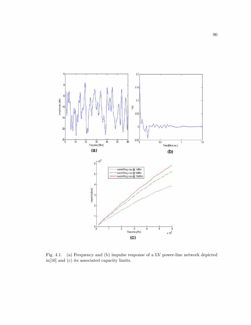
90
Fig. 4.1. (a) Frequency and (b) impulse response of a LV power-line network depictedin[10] and (c) its associated capacity limits.

91
4.3 Impulsive Noise Model
Modeling of impulsive noise over broadband power-line channels has been a chal-
lenge for researchers since early 1980s. Several different modeling methods are available.
Zimmerman and Dostert in [77] propose one of the first modeling methods for this kind
of noise at high frequencies. In their method, they use partitioned Markov models to
characterize the nature of the impulsive noise. In this section, same as in [41], we use two
simplified Markov models to represent the burst errors caused by impulsive noise. This
model has two layers. The first layer (higher layer) describes the incidence of the burst
groups and the second layer (lower layer) articulates the single impulse within the burst
group. Our model is a realistic way of representing impulsive noise in this environment.
For higher layer, the Markov model has two states of disturbed and undisturbed.
In the disturbed state, a burst group of noises happens, while in undisturbed state there
is no impulsive noise. Within the disturbed state, we define two other Markovian states
with lower time resolution: noise and no noise.
A measurement in [23] shows that the average time of the disturbed state in the
higher level is 5ms and the average time of undisturbed state is 1 second. The expected
time of the system in disturbed state is given as
Et1,2
= t
r1.∞∑k=1
k.(1− p1,22).pk−1
1,22= t
r.
11− p1,22
(4.1)
where tr1 is the time resolution for the first layer. If one considers tr1 to be 1ms,
P1 ,22 will be equal 0.8, which makes P1 ,21 equal to 0.2. Based on the average time
of disturbed and undisturbed states, the stationary state distribution of the first layer

92
model is expressed as:
π1 =[π1,1π1,2
]= [0.995 0.005] (4.2)
Thus, the transition probability matrix for the first level is:
P1 =
0.995 0.005
0.2 0.8
(4.3)
The time resolution for the second layer is selected as tr2 = 1 microsecond. The station-
ary state probabilities in the second layer are independent random variables with equal
probabilities.
π1 =[π2,1π2,2
]= [0.5 0.5] (4.4)
We assume the average duration of the disturbed and undisturbed states are 50 mi-
croseconds. This will give the transition matrix for the lower layer as:
P2 =
0.98 0.02
0.02 0.98
(4.5)
Now that we have transition probabilities, it is interesting to investigate the behavior of
burst and impulse rates. By the parameters in P1 the burst rate is equal to 1 burst per
second.
n1 =π1,1
Et1,1∼=
1− p1,11tr1
= 1per second (4.6)

93
The impulse rate during a burst noise is also calculated by equation 4.7 as well as the
parameters in P2.
n2 =π2,1
Et2,1 +
π2,2
Et2,2
= 1tr2
(π2,1.p2,12 + π2,2.p2,21
)= 20000 per second
(4.7)
The total average impulse rate is
nB
= π1,2.n2 = 100per second (4.8)
The statistical modeling of impulsive noise has been of interest to researchers for a long
time. Middleton in [47] and [64] categorizes impulsive noise in two classes of A and
B. The noise in BPL can be considered as a class A Middleton noise. Based on this
model, the noise, impulsive plus background noise, is a sequence of i.i.d random complex
variables with the probability distribution function (PDF) of:
pZ
(z) =∞∑m=0
αm
πσ2m
exp(− z2
σ2m
) (4.9)
with
αm
= e−AAm
m !(4.10)
The variance σ2
mis defined as:
σ2
m=(σ2
g+ σ
2
i
) (mA ) + Γ1 + Γ
(4.11)

94
Γ =σ2
g
σ2i
(4.12)
where σ2
gand σ
2
iare the power of background noise and impulsive noise, respectively.
The parameter A is called the impulsive index, which is the product of average rate of
impulsive noise and mean duration of a typical impulse. With our notation, the impulsive
index, A is equal to nB× t
r2. For small A, we get highly structured impulsive noise
whereas for large values of A, the noise PDF becomes Gaussian [47]. The parameter is
called background-to-impulsive noise ratio. By combining equations 4.11 and 4.12, the
variance σ2
mcan be expressed as:
σ2
m= σ
2
g
(mA ) + ΓΓ
(4.13)
Equation 4.9 shows that the PDF of noise is a weighted sum of Gaussian PDFs with
zero mean, therefore the mean and variance of noise can be acquired by the following
equations:
µz
= Ez =∫z.P
Z(z).dz
=∞∑m=0
αm. 12πσ2
m
∫z. exp(− z
2
2σ2
m
)
= 0
(4.14)

95
σ2
z= Ez2 =
∞∑m=0
αm. 12πσ2
m
∫z2. exp(− z
2
2σ2
m
)
=∞∑m=0
αmσ2
m
= σ2
g
(1 + Γ−1
)(4.15)
4.4 Impulsive Noise Cancellation
In this section, broadband communications for indoor power-line networks with
impulsive noise using Orthogonal Frequency Division Multiplexing (OFDM) is consid-
ered. Also, we employ a new estimation technique suitable for OFDM communications
systems to detect and cancel the impulsive noise in the network.
4.4.1 Decision Directed Impulsive Noise Suppression
The basic idea of OFDM is to split a high rate data stream into a number of lower
rate streams and transmit these streams simultaneously, and in parallel over a number
of orthogonal subcarriers. The orthogonality of subcarriers guarantees that the streams
do not interfere with one another. The division of data stream to several orthogonal
sub-carriers can be implemented easily using Inverse Fast Fourier Transform (IFFT).
The match filtering of each sub-channel also is done by Fast Fourier transform (FFT).
A very general block diagram realization of an OFDM system is depicted in 4.2.
R(k) = H(k)s(k) + Z(k) 1 ≤ k ≤ N (4.16)
where H(k) is the channel transfer function at kth subchannel and Z(K) is the Fourier
transform of additive noise. The decision of the transmitted data, d(k) , is made based

96
Fig. 4.2. Markov model for burst noise: (a) Modeling burst groups (b) Modeling singleimpulses within a burst group
on R(k). The block diagram of decision directed impulsive noise suppression OFDM
receiver is depicted in Fig. 4.3. The received signal, r(k), is demodulated and then the
demodulated data, d(k) is again modulated by an OFDM modulator resulting s(k) .
Since the powerline channel is slowly varying compared to the data rate, it is valid to
assume that the receiver has an accurate estimate of the channel. By convolving s(k) by
the channel estimation, an approximation of the received signal without additive noise
is obtained. Therefore, in such a way we can achieve noise estimate n(k) = r(k)−h(k) ∗
s(k) = e(k) + n(k) . e(k) is the difference between received h(k)*s(k) and h(k)* s(k) ,
and it is due to the difference between d(k) and d(k). Because of the nature of OFDM,
any estimation error in d(k) effects all the symbols in an OFDM symbol. Therefore,
e(k) has almost the same average power as n(k) with the difference that the power of
impulses are averaged within the OFDM symbols. If n(k) is subtracted from r(k), the

97
Fig. 4.3. Decision directed impulsive noise cancellation OFDM receiver diagram
noise term in r(k), n(k), is replaced by e(k). Therefore, it is sensible to only feedback
the estimation of impulsive noises. For this reason, the M largest values of estimated
noise are fed back to the original received signal in Fig. 4.3. These M values are then
subtracted synchronously from r(k). The choice of M depends on how many impulses
appear on each feedback process and it is a vital parameter for the system to perform
optimally.
To investigate the performance of this receiver and observe the effect of M on the
system operation, we simulated an OFDM system over the LV powerline channel of Fig.
4.1. The occupied bandwidth of the system is chosen to be 60 MHz. The delay spread of
the channel is 2 microseconds. To avoid ISI and ICI, while losing less than 1 dB due to
guard interval insertion, we chose an OFDM symbol interval equal to10 times the delay
spread, which is equal to 20 microseconds. The subcarrier spacing is now inverse of
20-2=18 microseconds, providing 55 KHz. By considering 60 MHz bandwidth, at most
we can use 1100 subcarriers. We designed a system with 1024 subcarriers. For each
subchannel BPSK modulation is chosen.

98
For now, we assume a very long interleaver is deployed in the system and therefore,
Middleton noise model can be used for time representation of impulsive noise. For this
matter, we chose A = 0.01 and Γ = 0.1.
The feedback process for impulsive noise suppression happens on each OFDM
symbol, i.e. 1024 bits. Fig. 4.4 shows the error probability of the system versus M for
Fig. 4.4. Effect of M on the performance of impulse cancellation
different SNRs. As it is seen in this figure, M = 10 is the optimum value for this system
and any number more or less than this value results in a non optimal performance. It
is also important to notice that a system with a high value of M does not improve the
system performance compared to a system without feedback.
The noise model used for the system above is a Middleton noise model and as
it is seen from equation 4.9, this noise can be generated in time by a Poisson process

99
with an average arrival rate λ = A . Therefore, the probability of impulsive noise for
this noise model is 1 − e−A . With A = 0.01 , the probability of an impulse is equal
to 0.01. Thereby, the average number of impulses in an OFDM symbol is equal to
1024 × 0.01 = 10.24 . This is the reason why M = 10 is the optimum number for the
impulsive noise cancellation feedback.
We use order statistics to evaluate the performance of our impulsive noise cancel-
lation algorithm. Consider the order statistics of impulsive noise zi
as random variable
yi, which is defined as follows: For any outcome δ , z
ihas the value of z
i(δ) . We order
these outcomes and define the random variable yk
as follows
y1 (δ) =∣∣∣∣zr
1
(δ)∣∣∣∣ ≤ · · · ≤ y
k(δ) =
∣∣∣∣zrk
(δ)∣∣∣∣ ≤ · · · ≤ y
n(δ) =
∣∣∣∣zrn
(δ)∣∣∣∣ (4.17)
where f|z| (z) the distribution of |z| can be easily obtained from 4.9 as f|z| (z) = 2pz
(z)
For example, yn
is the random variable that takes the largest value among n i.i.d
impulsive noise random variable of zi, i = 1...n . With this definition, the density f
k(y)
of the kth statistic yk
is given as [7],[51]:
fk
(y) =n!
(k − 1)! (n− k)!Fk−1
|z|(y)[1− F|z| (y)
]n−k
f|z| (y) (4.18)
where F|z| (z) is the distribution of the i.i.d impulsive noise random variables zi
. Our
algorithm cancels the M largest noise values. From (4.18) we can calculate the total

100
variance of the M largest noise as
σ2
cancel=M−1∑i=0
E
(y2
n−i
)(4.19)
Therefore, σ2
zthe estimated noise variance after cancellation is approximately obtained
as
σ2
z
∼= σ2
z− σ
2
cancel(4.20)
Fig. 4.5 shows the error probability of the discussed system with M = 10 on the channel
Fig. 4.5. Performance of decision directed impulsive noise cancellation receiver withM = 10.
of Fig. 4.1 with the Middleton noise model. We have also confirmed the simulations by

101
comparing to the analytical results obtained in (4.18)-(4.20) for 5 impulsive noise cancel-
lations. Also, the performance curves for a conventional OFDM system on this channel
with and without impulsive noise are depicted. The impulsive suppression technique has
significantly improved the system performance with impulsive noise. This improvement
at an error probability of 10−4 is close to 10 dB. It is important to notice that this
system is operating very similar to the case of no impulsive noise, especially at high SNR
values. Hence, one can claim at these SNRs noise impulses are completely canceled.
4.4.2 The Iterative Impulsive Noise Cancellation Algorithm
Earlier, it was argued that the number of feedback impulses, M, is a vital para-
meter for the system to perform optimally and this number needs to be equal or close
to the number of impulses in each feedback frame. Choosing a fixed M is not advisable
for a practical system, as the number of noise bursts is different for frames at different
times. Specially, if the time-based Markov model is used, it will be seen that over a very
long time, most frames are impulse free but when a burst noise arrives, those frames
hit by the burst are highly disrupted. Therefore, an algorithm needs to be employed
to estimate the number of impulses in each frame. We propose a threshold algorithm
for approximating the number of noise impulses. If the variance of background noise is
known to the receiver, a threshold value, NT
can be set such that the probability that
absolute value of background noise becomes larger than NT
is a very small number, PT
. If the absolute value of the estimated noise is greater than NT
, the noise is considered
impulsive, otherwise it is background noise. With this algorithm, the number of feedback
impulses changes for each frame.

102
Fig. 4.6. Performance of proposed iterative algorithm in a Markov-based noise modelenvironment.

103
This algorithm can be repeated iteratively, as well. After the first iteration, the
demodulated data d(k) is more accurate than before the impulsive noise cancellation.
Therefore, this more accurate estimate of the sent signal can be used again for the
next round of noise estimation with a lower threshold level. As the number of feedback
impulses is not fixed, those impulses that were missed in the last iteration with a high
probability will be detected on this iteration. Similarly, the ones that were misinterpreted
as impulsive in the former round, with high probability will be discarded this time. The
number of necessary iterations depends on the impulsive noise characteristics.
To explore the performance of this proposed algorithm, we simulated the discussed
system on the channel of Fig. 4.9 with a Markov-based impulsive noise model. The first
layer of the noise model has P1 =
0.99 0.01
0.2 0.8
as its transition probability matrix
and the second layer’s transition probability matrix is P2 =
0.98 0.02
0.02 0.98
. This
model has the same PDF as the Middleton noise model we used before with A = 0.01
and Γ = 0.1 . We employed the earlier system designed for Middleton noise model
with M = 10 , on this channel condition and the result is illustrated in Fig. 4.6.
Performance curves of a conventional OFDM system over this channel with and without
impulsive noise are shown in Fig. 4.6 , as well. The fixed size feedback algorithm
improves the system performance slightly, although the noise model that this algorithm
was designed for has the same statistics of the noise in this environment. Furthermore,
the proposed iterative algorithm with PT
= 10−5 was deployed under the same channel
condition and its performance curves are plotted in Fig. 4.6. The first iteration has

104
improved the system considerably and the second iteration with PT
= 10−4 makes the
system operate in an almost impulsive noise free condition. More iterations improve this
system insignificantly, because the second iteration’s performance is very close to the no
impulsive noise situation and this is the limit of improvement.
4.5 Bit Loading and Power optimization
In this section, broadband communications for indoor powerline networks with
impulsive noise using Adaptive bitloading and power optimization is considered. Adap-
tive modulation and bit allocation is an important technique that yields increased data
rates over non-adaptive uncoded schemes. An inherent assumption in channel adapta-
tion is some form of channel knowledge at both the transmitter and the receiver. Given
this knowledge, both the transmitter and receiver can have an agreed upon modulation
scheme for increased performance. Bitloading has been previously considered for power-
line channel [9],[50],[55],[42],[56]. In this section optimum and suboptimum algorithms
for adaptive modulation and bit allocation are applied to OFDM communication system
and a proper mathematical description of the problem is given.
4.5.1 Adaptive OFDM algorithm for increasing data rate
The objective of this optimization is to maximize the data rate, Rb for a given total
transmission power Ptotal such that the received data achieves a specified performance.
The performance criteria are application-dependent. For hard-decision coding systems
or systems without coding probability of error is chosen criterion. As soft-decision,
minimum distance decoding is widespread in data transmission, the mean squared signal

105
separation (MSSS) is the performance criterion for such systems. For now, we assume a
general criterion, which has value ci on each subchannel and average C per bit over all
the subchannels.
The objective is to maximize data rate Rb
=N∑i=1
biby optimizing the allocation of
power, Pi, and data rates bi on each of N subchannels, such that the following constraint
is satisfied:
C =
N∑i=1
ci
Rb
= Cmax (4.21)
where the parameter ci is assumed to be zero for any subchannel on which bi= 0 .
Define b to be the vector of bi’s and P to be the vector of corresponding P
i’s.
Then, the optimization problem is stated as follows:
Maximize Rb
=N∑i=1
bi
with respect to b and P ∈ RN subject to
h1 =N∑i=1
Pi− P
total= 0 (4.22)
and
h2 = C − Cmax
= 0 (4.23)
Using the Lagrange multiplier method [48], the Lagrangian function is defined:
L(b,P , λ1, λ2) = −Rb+ λ1h1 + λ2h2 (4.24)

106
The vectors b∗ and P∗ are optimum when:
L(b∗,P∗, λ1, λ2) = −∇Rb+ λ1∇h1 + λ2∇h2 (4.25)
which results in the following two equations:
−∂Rb∂bi
∣∣∣∣b∗,P∗ + λ1
L∑j=1
∂Pj∂bi
∣∣∣∣b∗,P∗ + λ2∂C∂bi
∣∣∣∣b∗,P∗ = 0 (4.26)
−∂Rb∂Pi
∣∣∣∣b∗,P∗ + λ1
L∑j=1
∂Pj∂Pi
∣∣∣∣b∗,P∗ + λ2∂C∂Pi
∣∣∣∣b∗,P∗ = 0 (4.27)
for all i such that bi 6= 0. Since Rb is independent of power distribution and also Pi is
independent of data allocation the equations (4.26) and (4.27) give:
−1 + λ2∂C∂bi
∣∣∣∣b∗,P∗ = 0 (4.28)
λ1 + λ2∂C
∂Pi
∣∣∣∣b∗,P∗ = 0 (4.29)
Therefore, the optimum solution is found by solving the gradient conditions
∂C∂bi
∣∣∣∣b∗,P∗ = ξ1 (4.30)
∂C∂Pi
∣∣∣∣b∗,P∗ = ξ2 (4.31)

107
for all i such that bi 6= 0, where ξ1 and ξ2 are constants such that Rb
=N∑i=1
bi
,
N∑i=1
Pi
= Ptotal
and C = Cmax . The solution found is a strict global minimum if the
Hessian
∇2L(b,P, λ) = −∇2Rb + λ
T∇2h (4.32)
is positive semi-definite,i.e., the Lagrangian function is convex.
4.5.2 Error probability criterion
This criterion is considered by most researchers for adaptive loading algorithms
in OFDM systems, such as in [12]. With this criterion C is the average bit error
probability, pe. Thus, the received data must achieve a specified bit error probabil-
ity pe= pmax= Cmax . If the bit error probability on the i-th subchannel is denoted by
pi then ci , which is the symbol error probability on the i-th subchannel will be equal
to bi × pi . Based on the definition of bit error probability, the criterion C is given by
(4.33).
C = pe
=
N∑i=1
bipi
N∑i=1
bi
=
N∑i=1
ci
Rb
(4.33)
By applying (4.33) to (4.30) and (4.31) the optimum conditions become:
∂C
∂bi
∣∣∣∣∣b∗,P∗
=1Rb
N∑j=1
∂cj
∂bi
− pmax
∣∣∣∣∣∣b∗,P∗
= ξ1 (4.34)

108
∂C
∂Pi
∣∣∣∣∣b∗,P∗
=1Rb
N∑j=1
∂cj
∂bi
∣∣∣∣∣∣b∗,P∗
= ξ2 (4.35)
If we assume an ICI-free OFDM system then the symbol error on each subchannel
depends only on the bit allocation on the same subchannel. Therefore, the optimum
conditions will be:
∂ci∂bi
∣∣∣∣b∗,P∗ = ψ1 (4.36)
∂ci∂Pi
∣∣∣∣b∗,P∗ = ψ2 (4.37)
If M-ary QAM modulation is utilized for each subchannel with Mi=2 ki when ki
is even, then the symbol error probability in i-th subchannel, ci is given by:
ci= 1− (1− P
i,√M
i
)2 (4.38)
where Pi,√M
i
for a QAM modulation with N subcarrier with fading coefficient ofHk, k =
1...N is given by
Pk,√M
= 2(1− 1√M
)Q(
√√√√√ 3 H2kEav
(M − 1) σZ
) (4.39)
Now, equation (4.38) can be applied to optimum conditions of (4.36) and (4.37) to find an
optimum solution. Unfortunately, by doing so an explicit expression for biand P
icannot
be obtained, hence Rb
cannot be calculated directly [48]. However, by help of iterative
algorithm, the optimum distribution of power and bit allocations can be calculated. This
algorithm will be discussed later in this section.

109
4.5.3 MSSS criterion
MSSS is defined to be the mean squared error of the received signal divided by the
average distance of points in the signaling constellation. Suppose that on subchannel i,
adjacent points x and y in the received signal constellation at the sampled output of the
matched filter for a noise-free transmission are separated by a distance ri(x, y) = |x− y|
Over the Miconstellation points, the average of points’ distance squared is then defined
as
σ2
i= E
∣∣∣ai− a
i
∣∣∣2 (4.40)
where ai is the transmitted data symbol on subchannel i and ai
is the corresponding
received symbol. The MSSS criterion for each subchannel, ci is defined by
ci= ε
i=σ2
i
d2i
(4.41)
Therefore, the average MSS per bit criterion, C, is written as
C = ζ =
N∑i=1
σ2
i
d2
iN∑i=1
bi
=
N∑i=1
εi
Rb
(4.42)
By applying (4.42) to (4.30) and (4.31) and assuming no ICI, the optimum conditions
become:
∂ci∂bi
∣∣∣∣b∗,P∗ = ψ1 (4.43)

110
∂ci∂Pi
∣∣∣∣b∗,P∗ = ψ2 (4.44)
To utilize the optimum conditions more specifically, we choose our system to have
an M-ary QAM on each subchannel. The system is ISI and ICI free, as well. The received
signals pass through a matched filter on each subchannel. Then they multiply by a gain,
specific for each subband, to minimize the MSE between the transmitted and received
symbol. If gi is the gain on the i-th subchannel, the received symbol at this subband is
ai= H
2
igiai+H
igini
(4.45)
in which ni is the additive noise at subband i and Hi is the amplitude of transfer function
of the same subband. Hi is assumed to be constant over the band of that subchannel.
Thereby, from (4.40) the MSE between the transmitted and received symbol is equal to
σ2
i= (1− g
iH
2
i)Ei+H
2
iN0 (4.46)
where N0 is the power additive noise and is the energy of transmitted symbol on i-th
subchannel, which is equal to Pi divided by the bandwidth of subband i. The optimum
receiver gain to minimize σ2
iis equal to
gi=
Ei
N0 + EiH2i
(4.47)

111
and consequently the MSE is given by
σ2
i=
EiN0
N0 + EiH2i
(4.48)
From [53] and by considering the matched filter and gain at the receiver, the average of
points’ distance squared in a noise free transmission is equal to
d2
i=
3Ei(H2
igi)2
2(Mi− 1)
(4.49)
By combining (4.49) and (4.48) and (4.47), the expression (4.41) for ci= ε
ican be uti-
lized. Subsequently, the optimum conditions of (4.43) and (4.44) are exploited. Unfor-
tunately, similar to the other case, these equations are not explicitly solvable. However,
the iterative algorithm presented in next section can find the solution for both criteria.
4.5.4 Iterative algorithm
The optimization conditions of (4.30) and (4.31) often are not explicitly solvable
but require an iterative solution. The optimization of the transmission is performed
using a steepest descent algorithm to assign the data and power among the subchannels.
After the initialization, the optimization can be broken into two sub-problems,
i.e., minimize C with respect to: 1) the subchannel bit allocation and 2) the power
distribution. The overall data rate is increased at each step to ensure that the solution
is feasible, i.e., achieves the constraints.
112
For better understanding of the algorithm, we define for variables for each sub-
channel as follows:
∆ c+
i,b= c
i
∣∣∣b
i+∆b,P
i− c
i
∣∣∣b
i,P
i
(4.50)
∆ c−i,b
= ci
∣∣∣b
i,P
i− c
i
∣∣∣b
i−∆b,P
i
(4.51)
∆ c+
i,P= c
i
∣∣∣b
i,P
i+∆P
− ci
∣∣∣b
i,P
i
(4.52)
∆ c−i,P
= ci
∣∣∣b
i,P
i− c
i
∣∣∣b
i,P
i−∆P
(4.53)
The optimization procedure can then be described with following steps: 1) Ini-
tialization: system initialized at a condition on which constraints (4.22) and (4.23) are
satisfied
2) Minimize C with respect to bi : Select the minimum allowed increment or decre-
ment of bit allocation, ∆b. In QAM system, this parameter has to be a multiplicand of 2.
Afterward, for each subchannel calculate the terms ∆c+i,b
and ∆c−i,b
. Find subchannels
I and J such that ∆c+I,b
= min
∆c+i,b
and ∆c−
J,b= min
∆c−
i,b
where ∆c+
I,b>0 and ∆c−
J,b<0 and I J. Then, if
∣∣∣∣∆c+I,b
∣∣∣∣ <∣∣∣∣∆c−J,b
∣∣∣∣ , transferring
∆b from subchannel J to I will result in the largest decrease in C. Thereby, increase bI

113
by ∆b and decrease bJ by the same amount. Repeat this procedure with the new bit
allocation until∣∣∣∣∆c−
J,b
∣∣∣∣ ∣∣∣∣∆c+I,b
∣∣∣∣ . At this point, no further transfer will reduce C.
3) Find the highest feasible bi : At step 2 the constraint (4.23) is no longer valid.
Therefore, it is possible to increase the bit rate to meet this constraint. Find the sub-
channel I such that
∆c+I,b
= min
∆c+i,b
(4.54)
Then, if Cmax - C ∆c+I,b
, increasing the number of bits in subchannel I by ∆b will
result in th smallest increase in C. Increase bI by ∆b. Repeat this process until ∆c+I,b
>Cmax - C.
4) Minimize C with respect to Pi : Select the minimum allowed increment or
decrement of power distribution, ∆P . Afterward, for each subchannel calculate the
terms ∆c+i,P
and ∆c−i,P
. Find subchannels I and J such that ∆c+I,P
= min
∆c+i,P
and ∆c−
J,P= min
∆c−
i,P
where ∆c+
I,P<0 and ∆c−
J,P>0 and I < J . Then, if
∣∣∣∣∆c+I,P
∣∣∣∣ >∣∣∣∣∆c−J,p
∣∣∣∣ , transfer-
ring ∆P from subchannel J to I will result in the largest decrease in C. Thereby, increase
PI by ∆P and decrease PJ by the same amount. Repeat this procedure with the new
bit allocation until∣∣∣∣∆c+
I,P
∣∣∣∣ ∣∣∣∣∆c−J,P
∣∣∣∣ . At this point, no further transfer will reduce C.
5) Repeat step 3.
Steps 2 and 3 are considered as bit loading process and steps 4 and 5 as power load-
ing. Both bit loading and power loading algorithms are suboptimum subroutines. Based
on application and considering the complexity of the system, each of these suboptimum
routines can be selected instead of the entire complex optimum algorithm. We applied
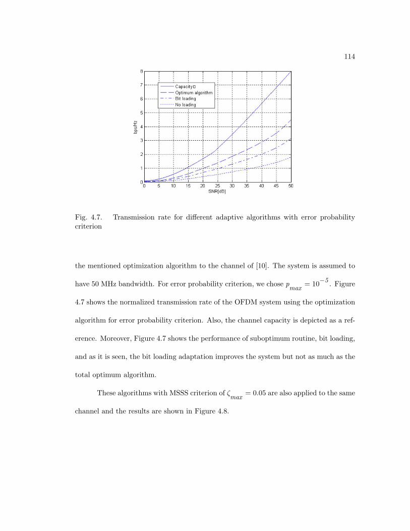
114
Fig. 4.7. Transmission rate for different adaptive algorithms with error probabilitycriterion
the mentioned optimization algorithm to the channel of [10]. The system is assumed to
have 50 MHz bandwidth. For error probability criterion, we chose pmax = 10−5 . Figure
4.7 shows the normalized transmission rate of the OFDM system using the optimization
algorithm for error probability criterion. Also, the channel capacity is depicted as a ref-
erence. Moreover, Figure 4.7 shows the performance of suboptimum routine, bit loading,
and as it is seen, the bit loading adaptation improves the system but not as much as the
total optimum algorithm.
These algorithms with MSSS criterion of ζmax = 0.05 are also applied to the same
channel and the results are shown in Figure 4.8.

115
4.5.5 Adaptive OFDM algorithm for improving system performance
The objective this optimization is to maximize the system performance for a given
total transmission power Ptotal such that the received data is transmitted by a certain
bit rate Rbmax
=N∑i=1
bi
. Similar to the last situation the performance criterion is
application-dependent and can be either error probability or MSSS.
Fig. 4.8. Transmission rate for different adaptive algorithms with MSSS probabilitycriterion.
We can state the optimization problem as bellow:
Maximize C =
N∑i=1
ci
Rb
with respect to b and P ∈ RN

116
Fig. 4.9. The effect of adaptive OFDM loading to the performance of a communicationsystem

117
Subject to h1 =N∑i=1
Pi− P
total= 0 and h2 = Rb−Rbmax=0 Following the steps
mentioned in the last section, we can express the optimization conditions as:
−∂C∂bi
∣∣∣∣b∗,P∗ + λ2 = 0 (4.55)
−∂C∂bi
∣∣∣∣b∗,P∗ + λ1 = 0 (4.56)
Similar to the last case, the optimization conditions cannot be explicitly solved for any of
MSSS and error probability criteria. Therefore, the iterative steepest descent algorithm
needs to be applied. For this case, the optimization procedure follows steps 1,2 and 4
of introduced algorithm in the last section because the data rate is fixed and therefore
steps 3 and 5, which adapt the data rate are redundant. Likewise, suboptimum routines
of bit loading and power loading are also applicable in this situation.
These optimum and suboptimum algorithms are applied to an OFDM communi-
cation system and the results are illustrated in Figure 4.9 . The original system uses a
QPSK scheme for all the subchannels with overall data rate of 90Mbits/sec. As it is seen,
bit loading shows better improvement than power loading in this system. The optimum
adaptive algorithm improves the system performance by 6dB at an error probability of
10−6.

118
4.6 Performance Analysis of Coded MC-CDMA in Powerline Commu-
nication Channel with Impulsive Noise
In this section Broadband communications for indoor power-line networks with
impulsive noise using Multicarrier CDMA (MC-CDMA) is considered. The bit error rate
(BER) performance of the MC-CDMA system under impulsive noise and frequency fad-
ing is theoretically analyzed and closed form expression for this performance is derived.
Furthermore, a theoretical upper bound for performance of coded MC-CDMA system is
derived, given perfect interleaving and effect of interleaver length on coding performance
is also studied. Simulations show that the upper bound is quite tight for the case of
employing a longer interleaver.
4.6.1 Multicarrier System
In this section we describe the MC-CDMA system model. We assume that all the
users experience the same channel multipath and also they are synchronous. While these
assumptions may not be realistic in the context of a wireless fading channel with many
users and fast channel variations, for an indoor LV network with typically limited number
of users and fixed channel our assumptions are reasonable. We consider a downlink MC-
CDMA system with K users employing binary phase-shift keying (BPSK) and binary
spreading sequences. Input data from each user is first converted to P parallel stream
and each bit is spread over L spreading chips. Therefore, the transmitted signal for user

119
k is given as,
sk(t) =
+∞∑n=−∞
√2E
bLT
s
P∑p=1
L∑l=1
dk,p
(n)ck,luTs
(t− nTs)
cos(wp+(l−1)P t+ φ
p+(l−1)P )
(4.57)
where Eb
and Ts
are the bit energy and bit (or chip) duration respectively, uTs
(.) is the
rectangular waveform of duration Ts. ck,l
is the lth chip of the user k, dk,p
(n) is the nth
data bit in the pth data stream of user k, wi= 2πf
iis the ith carrier frequency and φ
i
is the phase of the ith carrier. In practice, the multicarrier modulation is implemented
by inverse fast Fourier transform (IFFT). We mention the procedure to consider the
effect of impulsive noise. When the transmitted signal is an OFDM symbol, the received
symbol after front-end filtering and sampling is given by:
ri=
1√M
M−1∑m=0
ame
j2πmiM
⊗ hi+ z
i, i = 0, . . . ,M − 1 (4.58)
where am
is a data symbol taking the spread code bits values, hi
is the discrete channel
impulse response and M is total number of carrier used which is equal to LP . Note
that, just one user is considered since we want to calculate the effect of impulsive noise
at the receiver. The receiver performs an M point discrete Fourier transform (FFT), as
follows:
Rm
=1√M
M−1∑i=0
rie
j2πmiM = a
mHm
+Gm,m = 0, . . . ,M − 1 (4.59)

120
where Gm
is the DFT of zi, expressed as:
Gm
=1√M
M−1∑i=0
zie
j2πmiM ,m = 0, . . . ,M − 1 (4.60)
As mentioned earlier, the zi
are i.i.d random variables with a distribution function as
in eq. (4.9). According to Central Limit Theorem, if a sample mean x is obtained from
samples that are taken from a large population, and the samples are of a sufficiently large
ensemble size, the distribution of x is well approximated by a Gaussian distribution.
This Gaussian distribution is characterized by a mean µx
= µ and a standard deviation
σx
= σ/√k , where µ and σ are the mean and standard deviation of the population and
K is the sample size. By considering eq. (4.60), we can express Gm
as:
Gm
=√M
1M
M−1∑i=0
z′m
(4.61)
in which
z′i= z
ie− j2πim
M (4.62)
Therefore, based on Central Limit Theorem, Gm
is Gaussian with a mean µg
=
µz′ = 0 and a standard deviation σ
g=√M.(σ
z′/√M) = σ
z, in which σ
zis expressed by
(4.15). DFT procedure spreads the effect of impulsive noise over multiple subcarriers in
a way that noise on each subband exhibits a Gaussian behavior. This is one of the major
benefits of OFDM system in presence of impulsive noise [44]. Therefore the received

121
MC-CDMA symbol is expressed as
r(t) =+∞∑
n=−∞
√2E
bLT
s
K∑k=1
P∑p=1
L∑l=1
Hk,p+(l−1)P dk,p(n)c
k,l
uTs
(t− nTs)cos(w
p+(l−1)P t+ φp+(l−1)P ) + ν(t)
(4.63)
where ν(t) is the effective noise in the receiver after DFT which comes from AWGN and
impulsive noise as described earlier and hk,i
is the fading amplitude for the kth user and
ith subcarrier. For downlink channel we have hk,i
= hi. Considering the decision metric
in the pth stream of the first user, without loss of generality, we obtain
Up
=Ts∫
0r(t)
L∑l=1
c1,lcos(wst+ φs)g1,sdt
= Dp
+ I + ν
(4.64)
where s = p+(l−1)P , g1,s is the first user’s combining coefficients for the sth subcarrier
and Dp
is the desired signal which is obtained as
Dp
=
√EbTs
2L
L∑l=1
hsg1,s. (4.65)
The noise ν has a zero mean and a variance of
σ2Ts
4
L∑l=1
g2
s(4.66)

122
and I represents the multiuser interference
I =
√EbTs
2L
K∑k=1
dk,p
L∑l=1
ck,lc1,lhsgs (4.67)
There are several schemes for combining the chips of the same data bit; equal gain
combining (EGC), maximum ratio combining and Orthogonality restoring Combining
(ORC). Using ORC, which outperforms the other schemes under high load condition at
high SNR values [22], the orthogonality among different subcarriers is restored . For
ORC the combining coefficients are
gs
=1hs
(4.68)
Using Walsh-Hadamard spreading codes, which have zero correlation, the multiuser in-
terference term equals zero. Therefore, the BER for the pth stream is obtained as
Pep
= Q(
√√√√√√2LE
b
σ2 L∑l=1
h−2s
) (4.69)
Assuming a uniform bit allocation probability for different streams, the average BER of
the system is obtained as:
Pe =1P
P∑p=1
Pep. (4.70)

123
4.6.2 Coded MC-CDMA system Analysis
The Pair-wise Error Probability (PEP) represents the probability of choosing
the coded sequence X =(x1, x2, ..., xL
)when indeed another code sequence X =(
x1, x2, ..., xL
)was transmitted, where L is the frame length. Under the assumption of
perfect channel state information (CSI), the conditional PEP with respect to the channel
coefficients h =(h1, h2, ..., hN
)is expressed as
P(X, X|h
k
)= Q
√√√√√ε
(X, X
)2N0
(4.71)
where ε(X, X
)is the energy difference between two codewords. With the assumption
of BPSK we have,
P(X, X
∣∣∣hk
)= Q
√√√√2Es
N0
∣∣∣Ωk
∣∣∣ (4.72)
where Es
is the total transmitted energy and Ωk
is the set of bit interval locations where
X and X differ in the kth subchannel and where |Ω| is the cardinality of Ω, which also
corresponds to the length of the error event. Defining the signal-to-noise ratio as τ =
Es
/N0 and using the upper bound on Gaussian-Q function, i.e. Q (
√z) ≤ 0.5 exp (−z/2)
under the assumption of symbol-by-symbol interleaving, we obtain
P(X, X
∣∣∣hk
)≤ 1
2[exp (−τ)]
∣∣∣Ωk
∣∣∣(4.73)

124
PEP is the basic tool for the derivation of union bounds on the error rate perfor-
mance of a coded communication system. A union bound on the average BER on the
kth subchannel can be found as in [53]:
Pbk
≤∑X
P (X)∑X 6=X
q(X, X
)P(X, X|h
k
)(4.74)
where P (X) is the probability that the sequence X is transmitted, q(X, X
)is the
number of information bit errors in choosing another coded sequence X instead of X.
For uniform error probability codes, a symmetry property exists, eliminating the need
for averaging over all possible transmitted sequences, which leads to
Pbk
≤∑X 6=X
q(X, X
)P(X, X|h
k
)(4.75)
In the case that PEP is expressed as in a product form, the transfer function
technique [53] provides an efficient method for the computation of (4.75), i.e.,
Pbk
≤ ∂
∂sT(Dk, s)∣∣∣∣s=1
(4.76)
As an example, we consider a convolutionally coded system to demonstrate BER
results. The code has a rate of 1/2 and a constraint length of 3. The transfer function
of this code is found to be
T (D, s) =D
5s
(1− 2sD)(4.77)

125
Since the code satisfies the uniform error property, we can use eq. (4.76) for BER
performance evaluation and after averaging over subchannels, the BER performance is
obtained as
Pb≤ 1N
N∑k=1
D5k(
1− 2Dk
)2 (4.78)
4.6.3 Simulation and Analytical Results
For our analysis and simulation purposes, we designed an MC-CDMA system for
the channel introduced. The occupied bandwidth of the system is chosen to be 60 MHz.
The capacity limit of this channel at 60 MHz with 10-dBm launched power is around
600 Mbits/sec. The delay spread of the channel is 2 microseconds. To avoid ISI and
ICI, while losing less than a 1 dB due to guard interval insertion, we choose an OFDM
symbol interval equal to10 times the delay spread, which is equal to 20 microseconds.
The subcarrier spacing is now the inverse of 20-2=18 microseconds, providing 55 KHz.
By considering 60 MHz bandwidth, at most we can use 1100 subcarriers. We designed
a system with 1024 subcarriers and one known pilot channel for estimation. For the
MC-CDMA system, we have picked L = 8 and P = 256 and the spreading code is
Walsh-Hadamard. Fig. 4.10 shows the performance of such a system without coding,
analytically and by computer simulations. For simulation results, two noise models
were considered: the time-Markov model and the statistical model of eq. (4.9). Both
models are utilized by the parameters described in section 4.2. As a side result in
this section, it is shown that results by both these models are in agreement. One should
notice that Markov based model is a time representation of the noise, whereas Middleton
model is a statistical illustration which is generated i.i.d in time, therefore the statistical

126
characteristics of the time domain model over a long time will be the same as Middleton’s
expression. Our simulations using Markov model are run for a long period of time.
Consequently, as it is confirmed in Fig. 4.10 , both models results show an exact match.
Fig. 4.10. Uncoded MC-CDMA system over impulsive noise frequency selective channel,simulation and analytical comparisons
As mentioned before, bursty errors deteriorate the performance of the coding
scheme used in any communications system. Burst errors can happen either by im-
pulsive noise or by deep frequency fades. Powerline channels suffer from both of these
deficiencies; therefore a mechanism is needed to disperse the error bursts both in time
and frequency. For this purpose, interleavers have been utilized since early days of digital
communications. Due to the delay introduced by an interleaver, the length of interleavers

127
is always an issue of concern for systems practical implementations, thus several studies
have been conducted throughout research history in order to find an efficient and low
complexity interleaving method. MC-CDMA system has an inherent property that it
disperses impulsive noise bursts by N symbols (N is the number of carriers) thanks to
the FFT in the implementation of the demodulator at the receiver. However, by using
a time interleaver this property is destroyed. Thereby, in multicarrier systems shuffling
bits in time and frequency is desired. In doing so, we adopted the method introduced
by Ramseier in [54] for our designed system. This method has a very easy to imple-
ment ”diagonal” strategy. The interleaver size has two constraints on length and depth.
The length parameter accounts for reordering the bits in one OFDM symbol and it is
responsible to disperse the affected bits by channel fadings. The depth factor justifies
shuffling the bits over several OFDM symbols in time and it takes care of separating the
distorted symbols by impulsive noise. For our simulations, we considered three different
interleavers: one interleaver with size 1024 × 16, which shuffles bits of sixteen OFDM
symbols and two other interleavers with sizes of 1024× 128 and 1024× 1024. Fig. 4.11
shows the performance results of the coded MC-CDMA system with impulsive noise in
the LV-PLC channel medium for different interleaver sizes. The simulation results clearly
show that increasing the size of the interleaver improves the performance. Specifically,
increasing the interleaver depth from 16 to 128 yields more than 1dB gain in SNR at a
BER of 10−6. However, further increasing the interleaver depth from 128 to 1024 gives
about 0.5dB gain. Fig. 4.11 also shows the calculated upper bound in 4.75. As it can
be realized, the upper bound is close to the curve of interleaver size of 1024 × 1024 for
high SNR values, since it is calculated under the assumption of ideal (infinite) interleaver

128
Fig. 4.11. Coded MC-CDMA simulation results and analytical upper bound assuminginfinite interleaver
size. This fact shows that increasing the interleaver size more than 1024× 1024 will not
improve the performance of the system.
4.7 Conclusions
In this chapter, we investigated communications system performance for an indoor
power-line channel with bursty impulsive noise. First we introduced the LV powerline
channel model and also impulsive noise model.
In section 3, we evaluated the performance of a decision-directed impulsive noise
cancellation algorithm (which was introduced earlier in [17] for ultra wideband communi-
cations) under powerline channel conditions. We discussed that the number of feedback
impulsive noise is a vital parameter for this system to perform optimally and it is needed
to change this number by each feedback according to the number of impulses. Moreover,

129
we proposed an algorithm that estimates the number of impulses. This algorithm can be
applied iteratively, to find better estimates of the impulsive noise. Simulations showed
that under a practical and realistic condition of impulsive noise channel, our proposed
iterative algorithm outperforms the fixed size feedback algorithm, significantly. With
this method, after a very few iterations, most of the noise impulses are detected and
canceled.
In section 4, we analyzed the performance of a multicarrier modulation communi-
cations system performance with adaptive loading optimization in a power-line channel
medium. OFDM can make a very efficient use of allocated bandwidth and energy. How-
ever, not all OFDM subchannels experience the same channel deterioration. For this
reason, it is admissible to use more cautious communication techniques on these subcar-
riers. In this section, we examined the effect of energy and bandwidth allocation on the
system performance and we provided the optimum algorithm to achieve the desired cri-
teria. By this method, it is possible to achieve higher data rates and better performance
for an OFDM system. However, the complexity of the system is increased and transmit-
ter needs to know the channel state information. This is a reasonable assumption in a
LV powerline channel since it changes very slowly comparing to the bit rate.
In section 5, we derived the performance expression for an uncoded MC-CDMA
system under impulsive noise and highly frequency selective powerline channel medium.
Our simulations show that the closed form expression and simulation results are in
agreement. Furthermore, we deployed two noise models for impulsive noise environment,
statistical and time domain models, and computer simulations confirmed the fact that
both models represent the same environment with the same results. Additionally, the

130
upper bound for a coded MC-CDMA system was calculated, given independency of
consecutive symbols provided by perfect interleaving. Our simulations revealed that the
derived upper bound is quite tight for the case of employing a longer interleaver. It was
also shown that interleaver depth is of importance due to impulsive noise but increasing
this parameter to 1024 yields the best possible performance, i.e., perfect interleaving.

131
Chapter 5
Conclusions and Future Work
5.1 Conclusions
In this thesis, we described several communication systems scenarios and de-
scribed the channel models, where we analyzed BER or FER and tried to improve the
performance. As mentioned earlier the main focus in this work is to improve the perfor-
mance of these systems by applying channel coding techniques.
In a wireless optical communication system, optical transceivers communicate di-
rectly through the air to form point-to-point line-of-sight links. A major impairment
over wireless optical links is the atmospheric turbulence. In chapter 2, we considered
multirate fractal modulation over wireless optical links to improve the error rate perfor-
mance. The multirate scenario is a novel approach which is seriously considered as an
option to make available broadband access to the planes and satellites. We considered
Digital Fountain Codes which are a new class of erasure correction codes. Fountain codes
can produce an unlimited flow of encoding data blocks, i.e., they are rate-less.
Another problem with an optical wireless system is transmit power restriction due
to eye-safety issues. To address this problem, Multiple-Input Multiple-Output (MIMO)
systems are considered, where a diversity gain is expected at the price of higher hardware
complexity. We will show how much gain can be obtained by using MIMO system and
the effect of correlation in the transmitter lasers or the receiver photo-detectors and also

132
comparison between optimal and equal gain receivers, which overall lead to important
and interesting conclusions.
In the next part of the thesis, we considered the low voltage (LV) power-line
channel model and capacity characteristics. We described channel and noise models.
One of the major problems in PLC is multipath fading. The well-known multi-carrier
technique, Orthogonal Frequency Division Multiplexing (OFDM) used as the modulation
scheme to address this problem. By the application of OFDM, the most distinct property
of powerline channel, its frequency selectivity due to multipath, can be easily coped with.
On the other hand, Code Division Multiple-Access (CDMA) is an attractive scheme due
to robustness to interferences, which is very important in PBL communications since
there are two sources of interference, the interference from other wireless devices and
the multiuser interference in a home-network. A combination of multicarrier modulation
and CDMA, MC-CDMA, which has the advantages of both techniques, was considered.
Like other communication systems, coding was shown to improve the multicarrier system
performance but because of the nature of this channel, the achieved improvements are
usually very restricted.
Another major problem in PLC is man-made impulsive bursty noise. The im-
pulsive noise characteristics and model was discussed and an appropriate realistic model
is chosen, as well. We explained two approaches for modeling the impulsive noise, one
based on Markov model and the other based on a statistical model. We also suggested
different approaches to alleviate the effect of impulsive noise. The first scheme was based
on an iterative impulsive noise cancellation which is based on the assumption that the
channel impulse response is available in the receiver. This assumption is reasonable for

133
PLC, which changes very slowly comparing to the transmission rate. Concatenated cod-
ing was another considered approach to address impulsive noise. In this scheme, an inner
convolutional code, corrects the error due to the additive white Gaussian noise (AWGN)
and the outer code takes care of the blocks of data that are corrupted by impulsive noise
to the extent that they are not recoverable by the inner code.
5.2 Future Work
We considered a concatenated coding structure for the multirate communication
system in 2.2. In this structure the channel seen by the outer code, is effectively a binary
erasure channel (BEC), where the symbols are basically either correct or discarded.
However, as discussed earlier, the optimality of this scheme for multirate scheme is
not really dependent on the concatenated structure of the code. Therefore, another
interesting option would be using the outer code alone. In this case, we need a decoding
scheme which works for AWGN channel. Very recently, a decoding scheme for arbitrary
symmetric channels has been proposed in [18]. The most powerful efficient decoding
algorithm for this class of codes is the iterative belief-propagation (BP) algorithm. At
each iteration, this algorithm updates the probability that a given variable node is 0 or
1, given all the observations obtained in previous rounds, which is called log-likelihood
ratio (LLR) and defined as
LLR(X) = logP (X = 0|Y )P (X = 1|Y )
(5.1)

134
Therefore, the inner convolutional code is removed and more Fountain code symbols are
transmitted. We conjecture that the performance of overall scheme is improved in equal
condition of rate and interleaver size.
Part of our multirate application scheme is intended to be used for image and
video transmission. There has been some works considering joint source-channel coding
using Raptor codes. Therefore, it is possible to consider this approach in the multirate
scheme. Also, we believe that there is possibility of some interesting work for video
transmission protocols like Digital Video Broadcasting - Handheld (DVB-H) standard
in this context. Raptor codes have been proposed as FEC for application layer part
of the DVB-H standard [67]. One important requirement in video transmission is the
continuous follow of the stream even at the expense of the quality. There are several
approaches to achieve this. In Mediaflo [71], which is standard proposed by Qualcomm
for video transmission, this is done by dividing the symbol to least and most significant
digits. The least significant digits correspond to higher resolution in video quality and are
near each other in the transmitted constellation. Therefore they are not recoverable in the
low SNR values. But the important part of the constellation which corresponds to the low
resolution image are placed far from each other in the constellation and are recoverable
even in lower SNRs. There are also other approaches like Multiple Descriptions coding
[20], in which an image is decoded into multiple descriptions and each of this descriptions
increases the resolution upon reception in the receiver side. Consider the general trend
of cross-layer optimization in the protocol stacks for wireless applications, we think t
Raptor code can be used with the Mediaflo approach or MDC and come up with a
efficient source-channel coding scheme for DVB-H.

135
We have explored a number of problems in PLC and made some suggestions to
improve performance. Specially, we considered impulsive noise and using channel coding
and impulsive noise cancellation for improving performance of the system which is based
on the OFDM. One of the practical problems with using an OFDM system is the syn-
chronization between transmitter and receiver. Synchronization is needed both in time
and frequency. Frequency synchronization is mainly due to the carrier frequency offset
(CFO) of between the transmitter and receiver oscillators. The maximum likelihood
algorithm for CFO compensation is the AWGN has been derived in [13], which uses the
presence of cyclic prefix in the OFDM symbol. However, this derivation is not optimum
for the case of impulsive noise. Another interesting future work can be consideration
of derivation of ML detection criteria for CFO estimation in the presence of impulsive
noise. This is certainly a nice theoretical problem to be solved.

136
Appendix A
Lognormal Approximation
This appendix provides an approximation for the summation of correlated log-
normal random variables. Specifically, we want to approximate∑K
k=1exp
(xk
)with
a single lognormal random variable ez . Defining cov
(xk, xl
)= v
kl, v
kk= σ
2
x,
E(xk
)= −σ2
x
/2 and using the results reported in [60] and [11], we have
µz
= log
α√1 + β2
α2
(A.1)
σ2
z= log
(1 +
α2
β2
)= log
1 +1
K2
∑k,l
evkl − 1
(A.2)
Here, α and β are defined as
α = K (A.3)
β2 =
K∑k=1
K∑l=1
(evkl − 1) (A.4)
respectively. Under the assumption of weak turbulence, i.e. vkk
<< 1 , and small
correlation values, i.e. vkl<< 1 , (A.1) and (A.2) reduce to
µz∼= logK −
σ2
z2
(A.5)

137
σ2
z≈ 1
K2
∑k,l
evkl − 1
≈ 1Kv11 +
1
K2
∑k 6=l
vkl
(A.6)
where we assume that lognormal variance is equal for all channels, i.e., vkk
= v11 = σ2
x.

138
Appendix B
List of Publications
Journals
(1) S. M. Navidpour and M. Uysal, M. Kavehrad ”Performance Bounds for Coded Free-
Space Optical Communications under Correlated Gamma-Gamma Atmospheric Turbu-
lence Channels”, Submitted to Journal of Optical Networking.
(2) S. M. Navidpour and M. Uysal, M. Kavehrad ”BER Performance of MIMO Free-
Space Optical Links”, Submitted to IEEE Tran. Wireless Commun., Feb. 11, 2006.
(3) M. Uysal, S. M. Navidpour and J. Li,”Error Performance of Coded Free-Space Op-
tical Links over Strong Turbulence Channels”, IEEE Communication Letters, Oct 2004.
(4) P. Amirshahi, S.M.Navidpour and M.Kavehrad, ”Performance Analysis of Uncoded
and Coded OFDM Broadband Transmission Over Low Voltage Powerline Channels with
Impulsive Noise”, Accepted for publication in IEEE Trans. on Power Delivery.
Conferences
(1) S. M. Navidpour and M. Uysal, M. Kavehrad, ”Capacity of MIMO optical link”, To
appear in SPIE Photonic West, San Diego, 13-17 Aug. 2006.
(2) P. Amirshahi, S.M.Navidpour and M.Kavehrad, Performance Analysis of OFDM
Broadband Communications System Over Low Voltage Powerline with Impulsive Noise,
IEEE ICC’06 Conference, June 2006.
(3) S. M. Navidpour and M. Uysal, M. Kavehrad Performance Bounds for Correlated

139
Turbulent Free-Space Optical Channels, IEEE WCNC conference,Las Vegas, April 2006.
(4) P. Amirshahi, S.M.Navidpour and M.Kavehrad, Fountain Codes For Impulsive Noise
Correction In Low Voltage Indoor Powerline Broadband Communications, IEEE CCNC’06
Conference, Las Vegas, January 2006.
(5) S.M.Navidpour, P. Amirshahi and M.Kavehrad, ”An Iterative Impulsive Noise Can-
cellation Technique for Multicarrier Communications Systems over Powerline Channels”,
Submitted to IEEE Globecomm’6 Conference.
(6) P. Amirshahi, S.M.Navidpour and M.Kavehrad,”Bit loading and power optimization
for powerline communication channel”, Submitted to IEEE Globecomm’6 Conference.
(7) S.M.Navidpour, B.Hamzeh and M.Kavehrad, Multirate Fractal Free Space Optical
Communications using Fountain Codes, SPIE- photonics East, Boston, Oct 2005.
(8) S. M. Navidpour and M. Uysal, ”Analysis of Coded Optical Wireless Communication
under Correlated Gamma-Gamma Channels”, IEEE VTC04-Fall, Los Angeles, Califor-
nia, USA, September 2004.
(9) S. M. Navidpour and M. Uysal, ”BER Performance of MIMO Free-Space Optical
Links”, IEEE VTC04-Fall, Los Angeles, California, USA, September 2004.
(10) S.M.Navidpour, P. Amirshahi and M.Kavehrad, ”Performance Analysis of Coded
MC-CDMA in Powerline Communication Channel with Implusive Noise”,IEEE ISPLC’06
Conference, Orlando,March 2006.

140
References
[1] R. Nabar A. Paulraj and D. Gore. Introduction to Space-Time Wireless Communi-
cations. Cambridge University Press, 2003.
[2] A. Abdi and M. Kaveh. K distribution: An appropriate substitute for rayleigh-
lognormal distribution in fading-shadowing wireless channels. IEE Electronics Let-
ters,, 34:851–852, April 1998.
[3] A. Abdi and M. Kaveh. Comparison of dpsk and msk bit error rates for k and
rayleigh-lognormal fading distributions. IEEE Communication Letters,, 4, April
2000.
[4] P. Amirshahi and M. Kavehrad. Transmission channel model and capacity of
overhead multi-conductor medium-voltage power-lines for broadband communica-
tions. In IEEE Consumer Communications and Networking Conference, Las Vegas,
Nevada, 2005.
[5] S. Arnon. Effects of atmospheric turbulence and building sway on optical wireless
communication systems. Optics Letters, 28, Jan. 2003.
[6] S. Arnon. Optimization of urban optical wireless communication systems. IEEE
Transactions on Wireless Communications, 2, July 2003.
[7] N. Balakrishnan B. C. Arnold and H. N. Nagaraja. A First Course in Order Sta-
tistics. Wiley, New York, 1999.

141
[8] E. Woddbridge B. R. Strickland, M. J.Lavan and V. Chan. Effects of fog on the bit-
error rate of a free-space laser communication system. Applied Optics, 38, January
1999.
[9] S. Baig and N.D. Gohar. Discrete multi-tone (dmt) transceiver with dynamic rate
adaptive water-filling bit-loading technique for in-home power line communication
networks. In Multi Topic Conference. INMIC 2003. 7th International, Dec 2003.
[10] T. Banwell and S. Galli. A novel approach to the modeling of the indoor power
line channel – part i: Circuit analysis and companion model. IEEE Transactions
on Power Delivery,, 20:655–663, April 2005.
[11] N. C. Beaulieu and Q. Xie. Minimax approximation to lognormal sum distributions.
IEEE Veh. Technol., 53:479–489, March 2004.
[12] J.A.C. Bingham. Multicarrier modulation for data transmission: An idea whose
time has come. IEEE communications Magazine, May 1997.
[13] Biao Chen. Maximum likelihood estimation of ofdm carrier frequency offset. Signal
Processing Letters, IEEE, 9:123 – 126, April 2002.
[14] Thomas M. Cover and Joy A. Thomas. Elements of Information Theory. John
Wiley & Sons, Inc., N. Y., 1991.
[15] Huaiyu Dai and H.V. Poor. Advanced signal processing for power line communica-
tions. IEEE Commun. Magazine, 41, May 2003.

142
[16] C. C. Davis and I. Smolyaninov. The effect of atmospheric turbulence on bit-
error-rate in an on-off keyed optical wireless system. In SPIE Free-Space Laser
Communication Communication and Laser Imaging, 1997.
[17] Y. Dhibi and T. Kaiser. Iterative impulsive noise suppression in mixed impulse
radio and uwb-ofdm systems. In international workshop of Networking with UWB,
January 2006.
[18] O. Etesami and A. Shokrollahi. Raptor codes on binary memoryless symmetric
channels. Information Theory, IEEE Transactions on, 52:2033 – 2051, May 2006.
[19] S. Galli and T. Banwell. A novel approach to the modeling of the indoor power line
channel – part ii: Transfer function and its properties. accepted for publishing in
the IEEE Transactions on Power Delivery,, 2005.
[20] V.K. Goyal. Multiple description coding: compression meets the network. Signal
Processing Letters, IEEE, 18:74 – 93, Sept. 2001.
[21] I. S. Gradshteyn and I. M. Ryzhik. Table of Integrals, Series and Products. Academic
Press, 1994.
[22] Yong Liang Guan and Keli Zhangr. A low-complexity enhancement to multicarrier
cdma system with orc. In Proc. of ICCCAS’04, June 2004.
[23] Y.L. Guan H. Meng and S. Chen. Modeling and analysis of noise effects on broad-
band power-line communications. IEEE Transactions on Power Delivery,, 20:630 –
637, April 2005.

143
[24] S. M. Haas and J.H. Shapiro. Capacity of wireless optical communications. IEEE
Journal on Selected Areas in Communications, 21(8), 2003.
[25] Shane M. Haas, Jeffrey H. Shapiro, and Vahid Tarokh. Space-time codes for wire-
less optical communications. EURASIP J. Appl. Signal. Process., 2002(3):211–220,
2002.
[26] http://www.wcai.com/.
[27] P. Adhikari E. J. Korevaar I. Kim, H. Hakakha. Scintillation reduction using mul-
tiple transmitters. In SPIE, 1997.
[28] Huy-Myoung Oh Won-Tae Lee Kwan-Ho Kim Jae-Jo Lee, Seung-Ji Choi and Dae-
Young Lee. Measurements of the communications environment in medium voltage
power distribution lines for wide-band power line communications. In Proc. of Int’l
Symposium on Power-line Communications and its Applications, 2004.
[29] E. Jakeman and P. N. Pusey. A model for non-rayleigh sea echo. IEEE Transactions
on Antennas and Propagation,, 24(6):806–814, November 1976.
[30] E. Jakeman and P. N. Pusey. The significance of k-distributions in scattering ex-
periments. Physical Review Letters,, 40(9):546–550, Feb. 1978.
[31] E. Jakeman and P. N. Pusey. On the statistics of k-distributed noise. Journal of
Physics A,, 13:31–48, 1980.

144
[32] M.Luby J.W.Byers and M. Mitzenmacher. A digital fountain approach to asyn-
chronous reliable multicast. IEEE Journal on Selected Areas in Communications,
8:1528 – 1540, Oct. 2002.
[33] J.W.Goodman. Statistical Optics. John Wiley and Sons, 1985.
[34] G. Kaiser. A friendly Guide to Wavelets. Mass: Brickhauser, Boston, 1993.
[35] M. Kavehrad and B. Hamzeh. Laser Communication System Using Wavelet-Based
Multi-Rate Signaling. In Proceedings of IEEE MILCOM, Monterey-California, No-
vember 2004.
[36] D. Kedar and S. Arnon. Urban optical wireless communication networks: The main
challenges and possible solutions. IEEE Communication Magazine, 42, May 2004.
[37] R. L. Phillips L. Andrews and C. Y. Hopen. Laser Beam Scintillation with Appli-
cations. SPIE Press, 2001.
[38] C. Y. Hopen L. C. Andrews, R. L. Phillips and M. A. Al-Habash. Theory of optical
scintillation. Journal of Optical Society America A, 16(6):1417–1429, June 1999.
[39] Fredrik Ljungberg, Per Dahlberg, and Johan Sanneblad. Supporting opportunistic
communication in mobile setting. In ACM Conference on Human Factors in Com-
puting Systems (CHI’2000), pages 111–112, The Hague, The Netherlands, April 1–6
2000.
[40] P. Lombardo and A. Farina. Coherent radar detection against k-distributed clutter
with partially correlated texture. Signal Processing (Elsevier), 48:1–15, 1996.

145
[41] K. Dostert M. Babic, M. Hagenau and J. Bausch. Theoretical postulation of plc.
In IST integrated project No. 507667.
[42] J.Y. Baudais M. Crussiere and J.F. Helard. Robust and high-bit rate communi-
cations over plc channels: a bit-loading multi-carrier spread-spectrum solution. In
Power Line Communications and Its Applications, 2005 International Symposium
on, April 2005.
[43] S. M. Navidpour M. Uysal and J. Li. Error rate performance of coded free-space opti-
cal links over strong turbulence channels. IEEE Communications Letters, 8(10):635–
637, Oct. 2004.
[44] Y. H. Ma, P.L.So, and E. Gunawan. Performance analysis of ofdm systems for
broadband power line communications under impulsive noise and multipath effects.
IEEE transaction on power delivery, 20:674–682, April 2005.
[45] Nag C Library Manual. 2004.
[46] J. Metzner. An improved broadcast retransmission protocol. IEEE Transactions on
Communications, (6), 1984.
[47] D. Middleton. Statistical-physical model of electromagnetic interference. IEEE
Trans. Commun., 9:910–923, Sep. 1977.
[48] J. Nocedal and S. Wright. Numerical optimization. Springer, New York, 1997.
[49] R. Palanki and J.S.Yedidia. Rateless codes on noisy channels. In International
Symposium onInformation Theory (ISIT), 2004.

146
[50] N. Papandreou and T. Antonakopoulos. Dynamic bit-loading in pdsl communica-
tions systems. In Power Line Communications and Its Applications, 2005 Interna-
tional Symposium on, April 2005.
[51] Sangun Park. The entropy of consecutive order statistics. IEEE Transactions on
Information Theory, 41(6):2003–2007, 1995.
[52] Clayton R. Paul. Analysis of Multi-conductor Transmission Lines. Wiley, New
York, 1994.
[53] J. G. Proakis. Digital Communications. McGraw-Hill, New York, third edition,
1995.
[54] S. Ramseier. Shuffling bits in time and frequency: an optimum interleaver for ofdm.
In Proc. of ICC’03, May 2003.
[55] P. Ciblat S. Gault and W. Hachem. An ofdma based modem for powerline commu-
nications over the low voltage distribution network. In Power Line Communications
and Its Applications, 2005 International Symposium on, April 2005.
[56] E. Del Re R. Fantacci S. Morosi, D. Marabissi and N. Del Santo. A rate adaptive
bit-loading algorithm for a dmt modulation system for in-building power-line com-
munications. In Global Telecommunications Conference, 2005. GLOBECOM ’05.
IEEE, Nov 2005.
[57] B. Sadeghi, V. Kanodia, A. Sabharwal, and E. Knightly. Opportunistic media access
for multirate ad hoc networks. In ACM MOBICOM ’02, 2002.

147
[58] S. C. Schwartz and Y. S. Yeh. On the distribution function and moments of power
sums with lognormal components. Bell Syst. Tech. J., 61:1441–1462, Sept. 1982.
[59] J. H. Shapiro. Imaging and optical communication through atmospheric turbulence,.
Springer, 1978.
[60] E. J. Shin and V. Chan. Optical communication over the turbulent atmospheric
channel using spatial diversity. In IEEE GLOBECOM ’02, 2002.
[61] A. Shokrollahi. Raptor codes. Information Theory, IEEE Transactions on, 52:2551
– 2567, June 2006.
[62] Amin Shokrollahi. Raptor codes. Technical report, Laboratoire d’algorithmique,
Ecole Polytechnique Federale de Lausanne, Lausanne, Switzerland, 2003. Available
from http://algo.epfl.ch/.
[63] M. K. Simon and M-S. Alouini. Digital Communication over Fading Channels. John
Wiley and Sons, 2000.
[64] A. D. Spaulding and D. Middleton. Optimum reception in an impulsive interfer-
ence environment part i: Coherent detection. IEEE Trans. Electromagn. Compat.,
19:106–126, Aug. 1977.
[65] I. E. Telatar. Capacity of multi-antenna gaussian channels. European Transactions
on Telecommunications, 10(6):585–595, November. 1999.
148
[66] M. Uysal and C. N. Georgiades. On the error performance analysis of space-time
trellis codes. IEEE Transactions on Wireless Communications, 3(4):1128–1133, July
2004.
[67] DVB-H Online website. Ip datacast over dvb-h: Content delivery protocols (cdp).
Technical report, 2005. Available from www.dvb-h.org/PDF/a101.tm3350r3.
cbms1167r12.IPDC Content Delivery Protocols.pdf .
[68] H. Willebrand and B. S. Ghuman. Free Space Optics: Enabling Optical Connectivity
in Today’s Networks. Sams Publishing, 2002.
[69] H. Willebrand and B. S. Ghuman. Free Space Optics: Enabling Optical Connectivity
in Today’s Networks. Sams Publishing, 2002.
[70] G. W. Wornell and A. V. Oppenheim. Wavelet-based representations for a class of
self-similar signals with application to fractal modulation. IEEE Transactions on
Information Theory, 38, 1992.
[71] www.qualcomm.com/mediaflo.
[72] J. M. Kahn X. Zhu and W. Jin. Mitigation of turbulence-induced scintillation
noise in free-space optical links using temporal-domain detection techniques. IEEE
Photonics Technology Letters, 15:623 – 625, April 2003.
[73] et al Y. Li. Wavelet processing and optics. In IEEE Proceedings, 1996.
[74] X. Zhu and J. M. Kahn. Free-space optical communication through atmospheric
turbulence channels. IEEE Transactions on Communications,, 50, August 2002.

149
[75] X. Zhu and J. M. Kahn. Markov chain model in maximum-likelihood sequence detec-
tion for free-space optical communication through atmospheric turbulence channels.
IEEE Transactions on Communications,, 51:509–516, March 2003.
[76] X. Zhu and J. M. Kahn. Performance bounds for coded free-space optical commu-
nications through atmospheric turbulence channels. IEEE Transactions on Com-
munications,, 51:1233–1239, August 2003.
[77] M. Zimmerman and K. Dostert. Analysis and modeling of impulsive noise in broad-
band power-line communications. IEEE transactions on Electromagnetic compati-
bility, 1:217 – 222, Nov. 2001.

Vita
S. Mohammad Navidpour was in Aug. 1978 in Iran. He was ranked 26 among
300,000 students in the national examination for undergraduate studies in 1996. He
received his B.Sc. and M.Sc. degree in Electrical Engineering from the Sharif University
of Technology at 2001 and 2003 respectively. He worked on multi-antenna wireless
communication systems under contract with Iran Telecommunication Research Center
(ITRC) during his graduate studies in Sharif University.
He started his PhD in 2003 at the University of Waterloo, where he received a
Nortel Scholarship Award. He joined the Center for Information and Communications
Technology Research (CICTR) at the Pennsylvania State University in 2004, where he
continued conducting his PhD research on various aspects of broadband access tech-
niques, including wireless optical communication and powerline communication.