Coding and Control for Communication Networks

Wei Chen Danail Traskov Michael Heindlmaier Muriel Medard

Sean Meyn Asuman Ozdaglar.

October 20, 2009

Abstract

The purpose of this paper is to survey techniques for constructing effective policies forcontrolling complex networks, and to extend these techniques to capture special featuresof wireless communication networks under different networking scenarios. Among the keyquestions addressed are,

(i) The relationship between static network equilibria, and dynamic network control.

(ii) The effect of coding on control and delay through rate regions.

(iii) Routing, scheduling, and admission control.

Through several examples, ranging from multiple access systems to network coded mul-ticast, we demonstrate that the rate region for a coded communication network maybe approximated by a simple polyhedral subset of a Euclidean space. The polyhedralstructure of the rate region, determined by the coding, enables a powerful workload relax-ation method that is used for addressing complexity — The relaxation technique providesapproximations of a highly complex network by a far simpler one.

These approximations are the basis of a specific formulation of an h-MaxWeight policyfor network routing. Simulations show a 50% improvement in average delay performanceas compared to methods used in current practice.

Acknowledgements∗ This research was partially supported by NSF under grant ECS-0523620 and by the DARPA ITMANET program. Any opinions, findings, and conclu-sions or recommendations expressed in this material are those of the authors and do notnecessarily reflect the views of the NSF or DARPA.

∗W. C. and S. M. are with the Department of Electrical and Computer Engineering and the CoordinatedSciences Laboratory, University of Illinois at Urbana-Champaign.

D. T. and M. H. are with the Institute for Comm. Engineering, Technical University Munich, Germany.M. M. and A. O. are with the Department of Electrical Engineering and Computer Science, Massachusetts

Institute of Technology.

1

1 Introduction

One hundred years ago the Danish Scientist, Agner Krarup Erlang launched the field ofqueueing theory with his paper The theory of probabilities and telephone conversations [14].In the 2009 workshop 100 years of queueing – The Erlang centennial, we recalled how Erlanghelped to collect data to build models of telecommunication traffic, and that he was willingto pass through manhole covers for this purpose [5]. Based on these measurements, and ideasproposed by Johannsen in the 1907 manuscript [22], Erlang postulated probabilistic modelsof traffic statistics, described in [14, 13], which is the origin of the Poisson distributiontypically assumed for arrival traffic in network models. The overall goal of his researchwas to obtain predictive models for the incredibly complex telephone exchange networks hewas confronted with. Based on an M/D/1 model introduced in [13], he began the processof characterizing delay in queueing models based on a Markovian model, that was largelycompleted by Pollaczek and Khinchine in the 1930s, where average delay is expressed in theirfamous formula [24].

In this paper we consider the same issues of interest to Erlang one hundred years ago. Weare concerned with finding characterizations or bounds to understand trade-offs among delay,energy and network capacity. In addition, we want to use this insight to formulate controlstrategies for routing, scheduling, and admission control in telecommunication networks.

Following the style of Erlang’s early papers, we identify a few key questions to be consid-ered in this paper:

A What is the relationship between static network equilibria, and dynamic network con-trol?

B What is the role of coding on control and delay analysis?

C How can we construct effective policies for controlling complex networks?

These questions have crisp answers when the answers are based on idealized models, and inthe context of this paper, the answers are relevant even for refined network models that moreaccurately describe network behavior.

In this paper ‘control’ is restricted to the decision making processes required in routingpackets in a communication network, admitting packets into the network, or determiningpriorities at a node in the network. A standing assumption is that a control solution shouldbe based on a simple model that captures essential dynamics. If the control solution issufficiently robust, then it will be effective even in the presence of inevitable modeling error.

Topics A and B are addressed in Section 2. A complete answer to A is provided, and webegin to address B by investigating the rate regions obtained under coding. This is the firststep for dynamic network control since our control policies are designed over the resulting rateregions. To address topic C we consider model reduction techniques to reduce complexity.The starting point is a relaxation technique introduced in the thesis of Neil Laws [27] toobtain lower bounds on achievable delay performance for stochastic networks1 An analogousrelaxation can be used to construct a simple model for control design [34]. This howeverrequires a sequence of steps:

1. We first construct a low-dimensional description of the network based on a ‘workload

1See recent generalizations in [36, 17], the related LP approaches in [26, 25], and relaxation techniquesfrom approximate dynamic programming, such as the work of Coffman and Mitrani [9] and its offspring [3].

2

relaxation’ that is a generalization of Laws’ relaxation.

2. A control solution is obtained for the relaxation, typically based on some formulationof optimality for the relaxation.

3. The solution for the relaxation is translated to obtain an effective policy for the originalnetwork.

The translation step might appear to be the most challenging. We borrow ideas from theMaxWeight policies of Tassiulas and Ephremides [40, 39, 37, 16] and state space collapse fromheavy traffic theory [23, 4] to obtain a simple and effective approach to step 3. This approachto policy translation was introduced in [29], and developed further in [34]. The main ideasare summarized in Section 3, along with further background on MaxWeight policies.

2 Rate regions in network models

Until Section 3 we consider deterministic aspects of network control based on a fluid model.

2.1 Fluid models

In their most abstract form, a fluid model is a controlled differential equation with convexstate and velocity constraints. The queue levels at time t are denoted qi(t), 1 ≤ i ≤ ℓ, orin vector form q(t) ∈ R

ℓ+. There is a fixed arrival rate vector α ∈ R

ℓ+, and a convex set of

achievable rates R ⊂ Rℓ such that,

ddtq(t) = −r(t) + α, t ≥ 0,

with r(t) ∈ R for each t. On letting V denote the velocity space V = {−r + α : r ∈ R}, andv(t) = −r(t) + α ∈ V, we denote,

ddtq(t) = v(t), t ≥ 0.

The following assumptions are imposed throughout the paper:

The rate region R is convex, with non-empty interior.This set contains the origin and the arrival-rate vector α.

(1)

The rate region depends on factors such as,

(i) Network topology, which may be a design choice.

(ii) Allowable routing decisions at each node.

(iii) The use of coding, and the type of coding strategy.

In particular, the use of coding can greatly expand the region R.For the purposes of computation, the rate region is conceptualized in terms of achievable

equilibria for the fluid model. Suppose that for a given α ∈ R, there is vector r ∈ R for whichthe system is at rest,

ddtq(t) = −r + α = 0

Then we conclude that α = r ∈ R. The network load for a given α is defined by

ρ•(α) = min{ρ : ρ−1α ∈ R}. (2)

3

Given our assumption that R is convex and contains the origin, this representation can beinverted to give

R = {α : ρ•(α) ≤ 1}. (3)

In most applications we can work with a more structured fluid model defined as,

ddtq(t) = Bζ(t) + α, t ≥ 0 (4)

where ζ(t) ∈ Rℓu is a vector of allocation rates. In simple scheduling models we have B =

−[I −RT]M where R is a routing matrix with binary entries, and M is a diagonal matrix ofmaximal service rates. The allocation rates are restricted to a polyhedron of the form,

U := {u ∈ Rℓm : u ≥ 0, Cu ≤ 1}. (5)

The constituency matrix C is an ℓm×ℓu matrix with binary entries. The rows of C correspondto resources r = 1, . . . , ℓm. The rate region is thus given by,

R = {[I − RT]u : u ∈ U}

In these models the rate region R and the velocity set V are polyhedral. The form of V isexpressed in terms of generalized workload vectors {ξs : 1 ≤ s ≤ ℓv}. On denoting ρs = αTξs,there are binary elements {os : 1 ≤ s ≤ ℓv} such that the velocity space can be expressed asthe intersection of half-spaces,

V = {v ∈ Rℓ : vTξs ≥ −(os − ρs), 1 ≤ s ≤ ℓv}. (6)

In these models the network load can be expressed as the maximum of ρs over those ssatisfying os = 1 (see [34, Theorem 6.1.1]).

In communication models without routing, the region R is precisely the multiple accessrate region. In models found in wireless applications we find that a polyhedral model maybe appropriate, but complex in the presence of multiple access interference combined withcoding [11, 10]. In wireless models with fading, the region R may not polyhedral.

This is the starting point to addressing question A: What is the relationship between staticnetwork equilibria, and dynamic network control? The rate region is typically envisioned asa static property of the network. Here it is a first step towards building a dynamic model ofthe network for purposes of control design.

We say that the fluid model is stabilizable if for each x ∈ Rℓ+, there is a trajectory (q, r)

that is feasible for the fluid model, and a time T < ∞ such that q(t) = 0 for t ≥ T . For astabilizable fluid model we consider the following optimality problem: We let c : R

ℓ → R+

denote a norm (typically the ℓ1-norm), and denote the value function,

J∗(x) = inf

∫∞

0c(q(t)) dt, q(0) = x, (7)

where the infimum is over all feasible (q, r). This choice of optimality criterion is motivated bythe fact that the value function J∗ approximates the relative value function for an associatedaverage-cost optimization problem for a stochastic model [30, 31, 8].

However, computation of J∗ is infeasible in all but the simplest models. To obtain anapproximation to this optimal control problem we relax the constraints on v(t) in the fluidmodel. Details of this approach can be found in [32, 33, 29, 34], and will be reviewed brieflyin the following examples.

4

2.2 Interference constraints and combinatorial complexity

We first consider a system with routing only and no coding. This is the most common settingconsidered in network control in the literature. Shown in Fig. 1 is a network with 18 separatearrival processes, and 40 nodes. To model interference we adopt the half-duplex constraintmodel in which no node can send and receive simultaneously.

0 0.1 0.2 0.3

0.1

0 0.1 0.2 0.3

0

0

0.1

0 0.1 0.2

0

0.1

0.2

R2

R3

R1

R4

R1

R9

Figure 1: Shown on the left is a network with 40 nodes, 18 flows, and 720 buffers. On the right is shown threeexamples of two-dimensional “slices” of the rate region R that is obtained under the half-duplex constraint.Even with many flows and hundreds of buffers, the rate region is not very complex

To construct a model of the form (4) we require a separate buffer for each flow at eachnode. This leads to fluid model in which ℓ = 40 × 18 = 720 (!). Shown on the right handside of Fig. 1 are three examples of two-dimensional slices of the region R (restricted to thepositive orthant), computed using the formula (3). These results suggest that the rate regionmay be approximated by a polyhedron with a moderate number of faces. This is motivationfor the workload relaxation introduced next for a simpler multiple access model.

2.3 Multiple Access Model

The constraint imposed in Section 2.2 is extremely pessimistic — By analogy, consider aparty in which each guest feels that he or she can speak only if everyone else in the roomis silent. Party guests can effectively filter out conversations of others while participating intheir private conversations, and this efficiency can be replicated in communication systemsthrough coding.

Consider the multiple-access system illustrated in Fig. 2, where two users transmit to asingle receiver. The two users share a single channel which is corrupted by additive whiteGaussian noise (AWGN), denoted by N in the figure. The queueing system has two buffersthat receive arriving packets of data modeled as the i.i.d. sequences Ai = (Ai(1), Ai(2), ...),with finite mean αi = E[Ai(t)], i = 1, 2. Data at queue i is stored in its respective queue untilit is coded and sent to the receiver. The output of the system seen at the receiver is given byY (t) = X1(t) + X2(t) + N(t), where N is i.i.d. Gaussian with finite second moment σ2

N , andindependent of the two inputs {X1,X2}. It is assumed that user i is subject to the averagepower constraint E[Xi(t)

2] ≤ Pi.

5

A1

A2

X

Y

1

X2

N

Figure 2: Multiple-access communication system with two users and a single receive

In this example and others, there are two steps required for network control: A possiblycombinatorial problem at the lower level defines the set R of achievable rates. At a higherlevel, we have a queueing model where the rates in R are chosen as a function of time basedon cost considerations on a longer time-horizon.

R1

R2

µ − µ1

µ2

µ − µ2 µ1

Figure 3: Achievable rates inthe multiple access model.

The set of all possible data rates is given by the Cover-Wynerregion illustrated in Fig. 3 [11]. Any pair (R1, R2) ∈ R within thissimple pentagonal region can be achieved through independentcoding at the two buffers.2 The rate region is a strict subset of R

in the absence of multiple-access coding: The triangular region inthe positive orthant consisting of points below the line connectingµ1 and µ2.

To complete the construction of the fluid model, we constructthe matrices B and C and the vector α consistently with the rateregion shown in Fig. 3. We let ‘µ’ denote a maximal processing rate: µ1 = C(P1) andµ2 = C(P2), where C(P ) = 1

2 log(1 + P/σ2N ) for any P ≥ 0. The dynamics of the two

dimensional fluid model are expressed,

ddtq1(t) = −µ1ζ1(t) + α1

ddtq2(t) = −µ2ζ2(t) + α2

The matrix B and the constituency matrix C are given by,

B = −

[µ1 00 µ2

], C =

1 00 1

µ1/µ µ2/µ

, (8)

where µ = C(P1 +P2). The constituency matrix C has three rows, corresponding to the threefaces of the rate region R.

There are several representations for the rate region. We have R = {−Bu : u ∈ U} whereU is given in (5). We can also obtain an expression for the rate region in terms of workload.Recall that R = −V0, where V0 = {v ∈ R

ℓ : vTξs ≥ −os, 1 ≤ s ≤ ℓv} is the velocity spacefor the arrival-free model (with α = 0). The vector ξs is called a workload vector if os = 1.There are three workload vectors in this model,

ξ1 = (1/µ1, 0)T ξ2 = (0, 1/µ2)

T ξ3 = (1/µ, 1/µ)T (9)

The velocity space for the fluid model is obtained by shifting V0 by the mean arrival ratevector α. That is, V = {V0 + α} := {v + α, v ∈ V0}. A typical case is illustrated in Fig. 4.

2The Cover-Wyner region is constructed under the assumption that each queue has an infinite supply ofbits for coding. Strict limits on delay will result in a smaller rate region.

6

v1

v2

V

Figure 4: Velocity space forthe multiple access model.

It is assumed that a cost function c : R2+ → R+ is given that

is convex, and vanishes only at the origin. For simplicity we shallconcentrate on a linear cost function of the form c(x) = c1x1 + c2x2,with ci > 0 for each i. Our interest is in minimizing the average costover all policies.

We obtain an approximate solution using a workload relaxation.Shown on the left hand side of Fig. 5 is the half-space V that definesa one-dimensional workload relaxation using the workload vector ξ3,and on the right is a two dimensional relaxation that maintains the two constraints defined byξ1 and ξ3. In either case, the fluid model is defined to be the controlled model in continuoustime, whose velocity is constrained to the region V,

ddt q(t) = v(t), v(t) ∈ V, t ≥ 0.

A relaxation for the stochastic model is defined similarly [34].There are many results establishing solidarity between a relaxation and the original

stochastic model. The strongest such result is obtained for a general class of queueing net-work models in [29]: If in the one dimensional relaxation the workload vector is chosencorresponding to the highest load, then under general conditions a policy for the stochasticmodel based on the optimal policy for the relaxation will be approximately optimal, withlogarithmic regret as the load tends to unity.

We now focus on the one-dimensional relaxation for the fluid model, based on the workloadvector ξ3. There is a policy that is pathwise optimal in this case. To see why, first note thatthe movement of q(t) is unconstrained in directions orthogonal to ξ3 (the velocity space forq(t) is a half-space defined by ξ3). Hence, in an optimal solution, the cost c(q∗(t)) will beminimal among all values c(x) for which ξ3T

x = ξ3Tq∗(t).

This motivates the effective cost, defined for w ∈ R+ by,

c(w) = min{c(x) : ξ3Tx = w, x ∈ R

2+} (10)

The basic feasible solutions of the linear program (10) are

x∗1 =(10

)µw, x∗2 =

(01

)µw,

and the effective cost is thus c(w) = µw min(c1, c2).In an optimal solution we have c(q∗(t)) = c(w∗(t)) for all t > 0, where w∗(t) := ξ3T

q∗(t).

3ξ

V

3ξ

1ξ

v1

v2

V

Vv1

v2

V

Figure 5: Two instances of the relaxed velocity space for the multiple access model.

Supposing further that c1 < c2, the optimal solution will satisfy q∗2(t) = 0 and q∗1(t) =µw(t) = µw(0) − µ(1 − ρ3)t for 0 < t ≤ w(0)/(1 − ρ3), where ρ3 = ξ3T

α. The resulting

7

infinite-horizon cost is a quadratic function of the initial workload:

J∗(x) =

∫∞

0c(q∗(t)) dt = 1

2µc1w2

1 − ρ3, q∗(0) = x, w = ξ3T

x, x ∈ R2+. (11)

We consider next the two dimensional relaxation based on the workload vectors ξ1 and ξ3.For linear cost, the effective cost is in the solution to the linear program,

c(w) = min c1x1 + c2x2

s.t. ξ1Tx = w1

ξ3Tx = w3 x ≥ 0.

(12)

We can invert the constraint equations to obtain x as a function of w. On letting Ξ denotethe 2 × 2 matrix with rows ξ1T

and ξ3T, we have

(x1

x2

)= Ξ−1

(w1

w3

)=

(µ1w1

µw3 − µ1w1

),

provided w is feasible, which requires w ∈ W = {(w1, w3) ∈ R2+ : w1 ≥ 0, w3 ≥ µ1w1/µ}.

The effective cost is defined for feasible w by

c(w) = cTΞ−1x = (c1 − c2)µ1w1 + c2µw3.

The monotone region W+ is defined to be the set of all w ∈ W such that c(w′) ≥ c(w)

whenever w′ ≥ w (component-wise). The effective cost is called monotone if W+ = W. In

this example, the effective cost is monotone if and only if c1 ≥ c2. In this case there exists apathwise optimal solution for the relaxation in which the components of the workload processare minimal.

If c1 < c2 then W+ is a strict subset of W. In such cases an optimal solution minimizing

the infinite horizon cost J∗ will be defined by a cone W∗ satisfying W

+ ⊂ W∗ ⊂ W, with

w∗(t) ∈ W∗ for all t > 0, where w∗(t) = Ξq∗(t) [34].

2.4 Single-flow communication network

To see how relaxations may be constructed for networks we consider the simplest formulationof the routing model, in which coding among different connections is disallowed. The impactof coding in a network setting will be addressed in the following subsection.

In a fluid model, the ℓ-dimensional vector of queue-lengths evolves according to the dif-ferential equation,

d+

dtqi(t) = αi +ℓ∑

k=1

ζkiµki −ℓ∑

j=1

ζijµij (13)

where µki is the maximal rate on the link joining nodes k and i, and the rate constraints aredecoupled,

U := {0 ≤ ζij ≤ 1, 1 ≤ i, j ≤ ℓ}.

Consider the single-user routing model shown in Fig. 6. The capacities on each of sevenlinks are as indicated. The links are uni-directional so, for example, we have µ5,4 = 0. The

8

1

2

3 4

5

1α

µ1,2 = 2

µ1,3 = 10

µ2,5 = 1

µ3,2 = 5

µ3,4 = 2

µ3,5 = 2

µ4,5 = 10

µ5 = 100

Figure 6: Single-user routing model with min-cut A = {1, 2, 3}.

imposition of the rate µ5 = 100 at node 5 is for the purposes of constructing a linear fluidmodel of the form (4).

We first look at this model from the point of view of the Min-Cut Max-Flow Theorem.Based on this result we can conclude that the maximal rate α∗

1 that the network can supportin equilibrium is the sum of the rates on the minimal cut shown:

α∗

1 = µ(A,Ac) = 5.

The fluid model is stabilizable for any arrival rate satisfying α1 < 5, and the network load isgiven by ρ• = α1/5.

The conclusion ρ• = α1/5 can also be reached by constructing the workload vectors thatdefine V. To construct a fluid model we first order the vector of activity rates as follows,

ζ = (ζ1,2, ζ1,3, ζ2,5, ζ3,2, ζ3,4, ζ3,5, ζ1,2, ζ5)T

so that (13) is of the form (4) with α = (α1, 0, 0, 0, 0)T , and

B =

−2 −10 0 0 0 0 0 02 0 −1 5 0 0 0 00 10 0 −5 −2 −2 0 00 0 0 0 2 0 −10 00 0 1 0 0 2 10 −100

The workload vector ξ = (1/5, 1/5, 1/5, 0, 0)T consistently expresses the load by ρ• = αTξ =α1/5. For given x ∈ R

5+, the workload w = ξTx is given by,

w =1

µ(A,Ac)Total fluid above network cut

where µ(A,Ac) = 5 is the maximal rate that fluid can flow across the cut.Just as in the multiple-access example we can construct a one-dimensional workload

relaxation, and compute the associated optimal policy.

2.5 Multicast and network coding

In this section we consider coding to allow several receivers to share a connection. A commonapplication in networks is multicasting, i.e. the transmission of information from a source node

9

s to a subset of network nodes T . Let (s,T , R) denote a multicast connection with rate R.In general, network coding is necessary to achieve capacity [1]; practical capacity achievingschemes have been proposed in [19, 20, 21]. Note that, for a single point-to-point connection,a necessary and sufficient condition for a flow to be established between a sender and areceiver is given by the min-cut max-flow conditions. Such a condition trivially remainsnecessary when we consider a single sender and several receivers. However, when usingrouting schemes to establish connections, one must use combinations of trees. In such trees,the min-cut condition may not be sufficient, since in effect trees may compete with each otherfor capacity. This competition for capacity among trees will render the min-cut conditionnon-sufficient when trees serving different receiver nodes compete for capacity along a link.Under network coding, however, different receivers in a multicast connection do not competewith each other for resources. Thus, under network coding conditions, the maintenance ofmin-cut conditions between the set of senders and every receiver individually is not onlynecessary, but also a sufficient condition to achieve capacity.

Although network coding obviates competition for resources among receivers in a multi-cast connection in wireless models, interference from simultaneous transmissions has to betaken into account. In effect, interference changes the underlying network according to thepresence or absence of connections. A conservative approach for managing interference is toassign to each node an orthogonal channel and therefore avoid interference at the price ofreduced bandwidth efficiency. The approach taken in [41], on the other hand, is a schedulingtechnique designed for network coded multicast traffic. Its basic idea is, in short, to activatesubsets of neighbors in a manner that takes advantage of packets overheard by neighbors (theso called broadcast advantage) as well as of frequency reuse in the network due to efficientscheduling of non-conflicting transmissions. Moreover, if we have two different multicast con-nections then, while there is no competition for capacity among receivers within a multicastconnection, there may be competition for resources among different multicast connections.Network coding may alleviate this competition for resources, as well as reduce the resourcesused for each multicast connection individually.

(0.38,0.38)

(0.21,0.21)

0.23

0.42

0.24

0.40

R1

R2

R∗

R

Figure 7: Shown on the left hand side is a wireless network with 12 nodes, one source, and two multicastgroups, each consisting of two nodes. Shown on the right hand side are two possible rate regions: The smallerregion R

∗ is obtained using orthogonal scheduling, and the larger region is obtained using a more efficientcoding scheme [41].

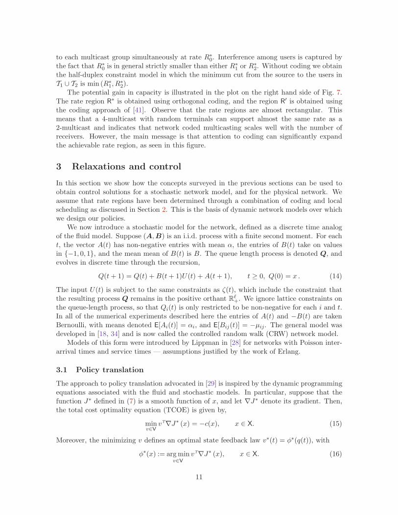
To consider the interaction among users, let T1 denote one group or receivers, and T2

another set of receivers. Consider, to begin with, orthogonal scheduling and the multicastconnections (s,T1, R

∗

1), (s,T2, R∗

2), and (s,T1 ∪ T2, R∗

0), where for each connection the rate istaken to be the maximal rate that can be supported by the network if only this particularconnection is present. We have plotted the rate points (R∗

1, 0) = (0.23, 0), (0, R∗

2) = (0, 0.24),and (R∗

0, R∗

0) = (0.21, 0.21) in Fig. 7. The extreme point (R∗

0, R∗

0) corresponds to transmission

10

to each multicast group simultaneously at rate R∗

0. Interference among users is captured bythe fact that R∗

0 is in general strictly smaller than either R∗

1 or R∗

2. Without coding we obtainthe half-duplex constraint model in which the minimum cut from the source to the users inT1 ∪ T2 is min (R∗

1, R∗

2).The potential gain in capacity is illustrated in the plot on the right hand side of Fig. 7.

The rate region R∗ is obtained using orthogonal coding, and the region R

′ is obtained usingthe coding approach of [41]. Observe that the rate regions are almost rectangular. Thismeans that a 4-multicast with random terminals can support almost the same rate as a2-multicast and indicates that network coded multicasting scales well with the number ofreceivers. However, the main message is that attention to coding can significantly expandthe achievable rate region, as seen in this figure.

3 Relaxations and control

In this section we show how the concepts surveyed in the previous sections can be used toobtain control solutions for a stochastic network model, and for the physical network. Weassume that rate regions have been determined through a combination of coding and localscheduling as discussed in Section 2. This is the basis of dynamic network models over whichwe design our policies.

We now introduce a stochastic model for the network, defined as a discrete time analogof the fluid model. Suppose (A,B) is an i.i.d. process with a finite second moment. For eacht, the vector A(t) has non-negative entries with mean α, the entries of B(t) take on valuesin {−1, 0, 1}, and the mean mean of B(t) is B. The queue length process is denoted Q, andevolves in discrete time through the recursion,

Q(t + 1) = Q(t) + B(t + 1)U(t) + A(t + 1), t ≥ 0, Q(0) = x . (14)

The input U(t) is subject to the same constraints as ζ(t), which include the constraint thatthe resulting process Q remains in the positive orthant R

ℓ+. We ignore lattice constraints on

the queue-length process, so that Qi(t) is only restricted to be non-negative for each i and t.In all of the numerical experiments described here the entries of A(t) and −B(t) are takenBernoulli, with means denoted E[Ai(t)] = αi, and E[Bij(t)] = −µij. The general model wasdeveloped in [18, 34] and is now called the controlled random walk (CRW) network model.

Models of this form were introduced by Lippman in [28] for networks with Poisson inter-arrival times and service times — assumptions justified by the work of Erlang.

3.1 Policy translation

The approach to policy translation advocated in [29] is inspired by the dynamic programmingequations associated with the fluid and stochastic models. In particular, suppose that thefunction J∗ defined in (7) is a smooth function of x, and let ∇J∗ denote its gradient. Then,the total cost optimality equation (TCOE) is given by,

minv∈V

vT∇J∗ (x) = −c(x), x ∈ X. (15)

Moreover, the minimizing v defines an optimal state feedback law v∗(t) = φ∗(q(t)), with

φ∗(x) := arg minv∈V

vT∇J∗ (x), x ∈ X. (16)

11

Similar equations define optimal policies for the CRW model with respect to a discount oraverage-cost optimality criteria [34, 2]. Generally, if h : R

ℓ → R+ is a C1 function then wedefine the h-myopic policy via

φ(x) = arg minv∈V

vT∇h (x), x ∈ X,

so that φ = φ∗ if h = J∗. It is assumed throughout that h is convex, monotone, and vanishesonly at the origin. Under these assumptions it is known that the h-myopic policy is stabilizingfor the fluid model when ρ• < 1 [34].

Router

α

Figure 8: Packets willbe routed from bufferthree to buffer fourunder the MaxWeightpolicy, for some val-ues of Q(t).

It would be tempting to attempt to apply an h-myopic policy to theCRW model, with h an approximation to the solution to an optimalityequation for the CRW model, such as the fluid value function. However,this fails because the policy might not be feasible for the stochastic model.The problem is that in the fluid model it is possible to have service atan empty buffer, which is impossible in a discrete-time CRW model.However, the situation is not so dire — there are many examples offunctions h for which the h-myopic policy is feasible for the CRW model.

The MaxWeight policy provides one example. If h(x) = 12‖x‖

2, thenthe resulting h-myopic policy coincides with the MaxWeight policy forthe models considered in [40, 39, 37, 16]. The MaxWeight policy has beenpopular for scheduling and routing in view of its stability properties. Re-cent work has developed decentralized implementations of these policiesusing consensus-type algorithms (see [35]) and distributed spanning treeconstructions (see [15]).

Many generalizations have been proposed, including a more generalquadratic h(x) = 1

2xT Dx with D > 0 diagonal, or the generalization

h(x) =∑

dix1+δi (17)

with δ > 0 and di > 0 for each i. These generalizations and more recentrefinements introduced in [16, 6, 42] are used to improve the performanceof the policy with respect to delay. Results from experiments show thatsignificant gains are possible by including additional global information,such as information regarding shortest paths to desired destinations.

Indeed, it has been observed that delay can be large when using the MaxWeight policy.An explanation was provided in [38] using the network model shown in Fig. 8 as an example.A centralized routing algorithm intended to minimize delay would never route any packetsto buffer 4. Though stabilizing, the MaxWeight algorithm will route packets to buffer 4 forcertain values of the queue length vector. This will definitely increase the average delay.

To obtain a broader class of functions for which the h-myopic policy is feasible for theCRW model, and also stabilizing, consider again the function defined in (17). Under generalconditions, the h-MaxWeight policy is feasible for the CRW model when δ > 0, while feasi-bility typically fails when δ = 0 (the case in which h is linear). The explanation given in [29]is that the function h satisfies the following boundary conditions when δ is strictly positive:

∂

∂xih (x) = 0 whenever xi = 0. (18)

12

Under these assumptions on h, including the boundary condition (18), the resulting h-myopicpolicy is called the h-MaxWeight policy in [34, 29]. This boundary condition is interpretedas zero ‘marginal disutility’ at an empty buffer, which ensures that there is a disincentive towork on an empty queue. This property is the key for stability because starvation of resourcesis avoided.

The condition (18) is easy to arrange. Suppose that h0 : Rℓ → R+ is any function satisfying

the assumptions imposed above: h0 is convex, monotone, and vanishes only at the origin.We can then perturb this function to obtain a function satisfying (18), while maintainingthe other desirable properties. One class of perturbations is of the form h(x) = h0(x) wherex = (x1, . . . , xℓ)

T ∈ Rℓ+, and each xi(x) is convex, monotone, and vanishes only at the origin.

Two examples are the exponential and logarithmic perturbations: For a given parameterθ > 0 these are defined by, respectively,

xi := xi + θ(e−xi/θ − 1) (19)

xi := xi log(1 + xi/θ) (20)

Feasibility of the h-MaxWeight policy requires some assumptions on the velocity set V.One set of sufficient conditions is given in Proposition 3.1.

Proposition 3.1. Suppose that the following hold for the general fluid model:

(i) ρ• < 1.

(ii) For any v ∈ V and any i ∈ {1, . . . , ℓ}, if vi < 0 then there is a vector v+ ∈ V

satisfyingv+i = 0 and v+

j ≤ vj for j 6= i.

Then without loss of generality, the h-myopic policy can be constructed so that for any x ∈ Rℓ+,

and any i, we have φi(x) ≥ 0 when xi = 0.

Proof. By definition we have

φ(x) ∈ arg minv∈V

ℓ∑

i=1

vi∂

∂xih (x), x ∈ X.

If v0 achieves the minimum, then there exists v+ satisfying v+i = 0 whenever xi = 0 and

vi < 0, and v+j ≤ vj otherwise. Monotonicity of h implies that v0T

∇h (x) ≥ v+T∇h (x). ⊓⊔

To see how this applies to policy translation, we show how to translate an optimal policyfor the fluid model relaxation to the CRW model. The translation is performed in two steps.In the first step we modify the value function for the relaxation. For a one-dimensionalrelaxation, and with linear cost, the value function J∗ is a quadratic function of workloadw = ξTx. To attempt to faithfully track the relaxation we introduce a penalty term thatintroduces a large cost when c(x) ≫ c(w):

h0(x) := J∗(w) +b

2

(c(x) − c(w)

)2, w = ξTx, x ∈ R

ℓ+, (21)

where b > 0 is a constant. In the second step we perturb h0 to obtain h satisfying (18).

13

It is shown in [29] that the resulting h-MaxWeight policy is approximately optimal undergeneral conditions. While the arguments are general, this result is proven for a versionof the scheduling model described below eq. (4). Note however that to obtain such exactperformance guarantees it is necessary to demand far greater information than using thestandard MaxWeight policy. In practice tradeoffs must be made between information andperformance. Moreover, network structure may change with time, in which case the policymust adapt to these changes.

3.2 h-MaxWeight for dynamic routing

In this final section we describe how these techniques apply to networks found in telecommu-nication applications.

Fig. 9 shows a network with 100 nodes, two arrival streams, and one node from whichthe packets from these two sources exit the network. The network was constructed by firstselecting at random the positions of nodes. A link between two nodes was created wheneverthe distance was less than a threshold. These links were chosen to be uni-directional, andeach direction was also randomly selected. The capacity on a link between nodes i and j isdenoted µij . Its value was set to one of four possible values: 0.5,0.25,0.2 or 0.15. Generally,smaller rates were assigned for links in the central region of the network.

The two dashed lines shown in Fig. 9 represent a single cut between the two inflows,and the single outflow. The total number of packets in the shaded region coincides with theworkload (in units of packets) corresponding to this cut.

Figure 9: A network with 100 nodes. There are four classes of links, differentiated by their capacity, andindicated in the figure by the four different styles shown. The rates of links for the solid, dashed, dotted anddash-dot lines are 0.5,0.25,0.2 and 0.15 respectively. The two arrivals and one exit are indicated by the arrows.

In all of the numerical experiments described here, the arrival process A = {A(t) : t ≥ 1}was taken to be an i.i.d. sequence with distribution,

P (Ai(t) = n) = αi/n, P (Ai(t) = 0) = 1 − αi/n, 1 ≤ i ≤ 2 (22)

where n is a constant used to capture variability. The mean and variance of Ai(t) are givenby, respectively,

mAi(t) = αi, σ2Ai(t)

= nαi − α2i . (23)

14

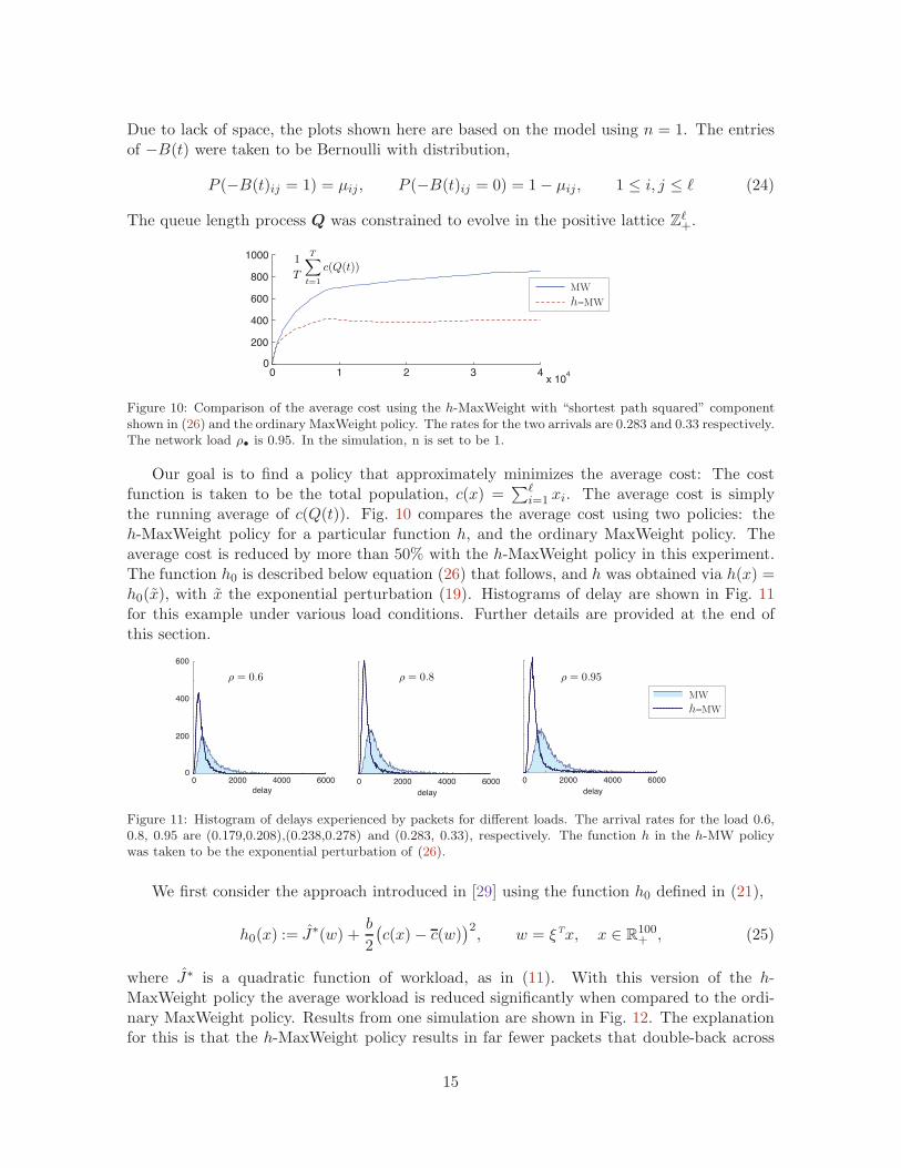
Due to lack of space, the plots shown here are based on the model using n = 1. The entriesof −B(t) were taken to be Bernoulli with distribution,

P (−B(t)ij = 1) = µij, P (−B(t)ij = 0) = 1 − µij, 1 ≤ i, j ≤ ℓ (24)

The queue length process Q was constrained to evolve in the positive lattice Zℓ+.

1

T

T

t=1

c(Q(t))

MW

h−MW

0

200

400

600

800

1000

x 1040 1 2 3 4

Figure 10: Comparison of the average cost using the h-MaxWeight with “shortest path squared” componentshown in (26) and the ordinary MaxWeight policy. The rates for the two arrivals are 0.283 and 0.33 respectively.The network load ρ• is 0.95. In the simulation, n is set to be 1.

Our goal is to find a policy that approximately minimizes the average cost: The costfunction is taken to be the total population, c(x) =

∑ℓi=1 xi. The average cost is simply

the running average of c(Q(t)). Fig. 10 compares the average cost using two policies: theh-MaxWeight policy for a particular function h, and the ordinary MaxWeight policy. Theaverage cost is reduced by more than 50% with the h-MaxWeight policy in this experiment.The function h0 is described below equation (26) that follows, and h was obtained via h(x) =h0(x), with x the exponential perturbation (19). Histograms of delay are shown in Fig. 11for this example under various load conditions. Further details are provided at the end ofthis section.

ρ = 0.6 ρ = 0.8 ρ = 0.95

0 2000 4000 6000

delay

0 2000 4000 6000

delay

0 2000 4000 60000

200

400

600

delay

MW

h−MW

Figure 11: Histogram of delays experienced by packets for different loads. The arrival rates for the load 0.6,0.8, 0.95 are (0.179,0.208),(0.238,0.278) and (0.283, 0.33), respectively. The function h in the h-MW policywas taken to be the exponential perturbation of (26).

We first consider the approach introduced in [29] using the function h0 defined in (21),

h0(x) := J∗(w) +b

2

(c(x) − c(w)

)2, w = ξTx, x ∈ R

100+ , (25)

where J∗ is a quadratic function of workload, as in (11). With this version of the h-MaxWeight policy the average workload is reduced significantly when compared to the ordi-nary MaxWeight policy. Results from one simulation are shown in Fig. 12. The explanationfor this is that the h-MaxWeight policy results in far fewer packets that double-back across

15

0 1 2 3 4x 10

4 0 1 2 3 4x 10

4

0 1 2 3 4x 10

4 0 1 2 3 4x 10

4

0

200

400

600

800

1000

0

200

400

600

800

1000

0

200

400

600

800

1000

0

200

400

600

1

T

T

t=1

c(Q(t))1

T

T

t=1

W (t)

1

T

T

t=1

c(Q(t)) − c(W (t))

T

t=1

L(t)

MW

h−MW

Figure 12: Simulation results for the h-Maxweight using the exponential perturbation of the function h0 givenin (25).

the network cut. Denote by L(t) the number of packets that cross the cut in the upstreamdirection at time t ≥ 0. The cumulative sum of this quantity was obtained for the two poli-cies, and the results are shown in Fig. 12. It is seen that the number of “loopy packets” isreduced by approximately one half when compared to the MaxWeight policy.

However, there is one aspect of this policy that is not satisfactory. Recall that an optimalsolution for the workload relaxation requires c(Q(t)) − c(W (t)) ≡ 0 for t > 0. The errorc(Q(t)) − c(W (t)) is proportional to the number of packets downstream of the network cut.Hence, in an optimal solution for the relaxation, all nodes downstream of the network cut befree of packets. The running average of c(Q(t)) − c(W (t)) was obtained for the two policies,and the results are also displayed in Fig. 12. We see that the result is similar for either policy,and the average value is approximately half of the total average cost.

To better approximate the idealization c(Q(t)) − c(W (t)) ≡ 0, we now introduce anadditional penalty term in h0 to more aggressively move traffic towards the exit node. Theidea is to introduce information regarding the shortest path to the exit, following a similarmodification of the MaxWeight policy introduced in [42]. For each i, denote by s(i) thelength (in hops) of the shortest path from node i to the exit node. For a given p > 0, thecorresponding vector of powers of {s(i)} is denoted by dsp = [s(1)p, s(2)p, . . . , s(ℓ)p]T . Thedefinition of h0 in (21) is then modified to include the linear function of x obtained as thedot product with dsp:

h0(x) := J∗(w) +b

2

(c(x) − c(w)

)2+ bspd

spT x, w = ξTx, x ∈ R100+ , (26)

where bsp is a constant.Fig. 13 shows results obtained under the same conditions as described following Fig. 10,

but using this function in the definition of the h-MaxWeight policy, with p = 2 (so thatdsp

i = s(i)2). The average value of c(Q(t)) − c(W (t)) is reduced by nearly one half, ascompared to the previous version of the h-MaxWeight policy.

In each simulation the delay for each packet entering the network was also recorded. Thisis the total time from arrival to the network, to the time of exit from the network. Histogramsof delay are shown in Fig. 11. This includes the network under the same statistical setting

16

0 1 2 3 4x 10

4 0 1 2 3 4x 10

4

0 1 2 3 4x 10

4 0 1 2 3 4x 10

4

0

200

400

600

800

1000

0

200

400

600

800

1000

0

200

400

600

800

1000

0

200

400

600

1

T

T

t=1

c(Q(t))1

T

T

t=1

W (t)

1

T

T

t=1

c(Q(t)) − c(W (t))T

t=1

L(t)

MW

h−MW

Figure 13: Simulation results for the h-Maxweight with shortest path component. The solid line shows resultfor the MaxWeight policy, while the dashed line shows the result for the h-MaxWeight with “shortest pathsquared” component shown in (26).

as in the prior experiments, with network load ρ• = 0.95. Two other experiments wereconducted with reduced arrival rates, resulting in loads ρ• = 0.6 and 0.8. The averagedelay, and the variability of delay are reduced dramatically using this policy, as compared toordinary MaxWeight.

4 Conclusions

We have seen that a careful look at deterministic aspects of a communication network canprovide insight regarding network control, as well as practical algorithms. As illustrated byexamples, it is possible to develop models and solutions for broad classes of networks, andtake into account many network issues, including those related to multiple access interferenceand coding.

There are many promising directions for future research; we highlight just two — theinterplay between network control and information theory, and the decentralized implemen-tation of network algorithms.

Information theory characterizes the fundamental gains and limits of coding, while net-work control is concerned primarily with policies and performance bounds. Information the-ory is an indispensable tool to guide the design of network algorithms; however, techniquesfrom information theory have only recently begun to have impact on communication networkdesign. This tension between the two disciplines (the unconsummated union [12]), is yet tobe resolved in a satisfactory way. Working from both directions to create a more cohesivebridge is a very promising avenue of further research. The applications described here tomultiple access communication and network coded multicasting are just two examples.

The second direction concerns the decentralized implementation of network control al-gorithms. Centralized coordination is limited in most wireless networks owing to physicallimitations and choice of architecture. There have been two recent approaches for designingdecentralized network control algorithms. The first approach uses insights from game theoryto design dynamic update mechanisms among users competing for network resources (see forexample [7]). While being fully decentralized and flexible in modeling heterogeneous user

17

metrics, this approach may lead to inefficiencies in the overall network performance due tostrategic interactions among users. In environments where there are no strategic interactions,a more direct approach can be used that relies on optimization decomposition methods andconsensus algorithms. Some of the techniques described in the paper, in particular networkcoding for multicasting, can be naturally decentralized using this approach. The constructionof decentralized implementations of the h-MaxWeight policy is also possible using consensusalgorithms, but the need for high reliability and efficiency will drive further research in thisdirection.

References

[1] R. Ahlswede, N. Cai, S.-Y. R. Li, and R. W. Yeung. Network information flow. IEEETransactions on Information Theory, 46:1024–1016, 2000.

[2] D. P. Bertsekas. Dynamic Programming and Optimal Control. Athena Scientific, thirdedition, 2007.

[3] D. Bertsimas and J. Nino-Mora. Restless bandits, linear programming relaxations, anda primal-dual index heuristic. Operations Res., 48(1):80–90, 2000.

[4] M. Bramson and R. J. Williams. Two workload properties for Brownian networks.Queueing Syst. Theory Appl., 45(3):191–221, 2003.

[5] E. Brockmeyer, H.L. Halstrøm, and A. Jensen. The life and works of A.K. Erlang. TheCopenhagen Telephone Company, Copenhagen, 1948.

[6] L. Bui, R. Srikant, and A. Stolyar. Novel architectures and algorithms for delay re-duction in back-pressure scheduling and routing. ArXiv Computer Science e-prints.arXiv:0901.1312. A short version of this paper is accepted to the INFOCOM 2009 Mini-Conference, Jan 2009.

[7] U.O. Candogan, I. Menache, A. Ozdaglar, and P.A. Parrilo. Competitive scheduling inwireless collision channels with correlated channel state. In Proceeedings of the Interna-tional Conference on Game Theory for Networks (GameNets), 13-15 May 2009.

[8] W. Chen, D. Huang, A. Kulkarni, J. Unnikrishnan, Q. Zhu, P. Mehta, S. Meyn, andA. Wierman. Approximate dynamic programming using fluid and diffusion approxima-tions with applications to power management. Submitted to the 48th IEEE Conferenceon Decision and Control, December 16-18 2009.

[9] E. G. Coffman Jr. and I. Mitrani. A characterization of waiting times realizable by singleserver queues. Operations Res., 28:810–821, 1980.

[10] T. M. Cover. Comments on broadcast channels. IEEE Trans. Inform. Theory,44(6):2524–2530, 1998. Information theory: 1948–1998.

[11] T. M. Cover and J. A. Thomas. Elements of information theory. John Wiley & SonsInc., New York, 1991. A Wiley-Interscience Publication.

18

[12] A. Ephremides and B. E. Hajek. Information theory and communication networks: Anunconsummated union. IEEE Trans. Inform. Theory, 44(6):2416–2434, 1998.

[13] A. K. Erlang. Solution of some problems in the theory of probabilities of significancein automatic telephone exchanges. In E. Brockmeyer, H.L. Halstrøm, and A. Jensen,editors, The life and works of A.K. Erlang, pages 189–. The Copenhagen TelephoneCompany, Copenhagen, 1948. Originally published in Danish in Elektrotkeknikeren, vol13, 1917.

[14] A. K. Erlang. The theory of probabilities and telephone conversations. In E. Brockmeyer,H.L. Halstrøm, and A. Jensen, editors, The life and works of A.K. Erlang, pages 131–. The Copenhagen Telephone Company, Copenhagen, 1948. Originally published inDanish in Nyt Tidsskrift for Matematik B, 1909.

[15] A. Eryilmaz, A. Ozdaglar, and E. Modiano. Polynomial complexity algorithms for fullutilization of multihop wireless networks. In Proceeedings of IEEE INFOCOM, 2007.

[16] L. Georgiadis, M. Neely, and L. Tassiulas. Resource Allocation and Cross Layer Con-trol in Wireless Networks (Foundations and Trends in Networking, V. 1, No. 1). NowPublishers Inc., Hanover, MA, USA, 2006.

[17] G. R. Gupta and N. B. Shroff. Delay analysis for multi-hop wireless networks. InProceedings of IEEE Infocom, Rio de Janeiro, Brazil, 2009. Presentation given at ITA-Workshop 2009, UCSD.

[18] S. G. Henderson, S. P. Meyn, and V. B. Tadic. Performance evaluation and policyselection in multiclass networks. Discrete Event Dynamic Systems: Theory and Applica-tions, 13(1-2):149–189, 2003. Special issue on learning, optimization and decision making(invited).

[19] T. Ho, M. Medard, M. Effros, and D. Karger. On randomized network coding. In Proc.41st Allerton Annual Conference on Communication, Control and Computing, October2003.

[20] T. Ho, M. Medard, R. Koetter, D.R. Karger, M. Effros, Jun Shi, and B. Leong. A randomlinear network coding approach to multicast. Information Theory, IEEE Transactionson, 52(10):4413–4430, Oct. 2006.

[21] S. Jaggi, P. Sanders, P.A. Chou, M. Effros, S. Egner, K. Jain, and L.M.G.M. Tolhuizen.Polynomial time algorithms for multicast network code construction. Information The-ory, IEEE Transactions on, 51(6):1973–1982, June 2005.

[22] F. W. Johannsen. Waiting times and number of calls. P.O. Electrical Engineers Journal,1907.

[23] F.P. Kelly and C.N. Laws. Dynamic routing in open queueing networks: Brownianmodels, cut constraints and resource pooling. Queueing Syst. Theory Appl., 13:47–86,1993.

[24] L. Kleinrock. Queueing Systems Vol. 1: Theory. Wiley, 1975.

19

[25] P. R. Kumar and S. P. Meyn. Duality and linear programs for stability and performanceanalysis queueing networks and scheduling policies. IEEE Trans. Automat. Control,41(1):4–17, 1996.

[26] S. Kumar and P. R. Kumar. Performance bounds for queueing networks and schedulingpolicies. IEEE Trans. Automat. Control, AC-39:1600–1611, August 1994.

[27] N. Laws. Dynamic routing in queueing networks. PhD thesis, Cambridge University,Cambridge, UK, 1990.

[28] S. Lippman. Applying a new device in the optimization of exponential queueing systems.Operations Res., 23:687–710, 1975.

[29] S. Meyn. Stability and asymptotic optimality of generalized MaxWeight policies. SIAMJ. Control Optim., 47(6):3259–3294, 2009.

[30] S. P. Meyn. The policy iteration algorithm for average reward Markov decision processeswith general state space. IEEE Trans. Automat. Control, 42(12):1663–1680, 1997.

[31] S. P. Meyn. Stability and optimization of queueing networks and their fluid models.In Mathematics of stochastic manufacturing systems (Williamsburg, VA, 1996), pages175–199. Amer. Math. Soc., Providence, RI, 1997.

[32] S. P. Meyn. Sequencing and routing in multiclass queueing networks. Part II: Workloadrelaxations. SIAM J. Control Optim., 42(1):178–217, 2003.

[33] S. P. Meyn. Dynamic safety-stocks for asymptotic optimality in stochastic networks.Queueing Syst. Theory Appl., 50:255–297, 2005.

[34] S. P. Meyn. Control Techniques for Complex Networks. Cambridge University Press,Cambridge, 2007.

[35] E. Modiano, D. Shah, and G. Zussman. Maximizing throughput in wireless networksvia gossiping. In Proceeedings of ACM Sigmetrics/IFIP Performance, 2006.

[36] D. Shah and D. Wischik. Lower bound and optimality in switched networks. In Proceed-ings of the 46th Annual Allerton Conference on Communication, Control, and Comput-ing, pages 1262–1269, Sept. 2008.

[37] R. Srikant. The mathematics of Internet congestion control. Systems & Control: Foun-dations & Applications. Birkhauser Boston Inc., Boston, MA, 2004.

[38] V. Subramanian and D. Leith. Draining time based scheduling algorithm. In Proceedingsof the 46th IEEE Conf. on Decision and Control, pages 1162–1167, 2007.

[39] L. Tassiulas and A. Ephremides. Jointly optimal routing and scheduling in packet radionetworks. IEEE Trans. Inform. Theory, 38(1):165–168, 1992.

[40] L. Tassiulas and A. Ephremides. Stability properties of constrained queueing systemsand scheduling policies for maximum throughput in multihop radio networks. IEEETrans. Automat. Control, 37(12):1936–1948, 1992.

20

[41] D. Traskov, M. Heindlmaier, M. Medard, R. Koetter, and D.S. Lun. Scheduling fornetwork coded multicast: A conflict graph formulation. In Proceedings of the IEEEGLOBECOM Workshop, pages 1–5, 2008.

[42] L. Ying, S. Shakkottai, and A. Reddy. On combining shortest-path and back-pressurerouting over multihop wireless networks. In Proceedings of IEEE Infocom, Rio de Janeiro,Brazil, April 2009.

21