code development for control design applications phase … · nrel/cp-500-25792 code development...

NREL/CP-500-25792

Code Development forControl Design Applications

Phase I: Structural Modeling

Gunjit S. Bir, Michael RobinsonNational Wind Technology CenterNational Renewable Energy Laboratory

Presented atAIAA/ASME Wind Energy SymposiumReno, NevadaJanuary 11−14, 1999

National Renewable Energy Laboratory1617 Cole BoulevardGolden, Colorado 80401-3393A national laboratory of the U.S. Department of EnergyManaged by Midwest Research Institutefor the U.S. Department of Energyunder contract No. DE-AC36-83CH10093

Work performed under task number WE901430

November 1998

NOTICE

This report was prepared as an account of work sponsored by an agency of the United States government.Neither the United States government nor any agency thereof, nor any of their employees, makes anywarranty, express or implied, or assumes any legal liability or responsibility for the accuracy,completeness, or usefulness of any information, apparatus, product, or process disclosed, or representsthat its use would not infringe privately owned rights. Reference herein to any specific commercial product,process, or service by trade name, trademark, manufacturer, or otherwise does not necessarily constituteor imply its endorsement, recommendation, or favoring by the United States government or any agencythereof. The views and opinions of authors expressed herein do not necessarily state or reflect those of theUnited States government or any agency thereof.

Available to DOE and DOE contractors from:Office of Scientific and Technical Information (OSTI)P.O. Box 62Oak Ridge, TN 37831

Prices available by calling (423) 576-8401

Available to the public from:National Technical Information Service (NTIS)U.S. Department of Commerce5285 Port Royal RoadSpringfield, VA 22161(703) 487-4650

Printed on paper containing at least 50% wastepaper, including 20% postconsumer waste

AIAA-99-0032

1American Institute of Aeronautics and Astronautics

1

Code Development for Control Design Applications(Phase I: Structural Modeling)

Gunjit S. BirMichael Robinson

National Wind Technology CenterNational Renewable Energy Laboratory

1617 Cole Boulevard, Golden, CO 80401

ABSTRACT

The design of integrated controls for a complexsystem like a wind turbine relies on a system modelin an explicit format, e.g., state-space format.Current wind turbine codes focus on turbinesimulation and not on system characterization,which is desired for controls design as well asapplications like operating turbine modal analysis,optimal design, and aeroelastic stability analysis.We initiated development of a specialized code toprovide explicit system models. The code drawsheavily from modern multibody modeling conceptsas well as advanced features of an existing helicoptercode. The code will be implemented in two phases:structural modeling followed by aerodynamicmodeling. This paper* reviews structural modelingthat comprises three major steps: formulation ofcomponent equations, assembly into systemequations, and linearization. Linearization providessystem equations in descriptive formats, clearlydelineating linear and nonlinear parts, which canthen be readily used by optimal control schemes.

INTRODUCTION

A wind turbine is a complex machine that operatesunder severe dynamic and aerodynamic conditions.A multi-input multi-output control system offers thepotential to coordinate machine component functionsand improve performance, fatigue life, and stability.Central to integrated control efforts is the availabilityof wind turbine explicit models. Examples ofexplicit models are state-space models, finite elementmodels, and modal models. An explicit model alsoseparates linear and nonlinear parts of systemgoverning equations in forms that can be readilyintegrated into systematic control design schemes.Currently available wind turbine codes, e.g.ADAMS1, FAST2, and YawDyn3, have beensuccessfully used to model a broad range of wind * This paper is declared a work of the U.S. Government and is notsubject to copyright protection in the United States.

turbines. However, these codes rely on implicitformulation that is adequate for simulation but notfor designing controllers, computing operatingmodes, and other important applications. ADAMShas comprehensive modeling capabilities and cangenerate a first-order explicit state-space model.However, a state-space model can be extracted onlyfor a non-operating (parked) wind turbine. Theaccuracy of the model deteriorates rapidly as therotor speed increases. Another limitation is that theextracted model offers only numerical informationand not symbolic information, in terms of systemparameters and degrees of freedom, that helps covera wider range of design and operating conditions.System identification techniques may be used toextract low-order models4 from simulation codes.These techniques, however, provide only single-operation-specific numerical information and requirean inordinate amount of time and systemidentification expertise. Also, the fidelity of suchmodels is limited only to the first few system modes.For a complex system like a wind turbine, suchidentified models may not capture system cross-couplings, e.g., yaw-flap-pitch, with the accuracyrequired for multi-input multi-output controlsdesign. Models extracted via system identificationtherefore may at best be used for simple applications,e.g., power regulation or flap loads alleviation alone.

We initiated development of a specialized code tocomplement existing turbine codes and provideexplicit system descriptive models. The code drawsfrom newly developed flexible multibody modelingtechniques5,6 and selective features of an advancedhelicopter code called UMARC7, that is wellvalidated and extensively used in the helicopter field.Adaptation of sophisticated features from thehelicopter code such as a finite element techniquespecialized to rotating blade, multiblade coordinatetransformation, and Floquet analysis of periodicsystems, would save us several years of developmentand validation efforts. A detailed rationale behindthis approach for code development and associated

AIAA-99-0032


2

modeling issues were presented8 at the 1998Windpower conference held in Bakersfield,California. The code will be developed in twophases: phase I will cover structural modeling andphase II will cover full aeroelastic modeling.

This paper reviews our effort under way on structuralmodeling. We first describe wind turbine structuralidealization, which forms the basis for all subsequentderivations. We then derive turbine componentequations of motion. Next, the component equationsare assembled to satisfy inter-component force anddisplacement constraints. This is followed bylinearization of the system equations andtransformation into explicit formats.

WIND TURBINE IDEALIZATION

We idealize the turbine structure by replacing it withan assemblage of flexible and rigid bodies joined byactuator elements and constraints, some of whichmay be time-variant. Each of these bodies mayundergo large rotational and translational motions.The blades are idealized as rotating flexible beams,which may be single-path (for conventional blades)or multiple-path (for blades with multiple spars andlinkages that transmit loads to the hub). Each beamundergoes flap bending, lag bending, elastic twistand axial deflection, and may have arbitraryspanwise distributions of mass, section inertia,flexural stiffness, torsion stiffness, built-in twist, andoffsets amongst the elastic axis, the centers-of-massaxis and the tension-centers axis. The hub, thegenerator, the nacelle, the gearbox inertia, and thebed frame are treated as rigid bodies. The tower andthe drive-train shaft are treated as flexible beams.The turbine model has provisions for nonlinearspring dampers to restrain any joint motion, e.g.yaw, teeter and nacelle tilt. There are alsoprovisions for arbitrary number of blades, precone,pitch control, and delta-3 effects. This results in acomprehensive turbine model that captures all thestructural mechanisms and couplings required forhigh-fidelity loads and response analysis, stabilityevaluation, modal analysis, and controlsapplications. For detailed stress analysis at a criticallocation, which may for example be required forfatigue life calculations, loads and response outputfrom the comprehensive code may be input to anycommercial finite element code that models in detailonly a small region enclosing that location.

SYSTEM COORDINATES

Much of the current research in multibody dynamicsaddresses the selection of system generalizedcoordinates that describe time-dependent systemconfiguration. The selection profoundly effects theefficacy of each of the three major steps involved insystem modeling, i.e., component modeling,assembly, and linearization. A trade-off must bemade between the generality and the efficiency of thedynamic formulation. For example, the choice ofabsolute coordinates, wherein all the degrees offreedom are referred to a single inertial frame,makes the assembly process trivial; however, for asystem with rotating parts, it leads to erroneouslinearization. Incorrect linearization results becausesome important centrifugal terms, that depend onrotational speed and are linear when referred to arotating natural frame, become nonlinear whenreferred to the inertial frame, and linearization dropsthese terms. That is why ADAMS offers excellentsimulation capabilities that rely on assembledequations, but fails to provide correct system modesthat rely on linearized equations. The choice ofcoordinates has an even more pronounced effect onthe number of system equations, the simplicity ofeach equation, computability of constraint forces,numerical conditioning of equations, and theefficiency of the solution procedures. We made andare still making effort to study these issues as best aswe can. Once we have conclusive results, a reportwould follow. Basically, for multi-rigid-bodydynamic modeling, we have three choices for systemcoordinates: absolute configuration coordinates, jointvariables, and generalized speeds.

The choice of absolute coordinates leads to similar-looking equations for each body and makes assemblystraightforward. This choice, however, leads to anonminimal number of system equations. For asystem with n degrees of freedom and m constraints,the number of nonminimal system equations wouldbe n+2m which comprise n+m differential equationsassociated with the n+m absolute generalizedcoordinates, and m algebraic equations associatedwith the m constraints. These equations are solvedfor the n+m absolute coordinates and m Lagrangemultipliers associated with the constraint forces.The resulting mixed set of differential-algebraicequations, however, is extremely difficult to solveaccurately and a special technique, like the oneproposed by Wehage9, must be employed. The extra2m equations also make this choice computationallyexpensive. Coordinate partitioning may be used toeliminate the dependent coordinates; however, this

AIAA-99-0032


3

can be a tricky process. The second choice, jointvariables, wherein the system equations of motionare written in terms of joint degrees of freedom,leads to a minimal set of differential equations andhence substantial computational time savings.However, it requires relatively complex constraint-specific recursive formulation. This approach is stilldesirable since it leads to linear equations that yielda correct eigensolution for a system with rotatingparts. The third choice for system coordinates is touse generalized speeds10, defined as a linearcombination of time derivatives of generalizedcoordinates. This also leads to a minimal set ofequations since the constraints are implicitly takencare of during formulation. This choice also has thepotential to yield efficient simple equations providedthe generalized speeds are defined rightly to suitgiven constraints. The choice also is system-configuration-specific and does not permit theautomatic assembly required for a general system.Also, an efficient interface of the rigid-bodysubassembly with the elastic-body subassembly isstill an open research area.

Compared with rigid body dynamics, the selection ofcoordinates for flexible body dynamics presents anumber of conceptual problems. Exact modeling ofan elastic body requires infinite degrees of freedom.Therefore, the first problem is the definition of anacceptable model for the elastic body using a finiteset of coordinates. In the Rayleigh-Ritz method, thisproblem is solved by assuming that the shape of thedeformed body with respect to a reference frame canbe approximated through a finite set of a specificclass of functions. The finite element method is onetype of Raleigh method in which the elastic body isdiscretized into a number of regions connected bynodes. The deformation of the elastic body withrespect to a reference frame is expressed in terms ofshape functions and nodal degrees of freedomassociated with each region called an element. Theefficacy of the finite element formulation depends toa large extent on the nature of the element nodalcoordinates. This is still a field of extensive researchand a number of methods have been proposed whichcan be roughly classified into three basicformulations: the floating reference frame offormulation, the incremental formulation, and thelarge rotation vector formulation. Shabana11

provides an excellent discussion of these methods

We select joint variables for rigid bodies since itleads to a minimal set of system equations and alsocorrect linearization. For the elastic bodies, weselect a floating frame of reference formulation

wherein a coordinate system is assigned to eachdeformable body. The large rotation and translationof the deformable body are defined in terms of theabsolute motion of the body-attached referenceframe; this absolute motion in turn is expressedrecursively in terms of joint coordinates. Thedeformation of the body with respect to its referenceframe is expressed in terms of the elements’ nodalcoordinates. It can be demonstrated that this choiceleads to exact modeling of the rigid body inertiawhen there is no deformation. However, thedeformation of the body is assumed to be moderate.This assumption is valid for wind turbine elasticcomponents and allows substantial simplification ofthe governing equations.

COMPONENT EQUATIONS

Basic to full system modeling is the derivation ofequations governing its components. From thesection on wind turbine idealization it follows thatany component of the wind turbine may be modeledeither as a flexible beam or as a rigid body.

For the flexible beam, Hamilton's variationalprinciple is used to derive component equations ofmotion. For a non-conservative system, thisprinciple is expressed as

( )∫ =−−=2

1

0t

t

dtWTU δδδδπ (1)

where Uδ is the virtual variation of potentialenergy, Tδ is the virtual variation of kinetic energy,and Wδ is the virtual work done by external forces,e.g., aerodynamic forces, which are not derivablefrom a potential function. The virtual variation inthe strain energy is given by

( )[ ]∫ ∫∫ •+++=L

oA

QIxxxxxxxx dxddRgU ζηδρδεσδεσδεσδ ζζηη

vv

( )[ ]∫ ∫∫ •+++Ε=L

oA

QIxxxxxxxx dxddRgGG ζηδρδεεδεεδεε ζζηη

vv

(2)The strain components xxε , ηε x , ζε x are functions

of the beam extensional deflection u , bendingdeflections ν and w , the elastic twist φ , and theirspatial derivatives. The explicit expressions forthese strains are derived by considering theorientation of a generic coordinate triad ( )ζηξ ,, ,attached to the principal axes of a cross section ofthe deformed blade, with respect to the ( )zyx ,,coordinate triad attached to the undeformed blade.

AIAA-99-0032


4

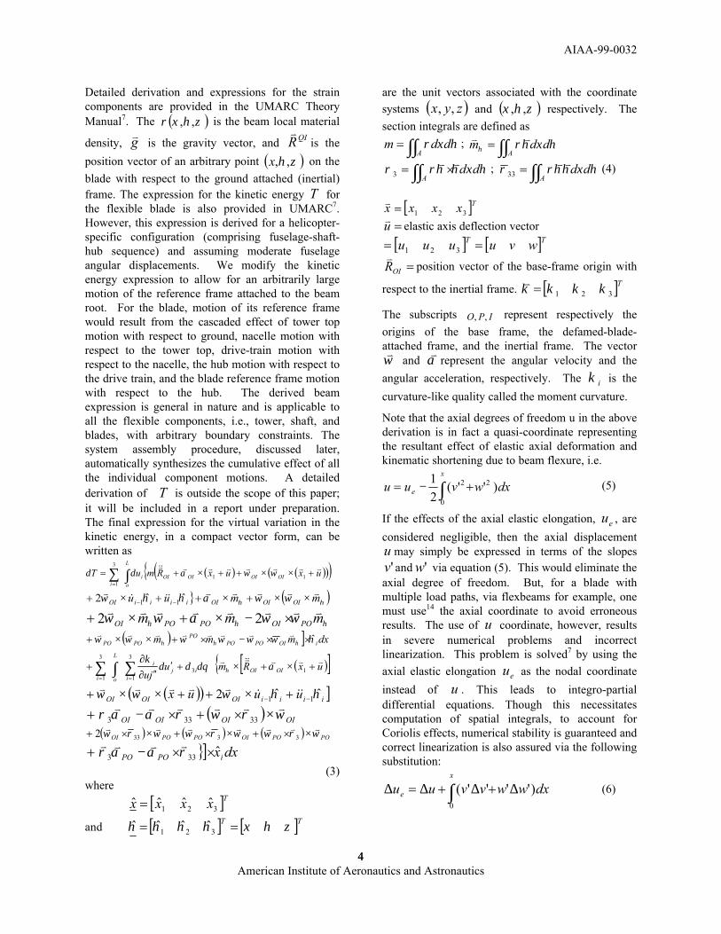
Detailed derivation and expressions for the straincomponents are provided in the UMARC TheoryManual7. The ( )ζηξρ ,, is the beam local material

density, gv is the gravity vector, and QIRv

is theposition vector of an arbitrary point ( )ζη,,x on theblade with respect to the ground attached (inertial)frame. The expression for the kinetic energy T forthe flexible blade is also provided in UMARC7.However, this expression is derived for a helicopter-specific configuration (comprising fuselage-shaft-hub sequence) and assuming moderate fuselageangular displacements. We modify the kineticenergy expression to allow for an arbitrarily largemotion of the reference frame attached to the beamroot. For the blade, motion of its reference framewould result from the cascaded effect of tower topmotion with respect to ground, nacelle motion withrespect to the tower top, drive-train motion withrespect to the nacelle, the hub motion with respect tothe drive train, and the blade reference frame motionwith respect to the hub. The derived beamexpression is general in nature and is applicable toall the flexible components, i.e., tower, shaft, andblades, with arbitrary boundary constraints. Thesystem assembly procedure, discussed later,automatically synthesizes the cumulative effect of allthe individual component motions. A detailedderivation of T is outside the scope of this paper;it will be included in a report under preparation.The final expression for the virtual variation in thekinetic energy, in a compact vector form, can bewritten as

( ) ( )( )( ){∑ ∫=

+××++×+=

3

111

i

L

oOIOIOIOIi uxuxRmuT vvvvvvv&&v ωωαδδ

} ( )ηη ωωαηηω mmuu OIOIOIiiiiOIvvvvv

&&&v ××+×++×+ −− ˆˆ2 11

ηηη ωωαωω mmm POOIPOPOOIvvvvvvvv ×−×+×+ 22

( ) ] dxmmm iOIPOPOPO

POPO ηωωωωωω ηηη ˆ××−×+××+ vvvvvvvv

( )[ ]{∑ ∫ ∑= =

+×+×

+′′′∂

∂+

3

11

3

13

i

L

oOIOI

iij

i uxRmuju

vvv&&vv αδθδδκ

η

( )( ) ]iiiiOIOIOI uuux ηηωωω ˆˆ2 11 −− +×++××+ &&&vvvvv

( ) OIOIOIOI ωρωρααρ vvvvvv ××+×−+ 33333

( ) ( ) ( ) POPOOIPOPOOI ωρωωρωωρω vvvvvvv ××+××+××+ 33332

}] dxxiPOPO ˆ333 ××−+ ρααρvvvv

(3)where

[ ]Txxxx 321 ˆˆˆˆ =and [ ] [ ]TT ζηξηηηη == 321 ˆˆˆˆ

are the unit vectors associated with the coordinatesystems ( )zyx ,, and ( )ζηξ ,, respectively. Thesection integrals are defined as

∫∫=A

ddm ηξρ ; ∫∫=A

ddm ηξηρηvv

∫∫ ×=A

dd ηξηηρρ vv3 ; ∫∫=

Add ηξηηρρ vv

33 (4)

[ ]Txxxx 321=v

=uv elastic axis deflection vector

[ ]Tuuu 321= [ ]Twvu=

=OIRv

position vector of the base-frame origin with

respect to the inertial frame. [ ]T321 κκκκ =v

The subscripts IPO ,, represent respectively theorigins of the base frame, the defamed-blade-attached frame, and the inertial frame. The vectorωv and αv represent the angular velocity and theangular acceleration, respectively. The iκ is thecurvature-like quality called the moment curvature.

Note that the axial degrees of freedom u in the abovederivation is in fact a quasi-coordinate representingthe resultant effect of elastic axial deformation andkinematic shortening due to beam flexure, i.e.

∫ +−=x

e dxwvuu0

22 )''(21 (5)

If the effects of the axial elastic elongation, eu , areconsidered negligible, then the axial displacementu may simply be expressed in terms of the slopes'v and 'w via equation (5). This would eliminate the

axial degree of freedom. But, for a blade withmultiple load paths, via flexbeams for example, onemust use14 the axial coordinate to avoid erroneousresults. The use of u coordinate, however, resultsin severe numerical problems and incorrectlinearization. This problem is solved7 by using theaxial elastic elongation eu as the nodal coordinateinstead of u . This leads to integro-partialdifferential equations. Though this necessitatescomputation of spatial integrals, to account forCoriolis effects, numerical stability is guaranteed andcorrect linearization is also assured via the followingsubstitution:

∫ ∆+∆+∆=∆x

e dxwwvvuu0

)''''( (6)

AIAA-99-0032


5

Finite Element Discretization

Hamilton's principle (1) results in partial differentialequations for the continuous-domain flexible body.A specialized finite element technique7, developed tohandle integral-partial differential equationsassociated with rotating flexible blades, is used tospatially discretize the governing equations into afinite set of N ordinary differential equations in time,where N is the number of generalized coordinatesrepresenting the finite element modal degrees offreedom. Each flexible component (tower, shaft, orblade) is divided into a number of 15-degrees offreedom beam elements (Figure 1). The finiteelement assembly process ensures continuity ofdisplacements and slopes for the two transversebending deflections, and continuity of axial andelastic twist deflections. Using Hamilton'spolynomials, the distribution of deflections over abeam element i is expressed in terms of the nodaldisplacement vector, iq , which consists of thefifteen nodal degrees of freedom shown in Figure 1.Formulation of beam element equations, followed byassembly, results in the full beam governingequations:

FbFFbfFbFbbb X XKCXMqKqcqM +++++ &&&&&&

( )tb ,,,,,, θfxxqqF &&= (7)

where q is the vector of the full beam elastic degreesof freedom measured with respect to its undeformedbase frame, and fx is the vector of base frame

absolute degrees of freedom. The f is the vector ofexternally applied forces, e.g., aerodynamic forces.The ,, bb KM and bC are the beam mass stiffness,and damping/gyroscopic matrices respectively. Thematrices bFM , bFC , and bFK represent inertial,gyroscopic, and stiffness couplings between the beamand the base frame motions. In case the beamrepresents the rotating blade, these coupling matriceswould be periodic in time. Further, if the inflow isyawed or sheared, matrices bb CM , , and bKwould also be periodic. The θ is the vector of pitchcontrols. The bF is the vector of all constant andnonlinear forces on the beam.

An effort is under way to develop a mixedformulation for the beam component that allowsarbitrary reference frame rigid body motion. In thisformulation, a mix of displacements, curvatures, andmomenta are selected as the nodal coordinates. This

leads to a very simple set of beam equations and maybe incorporated in future should it be confirmed thatit wouldn’t result in any assembly or linearizationproblems.

For a rigid component, the key issue is the choice oforientation coordinates. Euler angles, used by mostof the earlier multibody dynamic codes to representrigid body orientation, result in well-knownsingularity problems. More advanced codes useEuler parameters which, though guaranteeingavoidance of singularities, do not permitlinearization15. Rodrigues parameters, theorientation coordinates used by the modern dynamiccodes, may result in singularities, but only underhighly improbable situations.15 The overridingadvantages of the Rodrigues parameters are thefeasibility of linearization and simplified equations.We use the standard Newton-Euler equations for therigid component governing equations. The angularvelocities appearing in the Newton-Euler equationsare developed in terms of the Rodrigues parametersand their time derivatives. These equations are usedlater to develop a recursive formulation forconstrained multibody system. We also useRodrigues parameters to develop a library ofconstraint equations for standard joints, namely,revolute joint, prismatic joint, cylindrical joint,spherical joint, sliding-cum-ball joint, screw joint,and planar joint.

ASSEMBLY INTO SYSTEM EQUATIONS

Assembly simply implies combining individualcomponent equations into a single set of systemequations by satisfying inter-componentdisplacement and force constraints. For the flexiblebeam, the beam may be thought of as a supercomponent consisting of finite element components.The Hamilton’s variational principle implicitly takescare of the inter-element constraint forces since thesedo not contribute to any energy variation associatedwith configuration-compatible virtual displacements.The finite element assembly takes care of the inter-element displacement compatibility.

For rigid component inter-connections, whichinclude interconnection of a rigid body to a flexiblecomponent via its reference frame, there arebasically three assembly schemes. One is the use ofLagrange multipliers in conjunction with the usageof absolute coordinates. This greatly facilitatesautomated assembly of system equations becauseconfiguration of each component of the multibody

AIAA-99-0032


6

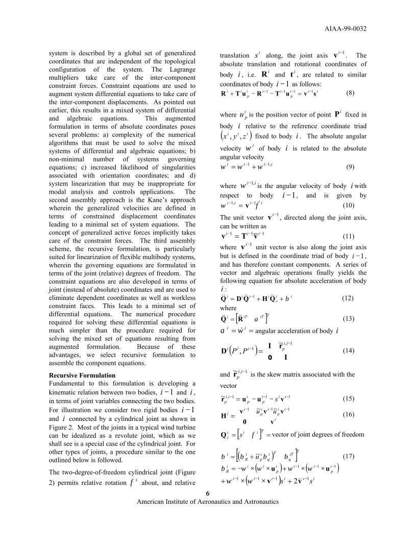
system is described by a global set of generalizedcoordinates that are independent of the topologicalconfiguration of the system. The Lagrangemultipliers take care of the inter-componentconstraint forces. Constraint equations are used toaugment system differential equations to take care ofthe inter-component displacements. As pointed outearlier, this results in a mixed system of differentialand algebraic equations. This augmentedformulation in terms of absolute coordinates posesseveral problems: a) complexity of the numericalalgorithms that must be used to solve the mixedsystems of differential and algebraic equations; b)non-minimal number of systems governingequations; c) increased likelihood of singularitiesassociated with orientation coordinates; and d)system linearization that may be inappropriate formodal analysis and controls applications. Thesecond assembly approach is the Kane’s approachwherein the generalized velocities are defined interms of constrained displacement coordinatesleading to a minimal set of system equations. Theconcept of generalized active forces implicitly takescare of the constraint forces. The third assemblyscheme, the recursive formulation, is particularlysuited for linearization of flexible multibody systems,wherein the governing equations are formulated interms of the joint (relative) degrees of freedom. Theconstraint equations are also developed in terms ofjoint (instead of absolute) coordinates and are used toeliminate dependent coordinates as well as worklessconstraint faces. This leads to a minimal set ofdifferential equations. The numerical procedurerequired for solving these differential equations ismuch simpler than the procedure required forsolving the mixed set of equations resulting fromaugmented formulation. Because of theseadvantages, we select recursive formulation toassemble the component equations.

Recursive FormulationFundamental to this formulation is developing akinematic relation between two bodies, 1−i and i ,in terms of joint variables connecting the two bodies.For illustration we consider two rigid bodies 1−iand i connected by a cylindrical joint as shown inFigure 2. Most of the joints in a typical wind turbinecan be idealized as a revolute joint, which as weshall see is a special case of the cylindrical joint. Forother types of joints, a procedure similar to the oneoutlined below is followed.

The two-degree-of-freedom cylindrical joint (Figure2) permits relative rotation iφ about, and relative

translation is along, the joint axis 1−iv . Theabsolute translation and rotational coordinates ofbody i , i.e. iR and it , are related to similarcoordinates of body 1−i as follows:

iiip

iiip

ii svuTRuTR 1111 −−−− =−−+ (8)

where ipu is the position vector of point iP fixed in

body i relative to the reference coordinate triad( )iii zyx ,, fixed to body i . The absolute angular

velocity iω of body i is related to the absoluteangular velocity

iiii ,11 −− += ωωω (9)

where ii ,1−ω is the angular velocity of body i withrespect to body 1−i , and is given by

iiii φω &1,1 −− = v (10)

The unit vector 1−iv , directed along the joint axis,can be written as

111 −−− = iii vTv (11)where 1−iv unit vector is also along the joint axisbut is defined in the coordinate triad of body 1−i ,and has therefore constant components. A series ofvector and algebraic operations finally yields thefollowing equation for absolute acceleration of bodyi :

iir

iiii β++= − QHQDQ &&&&&& 1 (12)where

[ ]TiTiTi αRQ &&&& = (13)

== ii ωα & angular acceleration of body i

( )

=

−−

IrI

D0

1,1

~,

iipiii PP (14)

and 1,~ −iipr is the skew matrix associated with the

vector111,~ −−− −−= iii

pip

iip s vuur (15)

=

−−−

i

iip

iip

ii uu

v0vvvH

111 ~~(16)

[ ] ==Tiii

r s φQ vector of joint degrees of freedom

( )[ ]TiTTiip

iR

i u θθ ββββ ~+= (17)

( ) ( )111 −−− ××+××−= ip

iiip

iiiR uu ωωωωβ

( ) iviiii ss 1111 2 −−−− +××+ vv &ωω

AIAA-99-0032


7

( ) iiii φωβθ&11 −− ×= v (18)

Note that the term of the matrices iD andiH depends on the joint type. Equations similar to

(12), representing two bodies interconnected by ajoint, are developed for spherical, universal,prismatic, resolute, and ball/sliding joints. Theresolute joint in fact can be considered as a specialcase of the cylindrical joint wherein translation is isheld constant, and the prismatic joint is also aspecial case of the cylindrical joint wherein therotation iφ is held constant.

If motion of the base body i is known, equation (12)can be used recursively to express absoluteacceleration of any body i in terms of the motion ofthe base body and the motion of all the joints thatconnect body i to the base body (the base body isusually the fixed ground). Use of Newton-Eulerequations in conjunction with equation (12) yields aminimal set of differential equations for each bodyexpressed in terms of the joint degrees of freedom.

In general, a multibody system, e.g., a wind turbine,consists of interconnected rigid and flexible bodies.Recursive relation (12) helps us to express themotion of reference frame of any body i in terms ofthe joint degrees of freedom and the motion of a baseframe that may be attached to a rigid body or aflexible body, e.g., the tower top. The equation ofmotion for each body thus is expressible in terms ofall the system joint degrees of freedom and all thesystem elastic degrees of freedom. These componentequations are simply collected and put in the matrixform:

NLE

J

NE

E

E

J

J

J

E

J

NE

E

E

J

J

J

E

J

NE

E

E

J

J

J

Fqq

K

KK

K

KK

qq

C

CC

C

CC

qq

M

MM

M

MM

=÷÷

+÷÷

+÷÷

MM&

&

MM&&

&&

MM

2

1

1

1

1

2

1

1

1

1

2

1

1

1

1

(19)where Jq and Eq represent the system joint andelastic degrees of freedom, respectively. Expressingthe system degrees of freedom as

[ ]TTE

TJ qqx = (20)

equation (19) can be put in the compact form:=++ KxxCxM &&& NLF (21)

A parallel effort is under way to extend Kane’sassembly scheme to include flexible components. Itappears that for the flexible components, a mixedformulation mentioned earlier would be required tomake assembly feasible. Should we succeed, we

would perform a comparative study and select anassembly approach that would be most advantageousin terms of automation, linearization, simplicity ofequations, and computational time.

LINEARIZATION

System equations in the implicit form, that aregenerally used by simulation codes, can be expressedas

0),,,,( =tfxxxg &&& (22)where x is the vector of system coordinates, f is thevector of applied, e.g., aerodynamic forces, and trepresents time. In the explicit form, the systemequations, resulting from the assembly of flexiblecomponent equations and rigid component equationsare expressed as

),,,,()()()( θwxxFxKxCxM tttt NL &&&& =++ (23)where w is the vector of wind velocity components,and θ is the vector of controls, e.g., pitch angles ofblades, which may be explicit functions of timeand/or the system coordinates x . )(tM , )(tC , and

)(tK are in general periodic functions of time. NLF isthe vector of constant and nonlinear forces.Expressing )(tx as a perturbation about the periodicsolution, i.e.

)()()( 0 ttt xxx ∆+= (24)equations (23) become

L&&

&&&&&&&

+∆

∂∂

+∆

∂∂

+=∆++∆++∆+ xxfx

xffxxKxxCxxM

xx 000000 )()()(

x

(25)or

),,(00

xxfxxfKx

xfCxM

x

&&&

&&&

tNLx

=∆÷÷

∂∂−+∆÷÷

∂∂−+∆

(26)

where 0f represents constant forces, e.g., time-invariant centrifugal forces, and NLf represents allnonlinear terms. Equation (26) represents the finalset of system linearized equations; the left-hand sidecomprises the linear part and the right-hand sidecomprises the nonlinear part. To compute modalfrequencies and vectors, we set the right-hand side tozero and use the Floquet approach.12,13 These modesthen may be used to transform equation (26) into themodal domain. Either these modal equations or thephysical-domain equations (26) can be transformedinto the first-order state-space format for use incontrols design.

AIAA-99-0032


8

CURRENT STATUS AND FUTURE WORK

We derived the wind turbine component equations,comprising both flexible and rigid parts. For therigid parts, we attempted three approaches:Lagrangian formulation based on global coordinatesand Lagrangian multipliers, recursive formulationusing joint coordinates, and Kane’s approach usingpartial speeds. This allows a wide choice ofassembly options. A library of joint constraints,based on Rodrigues parameters, has also beendeveloped that can be integrated into any of theassembly schemes. A scheme to symbolicallygenerate linearized equations has also beendeveloped. Figure 2 shows the organization of thecomputer code covering structural modeling. Thecode is being developed in a modular fashion toallow efficient data management, futuremodifications and expansions. Solid boxes indicatemodules that have been completely coded. Boxes indashed lines indicate modules under development.

Both the component and system would be validatedwith exact results, if available, and with other codes,e.g., the ADAMS code, using specific forcingfunctions and simulations. This will be followed bythe integration of structure code with unsteadyaerodynamics and dynamic induced inflow models instate-space formats. The resulting aeroelastic codewill be validated with ADAMS for typical windturbine configurations and specific simulations.Extensive results will be presented to demonstratethe ability of the code to compute operating modes,stability, and aeroelastic descriptive models indiverse formats.

ACKNOWLEDGEMENT

We wish to thank Prof. Dewey Hodges, GeorgiaInstitute of Technology, who provided technicalassistance on mixed formulation, automatedassembly of rigid body equations, and symboliclinearization. DOE supported this work undercontract number DE-AC36-83CH10093.

REFERENCES

1 Elliott, A.S. and Wright, A.D. (1994).“ADAMS/WT: An Industry-Specific InteractiveModeling Interface for Wind Turbine Analysis,”Wind Energy 1994, SED-Vol. 14, New York:American Society of Mechanical Engineers, pp. 111-122, January 1994.

2 Wilson, R.E., Freeman, L.N., Walker, S.N., andHarman, C.R. (1996). FAST Advanced DynamicsCode, Two-Bladed Teetered Hub Version 2.4 User’sManual, Final Report, National Renewable EnergyLaboratory, Golden Colorado, March 1996.3 Hansen, A.C. (1996). User’s Guide: YawDyn andAeroDyn for ADAMS, Version 9.6, NationalRenewable Energy Laboratory Report, Contract No.XAF-4-14076-02.4 Stuart, J., Wright, A., and Butterfield, C. (1996).“Considerations for an Integrated Wind TurbineControls Capability at the National WindTechnology Center: An Aileron Control Strategy forPower Regulation and Load Mitigation,”Proceedings of the American Wind EnergyAssociation, Windpower 1996, Denver, Colorado,June 23-27, 1996.5 Shabana, A.A. (1997). “Flexible MultibodyDynamics: Review of past and RecentDevelopments,” Journal of Multibody SystemDynamics 1, No. 2, pp 189-222.6 Schielen, W.O. (1982). “Dynamics of ComplexMultibody Systems,” SM Arch. 9, pp. 297-308.7 Bir, G., Chopra, I. (1990). “Development ofUMARC (University of Maryland Advanced RotorCode),” Proceedings of the 46th Annual Forum of theAmerican Helicopter Society, Washington, D.C.,May 1990.8 Bir, G. and Robinson, M. (1998). “Development ofWind Turbine Descriptive Models for AdvancedControl Design,” American Wind EnergyAssociation Conference, Windpower 1998,Bakersfield, California, April 27-May 1, 1998.9 Wehage, R.A. (1980). “Generalized CoordinatePartitioning in Dynamic Analysis of MechanicalSystems,” Ph.D. dissertation, University of Iowa,Iowa City.10 Kane, T.R. and Levinson, D.A. (1985). Dynamics:Theory and Applications, McGraw-Hill, Inc.11 Shabana, A.A. (1998). Dynamics of MultibodySystems, Cambridge University Press.12 Johnson, W. (1980). Helicopter Theory, PrincetonUniversity Press.13 Bir, G. and Stol, K. (1999). “Operating Modes of aTwo-Bladed Wind Turbine,” Proceedings of the

AIAA-99-0032


9

IMAC-XVII Conference, Hyatt Orlando, Kissimmee,Florida, February 8-11, 1999.14 Sivaneri, N.T. and Chopra, I. (1984). “FiniteElement Analysis for Bearinless Rotor BladeAeroelasticity,” Journal of the American HelicopterSociety, Vol. 29, No.2, April 1984.15 Hodges, D.H. (1987). “Finite Rotation andNonlinear Beam Kinematics,” Vertica, Vol. 11,No.1/2, pp. 297-307.

AIAA-99-0032


10

il

ix

3eu 3φ 4eu

1

1

1

1

1

1

'

'

φwwvvue

2

2

2

2

2

2

'

'

φ

wwvvu e

Figure 1. Fifteen degrees of freedom finite element used to discretize the flexible beam

Figure 2. Relative motion of body i with respect to body 1−i .

AIAA-99-0032


11

Figure 3. Major modules of the structures code (solid lines identify completed modules, dashed lines identifymodules under development)

INPUTPROCESSOR

EIGENSOLVERLINEARIZERSYSTEMEOM

COMPONENTS EOM

RIGIDPARTSNACELLE

BED-FRAMEGENERATOR

FLEXIBLEPARTSBLADESTOWERSHAFT

PHYSICALMODEL

ASSEMBLY

MAIN

INPUT

MBCTRANS

BEAMELEMENTLIBRARY

CONSTRAINTSLIBRARY

FLOQUET

STATE-SPACEMODEL

MODAL-DOMAINMODEL

MODES

code development for control design applications phase … · nrel/cp-500-25792 code development...

Documents