Cockroaches and Thylacines: The Hazards of Species Extinction

Christopher G. Small, University of Waterloo(joint with Sheena Zhang & Grace Chiu)

Dedicated to

Eric Rowland Guiler

(1922—2008)

In this talk, I shall examine the problems of species extinction at the macro- and micro-levels. At the macro-level, I shall consider the

statistics of extinction in the fossil record. At the micro-level, I shall try to extract a

few facts from the limited data we have about the thylacine population in the late nineteenth and early twentieth centuries.

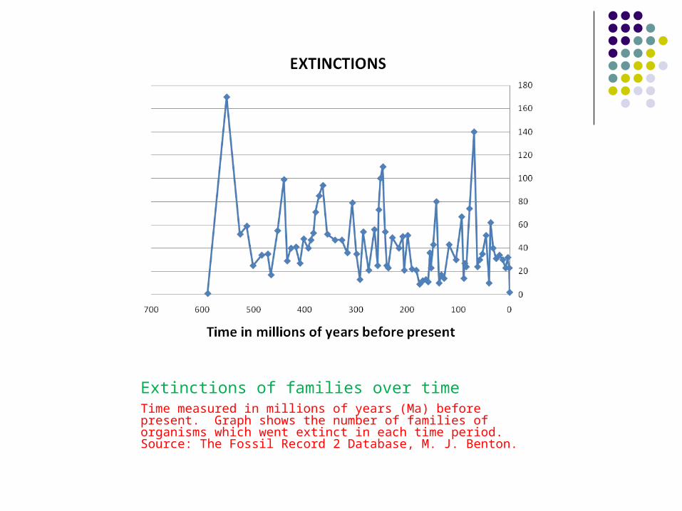
Extinctions of families over time Time measured in millions of years (Ma) before present. Graph shows the number of families of organisms which went extinct in each time period. Source: The Fossil Record 2 Database, M. J. Benton.

Extinctions (EXT) against time interval (INT):

Taxonomic families have become extinct at a rate of 5.858 families/Ma over the last 550 MY.

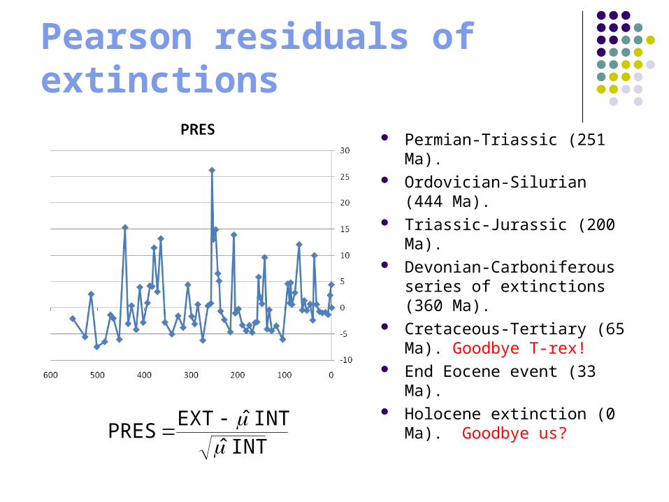
Pearson residuals of extinctions

Permian-Triassic (251 Ma).

Ordovician-Silurian (444 Ma).

Triassic-Jurassic (200 Ma). Devonian-Carboniferous

series of extinctions (360 Ma).

Cretaceous-Tertiary (65 Ma). Goodbye T-rex!

End Eocene event (33 Ma).

Holocene extinction (0 Ma). Goodbye us?

INTˆ

INTˆEXTPRES

Mass extinctions: standard?

Variation in size of extinctions far exceeds “background noise.” I.e., extinctions of taxa are clustered not independent.

Mass extinctions are extreme but not exceptional. (David Raup, 1991).

Mass extinctions are both extreme and exceptional (Richard Bambach & Andrew Knoll, 2001).

Extinctions have occurred at a fairly constant rate on average over time despite occasional mass extinctions.

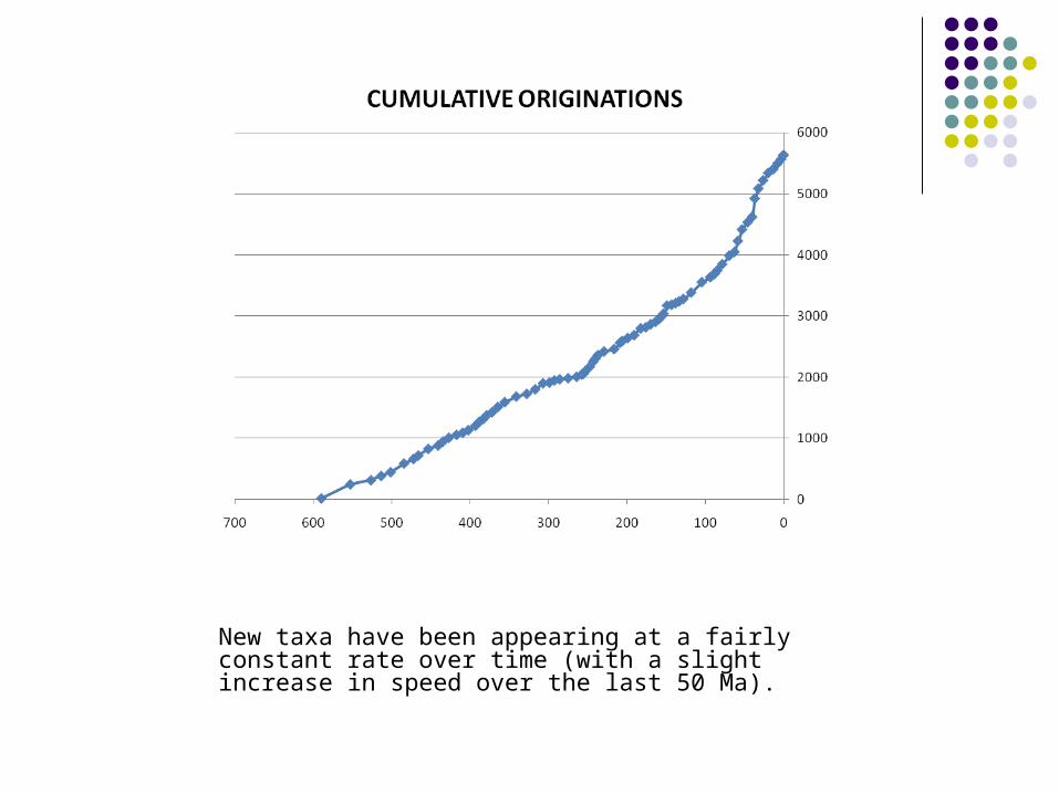
New taxa have been appearing at a fairly constant rate over time (with a slight increase in speed over the last 50 Ma).

However ……………..

Diversity over time (Ma)The diversity of taxa (in this case families) at any given time has been steadily increasing (with a slight drop at the end of the Palaeozoic).

The hazards of extinction

The statistical approach to studying these extinctions is to treat each species or family as subject to an ongoing hazard of extinction.

This hazard is quantified by means of a hazard function whose value can change over time.

The probability of extinction will depend upon the value of the hazard integrated over time.

Hazards of extinction

Let )(t denote the hazard f unction f or extinction of a

randomly chosen taxon (species, f amily, phylum …) at

time t. That is, dtt)( is the probability of extinction

of the taxon in a time interval of length dt given its

survival up to time t .

For example, if the extinction rate is constant over

time, then )(t f or all t, and the probability of

extinction by time tt of a species extant at time t

is

te 1 .

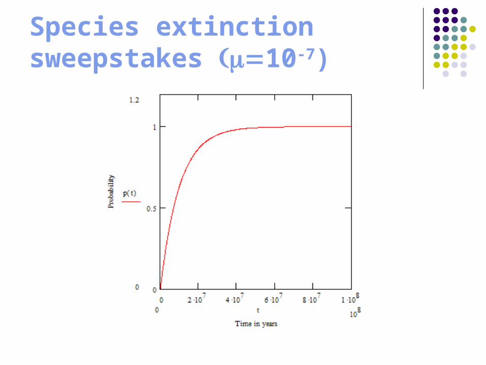
Species extinction sweepstakes 10-7)

Winners and losers

Winner? (> 108 years) Loser? (4 x 106 years)

Estimating nonconstant hazard functions To estimate the hazard function, we would like to

observe extinctions in the fossil record and when they happened.

So we would like to know the precise number of taxa that are extant at different times.

Unfortunately, this is difficult: counts are binned into time periods, dating of individual fossils is uncertain pseudoextinction, Lazarus taxa, Elvis taxa.

At best we use proxy variables at any time we can determine the taxa that appear

before and after that time.

STAGE DURATION MIDPOINT ORIGINS EXTINCTIONS DIVERSITY

VENDIAN 40 590 4 1 16

CAERFAI 34 555.5 230 170 245

ST DAVID'S 19 527 68 52 143

MERIONETH 7 513.6 70 59 161

TREMADOC 17 501.5 62 25 164

ARENIG 17 484.5 142 34 281

LLANVIRN 7.5 472.3 74 35 321

LLANDEILO 4.5 466.3 57 17 343

CARADOC 21 453.5 108 55 434

ASHGILL 4 441 54 99 433

LLANDOVERY 8.5 434.7 66 29 400

WENLOCK 6.5 427.2 63 40 434

Let )(tN be the number of taxa that are extant a

time t . Proxy variables will henceforth be represented

by using a tilde.

A proxy f or )(tN is )(~ tN : the number of taxa

that appear in the f ossil record both before and

af ter time t . Let

)(~)(~)(~ ttNtNtN

)(~ln)(~ln)(~ln ttNtNtN

Let )(~ tE be the cumulative number of taxa that

appear before time t but not af ter time t . Defi ne

)(~ tE similarly.

Define )(~tO be the number of taxa that appear

af ter time t but not before t , and )(~tO similarly.

Generalized Birth and Death Process

Assumptions (D. Stoyan, 1980):

Let )(t be the hazard f unction f or a

taxon to become extinct at time t .

Similarly, )()()( tttt

Let )(t be the rate of speciation of a

given taxon into new taxa at time t .

Similarly, )()()( tttt .

Given all the information about extant

taxa at time t , the expected number of

extinctions between t and tt is

ds

dxxxe

tt

ttNstE

st

)()(

)()()(

E.

Given all the information about extant

taxa at time t , the expected number of

originations between t and tt is

ds

dxxxe

tt

ttNstO

st

)()(

)()()(

E.

.

When t is small these integrals

reduce to

)()(1

)]()([)()()(

tt

ttte

tNttE

E

and

)()(1

)]()([)()()(

tt

ttte

tNttO

E

So estimators f or and are f ound by

substituting proxies and solving

)(ˆ)(ˆ1

)](ˆ)(ˆ[)(~)(ˆ)(~

tt

ttte

tNttE

and

)(ˆ)(ˆ1

)](ˆ)(ˆ[)(~)(ˆ)(

~tt

ttte

tNttO

These simultaneous equations have

solutions

ttN

tNtE

t

)(~ln

)(~)(~

)(̂

and

ttN

tNtO

t

)(~ln

)(~)(

~)(̂

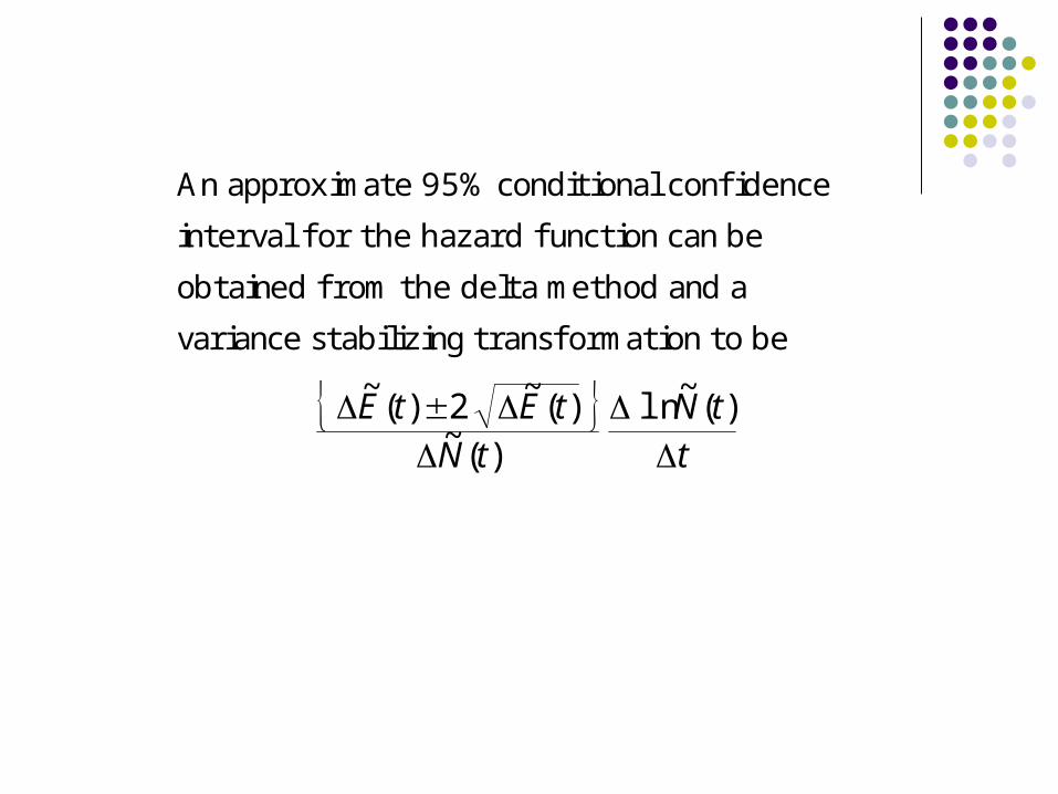
An approximate 95% conditional confi dence

interval f or the hazard f unction can be

obtained f rom the delta method and a

variance stabilizing transformation to be

ttN

tN

tEtE

)(~ln

)(~)(~2)(~

Comments

Most extinctions are “mass extinctions.” The Generalised BD model is useful for hazards, but does not fit other aspects of

data well. Models for extinctions must explain the homogeneity of extinctions and

originations in the face of increasing diversity of taxa. Research may be concentrating too much on taxa and not enough on ecological

niches (D. H. Erwin, 2006).

We should be modelling hazards and not simply fitting them. Current work is investigating modelling the extinction rate as a nonnegative

strongly stationary process. Without modelling there are no null hypotheses: 26 Ma cycles of extinction?

(Raup and Sepkoski,1984). Statistical artefact? (Stigler and Wagner).

The error analysis of proxy variables is nontrivial. It is formally equivalent to the problem of estimating the support of a distribution. C. Marshall (1994), but more work necessary!

Decline of the thylacine

Possible sources of thylacine decline:

Hunting and trapping (the latter for zoos worldwide).

Destruction of habitat. Competition with wild dogs. Disease (esp. reports of a “distemper-

like” disease, 1910).

0

20

40

60

80

100

120

140

160

180

1888

1889

1890

1891

1892

1893

1894

1895

1896

1897

1898

1899

1900

1901

1902

1903

1904

1905

1906

0

2

4

6

8

10

12

14

16

18

20

TasmaniaWoolnorth

Thylacines presented for govt. bounty & thylacines killed at Woolnorth

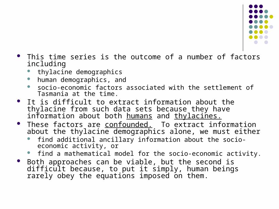
This time series is the outcome of a number of factors including thylacine demographics human demographics, and socio-economic factors associated with the settlement of Tasmania

at the time. It is difficult to extract information about the thylacine from

such data sets because they have information about both humans and thylacines.

These factors are confounded. To extract information about the thylacine demographics alone, we must either find additional ancillary information about the socio-economic

activity, or find a mathematical model for the socio-economic activity.

Both approaches can be viable, but the second is difficult because, to put it simply, human beings rarely obey the equations imposed on them.

Van Diemen’s Land Company at Woolnorth

Records at VDL Company, Woolnorth (E. Guiler, 1985)

1899 26 Aug. Tom went to the Mount to look after a tiger with his dogs.

2 Nov. Sent some men to hunt tiger out of Studland Bay run.

11 Nov. All hands in a.m. hunting a tiger out of the Forest. Set snares for a tiger on Saltwater Creek fence.

1890 6 Feb. Tracks seen in Forest.

27 May Chasing tiger in the Forest.

17 July Tiger at Studland Bay, at the Knolls.

1891 1 Aug. Laid poison at Harcus for hunters’ dogs.

1892 26 Aug. Two men to Studland Bay to shift tiger.

1893 No comments.

Records at VDL Company, Woolnorth (continued)

1898 20 Feb. One tiger caught, no locality given.

20 July One tiger caught, McCabe’s Paddock

31 Dec. Snaring in the Forest.

1899 3 July Saw two tigers at Swan Bay.

6 July Caught two tigers in Forest and Three Sticks

22 July Tiger scaring on Three Sticks and Studland Bay

23 Nov. One tiger caught, probably at the Mount.

1900 24 Jan. One tiger caught, locality not stated.

8 Feb. Tiger scaring at Three Sticks

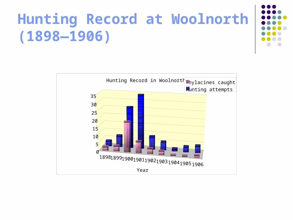
Hunting Record at Woolnorth (1898—1906)

189818991900190119021903190419051906

0

5

10

15

20

25

30

35

Year

Hunting Record in Woolnorth Thylacines caughtHunting attempts

We model the number of potential encounters of thylacines in year t as binomial with parameters )(tn and p , where )(tn is

the (unknown) number of thylacines in the area at time t and p

is the (unknown) probability of killing per individual. Let )(th be

the probability that a thylacine hunt at time t is “successful.”

.1

}0)),((BinPr{1

}0)),((BinPr{)(

)(tnpe

ptn

ptnth

Theref ore, )(tn will be

p

thtn

)](1[ln)(

.

Suppose we model the rate of decline of )(tn as

)()(

tndt

tndE

E ,

which implies that 0)(ln Cttn . Then

.error

errorln)](1[lnln 0

Ct

pCtth

Therefore, we model using the regression equation:

jjj Ctth )](1[lnln

which can be fi t by usual least square methods.

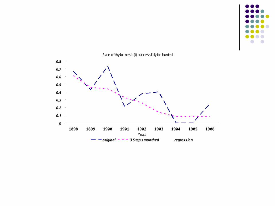
Rate of thylacines h(t) successfully be hunted

0

0.1

0.2

0.3

0.4

0.5

0.6

0.7

0.8

1898 1899 1900 1901 1902 1903 1904 1905 1906Year

original 3 Step smoothed regression

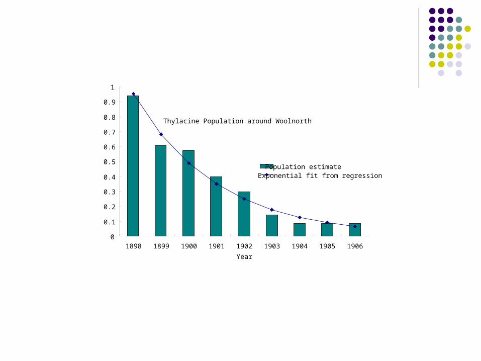
Thylacine Population around Woolnorth

0

0.1

0.2

0.3

0.4

0.5

0.6

0.7

0.8

0.9

1

1898 1899 1900 1901 1902 1903 1904 1905 1906

Year

Population estimate Exponential fit from regression

Comments

The data suggest that by the beginning of the twentieth century the decline in the thylacine population was substantial.

While a “distemper-like” disease may have contributed to thylacine decline, the evidence is that the thylacine was disappearing before this.

Habitat, dogs and hunting are the main factors to be considered.

References Bambach, R. K. & Knoll, H. (2001). “Is there a separate class of `mass

extinctions?’” GSA Annual Meeting, 5—8 November 2001. Erwin, Douglas H. (2006). Extinction: How Life on Earth Nearly Ended

250 Million Years Ago. Princeton University. Guiler, Eric R. (1985). Thylacine: The Tragedy of the Tasmanian

Tiger, Oxford University. Marshall, C. R. (1994). “Confidence intervals on stratigraphic ranges:

partial relaxation of the assumption of randomly distributed fossil horizons.” Paleobiology 20, 459—469.

Raup, D. M. (1991). Extinction: Bad Genes or Bad Luck? Norton. Raup, D. M. & Sepkoski, J. J. Jr. (1984). “Periodicity of extinction in the

geologic past.” Proc. Nat. Acad. Sci. USA 81, 801—805. Stigler, S. M. & Wagner, M. J. (1987). “A substantial bias in

nonparametric tests for periodicity in geophysical data.” Science 13, 940—945.

Stoyan, D. (1980). “Estimation of transition rates of inhomogeneous birth-death processes with a paleontological application.” Elektronische Informationsverabeitung u. Kybernetic 16, 647—649.