Coastal Water Quality Monitoringin Shrimp Farming Areas:

An Example from Honduras

CCOOAASSTTAALL WWAATTEERR QQUUAALLIITTYY MMOONNIITTOORRIINNGG IINN SSHHRRIIMMPP FFAARRMMIINNGG AARREEAASS::

AANN EEXXAAMMPPLLEE FFRROOMM HHOONNDDUURRAASS

CCllaauuddee EE.. BBooyydd aanndd

BBaarrtthhoolloommeeww WW.. GGrreeeenn

DDeeppaarrttmmeenntt ooff FFiisshheerriieess aanndd AAlllliieedd AAqquuaaccuullttuurreess AAuubbuurrnn UUnniivveerrssiittyy,,

AAllaabbaammaa 3366884499,, UUSSAA

AA RReeppoorrtt PPrreeppaarreedd ffoorr tthhee

WWoorrlldd BBaannkk,, NNeettwwoorrkk ooff AAqquuaaccuullttuurree CCeennttrreess iinn AAssiiaa--PPaacciiffiicc,, WWoorrlldd WWiillddlliiffee FFuunndd aanndd FFoooodd aanndd AAggrriiccuullttuurree OOrrggaanniizzaattiioonn ooff tthhee UUnniitteedd NNaattiioonnss

CCoonnssoorrttiiuumm PPrrooggrraamm oonn SShhrriimmpp FFaarrmmiinngg aanndd tthhee EEnnvviirroonnmmeenntt

ii

The findings, interpretations, and conclusions expressed in this paper are entirely those of the co-editors and contributors and should not be attributed in any manner to the World Bank, to its affiliated organizations that comprise the World Bank Group, or to any of their Executive Directors or the countries they represent, or to the World Wildlife Fund (WWF), or the Network of Aquaculture Centres in Asia-Pacific (NACA) or the Food and Agriculture Organization of the United Nations (FAO). The World Bank, World Wildlife Fund (WWF), the Network of Aquaculture Centres in Asia-Pacific (NACA) and Food and Agriculture Organization of the United Nations (FAO) do not guarantee the accuracy of the data included in this report and accept no responsibility whatsoever for any consequence of their use. The boundaries, designations, colors, denominations, and other information shown on any map in this volume do not imply on the part of the World Bank Group, World Wildlife Fund (WWF), the Network of Aquaculture Centres in Asia-Pacific (NACA) or Food and Agriculture Organization of the United Nations (FAO) any judgment or expression of any opinion on the legal status of any territory or the endorsement or acceptance of boundaries.

COPYRIGHT AND OTHER INTELLECTUAL PROPERTY RIGHTS, Food and Agriculture Organization of the United Nations (FAO), the World Bank Group, World Wildlife Fund (WWF), and the Network of Aquaculture Centres in Asia-Pacific (NACA), 2002.

All copyright and intellectual property rights reserved. No part of this publication may be reproduced, altered, stored on a retrieval system, or transmitted in any form or by any means without prior permission of the Food and Agriculture Organization of the United Nations (FAO), the World Bank Group, World Wildlife Fund (WWF) and the Network of Aquaculture Centres in Asia-Pacific (NACA), except in the cases of copies intended for security back-ups or for internal uses (i.e., not for distribution, with or without a fee, to third parties) of the World Bank Group, FAO, WWF or NACA. Information contained in this publication may, however, be used freely provided that the World Bank Group, FAO, WWF and NACA be cited jointly as the source.

iii

Preparation of this document

The research reported in this paper was prepared under the World Bank/NACA/WWF/FAO Consortium Program on Shrimp Farming and the Environment. Due to the strong interest globally in shrimp farming and issues that have arisen from its development, the consortium program was initiated to analyze and share experiences on the better management of shrimp aquaculture in coastal areas. It is based on the recommendations of the FAO Bangkok Technical Consultation on Policies for Sustainable Shrimp Culture1, a World Bank review on Shrimp Farming and the Environment2, and an April 1999 meeting on shrimp management practices hosted by NACA and WWF in Bangkok, Thailand. The objectives of the consortium program are: (a) Generate a better understanding of key issues involved in sustainable shrimp aquaculture; (b) Encourage a debate and discussion around these issues that leads to consensus among stakeholders regarding key issues; (c) Identify better management strategies for sustainable shrimp aquaculture; (d) Evaluate the cost for adoption of such strategies as well as other potential barriers to their adoption; (e) Create a framework to review and evaluate successes and failures in sustainable shrimp aquaculture which can inform policy debate on management strategies for sustainable shrimp aquaculture; and (f) Identify future development activities and assistance required for the implementation of better management strategies that would support the development of a more sustainable shrimp culture industry. This paper represents one of the case studies from the Consortium Program. The program was initiated in August 1999 and comprises complementary case studies on different aspects of shrimp aquaculture. The case studies provide wide geographical coverage of major shrimp producing countries in Asia and Latin America, as well as Africa, and studies and reviews of a global nature. The subject matter is broad, from farm level management practice, poverty issues, integration of shrimp aquaculture into coastal area management, shrimp health management and policy and legal issues. The case studies together provide an unique and important insight into the global status of shrimp aquaculture and management practices. The reports from the Consortium Program are available as web versions (http://www.enaca.org/shrimp) or in a limited number of hard copies. The funding for the Consortium Program is provided by the World Bank-Netherlands Partnership Program, World Wildlife Fund (WWF), the Network of Aquaculture Centres in Asia-Pacific (NACA) and Food and Agriculture Organization of the United Nations (FAO). The financial assistance of the Netherlands Government, MacArthur and AVINA Foundations in supporting the work are also gratefully acknowledged. Correspondence: Claude Boyd, Email: ceboyd@acesag.auburn.edu Reference: Boyd, C. E. and B.W. Green. 2002. Coastal Water Quality Monitoring in Shrimp Farming Areas, An Example from Honduras. Report prepared under the World Bank, NACA, WWF and FAO Consortium Program on Shrimp Farming and the Environment. Work in Progress for Public Discussion. Published by the Consortium. 29 pages.

1 FAO. 1998. Report of the Bangkok FAO Technical Consultation on Policies for Sustainable Shrimp Culture. Bangkok, Thailand, 8-11 December 1997. FAO Fisheries Report No. 572. Rome. 31 p. 2 World Bank. 1998. Report on Shrimp Farming and the Environment – Can Shrimp Farming be Undertaken Sustainability? A Discussion Paper designed to assist in the development of Sustainable Shrimp Aquaculture. World Bank. Draft.

iv

Abstract

Various substances in shrimp farm ponds can contaminate waters, including nutrients (nitrogen and phosphorus), metabolic wastes, antibiotics, or other medicines to protect shrimp, and suspended soil particles from erosion. This report discusses ways to monitor these aspects of water quality, which is important from two standpoints for shrimp farmers. Incoming water used top supply shrimp ponds must be healthful and free of toxins to protect the growing shrimp, and effluent must be clean enough to avoid harming aquatic ecosystems downstream, and in many places to meet water quality standards. The requirements and costs of setting up and operating a water quality analysis lab are provided, and the report describes methods of sampling and analyzing water samples. Key aspects of lab operations, including testing the accuracy and precision of analytical procedures, and using quality control, range control, and means control charts are discussed, with numerical examples. The report recommends procedures for recording data and keeping accurate, organized records. The second part of the report covers a water quality monitoring project in the Gulf of Fonseca, where shrimp aquaculture in Honduras is centered. The research—collaborative work among universities, private sector aquaculturists (through the industry organization ANDAH), and government offices—has continued since 1993. Regular sampling of estuary water (near where pumps discharge incoming water into farm supply canal) is conducted by shrimp farmers and analyzed in the laboratory set up to anchor the program. Research results are shared with shrimp farms in order to maintain participation and encourage farmers to become more aware of the interaction between shrimp farming and the environment. Although shrimp farm area has grown substantially since 1993, and production has grown some, no increase in eutrophication of estuaries in southern Honduras has been found over this period. (Riverine estuary water quality changes notably by season, with nutrient concentrations higher in the dry season. Similar though much less pronounced changed occur in embayments.) Seeking to reduce the amount of nutrients entering estuaries, aquaculture farms have reduced their feed and fertilizer input into shrimp ponds, and tried using lower protein feeds. Salinity can also drop sharply in estuaries during the rainy season, from freshwater runoff. The report concludes that a strong industry association and support from government are critical to implementing a successful water quality monitoring program and, ultimately, to maintaining aquaculture sustainable. ANDAH promotes effective regulation to protect the country’s natural resources. The monitoring program is also supported by effective research and communication of results.

v

Content

ABSTRACT ............................................................................................................................................... IV

ABBREVIATION AND ACRONYMS ...................................................................................................VI

INTRODUCTION....................................................................................................................................... 1

WATER QUALITY MONOTORING ...................................................................................................... 2

VARIABLES................................................................................................................................................ 3

ANALYTICAL TECHNIQUES ................................................................................................................ 5

SAMPLING ................................................................................................................................................. 6 LOCATIONS................................................................................................................................................................. 6 SAMPLING FREQUENCY .............................................................................................................................................. 6 TIME OF SAMPLING..................................................................................................................................................... 6 OTHER ASPECTS OF SAMPLING ................................................................................................................................... 7

FIELD AND LABORATORY REQUIREMENTS.................................................................................. 7

RELIABILITY OF DATA ......................................................................................................................... 8

ACCURACY AND PRECISION ............................................................................................................... 8

QUALITY CONTROL ............................................................................................................................... 8 STANDARD OPERATING PROCEDURES ........................................................................................................................ 8 PRECISION AND ACCURACY CHECKS .......................................................................................................................... 8 QUALITY CONTROL CHARTS..................................................................................................................................... 10 CONTROL CHARTS .................................................................................................................................................... 10 MEANS CONTROL CHART ......................................................................................................................................... 12

RECORD KEEPING AND DATA ANALYSIS ..................................................................................... 14

COSTS........................................................................................................................................................ 15

PERFORMANCE INDICATORS FOR MONITORING PROGRAMS............................................. 16

EFFECTS OF EFFLUENTS.................................................................................................................... 16

ESTUARINE MONITORING: AN EXAMPLE FROM HONDURAS ............................................... 17 PROJECT DESIGN AND IMPLEMENTATION ................................................................................................................. 18 SAMPLING AND ANALYSES ....................................................................................................................................... 21

RESULTS................................................................................................................................................... 22

FACTORS FOR SUCCES........................................................................................................................ 26

BIBLIOGRAPHY ..................................................................................................................................... 28

vi

Abbreviation and Acronyms

ANDAH Honduran National Association of Aquaculturists ANZECC Australian and New Zealand Environment and Conservation Council APHA American Public Health Association BMPs Better or Best Management Practices BOD Biochemical Oxygen Demand CL Control Limit cm Centimeters DIGEPESCA General Directorate of Fisheries and Aquaculture EAP Panamanian Agricultural School FPX Federation of Producers and Exporters of Honduras ha Hectare ICAAE International Center for Aquaculture and Aquatic Environments kg Kilogram l Liter m Meter MAL Ministry of Agriculture and Livestock mg Miligram N Number PD/A CRSP Pond Dynamics/Aquaculture Collaborative Research Support Program PPT Parts Per Thousand R Range s Second SOPs Standard Operating Procedures TSS Total Suspended Solids US AID United States Agency for International Development US$ American dollars WL Warning Limit

1

Introduction

Shrimp farming is a common activity in coastal zones of many tropical and subtropical nations. Shrimp farms are constructed near sources of brackish water or seawater, and ponds for shrimp culture are filled and maintained by pumping water from these sources. Fertilizers and feeds are both applied to ponds to promote shrimp growth. Nitrogen and phosphorus in fertilizers enhance phytoplankton production, enlarging the base of the food chain for shrimp. Feed is consumed directly by shrimp, often creating much greater production than with fertilizers alone. However, uneaten feed, feces, and other metabolic wastes increase nutrient concentrations in pond water, also stimulating phytoplankton growth. Effluents from shrimp ponds typically are enriched with nutrients, especially nitrogen and phosphorus, and they have high concentrations of particulate organic matter resulting from live plankton and decaying plankton. Waters in shrimp ponds usually are eutrophic, and the degree of eutrophication increases as shrimp production levels increase. In semi-intensive shrimp farming, water is flushed through ponds to reduce concentrations of nutrients, phytoplankton, ammonia, and other potentially toxic metabolites, as well as organic matter. In intensive shrimp farming, mechanical aeration is used to prevent low dissolved oxygen concentrations, but water exchange (flushing) is also commonly used. Water flushed from ponds enters coastal ecosystems, where it can cause eutrophication. Various chemicals may be applied to shrimp ponds in efforts to improve water quality or combat shrimp diseases. These chemicals include liming materials, zeolite, chlorine, formalin, insecticides, and antibiotics or other drugs. Normally, natural processes within culture ponds deactivate these chemicals, but there is opportunity for their release into coastal waters (Boyd and Massaut 1999). The land surface is disturbed when shrimp farms are constructed. Surface soils exposed by pond embankments, canals, roads, and other earthen infrastructure are often saline and do not revegetate naturally. Erosion occurs and runoff from exposed, bare soil has high concentrations of suspended solids (soil particles). Soil particles are also suspended by water flowing through canals and water currents generated by wind action and mechanical aeration. Another major source of suspended solids is the draining of ponds during shrimp harvests. The outflowing water suspends sediment from pond bottoms, and effluents during the final phase of harvest are especially high in suspended solids (Boyd and Tucker 1992). Shrimp farms thus represent potential sources of nutrient pollution, organic enrichment, turbidity and sedimentation in coastal waters. Some possibility exists for release of potentially toxic or bioaccumulative substances in pond effluents, as well. Shrimp farm effluents contain high concentrations of dissolved salts from brackish water and seawater used to fill ponds, exchange water, and maintain water levels, so discharge of effluents into freshwater areas can cause salinization. Obviously, indiscriminate discharge of shrimp pond effluents can cause eutrophication, excessive turbidity, sedimentation, toxicity, and salinization of aquatic habitats. These negative impacts can reduce the value of coastal ecosystems for other uses and adversely affect the native flora and fauna. Therefore, it is important to reduce the volume and enhance the quality of shrimp pond effluents and minimize the possibility for adverse environmental impacts. It should be possible to greatly reduce these impacts through better practices, such as more efficient use of feeds and fertilizers, reduction in water exchange, erosion control, restricted chemical use, installing sedimentation basins, and additional measures discussed in other case studies. Nevertheless, it is impossible, at least in the near future, to eliminate completely discharge from shrimp ponds. Therefore, monitoring programs to assess shrimp farm effluents are needed. These monitoring programs can determine whether better management practices (BMPs) installed or implemented on shrimp farms actually improve effluent quality and reduce pollutant loads. Monitoring can also indicate whether coastal water quality is deteriorating as a result of shrimp farming and other activities in an area. Monitoring

2

water quality should be an integral part of environmental management programs to reduce or prevent negative impacts of shrimp farming. This case study discusses the technical aspects of water quality monitoring programs for shrimp farming, and provides a review of a water quality monitoring program that has been ongoing for several years in the shrimp farming area of Honduras (Figure 1).

Figure 1. Map of Gulf of Fonseca and shrimp farming in southern Honduras. Water Quality Monotoring

The purpose of monitoring is to determine water quality measures at a point in time in a specific area and to determine whether changes in water quality occur after that point. It would be desirable to start a water quality monitoring program before the human activity of concern is initiated, in order to determine baseline values absent that activity. With shrimp farming, this will often be impossible because shrimp farms already have been operating in many areas for years. In this case, it is necessary to use the current condition as a beginning point, and from this reference, determine whether water quality deteriorates in the future. Or it may be possible to find a nearby area without shrimp farming to use for comparison. Shrimp farming is seldom the only activity influencing water quality in an area, so changes in water quality observed during a monitoring program may not result from shrimp farming alone. A water quality monitoring program for shrimp farming should take into account other possible sources of pollution and evaluate the amounts originating from all sources.

3

Most people consider monitoring programs useful strictly for evaluating the influence of some human activity on environmental quality. In the case of shrimp farming, however, maintaining good water quality is also essential for shrimp production. If source water for shrimp farms is appreciably degraded by pollution, impaired water quality in culture ponds will make producing shrimp much more difficult. Such environmental stress results in less efficient growth of the shrimp, greater susceptibility to disease, and higher mortality rates. Thus, it is important for shrimp farms to have information on the status of source water quality and to know whether its quality is deteriorating. In spite of the many problems associated with evaluating the actual influence of shrimp farming on coastal water quality, monitoring of farm effluent can be a powerful tool. In addition to providing information on the state of coastal water quality, effluent monitoring can demonstrate the effects of changes in production practices and management inputs on pollutant loads in effluents. Adoption of best management practices (BMPs) may be the major method for reducing the negative environmental impacts of shrimp farming. Monitoring of farm effluents will allow an objective evaluation of the benefits of BMPs. In the future, greater emphasis will be given to monitoring water quality in shrimp farm effluents and in coastal waters near shrimp farms. These monitoring programs will most probably be designed and conducted by individuals or organizations with relatively little experience in water quality monitoring. Many of these programs are likely to be technically flawed and justifiably subject to criticism. It is important, therefore, to provide a discussion of the critical factors in the design and operation of water quality monitoring programs for assessing shrimp farm effluents and their effects on coastal water quality. Variables

A great number of water quality variables could be measured, but for practicality, only the important variables should be measured. The variables of most importance in shrimp farming effluents are those most likely to cause deterioration of conditions in coastal ecosystems (Table 1).

4

Table 1. Guidelines for water quality monitoring programs for shrimp farm effluents and coastal waters. Modified from Australian and New Zealand Environmental and Conservation Council 1992.

Variable

Reason for measuring

Guidelines for protecting aquatic ecosystems

Water temperature Has marked influence on chemical and biological processes

Less than 2oC change

Dissolved oxygen Essential for aerobic aquatic life Not less than 5 to 6 mg/l

PH Influences chemical and biological processes

6.0 to 9.0

Total ammonia nitrogen Plant nutrient and potential toxin; indicator of pollution

Should not exceed 3 mg/l in effluents.

Nitrate nitrogen Potential toxin Should not exceed 0.005mg/l in coastal waters.

Total phosphorus Source of soluble inorganic phosphorus for plants

Concentrations of 0.001 to 0.1 mg/l in coastal waters can cause plankton blooms.

Total nitrogen Source of dissolved inorganic nitrogen for plants

Concentrations of 0.1 to 0.75 mg/l in coastal waters can cause plankton blooms. Should not exceed 10 mg/l in effluents.

Chlorophyll a Indicator of phytoplankton abundance and degree of eutrophication

Concentrations above 1 to 10 µg/L indicate eutrophication in coastal waters.

Total suspended solids Indicator of suspended soil particles or suspended organic matter.

Should not change by more than 10% of seasonal mean in coastal waters.

Biochemical oxygen demand Indicator of organic pollution Should not depress dissolved oxygen concentrations below 5 or 6 mg/l.

Salinity Can cause salinization Should not increase above 0.5 ppt in fresh water. No limit recommended for marine or brackish waters.

Secchi disk visibility Index of water clarity or turbidity Should not change by more than 10% of seasonal mean in coastal waters.

Note: The guidelines for protecting aquatic ecosystems are not effluent limits; they apply to the receiving water body outside the mixing zone. These limits do not apply within the mixing zone. Effluent concentration limits must be established so that the above limits are maintained within the receiving water outside of the mixing zone. A number of other variables (e.g., nitrate-nitrogen, soluble reactive phosphorus, chemical oxygen demand, particulate organic matter, volatile solids, oil and grease, settleable solids, and turbidity), could be included, but we do not think that these analyses are necessary. It is preferable to select a few important indicators that can be reliably measured and interpreted rather than to analyze a wide range of variables, some of which cannot be measured reliably or easily interpreted. Measurements of nitrate-nitrogen and soluble reactive phosphorus do not appreciably supplement total nitrogen and total phosphorus data for evaluating nutrient pollution. Chemical oxygen demand is difficult to measure in brackish water or seawater because of chloride interference. Biochemical oxygen demand provides adequate information on the potential of effluents for organic enrichment. It is also much easier to interpret biochemical oxygen demand data than data on chemical oxygen demand, particulate organic matter, volatile solids, and other measures of organic enrichment. Oil and grease generally result from fuel or lubricant leaks into the culture system. Oil and grease can be prevented from entering systems through use of BMPs, so that gathering data on oil and grease, which are difficult to interpret, would not be required. Data on settleable solids and turbidity only supplement total suspended solids information. Of course, turbidity is easy to measure, and some may want to substitute turbidity for total suspended solids for analytical convenience.

5

As pointed out earlier, many chemical substances are applied to shrimp ponds, but if properly used these substances will be degraded in ponds. Chemicals that are unsafe for use in shrimp ponds should be banned, and only acceptable chemicals applied. Even acceptable chemicals can cause adverse effects when not applied properly or when water is not retained in ponds until residues have degraded. It is very difficult to monitor pond effluents for residues of chlorine, formalin, and antibiotics or other drugs used for disease control, however. It would be much more efficient to develop BMPs for use of chemical agents in ponds and monitor the adoption and use of the BMPs. Analytical Techniques

There are several methods of determining concentrations of most water quality variables. In a monitoring program, suitable methodology should be selected and maintained during the program. Different methods for determining a water quality variable may not provide the same results, and changing methodology during the program can cause difficulties in interpreting findings. It is highly desirable to use standard analytical protocols for a monitoring program, and it would be tremendously beneficial if all monitoring program for shrimp farming used the same protocols. Methods for measuring water quality variables are recommended in Table 2. Table 2. Recommended methods and equipment for water quality analyses for monitoring programs for shrimp farming.

Variable Method Water temperature Mercury thermometer.

Dissolved oxygen Standard dissolved oxygen meter (Yellow Springs Instrument Company,

Yellow Springs, Ohio, USA, or equivalent). pH Standard, line-powered, laboratory pH meter with glass electrode.

Total ammonia nitrogen Phenate method (Clesceri et al. 1998 or Grasshoff et al. 1976). The

salicylate method (Verdouw et al. 1978) could be used as an alternative.

Nitrate nitrogen Diazonium salt method (Clesceri et al. 1998 or Grasshoff et al. 1976).

Total phosphorus Persulfate digestion with ascorbic acid finish (Gross and Boyd 1998).

Total nitrogen Persulfate digestion with ultraviolet spectrophotometric finish (Gross et al. 1999).

Chlorophyll a Acetone extraction with spectrophotometric finish (Clesceri et al. 1998 or Boyd and Tucker 1992).

Total suspended solids Glass fiber filtration and gravimetry (Clesceri et al. 1998).

Biochemical oxygen demand Standard 5-day test (Clesceri et al. 1998).

Salinity Line-powered conductivity/salinity meter. Chloride concentration in mg/l x 1.80655 (Clesceri et al. 1998) or hand-held salinometer are alternatives.

Some investigators may want to use water analysis kits for monitoring water quality. These kits are suitable for obtaining water quality data for pond management decisions, but they should not be used for water quality monitoring.

6

Sampling

Locations

The selection of sampling stations for water quality monitoring programs will vary with location and purpose of the monitoring effort. Where the interest is to evaluate the water supply for a farm or to determine the benefits of changes in management techniques, such as adoption of BMPs, the sampling stations should be at the water intake (pump station) and at the effluent outfall. On some shrimp farms, there may be a reservoir for intake water, a long canal for discharge, or the effluent may pass through a sedimentation area. In such cases, additional sampling stations should be selected at the outflow structure of the reservoir (where its water enters culture ponds) and the entrances to the canal and the sedimentation area. In many instances, drainage canals are excavated to conduct pond effluent to receiving waters (estuaries) by gravity. In such cases, water in the drainage canal is subject to tidal action and probably is not a good indicator of farm effluent unless a pond is actively drained during low tide. Of course, if drainage canals are close to receiving waters, and effluents are pumped to a sedimentation lagoon or estuary, then samples could be collected from the pump discharge. Otherwise, we suggest that samples be collected randomly from 1) ponds undergoing routine water exchange, and 2) ponds being harvested. For monitoring water quality in coastal waters receiving effluents from shrimp farms, several to many sampling stations should be selected. These stations should be located near certain shrimp farm outfalls, near the inflows of selected streams, near pumping stations on particular shrimp farms, in the larger body of the estuary or along the seashore, as well as some places well removed from the immediate influence of farm outfalls. It is important to select sampling stations to provide a gradient, extending from areas receiving direct farm discharge to areas that receive less discharge, to those that do not receive direct discharge from shrimp farms. If there are municipal or industrial effluent outfalls in the sampling area, these locations should also be included in the sampling program. By using a detailed map of the area, it is usually possible to develop a good monitoring program by establishing 15 to 30 sampling stations. Once the sampling stations have been selected, they should be permanently marked in the field and on a map so that samples can always be taken from the same places. Consideration should be given to accessibility, so that obtaining all samples on each sampling date can be done. For example, a station located 1 km offshore may not be accessible by small boat during seasons with heavy seas, and roads to some sites may not be open during the rainy season. Sampling Frequency

In evaluating BMPs, sampling should be done at weekly intervals or more frequently. When BMPs involve changes in harvest techniques, it may be desirable to sample effluents at intervals of a few hours during pond draining. Sampling to ascertain changes in the water supply quality or to determine changes in coastal water quality over time can be taken less frequently. For general purposes, we recommend that samples be taken at biweekly intervals.

Time of Sampling

All samples should be taken on the same day if possible, but it usually takes several hours to collect them. We recommend beginning sampling early in the morning and completing the procedure as quickly as possible. Where monitoring programs have many sampling stations or several remote stations, it may not be possible to take all samples in one day.

7

Samples can be taken on 2 or more days, but all sampling for a particular month should be done within the same week and preferably within 2 or 3 days. Other Aspects of Sampling

The samples from pump stations and canals can be dipped directly from the stream of flow. A 1-m column sampler (Boyd and Tucker 1992) is recommended for taking samples from coastal waters. Temperature and dissolved oxygen measurements should be made in situ, but water for the other analyses should be placed in plastic 1 litre (l) or 2 l bottles. At least 2 l of sample should be collected at each sampling station. Sample bottles should be placed in ice chests and kept cool. Holding time should not exceed 6 hours if possible.

Field and Laboratory Requirements

The field equipment needed for a water quality program consists of a vehicle, a boat or boats for travel to the sampling locations, water sampler, sample bottles, ice chests, thermometer, Secchi disk, and dissolved oxygen meter. If salinity is measured in the field, a salinometer will also be required.

The laboratory should be properly sealed to minimize dust and insect intrusions, and air conditioned. Air conditioning cooling capacity should be sufficient to maintain the laboratory air temperature at 20oC. Split-unit air conditioners are preferred because the cooling unit is not in direct contact with the outside environment. If window air conditioners are used, a dust seal must be installed around the unit, and the filter must be cleaned regularly. The lab should be equipped with a manual transfer, back-up generator where electrical power is unreliable. It may be necessary to connect analytical and computing equipment to voltage stabilizers or uninterrupted power supplies. A reliable source of water is needed to wash glassware and prepare distilled or deionized water. Installation of a water cistern may be necessary to ensure an uninterrupted water supply. Effluents from the laboratory should be discharged to a septic tank or in another manner that minimizes environmental impacts. Toxic wastes should be neutralized or deactivated and disposed of in a responsible manner. Laboratory instruments include a spectrophotometer with ultraviolet capability, pH meter, conductivity/salinity meter, autoclave, forced-draft drying oven, biochemical oxygen demand (BOD) incubator, top-loading balance, semi-micro analytical balance, dissolved oxygen meter with BOD bottle probe, apparatus for glass fiber filtration, and magnetic stirrers. It is important to duplicate key instruments such as pH meters and oxygen meters so that instrument failure does not result in lost data. A source of deionized or distilled water is necessary. The laboratory should have a fume hood, but this is not absolutely essential. In addition to the instruments, all reagents and glassware needed for the analyses must be available. Only analytical-grade reagents should be used in analyses. Care must be exercised to maintain a reserve supply of glassware and reagents to avoid delays and loss of data. The lab also requires sufficient bench space for conducting the analyses, a refrigerator for storing reagents, a large sink for washing glassware, and space for draining and drying glassware. All glassware should be acid-washed monthly.

At least one computer system (CPU, keyboard, monitor, and printer) should be available for data storage, analysis, and reporting, as well as for general laboratory correspondence. The computer should have enough RAM and hard drive storage capacity to allow efficient management and analysis of data. Back-up copies of all data files should be made weekly, documented, and stored in a secure location.

Most sampling programs will need two field workers to collect the samples, and a well-trained analyst with two assistants to conduct the analyses. Of course, the analyst and an assistant could also be

8

responsible for collecting samples. A worker to wash glassware and maintain an orderly laboratory is essential. A secretary must also be available to assist with record keeping and clerical tasks. Reliability of Data

A system of quality control should be included in a water quality monitoring program. The results of analyses will be compared among locations and over time, so it is critical that differences in water quality among sampling stations or differences over time reflect true differences rather than analytical variation or error. Unfortunately, most monitoring efforts that we observed did not have a quality control component. This does not imply that the data were not adequate, but there is no way to verify the reliability of the data. Of course, most papers resulting from research efforts do not use quality control, and the reader must trust the investigator. Nevertheless, for monitoring studies, it is much better to have a quality control component so that there is proof of readability. Therefore, a discussion of quality control will be provided.

Accuracy and Precision

Precision refers to agreement of two or more replicate determinations of a given value. Accuracy refers to the closeness between a measured value and the true value. To illustrate precision and accuracy, consider determinations of salinity made by four students. The instructor determined that the sample had a salinity of 25.2 ppt (considered to be the true value). The results follow:

Replicate

Student a b c d Mean Standard deviation

1 25.1 25.2 24.9 25.2 25.1 0.14 2 23.1 23.2 23.0 23.1 23.1 0.08 3 22.1 20.1 23.2 19.1 21.1 1.86 4 22.2 23.2 28.7 25.1 24.8 2.86

Student 1 obtained both high precision (low standard deviation) and accuracy. While Student 2 achieved good precision, accuracy was poor. Student 3 obtained low accuracy and low precision. By fortunate circumstances, Student 4 obtained good accuracy in spite of low precision. Obviously, the most desirable results were those of Student 1.

Relative accuracy may be expressed as: Percent relative error = | True value – measured value | x 100. True value

Quality Control

Standard Operating Procedures

An important component of a laboratory quality control program is written Standard Operating Procedures (SOPs). The SOPs describe in detail all methodologies used in each part of the program, from sampling site selection, sample collection and handling, and analytical methods, to data handling, analysis, and reporting. All participants in an estuarine monitoring program are expected to know and comply with all SOPs.

Precision and Accuracy Checks

Once an analyst has accepted a certain method of analysis, obtained the necessary reagents and equipment, and learned to perform the analysis, precision of the measurements should be estimated. Precision can be determined on standard solutions of the substance to be measured, but a better procedure is to obtain real

9

water samples and make the precision estimates on them. An acceptable procedure is to obtain three water samples: one low, one intermediate, and one high in concentration of the substance to be measured. The analyst then makes a number of repetitive measurements on each sample and calculates the mean and standard deviation or confidence interval for individual measurements. The US Environmental Protection Agency (1972) recommended using 7 repetitive measurements, but any number of samples between 5 and 10 is suitable.

The procedure is illustrated in Table 3 for the determination of total suspended solids (TSS). Table 3. Illustration of precision of total suspended solids analysis Total Suspended Solids

Replicate Sample A Sample B Sample C 1 18.0 65.6 155.6 2 16.8 64.4 152.0 3 17.8 64.5 159.1 4 18.0 63.1 155.8 5 17.5 64.1 157.2 6 18.8 66.9 150.3 7 19.0 63.0 160.5

Mean 18.0 64.5 155.8 Standard deviation 0.75 1.38 3.64

95% confidence interval 1.83 3.36 8.92 Coefficient of variation (%) 4.17 2.13 2.34

However, the results indicate that waters with a high concentration of total suspended solids can be analyzed with slightly better precision than waters with a lower concentration of TSS. However, the results also allow us to make the summary statement that, in the range from 18.0 to 155.8 mg/liter total suspended solids, a measured value should fall within 8.92 mg/liter of the mean 95% of the time. The accuracy of procedures can be checked by adding a known amount of the substance to be measured to distilled water, analyzing the resulting standard solution, and determining how closely the measured value approaches the true value (represented by the concentration of the standard solution). It is, again, better to determine the accuracy of a method with measurements involving natural water. This can be achieved by determining the concentration of the substance in natural water and then adding a known amount of the substance to the natural water and determining the percentage recovery. This technique, called spike recovery, is illustrated for the determination of total ammonia nitrogen. The water sample had a measured total ammonia nitrogen concentration of 1.51 mg/liter. An ammonia nitrogen spike of 1.0 mg/l was added to the sample to provide a concentration of 2.51 mg/l of total ammonia nitrogen. Replicate determinations were made producing the following data:

Replicate Total ammonia nitrogen (mg/liter)

1 2.50 2 2.39 3 2.35 4 2.45 5 2.53 6 2.40 7 2.51

Mean 2.45

Recovery = 2.45 x 100 = 97.6% 1.51 + 1.00

10

We may state that for water containing 2.51 mg/l total ammonia nitrogen, the recovery was 97.6% . The percent recovery is a good approximation of accuracy, but the true concentration of substance can never be known with absolute certainly. Obviously, an analyst cannot afford to make a large number of repetitive measurements, conduct a spike recovery for each sample, or analyze a standard solution with each sample. The analyst can and should make periodic checks of precision and accuracy, though. For example, about 5–10% of the samples should be analyzed in duplicate. If the duplicate measurements do not agree with the known precision of the method, the results are not reliable and any problem in the technique must be located and corrected. Remember, depending upon the confidence level selected, 1% or 5% of the measurements may fall outside the confidence interval by chance alone, and occasional deviant values (called outliers) are no cause for alarm. Similarly, periodic checks of accuracy should be made with spike recovery tests or by analyses of standard solutions. For colorimetric methods, calibration graphs must be prepared by measuring the absorbance of known concentrations of the substance being measured and plotting the results. These graphs should be verified frequently by analyzing known concentrations of the substance in question. It is important to understand that the common practice of making duplicate or triplicate analyses of all samples is essentially worthless. Analysts should not waste time and reagents on checking every sample, and duplicate analyses provide no useful estimate of accuracy. Quality Control Charts

A more refined quality control procedure involves use of quality control charts, a highly recommended method for monitoring programs. Charts for maintaining quality control were originally developed for manufacturing, but they can be adapted for use by laboratories that conduct water analyses. The theory behind these charts is explained by the US Environmental Protection Agency (1972). We will present only the information necessary for construction and use of quality control charts. A quality control chart consists of a graph on which the vertical scale represents the results and the horizontal scale indicates the sequence of the results (time). Warning and control limits and the means of the statistical measures under consideration are indicated on the graph. The results are plotted over time, and from these plots it can be ascertained whether precision and accuracy are acceptable. The most commonly used quality control charts are range charts, which reveal the control of precision, and means charts, which reveal the control of accuracy. The greatest value of quality control charts is that trends of change in precision and accuracy over time may be detected.

Control Charts

A range control chart for replicate measurements is made by calculating a mean range (R), a warning limit (WL), and a control limit (CL). A minimum of 20 range values (difference between the lowest and highest values in replicate analyses of a sample) are used to make the chart. The factors for computing control on range control charts are as follows:

Number of replicates (n) Factors for control limits (D4)

2 3.27 3 2.58 4 2.28 5 2.12 6 2.00

11

The necessary equations are: R = ∑ R/n CL = D4 (R) WL = 0.67 (D4R – R) + R The range values should be obtained during normal laboratory operations over a period of several days. For water quality monitoring, it is sufficient to base the chart on duplicate analyses (n = 2; D4 = 3.27). An example of a set of duplicate analyses of 25 total ammonia nitrogen samples is provide in Table 4. Table 4. Results of duplicate total ammonia nitrogen analyses used to prepare a quality control chart for precision.

Total ammonia nitrogen (mg/l) Date Result 1 Result 2 Range July 2 0.51 0.47 0.04 July 3 0.25 0.20 0.05 July 4 0.11 0.09 0.02 July 5 1.05 0.92 0.13 July 6 0.82 0.95 0.13 July 9 0.75 0.74 0.01

July 10 0.44 0.44 0.00 July 11 0.36 0.38 0.02 July 12 2.13 2.05 0.08 July 13 1.50 1.55 0.05 July 16 0.09 0.06 0.03 July 17 0.35 0.37 0.02 July 18 0.50 0.54 0.04 July 19 0.62 0.58 0.04 July 22 1.00 0.92 0.08 July 23 0.78 0.71 0.07 July 24 0.98 0.92 0.06 July 25 0.68 0.72 0.04 July 26 1.25 1.31 0.06 July 29 0.05 0.05 0.00 July 30 1.33 1.25 0.08 July 31 1.62 1.74 0.12

August 3 0.45 0.42 0.03 August 4 0.62 0.66 0.04 August 5 0.80 0.75 0.05

Note: Data were collected over the period 2 July until 5 August 1991 during routine laboratory operations in the water chemistry laboratory of the Department of Fisheries and Allied Aquacultures, Auburn University, Auburn, Alabama (C.E. Boyd, unpublished data). Calculations of R, CL, and WL are provided below:

R = 1.29÷25=0.052 mg/l CL = (3.27)(0.052) = 0.17 mg/l WL = (0.67)[(3.27)(0.052) – 0.052] + 0.052 = 0.131 mg/l The values for R, CL, and WL are plotted on a chart (Figure 2).

12

Figure 2. Range chart for control of precision in total ammonia nitrogen analysis The analyst should measure about 10% of samples in duplicate. The range is determined for each of the duplicate analyses and plotted on the range chart. If the ranges for the duplicates remain below WL, the analysis is in control of precision. A single value above WL suggests a problem, and steps should be taken to determine whether a problem exists. Of course, range values above the control limit should be a signal to stop the analyses and find the source of the problem. All data collected for quality control should be plotted on the chart and the chart updated as necessary.

Means Control Chart

A means control chart allows evaluation of control on accuracy. A common way of making means control charts is to make about 20 measurements on a standard solution of the variable of interest over a period of several days during normal laboratory operations. The mean and standard deviation of these measurements are determined, and the upper and lower warning and control limits are taken as ± 2 standard deviations and ± 3 standard deviations, respectively. For example, suppose that 20 measured values of a known total phosphorus concentration have an average of 0.26 mg/l with a standard deviation of ± 0.02 mg/l.

0 5 10 15 20 25

0.00

0.05

0.10

0.15

0.20

CL = 0.17

WL = 0.13

R = 0.05

Days

R for duplicate analyses

Ran

ge (m

g/l)

13

The limits will be as follows:

Upper control limit 0.32 mg/l Upper warning limit 0.30 mg/l Mean 0.26 mg/l Lower warning limit 0.22 mg/l Lower control limit 0.20 mg/l

A plot of these limits is shown in Figure 3.

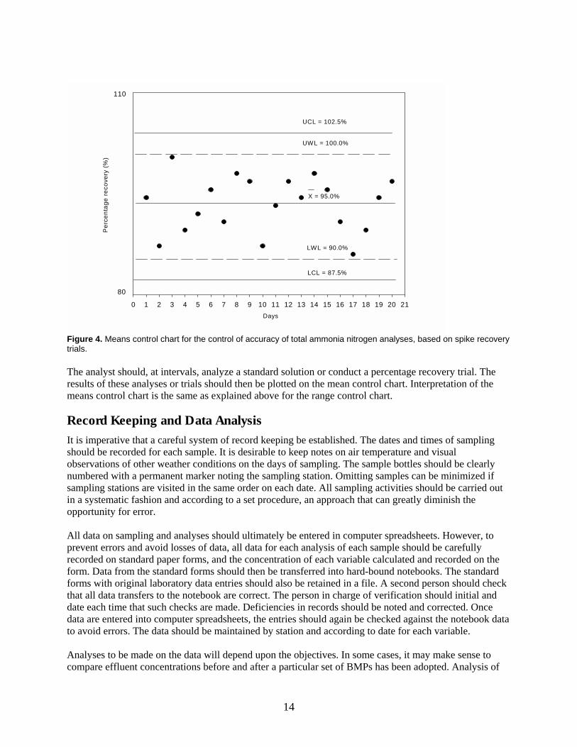
Figure 3. Means control chart for the control of accuracy of total phosphorus analyses (based on analyses of a standard solution). Alternatively, percentage recovery values can be used to make a means control chart. Suppose that percentage recovery values for total ammonia nitrogen averaged 95.0% with a standard deviation of ± 2.5. The limits would be as follows:

Upper control limit 102.5% Upper warning limit 100.0% Mean 95.0% Lower warning limit 90.0% Lower control limit 87.5%

These parameters are plotted as illustrated in Figure 4.

0 1 2 3 4 5 6 7 8 9 10 11 12 13 14 15 16 17 18 19 20 21

UCL = 0.32 mg/l

UWL = 0.30 mg/l

X = 0.26 mg/l

LWL = 0.22 mg/l

LCL = 0.20 mg/l

Mea

sure

d co

ncen

tratio

n (m

g/l)

0.35

0.15

Days

14

Figure 4. Means control chart for the control of accuracy of total ammonia nitrogen analyses, based on spike recovery trials. The analyst should, at intervals, analyze a standard solution or conduct a percentage recovery trial. The results of these analyses or trials should then be plotted on the mean control chart. Interpretation of the means control chart is the same as explained above for the range control chart.

Record Keeping and Data Analysis

It is imperative that a careful system of record keeping be established. The dates and times of sampling should be recorded for each sample. It is desirable to keep notes on air temperature and visual observations of other weather conditions on the days of sampling. The sample bottles should be clearly numbered with a permanent marker noting the sampling station. Omitting samples can be minimized if sampling stations are visited in the same order on each date. All sampling activities should be carried out in a systematic fashion and according to a set procedure, an approach that can greatly diminish the opportunity for error. All data on sampling and analyses should ultimately be entered in computer spreadsheets. However, to prevent errors and avoid losses of data, all data for each analysis of each sample should be carefully recorded on standard paper forms, and the concentration of each variable calculated and recorded on the form. Data from the standard forms should then be transferred into hard-bound notebooks. The standard forms with original laboratory data entries should also be retained in a file. A second person should check that all data transfers to the notebook are correct. The person in charge of verification should initial and date each time that such checks are made. Deficiencies in records should be noted and corrected. Once data are entered into computer spreadsheets, the entries should again be checked against the notebook data to avoid errors. The data should be maintained by station and according to date for each variable. Analyses to be made on the data will depend upon the objectives. In some cases, it may make sense to compare effluent concentrations before and after a particular set of BMPs has been adopted. Analysis of

0 1 2 3 4 5 6 7 8 9 10 11 12 13 14 15 16 17 18 19 20 21

UCL = 102.5%

UWL = 100.0%

X = 95.0%

LWL = 90.0%

LCL = 87.5%

110

80

Per

cent

age

reco

very

(%)

Days

15

variance techniques can be used to compare means of water quality variables before and after adoption of BMPs. The differences in water quality from one station to the next can also be evaluated by analysis of variance. Existence of water quality gradients from outfalls to more distant sampling stations can reveal adverse effects of effluents. Evidence in water quality deterioration over time can be established by comparing water quality data from each station over a period of several years (or over annual cycles). However, short-term changes in water quality can result from normal seasonal or annual variation in rainfall, temperature, or other weather conditions.

Costs

The costs for conducting a water quality monitoring program will vary with the size of the program, amount of existing equipment, and the country in which the program is to be conducted. The initial costs of the field and laboratory equipment (excluding boat and vehicle) would be around US$135,000 to US$150,000 . Reagents and other laboratory supplies would cost about US$20,000 per year. In order to design and operate the program in a reliable manner, a water quality consultant will be required. Including the cost of personal and operating expenses, we estimate that a medium-sized monitoring program (20 to 40 sampling stations) with biweekly sampling frequency could be done in most tropical nations for about US$300,000 during the first year and around US$150,000 per year for subsequent years. A budget breakdown is provided in Table 5. Table 5. Example of a budget for a water quality monitoring program with 20 to 40 sampling stations in a tropical nation

Item Year 1 (US$) Other years (US$) Vehicle 30,000 Gasoline and vehicle maintenance 5,000 5,000 Boat and motor 10,000 Operating costs for boat 2,000 2,000 Field equipment 10,000 5,000 Laboratory instruments, including AC, computer, generators etc.

85,000 10,000

Reagents and other lab supplies 20,000 15,000 Lab maintenance 5,000 6,000 Analyst 25,000 25,000 Lab assistants (2) 30,000 30,000 Secretary 10,000 10,000 Field assistant 12,000 12,000 Part-time help (laboratory and field) 10,000 10,000 Water quality consultant (travel and fee) 30,000 20,000 Telephone, office supplies, etc. 3,000 2,000 Utilities 5,000 5,000 Miscellaneous 2,000 2,000 Total 294,000 159,000 This budget assumes that a vehicle and boat would have to be purchased, all personnel would have to be salaried by project funds, all field and laboratory equipment would be purchased by the project, but it does not include the cost of laboratory space.

16

Performance Indicators For Monitoring Programs

Performance of a water quality monitoring program may be evaluated using the following parameters: • Review of laboratory quality control charts provides evidence on whether laboratory operations are

being performed with acceptable precision and accuracy. • The laboratory data forms and record books can be checked to determine whether entries are being

made according to the prescribed methods and checked. • Record books reveal whether samples are being taken according to the prescribed time schedule.

These books also provide evidence about whether all stations are being sampled and all variables measured.

• The water quality consultant should present an annual report providing his assessment of progress. An evaluation of laboratory compliance with performance indicators should be made in this report.

Effects of Effluents

The concentrations of water quality variables provide useful information on the relative pollution potential of effluents, but the pollution load cannot be estimated from concentration alone. The load of a pollutant in effluents can be determined only when both effluent volume and concentration of pollutant are known. For example, two effluents might each have a BOD of 15 mg/l, but volume might be 1,000 m3/day for one effluent and 100,000 m3/day for the other. The BOD load would be 15 kg/day for the smaller effluent and 1,500 kg/day for the larger effluent. Obviously, the pollution potential of the larger effluent is much greater than that of the smaller one. Shrimp farm discharge structures are not gauged for measuring flow rates or volumes. The best that can be done is to make indirect estimates of effluent volumes, but such estimates can often be made with a fair degree of accuracy. To illustrate, suppose that a shrimp farm has 1,000 ha of pond surface area and ponds are 1.2 m deep. The ponds are operated for 2.2 crops per year, and water exchange averages 5% per day. The production is staged so that harvest and restocking is done on as continuous a basis as possible, and about 50 ha of ponds are out of production (empty) at any given time. Calculation of the average daily effluent volume is made below.

Total pond volume, 1,000 ha x 10,000 m2/ha x 1.2 m = 12,000,00 m3

Water discharged for harvesting ponds, 12,000,000 m3 x 2.2 harvests/year = 26,400,000 m3/ year

Water discharged for water exchange, 950 ha x 10,000 m2/ha x 1.2m x 0.05 x 365 days/ year = 208,050,000 m3/year

Average daily effluent 234,450,000 ÷ 365 = 642,329 m3/day

Suppose that in the above example, it was found that the average BOD of the farm effluent was 9 mg/l. The daily BOD load would then be 5,781 kg/day. Of course, the water entering the farm would have a BOD as well, so all of the BOD in the effluent may not have originated from the shrimp production. The influence of pollution on a water body depends upon the input of pollutants and the capacity of the body of water to dilute and assimilate pollutants. Thus, larger and thoroughly mixed bodies of water that are well aerated by wind action have a greater capacity to dilute and assimilate pollution without negative

17

impacts on water quality and aquatic life than do smaller and less-mixed water bodies. Where there is rapid exchange of water between estuaries and the open sea through tidal action and currents, the potential for water pollution is greatly diminished. Thus, even when we know the pollution load from shrimp farming in coastal water, it is usually impossible to estimate the effects of this pollution load on coastal water quality, because the assimilative capacity of the coastal water is seldom known. Furthermore, even if this assimilative capacity is known, we would need to know the quantities of all natural inputs and all other inputs of pollutants from human activities to determine whether the effluent from shrimp farming would cause (or significantly contribute to) water quality impairment.

Because it is usually impossible to accurately predict the influence of effluents on water quality in aquatic ecosystems from concentrations and pollutant load data, monitoring programs are often conducted to determine whether water quality is deteriorating as the result of effluents. Two major considerations are whether pollution is negatively influencing water quality throughout the ecosystem, and whether there are localized effects of effluents in the areas of outfalls. For this reason, even where pollution loads are not great, measures should be taken to minimize adverse effects in the mixing zone (where effluents mix with natural waters). For example, a small but highly concentrated effluent might not cause overall degradation of water quality in an estuary, but it would likely cause water quality impairment in the mixing zone. For this reason, limits are often placed on maximum concentrations of pollutants in effluents, even when total pollution loads may be much less than the assimilative capacity of a water body. Concentration limits for pollutants are often administered using discharge permits in countries that have systems for regulating effluents. These limits must be established by considering the composition and discharge pattern of the effluents, other uses of the receiving water (especially the most beneficial use), the capacity of the receiving water to assimilate pollutants, the ability to treat effluents, and a variety of other factors. The permissible concentration in effluents depends both on effluent volume (pollutant loads) and receiving water characteristics, and acceptable concentrations in effluents are greater than acceptable concentrations within the receiving water body as a whole. Indeed, such concentrations may be somewhat greater in the mixing zone than in the water body as a whole. However, effluent limits should prevent toxicity and adverse environmental impacts within the mixing zone. Thus, we cannot make general suggestions on concentration limits for shrimp pond effluents. However, many environmental agencies have published suggested concentrations for water quality variables in aquatic ecosystems, i.e., those concentrations that should be maintained in bodies of water receiving effluents, in order to protect the existing aquatic ecosystems against adverse impacts. A set of water quality guidelines for protecting aquatic ecosystems (a modification of guidelines provided by the Australian and New Zealand Environmental and Conservation Council (1992)) is given in Table 1. It must be emphasized that these guidelines apply to the water bodies receiving effluents, and not to the effluents themselves. Estuarine Monitoring: An Example from Honduras

The shrimp culture industry in Honduras developed primarily on large, barren salt flats adjacent to dense mangrove forests that fringe the estuaries of the Gulf of Fonseca on the Pacific coast of Central America. These salt flats attracted developers because shrimp farms could be constructed without first having to clear land, and the high tidal amplitude in adjacent estuaries provided an easily accessed water source. Shrimp ponds there are managed semi-intensively, and Penaeus vannamei is the principal species cultured, although a few farms stock IHHNV-resistant P. stylirostris, especially during the dry season. Pond management practices in Honduras have been described by Teichert-Coddington (1995). Intake water for shrimp farms in Honduras comes from embayments of the Gulf of Fonseca, or riverine estuaries, which are influenced directly by seasonal variation in river discharge. Most shrimp farms in

18

Honduras have developed on salt flats along riverine estuaries of the Choluteca or Negro rivers. Southern Honduras experiences a seasonal climate with distinct rainy and dry seasons. Consequently, river discharge varies tremendously with season. Mean annual flow of the Choluteca River is about 45 m3/s, while peak flow can exceed 1,500 m3/s, and minimal flow might be less than 2 m3/s during prolonged dry weather. Flow data is not available for the Negro River; observations indicate that river discharge is negligible at the height of the dry season. Rainfall runoff from the coastal plain watershed also flows into estuaries and embayments via seasonal creeks. Farms usually discharge pond effluents into the same estuaries from which they and neighboring farms get their intake water.

Project Design and Implementation

Honduran government officials and shrimp farmers, aware of the environmental problems associated with shrimp culture in Asia and other parts of Latin America, were growing increasingly concerned in the early 1990s about the potential for environmental problems in Honduran shrimp culture. In response to this concern, a research project, developed as part of the Auburn University–Honduras Pond Dynamics/Aquaculture Collaborative Research Support Program (Honduras PD/A CRSP), was initiated in 1993 in southern Honduras to collect the water quality and hydrographic data necessary to estimate estuarine assimilative capacities, and to investigate production technologies for minimizing environmental impact. The Honduras PD/A CRSP had been active in inland aquacultural research and development since 1983. This project began as a broad collaborative effort of universities, the private sector, and the public sector (Table 6). Table 6. Participants in Honduras PD/A CRSP estuarine water quality monitoring and shrimp production research program.

Institution • Ministry of Agriculture and Livestock

General Directorate of Fisheries and Aquaculture Republic of Honduras

• Honduran National Association of Aquaculturists Choluteca, Honduras

• Panamerican Agriculture School Zamorano, Honduras

• Federation of Producers and Exporters of Honduras Choluteca, Honduras

• International Center for Aquaculture and Aquatic Environments Department of Fisheries and Allied Aquacultures Auburn University, Alabama

The Ministry of Agriculture and Livestock (MAL), through its General Directorate of Fisheries and Aquaculture (DIGEPESCA), is the Honduran government agency responsible for policy formulation and regulation in the fisheries/aquaculture sector; it dedicates significant effort to national aquacultural development. The Honduran National Association of Aquaculturists (ANDAH) represents 38 affiliated shrimp farms that together hold concessions for just over 19,600 ha of salt flats along the southern coast of Honduras, and manage a total pond area in production of 11,345 ha (ANDAH 1999, unpublished data). Individual concessions range from 20–5,200 ha. An additional 185 artisanal and small-scale producers, not affiliated currently with ANDAH, have operations ranging from 2–850 ha, with a total pond area in production of approximately 3,700 ha. More than 80% of these shrimp farms have less than 50 ha of pond area (ANDAH 1999, unpublished data).

19

The Panamerican Agricultural School (EAP) has a renowned educational program that integrates teaching of agricultural principles with field application; it graduates students who are capable farm and business managers. Project participation by EAP largely was limited to senior-year students conducting their senior thesis research (students were provided a stipend from project funds). The Federation of Producers and Exporters of Honduras (FPX) provides technical assistance to small- and medium-scale shrimp farmers and acts as a liaison between their client producers and ANDAH. Project participation by FPX continued through June 1994, when its aquacultural technical assistance project ended. A technical cooperation agreement that governed this project was drafted and signed by participants in September 1992. The agreement was later ratified by the president of Honduras, Dr. Carlos Roberto Reina, which increased its stature and legality. The goal of the agreement was to provide a scientific basis for estuarine management and sustainable development of shrimp culture in Honduras. Stated objectives of the technical cooperation agreement were to:

• Establish baseline data for selected chemical, physical, and biological variables in estuaries supplying water to shrimp farms, and in influent, effluent, and pond water;

• Optimize pond management practices for efficient fertilization, feeding, and water usage; • Develop extension materials and activities; and • Train technicians in water quality analysis and interpretation of results.

In the discussion of this case study, we report only on estuarine water quality monitoring activities. Responsibilities of project participants were described clearly in the technical cooperation agreement (Table 7). All participants were to acknowledge the collaboration and support of other participants in any publication that resulted from work conducted under the agreement. Administratively, the International Center for Aquaculture and Aquatic Environments (ICAAE) of Auburn University was the lead institution on all work done under the agreement. Project funding was provided by the US Agency for International Development (USAID), Auburn University, MAL-DIGEPESCA, and Honduran shrimp farmers (through ANDAH). The agreement could be modified by mutual consent of all parties, and was renewed annually by mutual accord. The Center for Research in Water Resources (CRWR), University of Texas at Austin, joined the project in September 1993 and provided expertise in estuarine dynamics. The CRWR was responsible for developing the estuarine carrying capacity models from data collected by other participants (Ward et al. 1999). A water chemistry laboratory was established in the heart of the shrimp-producing region at La Lujosa, Choluteca. Space for the laboratory (plus an electricity source and security) were provided by the Ministry of Agriculture and Livestock, at its La Lujosa Experiment Station, about 15 km west of Choluteca. Renovation of the provided space into a water quality laboratory was funded by ANDAH. Two air conditioners and a refrigerator were provided by FPX. Laboratory equipment, supplies, and reagents were purchased with Honduras PD/A CRSP funds. While the Honduras PD/A CRSP was operational, annual operating expenses were borne primarily by this project, with periodic contributions from USAID/Honduras and ANDAH. Beginning in 1997, ANDAH contributed US$10,000 annually towards laboratory operating expenses. In late 1998, USAID budget cuts forced termination of the Auburn University–Honduras PD/A CRSP shrimp culture activities. In response, ANDAH took full ownership of the laboratory and monitoring program, including all equipment, supplies, and the vehicle. A new bilateral agreement to continue the monitoring program was implemented between ANDAH and MAL in early 1999. Objectives of this new agreement focused on estuarine water quality monitoring.

20

Table 7. Specific responsibilities of signatories of the Honduras PD/A CRSP technical cooperation agreement in estuarine water quality and shrimp culture.

Institution Specific Responsibilities Ministry of Agriculture and Livestock (MAL), General Directorate of Fisheries and Aquaculture

• MAL will provide space at the La Lujosa Agricultural Experiment Station, Choluteca, to install a water quality laboratory and an office; and provide electricity, water and security for both.

• MAL will provide technical and maintenance personnel for the lab.

Honduran National Association of Aquaculturists • Members will provide a minimum of 12 ponds for pond trials.

• Members will provide all inputs required for each sampling effort and agree to carry all experiments to completion.

• Members will implement pond trials faithfully unless changes are agreed upon with ICAAE researchers.

• Farm technicians will collect water samples and transport them to the lab.

• Members will provide annual financial support for lab operation.

Panamerican Agriculture School (EAP) • EAP will organize and direct students interested in doing theses in shrimp culture and water quality.

• EAP will cooperate in the procurement and administration of local funds and other grants that may be secured to support the collaborative research detailed in the agreement.

Federation of Producers and Exporters of Honduras (FPX)

• FPX extensionists will assist in data collection from client farms, and with transferring research results to client farms.

• FPX will assist in the procurement of local currency and other donated funds to support the collaborative research detailed in the agreement.

International Center for Aquaculture and Aquatic Environments (ICAAE)

• ICAAE will implement in Honduras the activities specified under the terms of the existing Technical Cooperation Agreement between the Ministry of Agriculture and Livestock and Auburn University and provide funds to support those activities.

• ICAAE will designate a qualified ICAAE researcher to conduct activities detailed in the agreement.

• ICAAE will manage the water quality laboratory. • ICAAE will employ a Honduran chemist for the

laboratory. Two analysts and a technician constituted the laboratory staff. Occasional labor was contracted as needed to assist with glassware washing, lab maintenance, and janitorial services. Analysts processed 20–40 samples weekly, which included estuarine samples plus samples from pond production research projects. Analysts also entered data into a computer data base weekly. During the Honduras PD/A CRSP project, an in-country Auburn University researcher analyzed and reported the data on an annual basis. For the continued monitoring program, ANDAH must rely on a water quality consultant to oversee program implementation, data analysis, and reporting.

21

Sampling and Analyses

In Honduras, shrimp culture development is concentrated primarily along riverine estuaries (the Purgatorio, La Jagua, El Pedregal, San Bernardo, and La Berberia estuarine systems) in the eastern Gulf of Fonseca. Sampling sites for the estuarine monitoring program were not determined systematically, as recommended by Morris (1985), but rather by which farmers were willing to participate. Fortunately, most of the shrimp farms developed in close proximity to one another along these few riverine estuaries. The nature and budget of the Honduras PD/A CRSP project precluded the design and implementation of a more traditional estuarine sampling program, so one goal was reaching participation by as many farmers as possible within a given estuary. Water quality was being monitored every one to two weeks at 20 sites on 12 estuaries of the Gulf of Fonseca by late 1998 (Table 8). Table 8. Estuaries and number of sampling sites in the Gulf of Fonseca, Honduras in the estuarine water quality monitoring program

Estuary Estuary Type and Number of Sampling Sites

El Pedregal Riverine; 2 sites

San Bernardo Riverine; 3 sites

La Jagua Riverine; 2 sites

La Berberia Riverine; 2 sites

El Garcero Riverine; 1 site

Purgatorio Riverine; 1 site

Los Perejiles Riverine; 2 sites

Los Barancones Embayment; 1 site

Butus Embayment; 1 site

Golfo de Espabeles Embayment; 2 sites

Jiote Grande Embayment; 1 site

La Cutú Embayment; 1 site

Since the project began, the number of sites sampled weekly has varied from 13 to 20, with the number of estuaries varying from 6 to 12; both showed growth over time. Program participation dropped off following Hurricane Mitch in October 1998, but by July 1999 the number of sample stations participating actively in the monitoring program had returned to prehurricane levels. Although samples currently are collected from 20 sites along 12 estuaries, weekly participation in the program varies. For example, in any given month only about 80% of the sites sampled will be sampled each week during the month. Varying participation is attributed to many causes: farms closing for the dry season, farms going out of business, change of farm ownership, changes in managers or technical staff responsible for collection and delivery of water samples to the lab, logistical difficulties (e.g., no transport available), or distraction caused by crisis situations on farms. Maintenance of faithful program participation requires continuous attention. Producer participation is encouraged at informal meetings between researchers and producers, through frequent contact with ANDAH personnel, and through

22

presentation of current project results at ANDAH Board of Directors meetings and at ANDAH semiannual general assemblies. Estuarine water samples are collected from pump discharge on individual farms within one hour before and after high tide. It is assumed that the water samples collected represent a mixed water column sample of the estuary at the pump station because of the superficial vortex caused by the 60- to 90-cm diameter pump intakes. Samples are placed on ice and transported to the water quality laboratory, where analysis begins within 12 hours of collection. The Choluteca River is also sampled weekly at La Lujosa, which is located downstream from the city of Choluteca and upstream from tidal influence. Samples are analyzed for total settleable solids (APHA 1985), nitrate nitrogen by cadmium reduction to nitrite (Parsons et al. 1992), total ammonia nitrogen (Parsons et al. 1992), filterable reactive phosphorus (Grasshoff et al. 1983), chlorophyll a (Parsons et al. 1992), total alkalinity (by titration to pH 4.5 endpoint); salinity, reactive silicate (Strickland and Parsons 1977), and 2-d BOD (APHA 1985). Total nitrogen and total phosphorus are determined by nitrate and phosphate analysis, respectively, after simultaneous persulfate oxidation in a strong base (Grasshoff et al. 1983). Laboratory analyses were conducted principally in support of specific Honduras PD/A CRSP work plans and not as a public service for analysis on demand. Because analyses were conducted as part of a formal research project, shrimp farmers were not charged fees. Shrimp farmers participate actively in the monitoring program by collecting estuarine water samples weekly (whenever feasible) according to a standardized protocol and delivering the samples to the laboratory for analysis. Data collected in this project are considered to be in the public domain and may be published nationally or internationally. Farmers often request the results of the water quality analyses for the samples they send to the lab. Researchers initially felt that distribution of short-term sample data would put unnecessary and difficult demands on them to interpret week-to-week changes, in a study designed to identify long-term trends. However, because some producers themselves are interested in exploring data from their own farms, and to maintain farmers’ interest and participation, the water quality laboratory now prepares and distributes through ANDAH at the beginning of each month individual farm data for the previous month’s water quality analyses. These reports present only analytical results; data interpretation and reporting continue to be provided at the ANDAH general assemblies. Farmers can also request through ANDAH historical data for their farm or estuary, which is provided in electronic format. Annual project reports are now translated into Spanish for distribution to farmers through ANDAH. In addition, there is an ongoing effort to incorporate new farms into the program, to expand the data base to include new sites and new estuaries. Incorporating ANDAH in the process of data and report distribution increases the benefits the association can offer its membership (and thus attract members) as well as increase participation in the water quality monitoring program.

Results

No long-term trend in eutrophication has been observed from 1993 to October 1998, in either riverine or embayment estuaries, in shrimp-producing regions of southern Honduras. The area of shrimp ponds in production has increased from 9,250 ha in 1993 to 14,954 ha in 1999 (Figure 5), while total shrimp production has only increased from 1.53 x 107 kg whole shrimp in 1993 to an estimated 1.80 x 107 kg whole shrimp in 1999 (ANDAH 1999, unpublished data), primarily because of high mortality caused by Taura Syndrome Virus and White Spot Syndrome Virus.

23

Figure 5. Mean total nitrogen concentration in the riverine El Pedregal estuary and embayments of the Gulf of Fonseca from 1993 to 1998. Total nitrogen concentration trends in other monitored riverine estuaries were similar to El Pedregal estuaries. Solid horizontal line in each graph is the grand mean concentration during this period. In the Gulf of Fonseca region, water quality in riverine estuaries is influenced directly by seasonal variation in river discharge and watershed runoff, while embayments experience less seasonal variation in water quality. Rains in southern Honduras generally begin in May, remain strong through June, taper off during July and August, and resume during September and October. However, the effects of the 1997–1998 El Niño in Honduras were delayed and reduced rains. As a result, observed salinity, total nitrogen, and chlorophyll a concentrations were higher at sampling sites along riverine estuaries in comparison to 1996–1997 (Green et al. 1998). Nutrient concentrations in embayments were not affected noticeably by the El Niño. Nutrient concentrations in riverine estuaries follow a cyclical trend, with higher concentrations of total nitrogen and total phosphorus occurring during the dry season and lower concentrations occurring during the rainy season (Figures 5 and 6). Trends in nutrient concentrations in other riverine estuaries are similar to those shown in Figures 5 and 6. Total nitrogen and total phosphorus concentrations are higher in riverine estuaries than in embayments of the Gulf of Fonseca. Major regional climatic events such as El Niño, which provoked drought conditions in Honduras, exacerbate water quality problems in riverine estuaries of the Gulf of Fonseca. In normal years, seasonal rains increase river discharge and watershed runoff, which serve to dilute nutrient concentrations in riverine estuaries. While salinity in riverine estuaries may be reduced to zero or nearly so during the rainy season because of massive freshwater inflow, total nitrogen and total phosphorus concentrations decrease by only 10–30% because of nutrient load in inflow (Figures 5, 6, and 7). Changes in land-use patterns in the Gulf of Fonseca watershed also affect estuarine water quality, because of associated changes in runoff patterns and volumes. Catastrophic climatic events, such as Hurricane Mitch, provoked massive flooding in the estuarine areas of the Gulf of Fonseca. In addition, two important rivers, the Choluteca and Negro rivers, experienced changes in their courses after Mitch hit the area. Reduction of river flow in the pre-Mitch channels reportedly was moderate to severe. If these two rivers do not return completely to their pre-Mitch channels during the next rainy season, water quality in these riverine estuaries may deteriorate, and shrimp farms located along these riverine estuaries may be harmed.

0.00

0.50

1.00

1.50

2.00

2.50

3.00

3.50

Mar-89

Aug-89

Nov-89

Mar-90

Jul-90

Oct-90

Mar-91

Aug-91

Nov-91

Mar-92

Jul-92

Nov-92

Mar-93

Jul-93

Nov-93

Feb-94

Jun-94

Sep-94

T otal Nitro

El Pedregal Estuary

24

Figure 6. Mean total phosphorus concentration in the riverine El Pedregal estuary and embayments of the Gulf of Fonseca from 1993 to 1998. Total phosphorus concentration trends in other monitored riverine estuaries were similar to El Pedregal estuary’s. Solid horizontal line in each graph is the grand mean concentration during this period.

0.00

0.10

0.20

0.30

0.40

0.50

0.60

0.70

Mar-89

Aug-89

Nov-89

Mar-90

Jul-90

Oct-90

Mar-91

Aug-91

Nov-91

Mar-92

Jul-92

Nov-92

Mar-93

Jul-93

Nov-93

Feb-94

Jun-94

Sep-94

Total Phosphah

El Pedregal Estuary

0.00

0.05

0.10

0.15

0.20

0.25

Mar-89

Aug-89

Nov-89

Mar-90

Jul-90

Oct-90

Mar-91

Aug-91

Nov-91

Mar-92

Jul-92

Nov-92

Mar-93

Jul-93

Nov-93

Feb-94

Jun-94

Sep-94

Total Phosph

Embayments

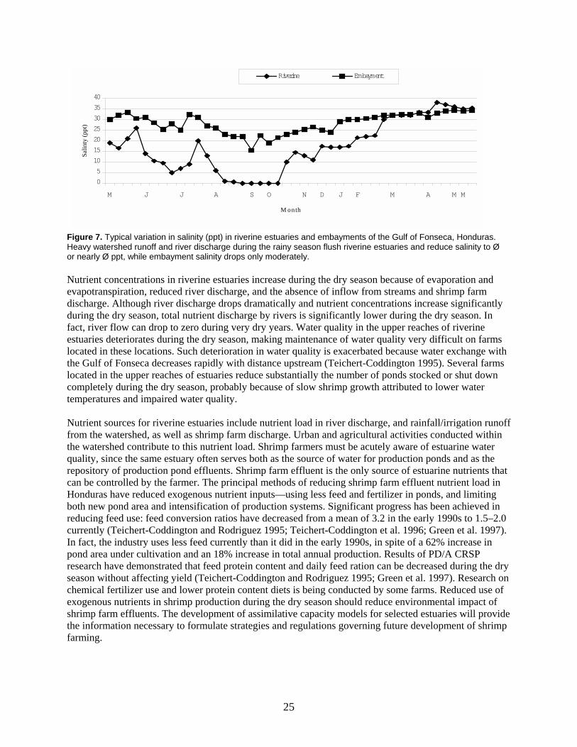
25

Figure 7. Typical variation in salinity (ppt) in riverine estuaries and embayments of the Gulf of Fonseca, Honduras. Heavy watershed runoff and river discharge during the rainy season flush riverine estuaries and reduce salinity to Ø or nearly Ø ppt, while embayment salinity drops only moderately. Nutrient concentrations in riverine estuaries increase during the dry season because of evaporation and evapotranspiration, reduced river discharge, and the absence of inflow from streams and shrimp farm discharge. Although river discharge drops dramatically and nutrient concentrations increase significantly during the dry season, total nutrient discharge by rivers is significantly lower during the dry season. In fact, river flow can drop to zero during very dry years. Water quality in the upper reaches of riverine estuaries deteriorates during the dry season, making maintenance of water quality very difficult on farms located in these locations. Such deterioration in water quality is exacerbated because water exchange with the Gulf of Fonseca decreases rapidly with distance upstream (Teichert-Coddington 1995). Several farms located in the upper reaches of estuaries reduce substantially the number of ponds stocked or shut down completely during the dry season, probably because of slow shrimp growth attributed to lower water temperatures and impaired water quality. Nutrient sources for riverine estuaries include nutrient load in river discharge, and rainfall/irrigation runoff from the watershed, as well as shrimp farm discharge. Urban and agricultural activities conducted within the watershed contribute to this nutrient load. Shrimp farmers must be acutely aware of estuarine water quality, since the same estuary often serves both as the source of water for production ponds and as the repository of production pond effluents. Shrimp farm effluent is the only source of estuarine nutrients that can be controlled by the farmer. The principal methods of reducing shrimp farm effluent nutrient load in Honduras have reduced exogenous nutrient inputs—using less feed and fertilizer in ponds, and limiting both new pond area and intensification of production systems. Significant progress has been achieved in reducing feed use: feed conversion ratios have decreased from a mean of 3.2 in the early 1990s to 1.5–2.0 currently (Teichert-Coddington and Rodriguez 1995; Teichert-Coddington et al. 1996; Green et al. 1997). In fact, the industry uses less feed currently than it did in the early 1990s, in spite of a 62% increase in pond area under cultivation and an 18% increase in total annual production. Results of PD/A CRSP research have demonstrated that feed protein content and daily feed ration can be decreased during the dry season without affecting yield (Teichert-Coddington and Rodriguez 1995; Green et al. 1997). Research on chemical fertilizer use and lower protein content diets is being conducted by some farms. Reduced use of exogenous nutrients in shrimp production during the dry season should reduce environmental impact of shrimp farm effluents. The development of assimilative capacity models for selected estuaries will provide the information necessary to formulate strategies and regulations governing future development of shrimp farming.

0

5

10

15

20

25

30

35

40

M J J A S O N D J F M A M M

M onth

Salin

ty (p

pt)

Riverine Embayment

26

Figure 8. Increase in shrimp pond area in production in southern Honduras since 1985. (Pond area for 2000 is estimated.) Water quality in the area’s embayments is less variable because embayments have better water exchange with the Gulf of Fonseca, which itself is low in nutrients (Figures 5 and 6). Data from all embayment estuaries are pooled because of the small number of sampling sites. In addition, the Gulf of Fonseca has a high tidal range (1.5–3.5 m), which promotes water exchange with the Pacific Ocean and results in nutrient dilution. River discharge and watershed runoff result in lower salinity in embayments, but not as low as those observed in riverine estuaries (Figure 7). Mean total nitrogen and total phosphorus concentrations increase from 11–25% during the rainy season because of nutrient load in river discharge and watershed runoff. Transitory spikes in nutrient concentration in embayments likely result from the concentration of farm effluents during low tides. In summary, estuarine water quality is generally good for shrimp culture during the rainy season, because river discharge and coastal plain runoff flush the estuaries. The potential for water quality problems is highest during the dry season, particularly upstream from the gulf where nutrients concentrate from lack of exchange with the gulf. A prolonged dry season, or inordinately high nutrient discharge, could eutrophy estuarine water, making it unsuitable for shrimp production. Farm development on salt flats far upstream should be discouraged because of the potential for poor water quality at such locations. Factors for Succes

Some of the factors responsible for the success of this project include a mature shrimp culture industry, a strong producers’ association, strong government interest, and good communication among all participants. The shrimp culture industry has reached maturity (Lara 1997); the land area under cultivation has stabilized, and there are few additional salt flats appropriate for expansion (Figure 8). The industry’s success provides significant incentive to work towards ensuring longevity. ANDAH, a strong, proactive industry association, represents more than half of the shrimp farmers active in Honduras and has an on-going effort to recruit as many producers as possible, including small-scale artisanal producers. The industry association has focused on the goal of sustainable production since 1992 and in 1995 formally amended its statutes to incorporate the concept of sustainability as a key element in its development strategy (Lara, 1997). The strength of ANDAH comes from its dedicated leadership and from the open communication and exchange of information among its members. The Government of Honduras, through strong leadership by

0

2,000

4,000

6,000

8,000

10,000

12,000

14,000

16,000

1985 1986 1987 1988 1989 1990 1991 1992 1993 1994 1995 1996 1997 1998 1999 2000

Year

Tota

l Pon

d A

rea

(ha)

27

the Ministry of Agriculture and Livestock, plays a vital role in setting the policy and regulatory framework that permits successful development of the shrimp industry within limits that protect the country’s interests above those of individual producers. Shrimp culture since 1984 has become important to the Honduran economy; it is currently the third largest earner of foreign exchange, generating an estimated US $88 million in 1997 (Lara, 1997). The Secretaría de Agricultura y Ganadería and ANDAH collaborate on a number of initiatives that affect the shrimp industry. There is frank, open dialog—although not always agreement—between the Government of Honduras and ANDAH, which is important to maintaining relations between the two parties. Finally, there is open and timely communication among researchers, producers, and government officials regarding project progress and results. We believe that the design and implementation of this project could serve as a model for other shrimp-producing countries, from those with a long history of shrimp production to countries where it is beginning to develop. This model is not limited to shrimp culture but could be applied also to other aquacultural activities.

28

Bibliography

American Public Health Association (APHA). 1985. Standard Methods for the Examination of Water and Wastewater. American Public Health Association (APHA), Washington, D.C., USA.

Australian and New Zealand Environment and Conservation Council (ANZECC). 1992. Australian Water

Quality Guidelines for Fresh and Marine Waters. ANZECC, Canberra, ACT, Australia. Boyd, C.E. and L. Massaut. 1999. Risks associated with the use of chemicals in pond aquaculture.

Aquacultural Engineering 20:113-132. Boyd, C.E. and C.S. Tucker. 1992. Water Quality and Pond Soil Analysis for Aquaculture. Alabama

Experiment Station, Auburn University, Auburn, AL, USA. Clesceri, L.S., A.E. Greenberg and A.D. Eaton. 1998. Standard Methods for the Examination of Water

and Wastewater. American Public Health Association (APHA), Washington, D.C., USA. Grasshoff, K., M. Ehrhardt and K. Kremling. 1983. Methods of Seawater Analysis. Verlag Chemie,

Weinheim, Germany. Green, B.W., D.T. Teichert-Coddington, C.E. Boyd, D. Martinez and E. Ramirez. 1998. Estuarine water

quality monitoring and estuarine carrying capacity. In D. Burke, J. Baker, B. Goetze, D. Clair, and H. Egna (eds) Fifteenth Annual Administrative Report, 1997, Pond Dynamics/Aquaculture CRSP, Oregon State University, Corvallis, OR, USA, pp. 87-98.

Green, B.W., D.T. Teichert-Coddington, C.E. Boyd, J.L. Harvin, H. Corrales, R. Zelaya, D. Martinez and

E. Ramirez. 1997. Effect of diet protein on food conversion and nitrogen discharge during semi-intensive production of Penaeus vannamei during the dry season. In H. Egna, B. Goetze, D. Burke, M. McNamara, and D. Clair (eds) Fourteenth Annual Administrative Report, 1996, Pond Dynamics/Aquaculture CRSP, Oregon State University, Corvallis, OR, USA, pp. 77-86.

Gross, A. and C.E. Boyd. 1998. Digestion procedure for the simultaneous determination of total nitrogen

and total phosphorus in pond water. Journal of the World Aquaculture Society 29:300-303. Gross, A., C.E. Boyd and J. Seo. 1999. Evaluation of the ultraviolet spectrophotometric method for the

measurement of total nitrogen in water. Journal of the World Aquaculture Society 30:388-393.

Lara, C.A. 1997. Sostenibilidad de la industria camaricultora de Honduras. Asociación Nacional de

Acuacultores de Honduras, Choluteca, Honduras. Morris, A.W. 1985. Estuarine chemistry and general survey strategy. In P.C. Head (ed) Practical

Estuarine Chemistry: A Handbook. Cambridge University Press, Cambridge, UK, pp. 1-60. Parsons, T.R., Y. Maita and C.M. Lalli. 1992. A Manual of Chemical and Biological Methods for

Seawater Analysis. Pergamon Press, New York, USA. Strickland, J.D.H. and T.R. Parsons. 1977. A Practical Handbook of Seawater Analysis (Bulletin 167).

Fisheries Research Board of Canada, Ottawa.

29

Teichert-Coddington, D.R. 1995. Estuarine water quality and sustainable shrimp culture in Honduras. In C.L. Browdy and J.S. Hopkins (eds) Swimming Through Troubled Waters, Proceedings of the special session on shrimp farming, Aquaculture ‘95. World Aquaculture Society, Baton Rouge, LA, USA, pp. 144-156.

Teichert-Coddington, D.R. and R. Rodriguez. 1995. Semi-intensive commercial grow-out of Penaeus

vannamei fed diets containing differing levels of crude protein during wet and dry seasons in Honduras. Journal of the World Aquaculture Society, 26:72-79.

Teichert-Coddington, D.R., W. Toyofuku, J. Harvin, and R. Rodriguez. 1996. Relationships among

stocking density, survival and yield in ponds affected by the Taura Syndrome during wet and dry seasons in Honduras. In H. Egna, B. Goetze, D. Burke, M. McNamara, and D. Clair (eds) Thirteenth Annual Administrative Report, 1995 Pond Dynamics/Aquaculture CRSP, Oregon State University, Corvallis, OR, USA, pp. 85-94.

United States Environmental Protection Agency. 1972. Handbook for Analytical Quality Control in Water

and Wastewater Laboratories. Analytical Quality Control Laboratory, Cincinnati, Ohio, USA.

Verdouw, H., C.J.A van Echteld and E.M.J. Dekkers. 1978. Ammonia determination based on indophenol

formation with sodium salicylate. Water Research 12:399-402. Ward, G.H., B.W. Green and D.R. Teichert-Coddington. 1999. Estimation of carrying capacity of shrimp

aquaculture in the eastern estuaries of the Gulf of Fonseca. In B.W. Green, H.C. Clifford, M. McNamara, and G. Montaño (eds) V Central American Symposium on Aquaculture: Aquaculture and Environment Together Towards the New Millennium, 18-20 August 1999, San Pedro Sula, Honduras. Asociación Nacional de Acuicultores de Honduras, Latin American Chapter of the World Aquaculture Society, and Pond Dynamics/Aquaculture Collaborative Research Support Program, Choluteca, Honduras, pp. 34-63.

The World Bank - Netherlands Partnership Program

The World Bank1818 H Street, NWWashington D.C. 20433-1234, USATelephone : 202-477-1234Facsimile : 202-477-6391Telex : MCI 64145 WORLDBANK MCI 248423 WORLDBANKWeb page : www.worldbank.orgE-mail : rzweig@worldbank.org

Network of Aquaculture Centres in Asia-Pacific (NACA)

Department of FisheriesKasetsart University CampusLadyao, Jatujak,Bangkok 10900, ThailandWeb page : www.enaca.orgE-mail : shrimp@enaca.org

World Wildlife Fund (WWF)

1250 24th Street, NWWashington D.C. 20037, USAWeb page : www.worldwildlife.orgE-mail : shrimp.aquaculture@wwfus.org

Food and Agriculture Organization of the United Nations (FAO)

Viale delle Terme di CarracallaRome 00100, ItalyWeb page : www.fao.orgE-mail : FI-Inquiries@fao.org

recycled paper