coarse matching and price discrimination - yale...

Coarse Matching and Price Discrimination

H. Hoppe, B. Moldovanu, and E. Ozdenoren

Slides by Adam Kapor, Sofia Moroni and Aiyong Zhu, April 1, 2011

H. Hoppe, B. Moldovanu, and E. Ozdenoren () Coarse Matching and Price DiscriminationSlides by Adam Kapor, Sofia Moroni and Aiyong Zhu, April 1, 2011 1

/ 32

introduction

Research Question

Two kinds of agents (“men”, “women”) look for a match.

An intermediary can extract transfers and match agents based on theirreported types.

▶ randomly?▶ coarsely?▶ assortatively?

RQ: How good is coarse matching with two categories for each kind of agent,relative to efficient matching or random matching?

▶ total surplus▶ agents’ utility▶ matchmaker’s revenue

Look for lower bounds.


/ 32

introduction

Motivation

Extend McAfee (2002)▶ Obtain lower bounds on surplus in more environments.▶ Private types mean that the matching must be incentive compatible.

Authors’ motivation: If coarse matching is “pretty good” in the worst case,then (unmodeled) costs of using a finer scheme may offset the benefits.

Why do firms offer a “small” menu of qualities?▶ One reason: a price-discriminating monopolist can get “close” to maximum

revenue with two quality levels.


/ 32

Model

Model

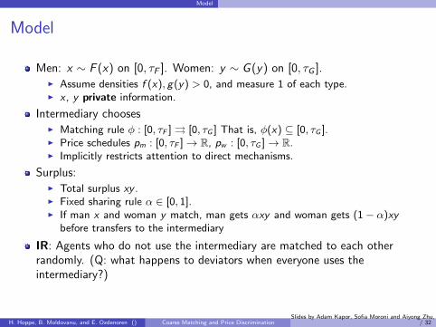
Men: x ∼ F (x) on [0, �F ]. Women: y ∼ G (y) on [0, �G ].▶ Assume densities f (x), g(y) > 0, and measure 1 of each type.▶ x , y private information.

Intermediary chooses▶ Matching rule � : [0, �F ] ⇉ [0, �G ] That is, �(x) ⊆ [0, �G ].▶ Price schedules pm : [0, �F ]→ ℝ, pw : [0, �G ]→ ℝ.▶ Implicitly restricts attention to direct mechanisms.

Surplus:▶ Total surplus xy .▶ Fixed sharing rule � ∈ [0, 1].▶ If man x and woman y match, man gets �xy and woman gets (1− �)xy

before transfers to the intermediary

IR: Agents who do not use the intermediary are matched to each otherrandomly. (Q: what happens to deviators when everyone uses theintermediary?)


/ 32

Model

What do matchings look like?

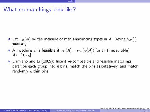
Let �M(A) be the measure of men announcing types in A. Define �W (.)similarly.

A matching � is feasible if �M(A) = �W (�(A)) for all (measurable)A ⊆ [0, �G ]

Damiano and Li (2005): Incentive-compatible and feasible matchingspartition each group into n bins, match the bins assortatively, and matchrandomly within bins.


/ 32

Assortative Matching

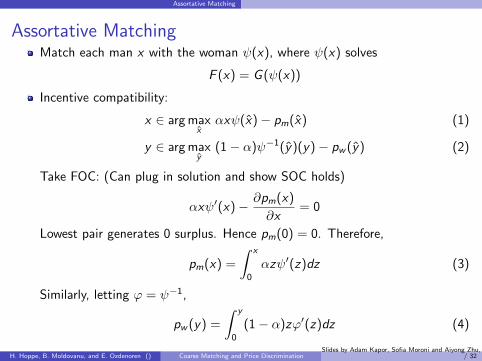
Assortative MatchingMatch each man x with the woman (x), where (x) solves

F (x) = G ( (x))

Incentive compatibility:

x ∈ arg maxx

�x (x)− pm(x) (1)

y ∈ arg maxy

(1− �) −1(y)(y)− pw (y) (2)

Take FOC: (Can plug in solution and show SOC holds)

�x ′(x)− ∂pm(x)

∂x= 0

Lowest pair generates 0 surplus. Hence pm(0) = 0. Therefore,

pm(x) =

∫ x

0

�z ′(z)dz (3)

Similarly, letting ' = −1,

pw (y) =

∫ y

0

(1− �)z'′(z)dz (4)


/ 32


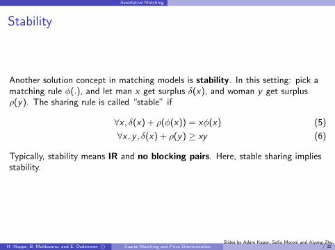
Stability

Another solution concept in matching models is stability. In this setting: pick amatching rule �(.), and let man x get surplus �(x), and woman y get surplus�(y). The sharing rule is called “stable” if

∀x , �(x) + �(�(x)) = x�(x) (5)

∀x , y , �(x) + �(y) ≥ xy (6)

Typically, stability means IR and no blocking pairs. Here, stable sharing impliesstability.


/ 32


Stability and efficiency

Claim: the stable matching must be assortative.

First, show a stable matching must be monotone increasing. Take x ′ > x ,y ′ > y , and for a contradiction, suppose a stable sharing rule assigns x ↔ y ′

and x ′ ↔ y .

�(x) + �(y ′) = xy ′

�(x ′) + �(y) = x ′y

=⇒ �(x) + �(y) + �(x ′) + �(y ′) = x ′y + xy ′

xy + x ′y ′ ≤ x ′y + xy ′

Hence (x ′ − x)(y ′ − y) ≤ 0

If x ∕↔ (x), then wlog say x ↔ y > (x). Then, since g(.) > 0, we haveG (y) = G ( (x)) + � for some � > 0. If the matching is monotone increasing,then �m([x , �F ]) ≥ �w (�([x , �F ])) + �.

To summarize, if a matching rule is stable, either it is infeasible or it is assortative.


/ 32


Stable shares

Differentiate �(x) + �( (x)) = x (x). Obtain

�′(x) + �′( (x)) ′(x) = (x) + x ′(x)

Matching coefficients, �′(x) = (x), and �′(�(x)) = x .

We know that �(0) = �(0) = 0.

Hence, by the FTC the stable shares are

�(x) =

∫ x

0

(z)dz (7)

�(y) =

∫ y

0

'(z)dz (8)


/ 32


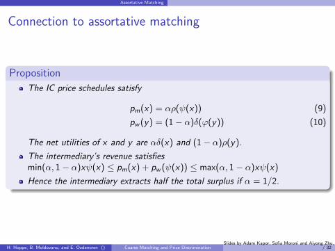
Connection to assortative matching

Proposition

The IC price schedules satisfy

pm(x) = ��( (x)) (9)

pw (y) = (1− �)�('(y)) (10)

The net utilities of x and y are ��(x) and (1− �)�(y).

The intermediary’s revenue satisfiesmin(�, 1− �)x (x) ≤ pm(x) + pw ( (x)) ≤ max(�, 1− �)x (x)

Hence the intermediary extracts half the total surplus if � = 1/2.


/ 32


Proof of prop 1-1

Total surplus from a pair is u(x , (x)) = x (x). Totally differentiate:

d

dxu(x , (x)) = (x) + x ′(x)

By the FTC, u(x , (x)) =∫ x

0 (z)dz +

∫ x

0z ′(z)dz . Hence

�u(x , (x)) = �

∫ x

0

(z)dz︸︷︷︸��(x)

+�

∫ x

0

z ′(z)dz︸︷︷︸pm(x)

Also, using a change of variables w = (z), we have1�pm(x) =

∫ x

0z ′(z)dz =

∫ (x)

0'(w)dw = �( (x)).


/ 32


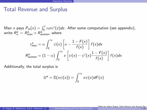
Total Revenue and Surplus

Man x pays Pm(x) =∫ x

0�z ′(z)dz . After some computation (see appendix),

write Ra� = Ra

men + Rawomen, where

r amen = �

∫ �F

0

(x)

[x − 1− F (x)

f (x)

]f (x)dx

Rawomen = (1− �)

∫ �F

0

x

[ (x)− ′(x)

1− F (x)

f (x)

]f (x)dx

Additionally, the total surplus is

Ua = E(x (x)) =

∫ �F

0

x (x)dF (x)


/ 32

Coarse Matching

Why Coarse Matching?

Perfect (Assortative) matching incurs various transaction costs:▶ Intermediary: communication (decoding) cost▶ Agents: evaluation (coding) cost

Agents only need to reveal partial information.

In terms of total surplus, the intermediary’s revenue and agents’s welfare:▶ It is significantly higher than completely random matching.▶ It may achieve a large proportion of assortative matching.


/ 32

Coarse Matching

Coarse Matching Model

�

∫ y

0

xy

G (y)dG (y) = �

∫ �G

y

xy

1− G (y)dG (y)− pc

m (11)

(1− �)

∫ x

0

xy

F (x)dF (x) = (1− �)

∫ �F

x

xy

1− F (x)dG (y)− pc

w (12)

y = (x) (13)

two classes: willing to pay and not willing to pay

x(y) the lowest type of men (women) who is willing to pay pcm(pc

w ).

such pricing scheme is incentive compatible.


/ 32

Coarse Matching

Coarse Matching Model

cutoff point: x = EX , and y = (Ex)

EXL = EX −∫ EX

0F (x)dx

F (EX ),EYL = (EX )−

∫ (EX )

0G (x)dx

G ( (EX ))

total surplus: UEX

=

∫ EX

0

∫ (EX )

0

xy

F (EX )dG (y)dF (x) +

∫ �F

EX

∫ �G

(EX )

xy

1− F (EX )dG (y)dF (x)

= EXEY +F (EX )

1− F (EX )(EX − EXL)(EY − EYL)

intermediary’s revenue (fix � = 1/2):

REX = [1− F (EX )]pcw + [1− G ( (EX ))]pc

m

=1

2[EX (EY − EYL) + (EX )(EX − EXL)]


/ 32

Coarse Matching

Total Surplus

Note definition 2:Ua = (1 + CCV 2(x , (x)))U r

If the distributions F and G both satisfy:1 F and G are both log-concave (F ,G DRFR)1

2 (1-F) and (1-G) are both log-concave (F ,G IFR)2

UEX ≥ Ua + U r

2⇒ UEX ≥ 3

4Ua,UEX ≥ U r

If F and G are both concave and is convex, then:

UEX ≥ 5

4U r

1decreasing reversed failure rate f (t)F (t)

2increasing failure (hazard) rate f (t)1−F (t)


/ 32

Coarse Matching

Total Surplus

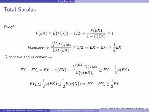
Proof:

F (EX ) ≥ E (F (X )) = 1/2⇒ F (EX )

1− F (EX )≥ 1

Fconcave ⇒∫ EX

0F (x)dx

EXF (EX )≥ 1/2⇒ EX − EXL ≥

1

2EX

G concave and convex ⇒

EY − EYL = EY − (EX ) +

∫ (EX )

0G (x)dx

G ( (EX ))≥ EY − 1

2 (EX )

EYL ≤1

2 (EX ) ≤ 1

2E ( (X ))⇒ EY − EYL ≥

1

2EY


/ 32

Coarse Matching

Intermediary’s Revenue

If the distributions F and G both satisfy:1 F and G are both concave2 (1-F) and (1-G) are both log-concave (F ,G IFR)

REX ≥ 1

2Ra

Intuition: As the distribution of types on the other market side becomes moreconcave, the mass of potential partners with very low type gets larger,leading to a higher revenue since agents in high class are willing to pay more.

If EX ≥ EY and is convex, then REXm ≥ REX

w

Intuition: If F and G have the same mean, but G has a higher variance, thechances for men to match with a lower type of women are higher thanwomen, thus men in higher class are willing to pay more.


/ 32

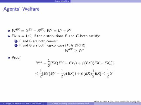
Coarse Matching

Agents’ Welfare

W EX = UEX − REX , W a = Ua − Ra

Fix � = 1/2, if the distributions F and G both satisfy:1 F and G are both convex2 F and G are both log-concave (F ,G DRFR)

W EX ≥W a

Proof

REX =1

2[EX (EY − EYL) + (EX )(EX − EXL)]

≤ 1

2[EX (EY − 1

2 (EX )) + (EX )

1

2EX ] ≤ 1

2U r


/ 32

Coarse Matching

Agents’ Welfare

W EX = UEX − REX

≥ 1

2(Ua + U r )− 1

2U r =

1

2Ua = W a

However,

W r = U r =1

1 + CCV 2(x , (x))

≥ 1

2Ua = W a


/ 32

Price Discrimination

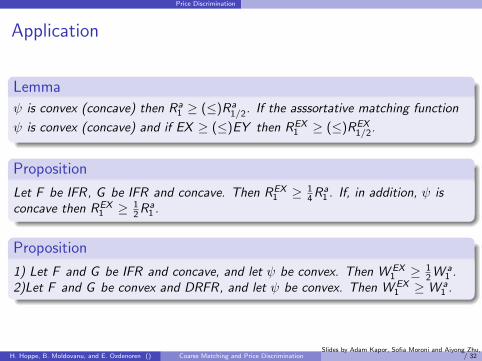
Application

Lemma

is convex (concave) then Ra1 ≥ (≤)Ra

1/2. If the asssortative matching function

is convex (concave) and if EX ≥ (≤)EY then REX1 ≥ (≤)REX

1/2.

Proposition

Let F be IFR, G be IFR and concave. Then REX1 ≥ 1

4 Ra1 . If, in addition, is

concave then REX1 ≥ 1

2 Ra1 .

Proposition

1) Let F and G be IFR and concave, and let be convex. Then W EX1 ≥ 1

2 W a1 .

2)Let F and G be convex and DRFR, and let be convex. Then W EX1 ≥W a

1 .


/ 32


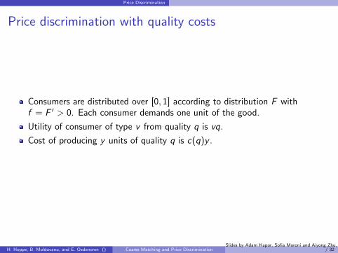
Price discrimination with quality costs

Consumers are distributed over [0, 1] according to distribution F withf = F ′ > 0. Each consumer demands one unit of the good.

Utility of consumer of type v from quality q is vq.

Cost of producing y units of quality q is c(q)y .


/ 32


Revenue maximizing profit function

By the standard mechanism design argument we know that monopolist’s revenue and profit aregiven by

Ra =

∫ 1

0q(v)

(v −

1− F (v)

f (v)

)f (v)dv

and

�a1 =

∫ 1

0

[q(v)

(v −

1− F (v)

f (v)

)− c(q(v))

]f (v)dv

Let r be such that(r − 1−F (r)

f (r)

)= 0. Solution is,

q(v) = 0 if v ≤ r

c ′(q(v)) = v −1− F (v)

f (v)if v ≥ r

Define G(y) = F (q−1(y)) we get a distribution of quality levels where q(v) = (v) valuation

(men), quality (women).


/ 32


Price discrimination example

In paper’s framework: total revenue of the assortative matching is given by(� = 1)

Ra1 =

∫ �F

0

(x)

(x − 1− F (x)

f (x)

)dF (x)

(from computing E(pm))

Coarse matching: provide two qualities QL =∫ EV

0q(z)dF (z)/F (EV ) and

QH =∫ 1

EVq(z)dF (z)/(1− F (EV )) and REV

1 = EV (EQ − QL)


/ 32


Example

c(q) = q2 and v ∼ U[0, 1]. In this case, q(v) = 0 if v ≤ 12 and r = 1/2 and

2q(v) = v − 1−v1 ⇐⇒ q(v) = 2v−1

2

G (y) = 1+2y2 for y ∈

[0, 1

2

]which is concave and IFR.

Computation yields QH = 12 , Ra

1 = 112 , REV

1 = 116 that is REV

1 = 34 Ra

1 . (noteProp 9 tells us REX

1 ≥ 12 Ra

1 )

Total profit is given by �a1 = 1

24 and �EV1 = 1

32 and �EV1 = 3

4�a.

W EV = 132 >

148 = W a (note Prop 10 tells us W EV ≥W a).


/ 32


Proof of Lemma 4

Lemma

is convex (concave) then Ra1 ≥ (≤)Ra

1/2. If the asssortative matching function

is convex (concave) and if EX ≥ (≤)EY then REX1 ≥ (≤)REX

1/2.

Proof

dRa

d�=

∫ 1

0(x ′(x)− (x))(1− F (x))dx > 0

if convex. That is Ra� increasing in �.

Now, note EX ≥ EY = E (X ) ≥ (EX ) if convex (concave) and (EY − EYL) ≥ (EX − EXL)by Lemma 3.

REX1 = EX (EY − EYL) ≥

1

2[EX (EY − EYL) + (EX )(EX − EXL)] = REX

1/2


/ 32


Proof of Proposition 9

Proposition

Let F be IFR, G be IFR and concave. Then REX1 ≥ 1

4Ra

1 . If, in addition, is concave then

REX1 ≥ 1

2Ra

1 .

Proof.

By Lemma 3 EY − EYL ≥ 12EY if G is concave. This yields

REX1 = EX (EY − EYL) ≥

1

2EXEY =

1

2Ur =

1

2

(EX (X )

1 + CCV 2(X , (X ))

)

=1

2

(Ua

1 + CCV 2(X , (X ))

)≥

1

2

(Ra

1

1 + CCV 2(X , (X ))

)CCV 2(X , (X )) ≤ 1 if F and G are both IFR. Ua ≥ Ra

1 in general and if concave Ra1 < Ra

1/2,

and since Ua = 2Ra1/2

, Ua > 2Ra1 .


/ 32


Proof of Proposition 10

Proposition

1) Let F and G be IFR and concave, and let be convex. Then W EX1 ≥ 1

2W a

1 . 2)Let F and G

be convex and DRFR, and let be convex. Then W EX1 ≥W a

1 .

Proof 1)

UEX = EXEY +F (EX )

1− F (EX )(EX − EXL)(EY − EYL)

F (X ) ≥ 1/2 by L2

≥ EXEY + (EX − EXL)(EY − EYL)

algebra= REX

1 + EY (EX − EXL) + EYLEXL

EX − EXL ≥ 1/2EX by L3

≥ REX1 +

1

2EXEY + EYLEXL

algebra=

3

2REX

1 +1

2EXEYL + EYLEXL =⇒ UEX >

3

2REX

1


/ 32


Proof of Proposition 10 continued

Now,

W EX1 = UEX − REX

1

23UEX > REX

1

≥1

3UEX

McAfee≥

1

3

1

2(Ua + Ur )

Ur ≥ 1/2Ua if F and G IFR

≥1

6(Ua +

1

2Ua) =

1

4Ua

Ua/2 > Ra1 if cvx

≥1

2W a

1

2)

REX1 = EX (EY − EYL)

L3, F and G cvx≤

1

2EXEY =

1

2Ur

This implies that

W EX1 = UEX − REX

1 ≥1

2(Ua + Ur )−

1

2Ur =

1

2Ua

Ua/2 > Ra1 if cvx

≥ W a1


/ 32

Conclusion

Conclusions

Simple matching schemes can work under incomplete information, and arenot too far from optimal, even in the worst case.

▶ But how easy is it to satisfy the statistical assumptions?▶ Horizontally differentiated goods?

... we focus on clearly suboptimal mechanisms, while identifyingsettings where such mechanisms are very effective (and thus maybecome optimal once transaction costs associated with morecomplex mechanisms are taken into account.

Foundations for costs of complexity?


/ 32

Assortative matching revenue: men’s shareMan x pays Pm(x) =

∫ x

0�z ′(z)dz . Integrating by parts,

pm(x) = (x)x −∫ x

0

(z)dz

Take the expectation over all men:

Ramen =

∫ �F

0

Pm(x)f (x)dx

= �

⎛⎝∫ �F

0

(x)xf (x)dx −∫ �F

0

∫ x

0

(z)dzf (x)dx︸︷︷︸⎞⎠

∫ �F

0

∫ �

z

f (x)dx (z)dz =∫ �F

0

(1− F (z)) (z)dz =

Ramen = �

∫ �F

0

(x)

[x − 1− F (x)

f (x)

]f (x)dx


/ 32

SOC for assortative matchingPlugging in the solution to the FOC, man x solves

arg maxx�

(x (x)−

∫ x

0

z ′(z)dz

)

=�(x − x) (x) + �

⎛⎜⎜⎜⎜⎝x (x)−∫ x

0

z ′(z)dz︸︷︷︸x (x)−

∫ x0 (z)dz

⎞⎟⎟⎟⎟⎠=�(x − x) (x) + �

∫ x

0

(z)dz

d

dx:�(x − x) ′(x)

d2

dx2: (x − x) ′′(x)︸︷︷︸

=0 at x=x

− ′(x) < 0

The above shows that at reporting x = x gives a local maximum. Since thesolution to the FOC is unique, we need to rule out only reporting 0 or reporting � .


/ 32

coarse matching and price discrimination - yale...

Documents