Coarse graining, dynamic renormalization and the

kinetic theory of shock clustering

Xingjie Li ∗, Matthew O. Williams †, Ioannis G. Kevrekidis ‡,

Govind Menon §

December 23, 2015

Keywords: Dynamic scaling, equation free method, Smoluchowski’s coagu-lation equation, sticky particles, Burgers turbulence, Uncertainty quantifi-cation.

Abstract

We demonstrate the utility of the equation-free methodology de-veloped by one of the authors (I.G.K) for the study of scalar conser-vation laws with disordered initial conditions. The numerical schemeis benchmarked on exact solutions in Burgers turbulence correspond-ing to Levy process initial data. For these initial data, the kineticsof shock clustering is described by Smoluchowski’s coagulation equa-tion with additive kernel. The equation-free methodology is used todevelop a particle scheme that computes self-similar solutions to thecoagulation equation, including those with fat tails.

∗Work completed at Division of Applied Mathematics, Brown University, 182 GeorgeSt., Providence, RI 02912, USA. Current address: Department of Mathematics and Statis-tics, University of North Carolina, Charlotte, NC 28223. Email: xli47@uncc.edu.

†Work completed at Program for Applied and Computational Mathematics and De-partment of Chemical and Biological Engineering, Princeton University, 6 Olden St.,Princeton, NJ 08544, USA. Current address: United Technologies Research Center, 411Silver Lane, East Hartford, CT 06118, USA. Email: william1@utrc.utc.com.

‡Program for Applied and Computational Mathematics and Department of Chemicaland Biological Engineering, Princeton University, 6 Olden St., Princeton, NJ 08544, USA.Email: yannis@princeton.edu.

§Division of Applied Mathematics, Brown University, 182 George St., Providence, RI02912, USA, Email: govind menon@brown.edu.

1

1 Introduction

Model problems in turbulence play an important role in guiding the anal-ysis of complex stochastic systems. Our purpose in this paper is to illus-trate the utility of a class of exact solutions in Burgers turbulence – thestudy of Burgers equation with random initial data – as a means to developand benchmark numerical methods to study the evolution of ensembles ofsolutions to complex systems. The exact solvability of finite-dimensionaltruncations of Burgers equation has been used to illustrate strategies formodel-reduction and coarse-graining (e.g. [12, 15]). The exact solutionsthat underlie this work are infinite-dimensional, as explained below, andrequire a different coarse-graining strategy. Our work combines two recentadvances– (a) the development of equation-free numerical schemes for mul-tiscale problems [1, 14]; and (b) the development of a kinetic theory for shock

clustering in scalar conservation laws with random initial data [16, 18, 19].The essence of the equation free method is to extract the evolution of

coarse macroscopic statistics for a system of microscopically evolving parti-cles by designing many brief parallel “bursts” of short-time evolution for themicroscopic system. Equation-free schemes are of most value when the mi-croscopic evolution is fast and complex (given for example, by a detailed, butexpensive, multiphysics code), but the evolution of macroscopic variables isslow and their evolution equations unknown. The fact that the closed evolu-tion equations for the macroscopic statistics are unknown, or not known inclosed form, is what makes these methods “equation-free”. Nevertheless, asin all numerical methods, it is important to validate these schemes on modelsystems that are reasonably complex, but for which closed form equationsfor the coarse-grained problem are available.

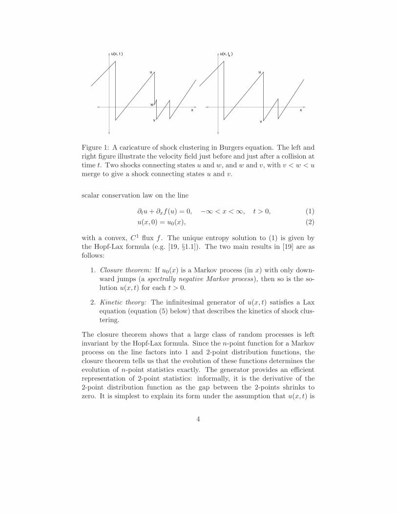
The work presented here bridges this gap. We focus on the macroscopicstatistics of the entropy solution to scalar conservation laws with randominitial data. To fix ideas, consider the problem of determining the statis-tics of the solution to Burgers equation with a random velocity field, suchas Brownian motion or white noise. The initial velocity field immediatelydevelops a profile consisting of infinitely many shocks separated by steeprarefaction waves, which cluster and decay as time increases (see Figure 1).As one may expect, the process of shock clustering is complex (Burgers wasmotivated by turbulence [4]). Nevertheless, for certain classes of randomdata (including Brownian motion and white noise), the evolution of shockstatistics is closed, and in fact, exactly solvable. In recent work, one of theauthors (G.M.) and R. Srinivasan, derived kinetic equations that describethe clustering of shocks for any scalar conservation with convex flux f , and

2

random initial data within a large class [19]. Burgers turbulence is an inter-esting, but particular, instance of this theory.

The combination of the equation-free method and the kinetic theory ofshock clustering can now be explained. Each microscopic state here is aspatial random field – the random velocity field u(x, t)x∈R at any instantin time, and the microscopic interaction is the rapid clustering of manyshocks in a short time frame. The macroscopic statistics are the probabilitydistribution of u(x, t)x∈R (its n-point distribution functions). We comparethe statistics computed via the equation-free scheme with the exact solutionsgiven by the kinetic theory.

Our aims in this work are two-fold: (a) to demonstrate the utility of theequation-free methodology for computing dynamic scaling in shock cluster-ing; (b) to present the exact solutions in shock clustering as a useful bench-mark problem for other practitioners in multiscale methods. For these rea-sons, this paper is organized as follows. We first review the exact solubilityof scalar conservation laws with Markov process initial data, and the kinetictheory of shock clustering in Sections 2.1 and 3.1. We interpret these sys-tems in the context of the equation-free methodology in Sections 2.2 and 3.3.Finally, we turn to a set of numerical experiments that illustrate the methodon a basic test case: the statistics of shocks to Burgers equation with Levyprocess initial data in Section 4. In this case, the kinetic equations of [19]reduce to a basic model of clustering – Smoluchowski’s coagulation equationwith additive kernel. The equation free method provides a new numericalscheme for Smoluchowski’s coagulation equation. This method is shown toaccurately and efficiently compute all self-similar solutions, including thosewith fat tails. Finally, it should be noted that the use of dynamic rescaling inthe method presented here allows us to accurately compute these solutionswith fewer particles in the system – a naive long-time evolution requires aprohibitively large number of particles.

2 Background

2.1 Resolving the closure problem

One of the central obstructions in studies of turbulence (e.g. in homogeneousisotropic turbulence in incompressible fluids) is the closure problem: theevolution equations for n-point statistics involve n + 1-point statistics. Theresults presented in [19] resolve the closure problem for a tractable, butfundamental, class of nonlinear partial differential equations. Consider a

3

v

x

u(x, t )

u

w

+

x

u

v

u(x, t )

Figure 1: A caricature of shock clustering in Burgers equation. The left andright figure illustrate the velocity field just before and just after a collision attime t. Two shocks connecting states u and w, and w and v, with v < w < umerge to give a shock connecting states u and v.

scalar conservation law on the line

∂tu + ∂xf(u) = 0, −∞ < x < ∞, t > 0, (1)

u(x, 0) = u0(x), (2)

with a convex, C1 flux f . The unique entropy solution to (1) is given bythe Hopf-Lax formula (e.g. [19, §1.1]). The two main results in [19] are asfollows:

1. Closure theorem: If u0(x) is a Markov process (in x) with only down-ward jumps (a spectrally negative Markov process), then so is the so-lution u(x, t) for each t > 0.

2. Kinetic theory: The infinitesimal generator of u(x, t) satisfies a Laxequation (equation (5) below) that describes the kinetics of shock clus-tering.

The closure theorem shows that a large class of random processes is leftinvariant by the Hopf-Lax formula. Since the n-point function for a Markovprocess on the line factors into 1 and 2-point distribution functions, theclosure theorem tells us that the evolution of these functions determines theevolution of n-point statistics exactly. The generator provides an efficientrepresentation of 2-point statistics: informally, it is the derivative of the2-point distribution function as the gap between the 2-points shrinks tozero. It is simplest to explain its form under the assumption that u(x, t) is

4

r

u(x, t )

x xl

u

u

l

r

x

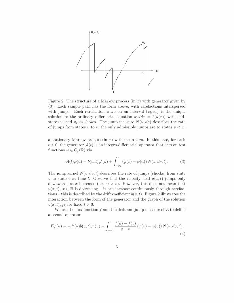
Figure 2: The structure of a Markov process (in x) with generator given by(3). Each sample path has the form above, with rarefactions interspersedwith jumps. Each rarefaction wave on an interval (xl, xr) is the uniquesolution to the ordinary differential equation du/dx = b(u(x)) with end-states ul and ur as shown. The jump measure N(u, dv) describes the rateof jumps from states u to v; the only admissible jumps are to states v < u.

a stationary Markov process (in x) with mean zero. In this case, for eacht > 0, the generator A(t) is an integro-differential operator that acts on testfunctions ϕ ∈ C1

c (R) via

A(t)ϕ(u) = b(u, t)ϕ′(u) +

∫ u

−∞

(ϕ(v) − ϕ(u)) N(u, dv, t). (3)

The jump kernel N(u, dv, t) describes the rate of jumps (shocks) from stateu to state v at time t. Observe that the velocity field u(x, t) jumps onlydownwards as x increases (i.e. u > v). However, this does not mean thatu(x, t), x ∈ R is decreasing – it can increase continuously through rarefac-tions – this is described by the drift coefficient b(u, t). Figure 2 illustrates theinteraction between the form of the generator and the graph of the solutionu(x, t)x∈R for fixed t > 0.

We use the flux function f and the drift and jump measure of A to definea second operator

Bϕ(u) = −f ′(u)b(u, t)ϕ′(u) −∫ u

−∞

f(u) − f(v)

u − v(ϕ(v) − ϕ(u)) N(u, dv, t).

(4)

5

Then the Lax equation derived in [19] is

∂tA = [A,B] = AB − BA. (5)

The compact form of (5) is equivalent to (lengthy, but intuitive) Vlasov-Boltzmann equations for the drift b(u, t) and jump kernel N(u, dv, t) ob-tained by substituting the definitions (3)–(4) in the Lax equation (5) (see [19,equations (26)–(30)]). These are the kinetic equations for shock clustering.

2.2 An equation free approach to shock clustering

The equation-free methodology is applicable to systems with evolution ontwo decoupled scales – fast evolution of microscopic states and slow evolu-tion for macroscopic statistics that describe averages over the microscopicstates. The evolution of the microscopic states is assumed to be known.The evolution of macroscopic statistics is assumed to satisfy a closed equa-tion, but the precise form of this equation is not assumed to be known,and is computationally approximated via a coarse evolver as follows. Themacroscopic statistic at time t is (i) “lifted” into an ensemble of microscopicstates consistent with this macroscopic statistic; (ii) each microscopic statein the ensemble is evolved by the fast evolution over a time step ∆t; (iii)the macroscopic statistic at time t + ∆ is obtained by averaging over theensemble of microscopic states at time t + ∆t.

We now combine the kinetic theory of shock clustering with the equation-free methodology. Assume t > 0 is fixed. A microscopic state is a spatialrandom field u(x, t)x∈R. The microscopic evolution is the clustering of shocksand the decay of rarefactions. The macroscopic statistics are its 1 and 2-point functions. Since the 1 and 2-point functions can be computed onceA(t) is known, an equivalent macroscopic statistic is the generator A(t),and the closed macroscopic evolution is given by the Lax equation (5). This(exact) evolution is contrasted with the computational coarse evolver thatuses only the microscopic evolution of shocks and rarefactions.

Thus, for this particular application, the coarse evolver of the equation-free scheme consists of three steps:

1. Sample P realizations of the Markov process u(x, 0) given its generatorA(0). Call these uj(x, 0), j = 1, . . . , P .

2. Evolve each realization uj in parallel for a short burst of time ∆t bythe PDE (1). This has a simple particle interpretation – the shocksbehave like sticky particles – with a rule of ‘stickiness’ determined byf .

6

3. Estimate the generator A(∆t) from the P realizations uj(x,∆t), j =1, . . . , P . In practice, this is the most difficult step.

At the end of the short time burst, ∆t, we have progressed from A(0) toA(∆t). In general, the time evolution of A(t) may now be accelerated byusing the difference (A(∆t) − A(0))/∆t as an estimate of A at t = 0. Forexample, this estimate can be fed into a forward Euler integration schemewith a time-step ∆T ≫ ∆t.

In the examples treated in this paper, the shocks cluster into larger andlarger shocks as time evolves, and the natural long-time limit to consideris self-similar shock statistics. We use two distinct techniques to acceleratethe time evolution to capture the self-similar solutions. The first is dynamic

renormalization. After time ∆t we suitably rescale A(∆t) before using itas the input to the next step of the microscopic evolver. This approach canonly be used to compute self-similar solutions that are dynamically stable(in rescaled variables). In the second approach, the self-similar solution isreformulated as a coarse fixed point problem. Self-similar solutions are thendetermined via a Newton-GMRES scheme. The advantage of this approachis that the method will converge quadratically (given a sufficiently goodinitial guess) regardless of the stability of the desired self-similar solution.Both these approaches have been explored in previous work by one of theauthors (I.G.K) and his co-workers (see e.g. [11]). The main novelty herelies in the application of these techniques to shock-clustering. In order todescribe the implementation of these ideas, we now describe some exactsolutions to shock clustering in greater detail.

3 Exact solutions: theory and computation

3.1 The Burgers-Levy case

The work [19] builds on two sets of results for Burgers equations: pioneering,but formal, calculations of Duchon and his students [5, 6]; and an importantclosure theorem of Bertoin [2]. It is simplest to describe these results in thefollowing situation.

Consider the entropy solution to Burgers equation on the half-line [0,∞):

∂tu + ∂x

(

u2

2

)

= 0, 0 < x < ∞, t > 0 (6)

u(x, 0) = u0(x) ≤ 0, (7)

where u0(x) is a piecewise constant, decreasing Levy process. (A boundarycondition at 0 is not needed since characteristics only flow out of the domain

7

[0,∞)). In this context, Bertoin’s closure theorem asserts that the processu(x, t)−u(0, t),x ≥ 0 remains a piecewise constant, decreasing Levy processfor each t > 0. Levy processes are Markov processes with increments thatare independent and identically distributed. Consequently, their jump kernelN(u, dv) depends only on the difference u−v. By Bertoin’s theorem, at anyt > 0, the generator A(t) is of the form 1

A(t)ϕ(u) =

∫ ∞

0(ϕ(u − s) − ϕ(u)) f(s, t) ds. (8)

The general Vlasov-Boltzmann equation (5) now simplifies to Smoluchowski’s

coagulation equation with additive kernel :

∂n

∂t(s, t) =

1

2

∫ s

0s n(t, s − s′)n(s′, t)ds′ −

∫ ∞

0(s + s′)n(s, t)n(s′, t)ds′, (9)

where the number density n(s, t) is related to the Levy density f(s, t) by

n(s, t) =f(s, t)

∫ ∞

0 rf(r, t) dr. (10)

We briefly review an intuitive description of the link between (6) and(9) [18, §2.1]. First, note that by restricting attention to piecewise constant,decreasing velocity fields, we have prevented the appearance of any rarefac-tion waves in the system. Let m0(t) =

∫ ∞

0 f(s, t) ds denote the expectednumber of jumps for the Levy process u(x, t) in a unit interval and assumem0(0) < ∞. Then m0(t) ≤ m0(0) < ∞ for each t > 0 since the total num-ber of shocks can only decrease by collisions. For each t ≥ 0, the processu(x, t) − u(0, t) with jump density f(s, t) has the following form:

1. The shock locations 0 = x0(t) < x1(t) < x2(t) < . . . xj(t) < . . . form aPoisson process with rate m0(t).

2. The size of the shocks sj(t) at the jump locations xj(t) are indepen-dent, identically distributed (iid) random variables with probabilitydensity m0(t)

−1f(s, t).

3. The velocity difference u(x, t)−u(0, t) is a piecewise constant functionthat takes the values

uk(x, t) = −k−1∑

j=1

sj, xk−1 < x < xk, k ≥ 1. (11)

1We have assumed that the Levy measure of u(x, t) has a density f(s, t) for convenience.See [18, 2] for the completely general statement

8

In order that such a velocity field constitute a weak solution to (6), thespeed of shocks is given by the Rankine-Hugoniot relation

xk = −k−1∑

j=1

sj −sk

2, (12)

When two shocks meet, they stick and the speed recomputed from theRankine-Hugoniot relation with the new left and right limits. We com-pute the rate of growth and decay of individual shocks by summing over allpossible collision events to obtain (9) (see [18, §2.1] for details).

3.2 Long time asymptotics

The behavior of (9) is well understood [17]. Consider the pth moment

Mp(t) =

∫ ∞

0spn(s, t) ds, (13)

and call M0(t) the total number and M1(t) the total mass 2. Then equation(9) has a unique global solution for any initial measure with M1 < ∞ [17,Thm 2.8] (other moments, including M0 may be infinite). Further, thesolution preserves mass, and without loss of generality, we may rescale theinitial data n0 so that

M1(t) =

∫ ∞

0sn(s, t) ds = 1, t ≥ 0. (14)

For each ρ ∈ (0, 1], equation (9) has a self-similar solution

n(s, t) = e−2t/βnρ(e−t/βs), (15)

where β = ρ/(1 + ρ), and

nρ(s) =1

π

∞∑

k=1

(−1)k−1skβ−2

k!Γ(1 + k − kβ)sin πkβ. (16)

In the case ρ = 1, the formula above simplifies to

n1(s) =e−s/4

√4πs3

. (17)

2This terminology is motivated by the origins of Smoluchowski’s coagulation equationin physical chemistry [8]

9

Each self-similar solution has mass 1. However, they differ in their asymp-totics as s → ∞. Only the solution for ρ = 1 has an exponential tail; foreach 0 < ρ < 1, we find the algebraic decay (“fat tail”)

nρ(s) ∼ρ + 1

|Γ(−ρ)|s−(2+ρ)s → ∞. (18)

As a consequence, for any 0 < ρ < 1, the ρ+ 1-st moment diverges logarith-mically:

∫ s

0r1+ρnρ(r) dr ∼ ρ + 1

|Γ(−ρ)| log s, s → ∞. (19)

All initial densities with M2 < ∞ converge to the self-similar solutionwith ρ = 1. The approach to the fat-tailed self-similar solutions is delicate.Roughly speaking, an initial density n(s, 0) lies in the domain of attractionof nρ if and only if the tails of n(s, 0) diverge in the same manner as (18)(see [17, Thm 7.1] for necessary and sufficient conditions). This analyticalsubtlety is reflected in numerical calculations of self-similar solutions: a typ-ical fixed point method for finding self-similar solutions usually converges ton1(x), not to any of the fat-tailed solutions. Since the divergence in (19) isonly logarithmic, we will impose the condition M1+ρ < ∞ as a “pinning con-dition” in both the dynamic renormalization and Newton-GMRES schemesto compute the fat-tailed self-similar solutions nρ, 0 < ρ < 1.

3.3 Implementing the coarse evolver

As described in Section 2.2, implementation of the equation-free methodrequires an efficient scheme to estimate the jump kernel of a Markov process,given P paths. This estimation problem is considerably simpler for theBurgers-Levy case. In order to understand the issue, imagine approximatingthe initial velocity field u(x, 0) in (2) by a Markov process with M statesv1 < . . . < vM . In this case, the generator AM (0) is an M × M matrix andit is easy to sample N velocity fields uj(x) generated by AM (0). Similarly,it is easy to evolve each random velocity field by (1) using the Hopf-Laxformula, since a convex hull of N points can be computed in O(N log N)steps. Thus, after time ∆t we have P random velocity fields uj(x,∆t), andour task is to form the best estimate of the generator AM (∆t) from thesesamples. In general, the matrix AM (∆t) has O(M2) terms. However, inthe Burgers-Levy case, as a first approximation, the generator is a Toeplitzmatrix with only M terms. Thus, for fixed M , it can be estimated withhigher accuracy even with relatively few realizations (smaller P ). For these

10

reasons, we focus on the Burgers-Levy case in this article. We expect toanalyze the general Lax equation (5) in future work.

We fix a maximal number of particles N0 and a time step ∆t. The coarseevolver in our numerical computation takes the following form.

1. Assume the initial Levy measure has a density f(s, 0) with m1(0) = 1and m0(0) < ∞.

2. Generate the first N0 jumps of a decreasing Levy process u0(x) withjump density f(s, 0). The initial length of the computational domainis L(0) = xN0

.

3. Evolve the Levy process by Burgers equation up to time ∆t. This isdone in one-step, either by the use of the Hopf-Cole formula, or by thesticky particle algorithm of [3]. As noted above, this step involves thecomputation of a convex hull, and requires O(N0 log N0) steps (i.e. itis fast).

4. Let N(∆t) denote the number of particles in the system and let L(∆t) =xN(∆t) − x1(∆t). Compute the empirical Levy measure

f (e)e (s,∆t) ds =

1

L(∆t)N(∆t)

N(∆t)∑

k=1

δsk(∆t)(ds). (20)

This is the coarse evolver for one trial. In fact, P trials can be run in

parallel, and if the empirical Levy density of each of these is f(e)j , we further

average over the P trials to obtain the coarse evolution

f (e)(s,∆t) ds =1

P

P∑

j=1

f(e)j (s,∆t). (21)

In practice, the scheme above has to be modified to streamline the computa-tion. First, we further smooth the empirical density in (21) to simplify thetask of sampling a Levy process with this empirical density when f (e)(·,∆t)is used as input. Second, all the self-similar solutions have divergent totalnumber (i.e.

∫ ∞

0 nρ(s) ds = ∞). The divergence arises from the number of

small clusters (e.g. n1(s) ∼ s−3/2 as s → 0). At each step of the renor-malization, the number m0(∆t) increases. The computation is terminatedwhen m0 crosses a fixed threshold (the maximal number we use is 2× 107).We finally note that the Levy density (8) completely specifies the generatorA(t). Thus, we have demonstrated, as explained in Section 2.2, that thecoarse evolution is a map from A(0) to A(∆t).

11

4 Numerical experiments

4.1 Fixed point equations

In the numerical experiments, we find it more convenient to work with theSmoluchowski density n, which is related to the Levy density f through(10). It is helpful to denote the coarse evolver as follows: the procedure ofSection 3.3 provides a map: n 7→ G(n) for a Smoluchowski density n(s) on(0,∞). This allows us to recognize the self-similar profiles as fixed points ofa suitable map. Explicitly, we use (15) to see that for each ρ, if aρ = e2∆t/β

and bρ = e∆t/β , with β = ρ/(1 + ρ) then

nρ(s) := aρG(nρ(bρs). (22)

These profiles are numerically computed as follows. We start by fixing avalue for the parameter ρ in the range (0, 1]. Given a Smoluchowski densityn with compact support, let Rρ(n) denote the rescaling of n that satisfiesthe pinning conditions3

∫ ∞

0sRρ(n)(s) ds = 1,

∫ ∞

0s1+ρRρ(n)(s) ds = 1. (23)

For each ρ ∈ (0, 1] and a Smoluchowski density n with sufficiently rapiddecay, we define the renormalized mapping

Hρ(n) := RρGRρ. (24)

The mapping Hρ is a synthesis of time evolution and dynamic rescaling.When ρ = 1, the self-similar profile n1(s) is a fixed point of H1; for 0 < ρ < 1,it is not true that nρ = Hρ(nρ). This is because nρ does not have finite1 + ρ-th moment. Nevertheless, this moment is ‘critical’ in terms of theasymptotic relation (19), and the divergence is logarithmic. Thus, since weare restricted to a finite domain in computations, it is natural to seek thefat-tailed solutions as fixed points of Hρ.

We use two strategies to find the fixed point. The first is a direct iterationof the map above. We term this dynamic renormalization. The scheme isas follows. We first fix 0 < ρ ≤ 1 and an initial Smoluchowski density n(0).We then generate a sequence of Smoluchowski densities via the iteration

n(k+1) = Hρ

(

n(k))

. (25)

3See, for example [21] for a broder discussion of the role of such conditions in dynamicscaling.

12

A second method of solving this equation is to use a fixed point algorithm,such as the Newton-GMRES scheme. For any density n we define the resid-ual

r = n −Hρ(n)

and use a Newton iteration to solve this equation for a value of n that yieldsr = 0. In this setting, the combination of the Newton-Raphson methodwith the matrix-free GMRES scheme is particularly advantageous becausethe Jacobian, ∂r/∂n does not need to be computed explicitly. Instead, aseries of “numerical experiments” is used to approximate the Jacobian in aKrylov subspace. In the results that will follow, the Newton iteration schemeis augmented with an Armijo line search to make the iteration scheme morerobust to the choice of initial guess.

Note that neither procedure selects ρ automatically. Further, our choiceof initial conditions is guided by ρ. We use a monodisperse initial conditionfor ρ = 1 (all shocks of initial size 1), and for other ρ we choose the ini-tial condition n(0) = s−(2+ρ). Thus, our approach is certainly guided by a

priori knowledge of the existence of a 1-parameter family of self-similar so-lutions. In fact, earlier numerical schemes for the computation of self-similarsolutions implicitly used the pinning condition M2 = 1, and thus computerexperiments did not reveal the existence of fat-tailed solutions [13]. We viewthis degeneracy as a useful cautionary note for the numerical computation ofself-similar solutions, here and in other problems, even simple model systemssuch as the heat equation on the linear.

4.2 Results

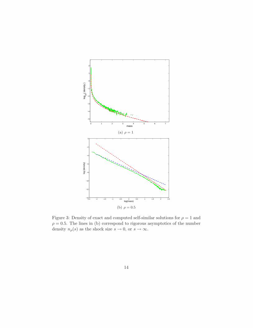
Various representative results of our computations are presented here. In allthe examples below, we denote the exact self-similar solution by nρ and thenumerically computed fixed point by nρ. We first compare the exact andcomputed densities for ρ = 0.5 (fat tails) and ρ = 1 (exponential tails) inFigure 3. Since all densities are rescaled to have unit mass, we define theKolmgorov-Smirnov statistic between computed and exact results:

d(nρ, nρ) = sups≥0

∣

∣

∣Fρ(s) − Fρ(s)

∣

∣

∣,

where

Fρ(s) =

∫ s

0rnρ(r) dr, Fρ(s) =

∫ s

0rnρ(r) dr.

13

0 1 2 3 4 5 6 7

−5

−4

−3

−2

−1

0

1

2

mass

log 10

( de

nsity

)

(a) ρ = 1

−2.5 −2 −1.5 −1 −0.5 0 0.5 1 1.5 2 2.5−14

−12

−10

−8

−6

−4

−2

0

log(mass)

log

(den

sity

)

(b) ρ = 0.5

Figure 3: Density of exact and computed self-similar solutions for ρ = 1 andρ = 0.5. The lines in (b) correspond to rigorous asymptotics of the numberdensity nρ(s) as the shock size s → 0, or s → ∞.

14

0 1 2 3 4 5 6 7 8 9 100

0.2

0.4

0.6

0.8

1

1.2

1.4

mass

first

mom

ent

(a) F1(s) and F1(s)

0 1 2 3 4 5 6 7 8 9 10−7

−6

−5

−4

−3

−2

−1

0

mass

log 10

(er

ror

in fi

rst m

omen

t)

(b) |F1(s) − F1(s)|

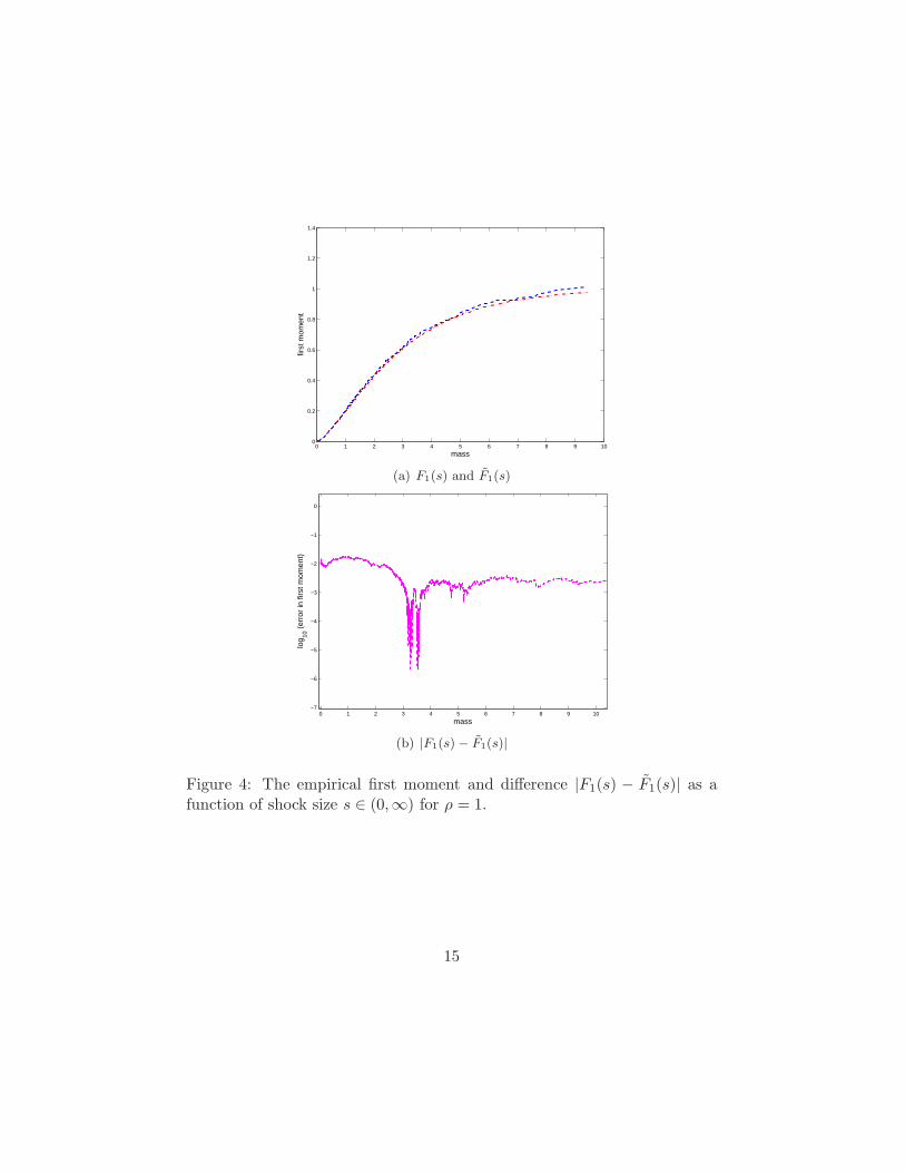
Figure 4: The empirical first moment and difference |F1(s) − F1(s)| as afunction of shock size s ∈ (0,∞) for ρ = 1.

15

0 10 20 30 40 50 60−6

−5

−4

−3

−2

−1

0

mass

log 10

(er

ror

in fi

rst m

omen

t)

ρ=.1

ρ=.2

ρ=.3

ρ=.4

ρ=.5

ρ=.6

ρ=.7

ρ=.8

ρ=.9

(a) Dynamic renormalization

0 0.5 1 1.5 2 2.5 3 3.5 4 4.5 5−4.5

−4

−3.5

−3

−2.5

−2

−1.5

−1

−0.5

mass

log 10

(err

or in

firs

t mom

ent)

ρ=0.1

ρ=0.2

ρ=0.3

ρ=0.4

ρ=0.5

ρ=0.6

ρ=0.7

ρ=0.8

ρ=0.9

(b) GMRES-Newton

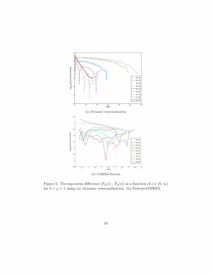
Figure 5: The sup-norm difference |Fρ(s)− Fρ(s)| as a function of s ∈ (0,∞)for 0 < ρ < 1 using (a) dynamic renormalization; (b) Newton-GMRES.

16

The comparison between F1 and F1 is shown in Figure 4. Similar compar-isons for a range of fat-tailed solutions are shown in Figure 5. The numericalcomputation of the exact solutions requires some care. We use the fact thatthey can be written as the density of Levy-stable laws with a nonlinearrescaling (see [17]). A numerical method for computing these densities maybe found in [20]. For higher ρ, the error in the tails is negligible, showingthat both the exact and computed density decay fast. However, the errornear s = 0 can be high (between 20% and 30% in the worst case observed),but it decays rapidly with s for all ρ ∈ (0, 1). This error is caused by thesingularity near s = 0 of the exact solutions nρ, 0 < ρ < 1. It is importantto note however that the convergence of the scheme could be seen withouta priori knowledge of the exact solutions. The initial number of particleswas O(103), and the computation was terminated when the number of par-ticles reached a maximal number 2 × 107 (fixed a priori). At each step ofthe dynamic renormalization, the number of particles must increase sincethe total number of particles is divergent for each of the exact solutions nρ.While our numerical scheme could be adapted to provide higher resolution(e.g. by incorporating special basis functions at s = 0 and near s = ∞to account for divergences), we have refrained from doing so, in order todemonstrate the robust convergence of the scheme used here. As noted atthe end of Section 1 the use of dynamic rescaling was critical for an accuratecomputation of self-similar solutions without a prohibitely large number ofparticles.

5 Discussion

Scalar conservation laws (1)–(2), have played an important role in the de-velopment of the modern theory of nonlinear partial differential equations.These equations illustrate important themes such as singularity formation,non-uniqueness of weak solutions, and the role of entropy conditions thatrestore the uniqueness of solutions. A complete well-posedness theory forthese equations was established in the 1950s by Hopf, Lax and Oleinik (seee.g.[7]). However, neither Burgers nor Hopf viewed the analysis of scalarconservation laws as an end in itself. Instead, their primary interest lay inthe use of these equations as a stepping stone to a fuller understanding ofturbulence (see e.g. [9, 22]). Burgers introduced his model equation in the1930’s to study turbulence and spent much of his career exploring the evo-lution of random initial data [4]. Similarly, Hopf was the first to preciselyformulate an evolution equation for the probability distribution of solutions

17

to the Navier-Stokes equations [10].We know today that the study of Burgers equation, or other scalar con-

servation laws, with random initial data does not capture the essential mech-anisms of isotropic homogeneous turbulence in incompressible fluids. Never-theless, it does serve as a concrete model for one aspect of turbulence – thepropagation of randomness by a deterministic dynamical system. The re-sults summarized in Section 2.1 reflect an unexpected exact solvability of theevolution of shock statistics for large classes of random initial data. Muchas the Hopf-Lax formula for scalar conservation laws serves as a basic modelto convey insight into nonlinear partial differential equations, it is our viewthat the exact solvability for the evolution of random data, can be used tocommunicate many basic ideas in the modeling of complex stochastic sys-tems. The main thrust of this article has been to demonstrate the utility ofthese exact solutions in the study of equation free methods.

Within the context of this class of problems, we have only explored thesimplest class of exact solutions – the solution to Burgers equation with Levyprocess initial data. It remains to explore other “non-Burgers” flux functions(i.e. f(u) 6= u2/2), as well as other classes of random initial processes suchas white noise, or Markov process initial data. The clustering processesthat emerge from these data are more complex (compare the full kineticequations [19, Equations (27)–(30)] with equation(9)). The main challengein applying the equation free scheme to these exact solutions lies in the“projection step” (i.e. step 4 in the scheme outlined in Section 2.2). In thispaper, this task reduces to estimating the Levy measure of a Levy processgiven many samples of the process. As noted in Section 2.1, Levy processesare Markov processes whose jump measure N(u, dv) depends only on thedifference u−v. For general f(u) and for white noise data, this simplificationdoes not hold – that is, one has to estimate a jump kernel N(u, dv) thatdepends on two variables, not one. This changes the complexity of theproblem substantially, and remains a challenge for future work.

More broadly, Burgers equation and scalar conservation laws, continueto play an important role in stochastic modeling. Our work provides anexample of uncertainty quantification – the exact evolution of an initialprobability distribution is compared with a numerically computed evolution.Our work could also be contrasted with other uses of Burgers equation instochastic modeling. For instance, Majda, Turkington and their co-workershave explored the use of truncations of the Burgers equation to coarse-grain invariant measures. In contrast with their work, our work includes notruncation of the underlying partial differential equation, nor does it involvea projection of a non-Gaussian probability distribution onto Gaussians [12,

18

15]. The fundamental dynamics here are the interactions of shocks, not theevolution of low-modes, whereas the goal in [12, 15] is to approximate thetransport of energy to high, unresolved modes, by a slowly-varying Gaussiancorrection of the energy in low-modes. These works explore complementaryphysical regimes, and it is of interest to understand the common featuresand differences between them.

6 Acknowledgements

One of the authors (I.G.K.) would like to remember here Stephen A. Orszag,who suggested this very problem as a challenge for equation free methods adecade ago.

The authors also acknowledge support from the following funding agen-cies. M.O.W. acknowledges support from NSF DMS 1204783. I.G.K. ac-knowledges partial support from US-AFOSR through grant number FA9550-12-1-0332 and NSF grant CDSE 1310173. G.M. acknowledges partial sup-port from NSF DMS 1411278.

References

[1] F. J. Alexander, G. Johnson, G. L. Eyink, and I. G.

Kevrekidis, Equation-free implementation of statistical moment clo-

sures, Phys. Rev. E (3), 77 (2008), pp. 026701, 7.

[2] J. Bertoin, The inviscid Burgers equation with Brownian initial ve-

locity, Commun. Math. Phys., 193 (1998), pp. 397–406.

[3] Y. Brenier and E. Grenier, Sticky particles and scalar conservation

laws, SIAM J. Numer. Anal., 35 (1998), pp. 2317–2328 (electronic).

[4] J. M. Burgers, The nonlinear diffusion equation, Dordrecht: Reidel,1974.

[5] L. Carraro and J. Duchon, Equation de Burgers avec conditions

initiales a accroissements independants et homogenes, Ann. Inst. H.Poincare Anal. Non Lineaire, 15 (1998), pp. 431–458.

[6] M.-L. Chabanol and J. Duchon, Markovian solutions of inviscid

Burgers equation, J. Stat. Phys., 114 (2004), pp. 525–534.

[7] C. M. Dafermos, Hyperbolic conservation laws in continuum physics,Springer-Verlag, New York, 2000.

19

[8] R. L. Drake, A general mathematical survey of the coagulation equa-

tion, in Topics in Current Aerosol Research, G. M. Hidy and J. R.Brock, eds., no. 2 in International reviews in Aerosol Physics and Chem-istry, Pergammon, 1972, pp. 201–376.

[9] E. Hopf, The partial differential equation ut + uux = µxx, Commun.Pure Appl. Math., 3 (1950), pp. 201–230.

[10] , Statistical hydromechanics and functional calculus, J. RationalMech. Anal., 1 (1952), pp. 87–123.

[11] D. A. Kessler, I. G. Kevrekidis, and L. Chen, Equation-free dy-

namic renormalization of a Kardar-Parisi-Zhang-type equation, Physi-cal Review E, 73 (2006), p. 036703.

[12] R. Kleeman and B. E. Turkington, A nonequilibrium statistical

model of spectrally truncated Burgers-Hopf dynamics, Communicationson Pure and Applied Mathematics, 67 (2014), pp. 1905–1946.

[13] M. H. Lee, A survey of numerical solutions to the coagulation equation,Journal of Physics A: Mathematical and General, 34 (2001), p. 10219.

[14] J. Li, P. G. Kevrekidis, C. W. Gear, and I. G. Kevrekidis,Deciding the nature of the coarse equation through microscopic simula-

tions: the baby-bathwater scheme, SIAM Rev., 49 (2007), pp. 469–487(electronic).

[15] A. J. Majda and I. Timofeyev, Remarkable statistical behavior

for truncated Burgers–Hopf dynamics, Proceedings of the NationalAcademy of Sciences, 97 (2000), pp. 12413–12417.

[16] G. Menon, Complete integrability of shock clustering and Burgers tur-

bulence, Arch. Ration. Mech. Anal., 203 (2012), pp. 853–882.

[17] G. Menon and R. L. Pego, Approach to self-similarity in Smolu-

chowski’s coagulation equations, Comm. Pure Appl. Math., 57 (2004),pp. 1197–1232.

[18] G. Menon and R. L. Pego, Universality classes in Burgers turbu-

lence, Comm. Math. Phys., 273 (2007), pp. 177–202.

[19] G. Menon and R. Srinivasan, Kinetic theory and Lax equations

for shock clustering and Burgers turbulence, J. Stat. Phys., 140 (2010),pp. 1195–1223.

20

[20] J. P. Nolan, Numerical calculation of stable densities and distribution

functions, Communications in statistics. Stochastic models, 13 (1997),pp. 759–774.

[21] C. W. Rowley, I. G. Kevrekidis, J. E. Marsden, and K. Lust,Reduction and reconstruction for self-similar dynamical systems, Non-linearity, 16 (2003), p. 1257.

[22] J. von Neumann, Recent theories of turbulence, in Collected works.Vol. VI: Theory of games, astrophysics, hydrodynamics and meteorol-ogy, T. editor, ed., The Macmillan Co., New York, 1963.

21