efficient modeling, simulation and coarse-graining of ... modeling, simulation and coarse-graining...

Nature Methods

Efficient modeling, simulation and coarse-graining of biological complexity with NFsim Michael W Sneddon, James R Faeder & Thierry Emonet Supplementary File Title Supplementary Figure 1 Validation of NFsim output with a simple enzymatic reaction system. Supplementary Figure 2 Schematic diagram of the trivalent-ligand, bivalent-receptor (TLBR)

model. Supplementary Figure 3 Validation of NFsim output with the TLBR model. Supplementary Figure 4 Validation of the NFsim model of steady-state actin assembly and

severing. Supplementary Figure 5 Validation of the NFsim model of chemoreceptor adaptation. Supplementary Figure 6 Performance and memory scaling tests with the TLBR model. Supplementary Figure 7 Experimental validation of the TLBR model. Supplementary Table 1 Normalized runtime performance of NFsim vs. DYNSTOC,

RuleMonkey, and Kappa. Supplementary Table 2 Names and descriptors of the compendium of FcεRI signaling models

used in performance tests. Supplementary Table 3 Summary of bulk monomer concentrations used in the steady-state

actin assembly, branching and severing model. Supplementary Table 4 Spontaneous actin assembly and depolymerization parameters used in

the steady-state actin assembly, branching and severing model. Supplementary Table 5 Arp2/3 and VCA mediated branching parameters used in the steady-

state actin assembly, branching and severing model. Supplementary Table 6 Actin hydrolysis, phosphate release, and ADF/cofilin severing

parameters used in the steady-state actin assembly, branching and severing model.

Supplementary Table 7 Capping Protein reaction parameters used in the steady-state actin assembly, branching and severing model.

Supplementary Note 1 Overview of rule-based modeling. Supplementary Note 2 Overview of constructing NFsim models with the BioNetGen

Language. Supplementary Note 3 Detailed comparison to StochSim / DYNSTOC / RuleMonkey / Kappa. Supplementary Note 4 Simple enzymatic system validation. Supplementary Note 5 Trivalent-ligand, bivalent-receptor (TLBR) validation and

performance. Supplementary Note 6 TLBR parameter scanning and estimation. Supplementary Note 7 Multisite phosphorylation model. Supplementary Note 8 Compendium of early FcεRI signaling models. Supplementary Note 9 Actin assembly, branching and severing models. Supplementary Note 10 Model of bacterial chemoreceptor adaptation. Supplementary Note 11 Coarse-grained model of the bacterial flagellar motor. Supplementary Note 12 Negative feedback oscillator model. Note: Supplementary Videos 1 and 2 are available on the Nature Methods website.

Nature Methods: doi: 10.1038/nmeth.1546

1

Supplementary Figures

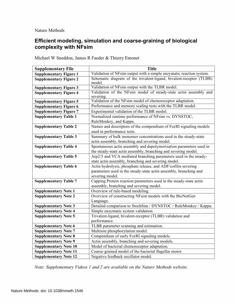
Supplementary Figure 1 | Validation of NFsim output with a simple enzymatic reaction system

(a) Mean number and (b) standard deviation of the molecular species Sp (blue circles) and S (red squares) of 3000

NFsim simulation runs of the simple push-pull enzymatic system compared to an equivalent set of BioNetGen SSA

simulations (black lines). For details of the enzymatic system, see Supplementary Note 4.


2

Supplementary Figure 2 | Schematic diagram of the trivalent-ligand, bivalent-receptor (TLBR) model

(a) In the TLBR model, membrane-bound receptors have two binding sites for a trivalent ligand molecule.

Receptors can be cross-linked by mutual binding to a single ligand. (b) The system can be represented with a free-

binding rule, a crosslinking rule and an unbinding rule. The blue object represents a ligand molecule with three

binding sites and the square objects represent a receptor with two ligand binding sites. Filled black circles are

binding sites that are occupied, open black circles are binding sites that are available, and a lack of any circle

represents sites that can be either bound or occupied. (c) Aggregation of receptors and ligands leads to a nearly

infinite reaction network composed of an enormous number of chemical species. This figure is adapted with

permission from Supplementary Ref. 40

. See Supplementary Note 5 for more details of the TLBR model.


3

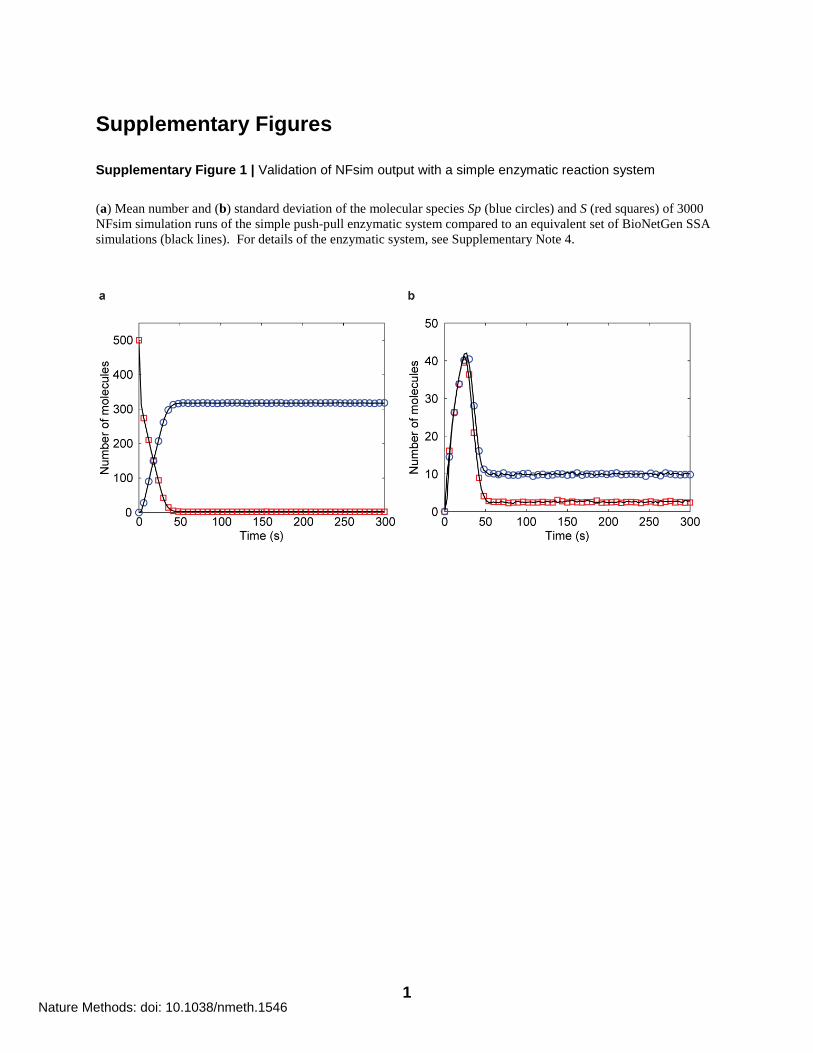
Supplementary Figure 3 | Validation of NFsim output with the TLBR model

(a) Trajectories of the TLBR simulation averaged over 40 trials for two different parameter sets in NFsim (blue

circles, red squares) plotted against the output of a problem-specific TLBR simulator (black lines) 40

. The peaking

trajectory (blue circles) parameters are: 50000totL , 3000totR , 2.7totc , 16.8 , and 0.01offk , where

/X tot offk R k and 13 /tot tot offc k L k . The ramping trajectory (red squares) parameters are: 2000totL , 3000totR ,

0.11totc , 16.8 , and 0.01offk . (b) The fraction of receptors connected to an aggregate of a particular size can

be computed analytically in steady-state41

. We compare the distribution of receptors in NFsim in two cases (blue

circles, red squares) to the analytic solution (black lines). The parameters for the first case (red squares) are:

42000totL , 3000totR , 0.378totc , 0.3 , and 0.01offk . The parameters for the second case (blue circles) are:

2000totL , 3000totR , 0.054totc , 16.8 , and 0.01offk . See Supplementary Note 5 for more details of the TLBR

model and simulations.


4

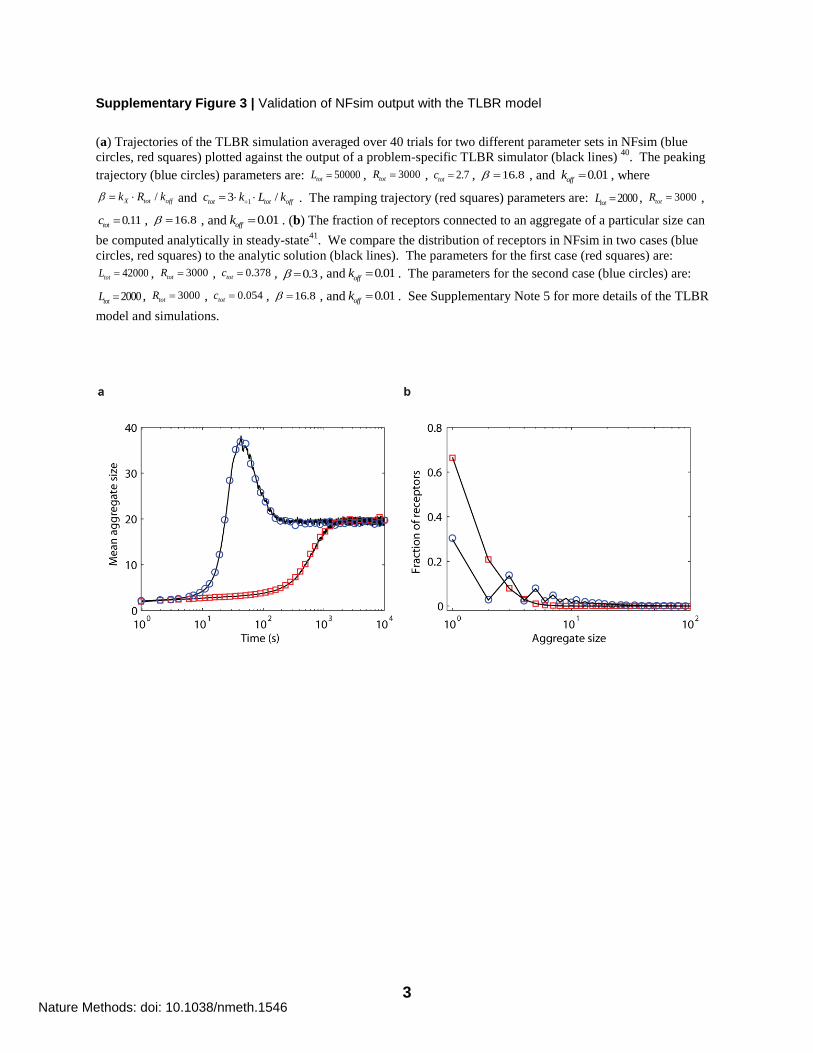
Supplementary Figure 4 | Validation of the NFsim model of steady-state actin assembly and severing

This model implemented in NFsim was originally described in Supplementary Ref. 42

. See Supplementary Note 9

for more details of this model. (a) The steady-state probability distribution of actin filament lengths for varying

concentrations of ADF/cofilin. The probability distribution is computed over 10,000 second simulations. Compare

to Figure 2C of the original study42

. (b) The length of a single actin filament as a function of time for varying

concentrations of ADF/cofilin. Compare to Figure 2B of the original study42

. Results assume that 330 actin

subunits correspond to 1m in filament length, as in the original study.


5

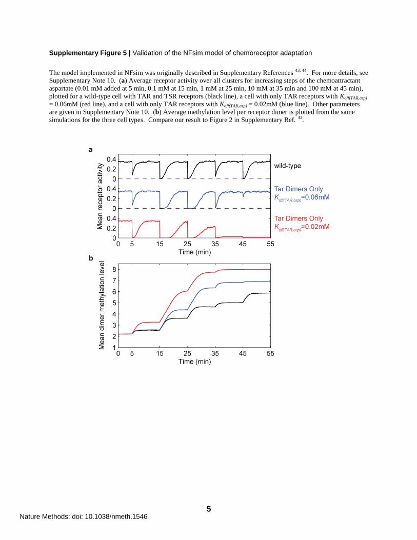
Supplementary Figure 5 | Validation of the NFsim model of chemoreceptor adaptation

The model implemented in NFsim was originally described in Supplementary References 43, 44

. For more details, see

Supplementary Note 10. (a) Average receptor activity over all clusters for increasing steps of the chemoattractant

aspartate (0.01 mM added at 5 min, 0.1 mM at 15 min, 1 mM at 25 min, 10 mM at 35 min and 100 mM at 45 min),

plotted for a wild-type cell with TAR and TSR receptors (black line), a cell with only TAR receptors with Koff(TAR,asp)

= 0.06mM (red line), and a cell with only TAR receptors with Koff(TAR,asp) = 0.02mM (blue line). Other parameters

are given in Supplementary Note 10. (b) Average methylation level per receptor dimer is plotted from the same

simulations for the three cell types. Compare our result to Figure 2 in Supplementary Ref. 43

.


6

Supplementary Figure 6 | Performance and memory scaling tests with the TLBR model

(a) Performance scaling of NFsim with increasing reaction network size allowing ring formation in aggregates (red

squares), prohibiting ring formation in aggregates (blue circles), and compared to an “on-the-fly” SSA (black

circles). The phase transition between mostly free receptors (solution phase) and mostly aggregated receptors (sol-

gel phase) occurs when 4 as indicated by the dashed black line. Parameters for these simulations are: 42000totL ,

3000totR , 0.84totc , and 0.01offk . (b) NFsim performance scaling (blue circles, left axis) and memory scaling

(green triangles, right axis) with increasing numbers of molecules simulated with the TLBR system allowing ring

formation. Simulation parameters are: (1 0.067)totL T , 0.067totR T , 0.84totc , 90 , and 0.01offk , where T is

the total number of molecules. See Supplementary Note 5 for additional details.


7

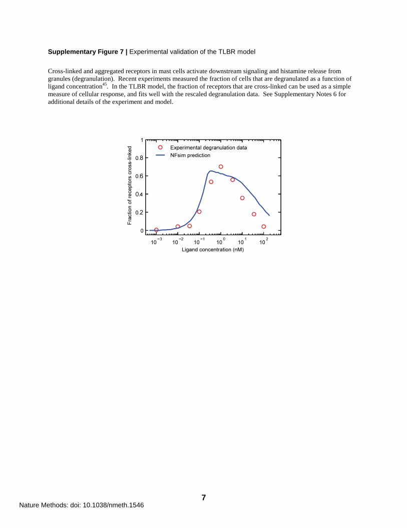
Supplementary Figure 7 | Experimental validation of the TLBR model

Cross-linked and aggregated receptors in mast cells activate downstream signaling and histamine release from

granules (degranulation). Recent experiments measured the fraction of cells that are degranulated as a function of

ligand concentration45

. In the TLBR model, the fraction of receptors that are cross-linked can be used as a simple

measure of cellular response, and fits well with the rescaled degranulation data. See Supplementary Notes 6 for

additional details of the experiment and model.


8

Supplementary Tables

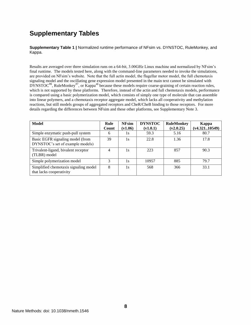
Supplementary Table 1 | Normalized runtime performance of NFsim vs. DYNSTOC, RuleMonkey, and Kappa.

Results are averaged over three simulation runs on a 64-bit, 3.00GHz Linux machine and normalized by NFsim‟s

final runtime. The models tested here, along with the command-line parameters needed to invoke the simulations,

are provided on NFsim‟s website. Note that the full actin model, the flagellar motor model, the full chemotaxis

signaling model and the oscillating gene expression model presented in the main text cannot be simulated with

DYNSTOC46

, RuleMonkey47

, or Kappa48

because these models require coarse-graining of certain reaction rules,

which is not supported by these platforms. Therefore, instead of the actin and full chemotaxis models, performance

is compared using a basic polymerization model, which consists of simply one type of molecule that can assemble

into linear polymers, and a chemotaxis receptor aggregate model, which lacks all cooperativity and methylation

reactions, but still models groups of aggregated receptors and CheR/CheB binding to those receptors. For more

details regarding the differences between NFsim and these other platforms, see Supplementary Note 3.

Model Rule

Count

NFsim

(v1.06)

DYNSTOC

(v1.0.1)

RuleMonkey

(v2.0.25)

Kappa

(v4.321..10549)

Simple enzymatic push-pull system 6 1s 59.3 5.16 80.7

Basic EGFR signaling model (from

DYNSTOC‟s set of example models)

39 1s 22.8 1.36 17.8

Trivalent-ligand, bivalent receptor

(TLBR) model

4 1s 223 857 90.3

Simple polymerization model 3 1s 10957 885 79.7

Simplified chemotaxis signaling model

that lacks cooperativity

8 1s 568 366 33.1


9

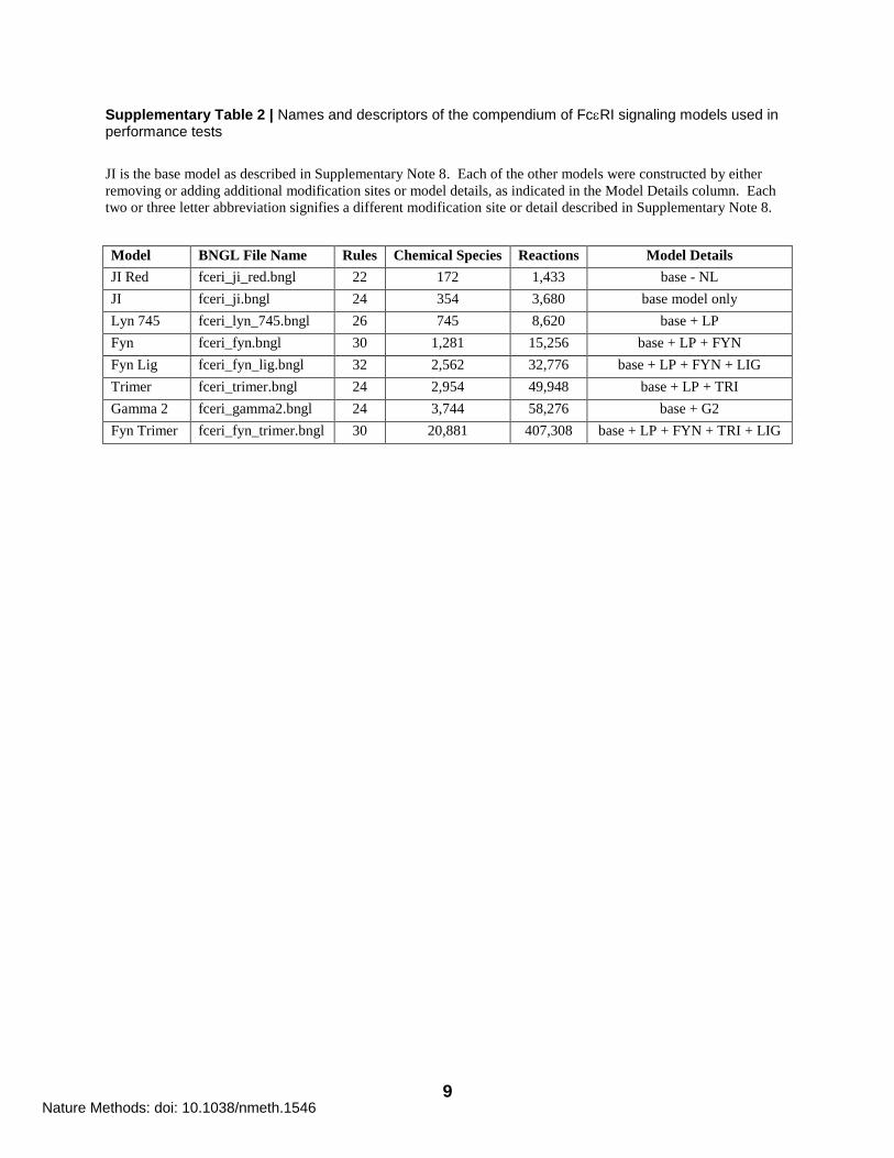
Supplementary Table 2 | Names and descriptors of the compendium of FcRI signaling models used in performance tests

JI is the base model as described in Supplementary Note 8. Each of the other models were constructed by either

removing or adding additional modification sites or model details, as indicated in the Model Details column. Each

two or three letter abbreviation signifies a different modification site or detail described in Supplementary Note 8.

Model BNGL File Name Rules Chemical Species Reactions Model Details

JI Red fceri_ji_red.bngl 22 172 1,433 base - NL

JI fceri_ji.bngl 24 354 3,680 base model only

Lyn 745 fceri_lyn_745.bngl 26 745 8,620 base + LP

Fyn fceri_fyn.bngl 30 1,281 15,256 base + LP + FYN

Fyn Lig fceri_fyn_lig.bngl 32 2,562 32,776 base + LP + FYN + LIG

Trimer fceri_trimer.bngl 24 2,954 49,948 base + LP + TRI

Gamma 2 fceri_gamma2.bngl 24 3,744 58,276 base + G2

Fyn Trimer fceri_fyn_trimer.bngl 30 20,881 407,308 base + LP + FYN + TRI + LIG


10

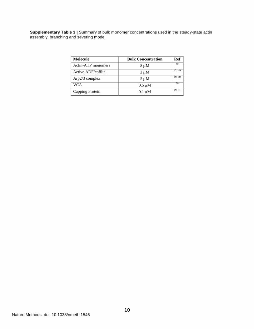
Supplementary Table 3 | Summary of bulk monomer concentrations used in the steady-state actin assembly, branching and severing model

Molecule Bulk Concentration Ref

Actin-ATP monomers 8 M 49

Active ADF/cofilin 2 M 42, 49

Arp2/3 complex 5 M 49, 50

VCA 0.5 M 50

Capping Protein 0.1 M 49, 51


11

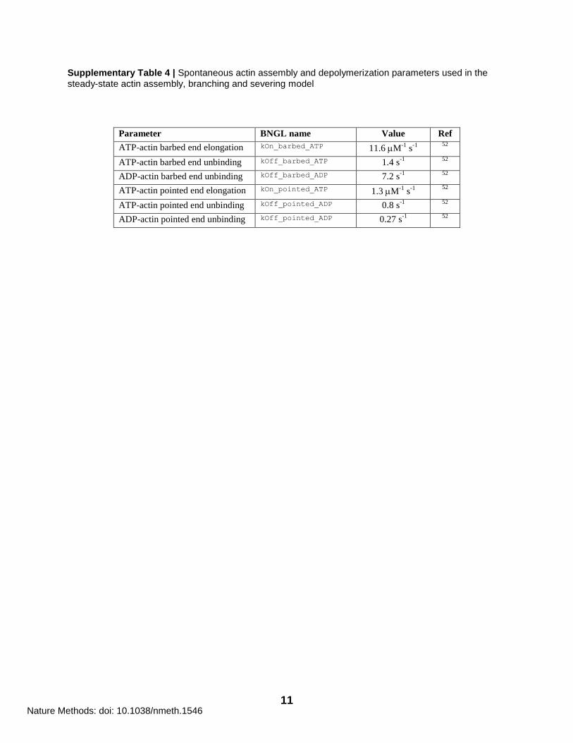
Supplementary Table 4 | Spontaneous actin assembly and depolymerization parameters used in the steady-state actin assembly, branching and severing model

Parameter BNGL name Value Ref

ATP-actin barbed end elongation kOn_barbed_ATP 11.6 M-1

s-1

52

ATP-actin barbed end unbinding kOff_barbed_ATP 1.4 s-1

52

ADP-actin barbed end unbinding kOff_barbed_ADP 7.2 s-1

52

ATP-actin pointed end elongation kOn_pointed_ATP 1.3 M-1

s-1

52

ATP-actin pointed end unbinding kOff_pointed_ADP 0.8 s-1

52

ADP-actin pointed end unbinding kOff_pointed_ADP 0.27 s-1

52


12

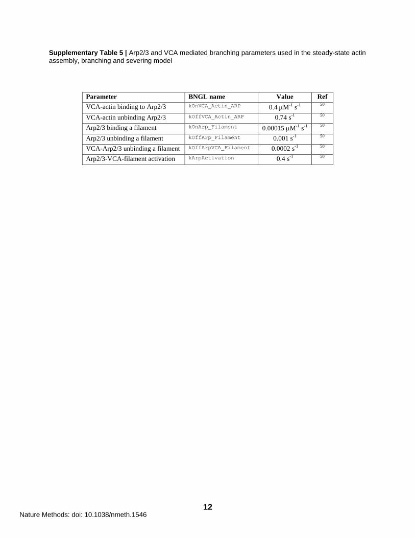
Supplementary Table 5 | Arp2/3 and VCA mediated branching parameters used in the steady-state actin assembly, branching and severing model


VCA-actin binding to Arp2/3 kOnVCA_Actin_ARP 0.4 M-1

s-1

50

VCA-actin unbinding Arp2/3 kOffVCA_Actin_ARP 0.74 s-1

50

Arp2/3 binding a filament kOnArp_Filament 0.00015 M-1

s-1

50

Arp2/3 unbinding a filament kOffArp_Filament 0.001 s-1

50

VCA-Arp2/3 unbinding a filament kOffArpVCA_Filament 0.0002 s-1

50

Arp2/3-VCA-filament activation kArpActivation 0.4 s-1

50


13

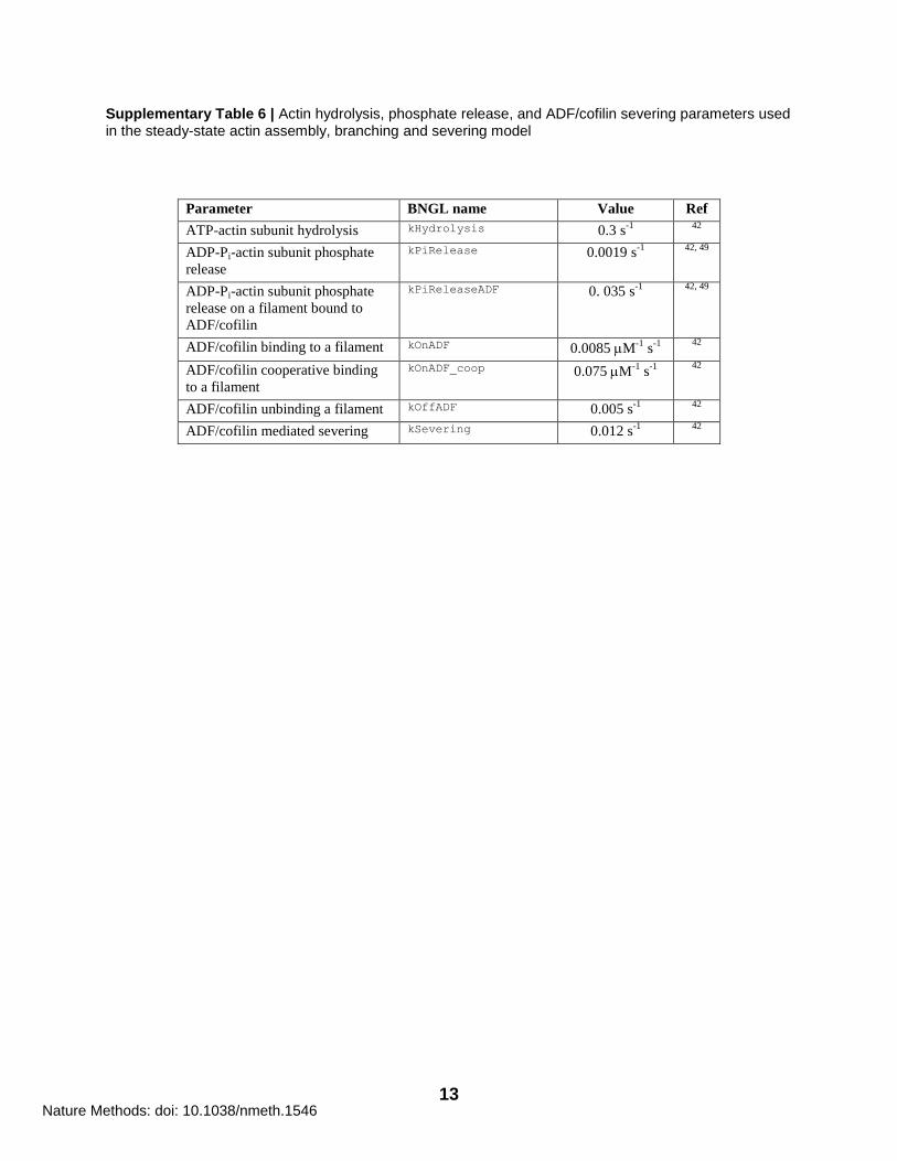
Supplementary Table 6 | Actin hydrolysis, phosphate release, and ADF/cofilin severing parameters used in the steady-state actin assembly, branching and severing model


ATP-actin subunit hydrolysis kHydrolysis 0.3 s-1

42

ADP-Pi-actin subunit phosphate

release

kPiRelease 0.0019 s-1

42, 49

ADP-Pi-actin subunit phosphate

release on a filament bound to

ADF/cofilin

kPiReleaseADF 0. 035 s-1

42, 49

ADF/cofilin binding to a filament kOnADF 0.0085 M-1

s-1

42

ADF/cofilin cooperative binding

to a filament

kOnADF_coop 0.075 M-1

s-1

42

ADF/cofilin unbinding a filament kOffADF 0.005 s-1

42

ADF/cofilin mediated severing kSevering 0.012 s-1

42


14

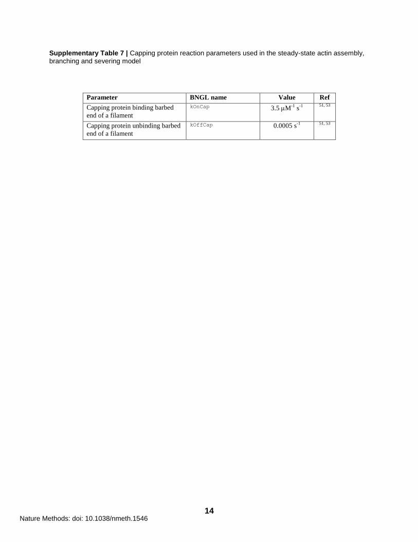
Supplementary Table 7 | Capping protein reaction parameters used in the steady-state actin assembly, branching and severing model


Capping protein binding barbed

end of a filament

kOnCap 3.5 M-1

s-1

51, 53

Capping protein unbinding barbed

end of a filament

kOffCap 0.0005 s-1

51, 53


15

Supplementary Notes

In these Supplementary notes, we provide a brief introduction to rule-based modeling, an introduction to building

models in NFsim, an extended comparison to existing rule-based simulators, additional validation / performance

results and additional details of the models mentioned in the main text. The model specification files written in the

BioNetGen Language are available from the NFsim website: http://www.nfsim.org.

1) Overview of rule-based modeling ............................................................................. 16

2) Overview of constructing NFsim models with the BioNetGen Language ................. 17

3) Detailed comparison to StochSim / DYNSTOC / RuleMonkey / Kappa ................... 21

4) Simple enzymatic system validation ......................................................................... 23

5) Trivalent-ligand, bivalent-receptor (TLBR) validation and performance .................. 24

6) TLBR parameter scanning and estimation ............................................................... 25

7) Multisite phosphorylation model ............................................................................... 26

8) Compendium of early FcRI signaling models.......................................................... 27

9) Actin assembly, branching and severing models ..................................................... 28

10) Model of bacterial chemoreceptor adaptation........................................................... 30

11) Coarse-grained model of the bacterial flagellar motor .............................................. 31

12) Negative feedback oscillator model .......................................................................... 32

Supplementary references ...................................................................................................... 33


http://emonet.biology.yale.edu/nfsim

16

Supplementary Note 1 | Overview of rule-based modeling

In organic chemistry diagrams are commonly used to represent chemical structures and to rationalize or

predict complex reaction mechanisms. The diagrammatic representations used by organic chemists typically focus

on only the key atoms in a chemical structure that participate in a reaction, sometimes called the reaction center,

while hiding from view other parts of the structure that don‟t affect reactivity. Protein molecules exhibit a similar

degree of modularity in their reactivity to their smaller organic counterparts, and yet, until relatively recently, a

comparable shorthand notation for describing interactions among proteins was unavailable. Signaling proteins are

composed of multiple components with distinct functionality, which gives rise to the phenomenon of combinatorial

complexity, which we have discussed in the main text. Rule-based modeling languages, such as the BioNetGen

Language (BNGL)54

and Kappa48

, provide a concise yet flexible way for representing the modular composition of

proteins that is analogous to chemical structures used by chemists. The basic elements of a rule-based model, called

molecules in BNGL and agents in Kappa, are structured objects whose components represent functional units of a

protein or other signaling molecule. Components may bind components of other molecules and may also have

internal states that represent different structural conformations or post-translation modifications, such as

phosphorylation. In this way the complete state of a protein either alone or in complex with other proteins may be

represented. This removes a major element of arbitrariness in the naming of chemical species in complex reaction

networks. Each species in a rule-based model specifies exactly the conformational or post-translational modification

state of each component and the complete connectivity of the complex at the component level.

Rules describe the reactions that create and destroy bonds between molecules or that change internal states

of components. Rules may also prescribe synthesis, degradation, or transport of molecules and their complexes.

Just like in organic chemistry, rules specify only the molecules and components that are required for the reaction to

take place, called the reaction context, and the molecules and components that are modified by the reaction, called

the reaction center. For complex proteins, rules typically involve only a small subset of the total number of

components of each reacting molecule. Thus, the enormous combinatorial complexity inherent in such reactions

may be neatly avoided via the rule-based modeling approach. By encoding both a transformation and the known (or

hypothesized) context under which that transformation occurs, rules provide a compact representation of

biochemical knowledge. In the next section we will introduce the syntax of one rule-based modeling language, the

BioNetGen Language, which is used in the specification of NFsim models, and provide a number of specific

examples of how molecules and rules are encoded.


17

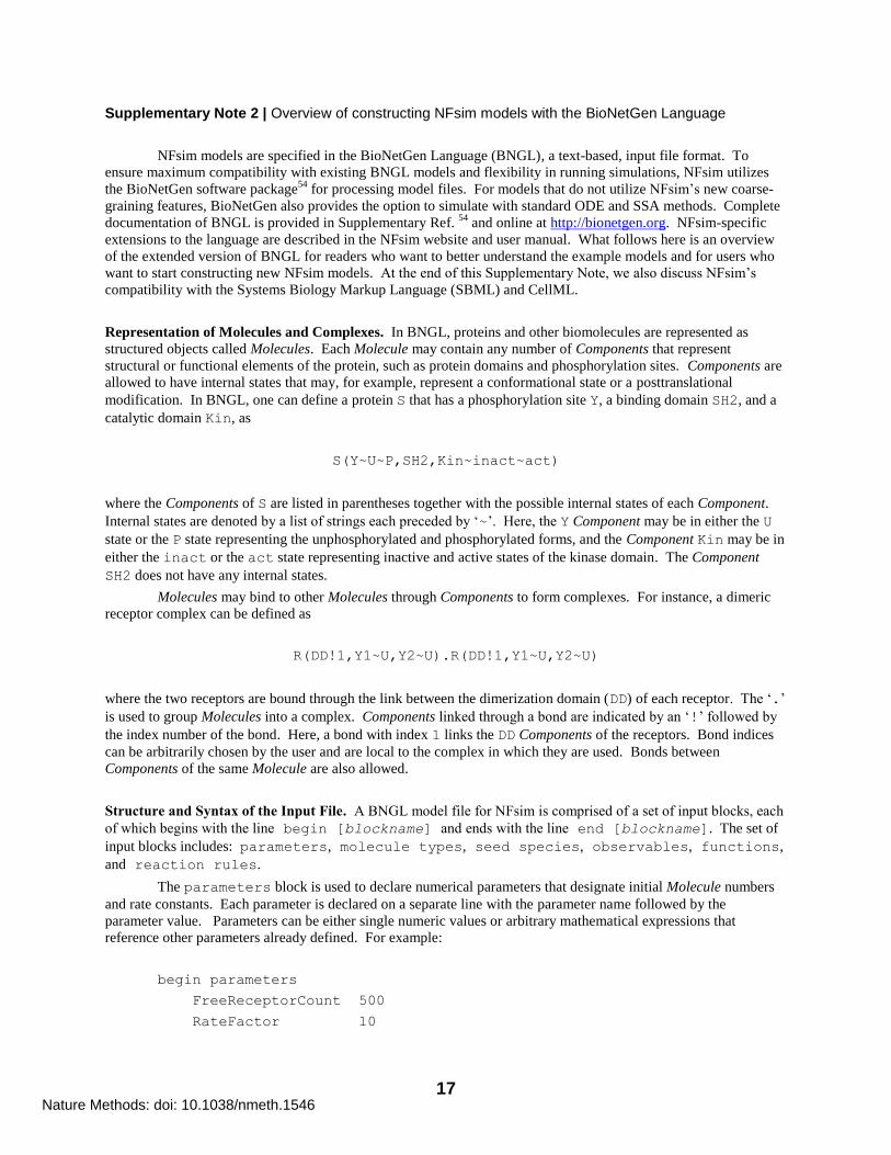
Supplementary Note 2 | Overview of constructing NFsim models with the BioNetGen Language

NFsim models are specified in the BioNetGen Language (BNGL), a text-based, input file format. To

ensure maximum compatibility with existing BNGL models and flexibility in running simulations, NFsim utilizes

the BioNetGen software package54

for processing model files. For models that do not utilize NFsim‟s new coarse-

graining features, BioNetGen also provides the option to simulate with standard ODE and SSA methods. Complete

documentation of BNGL is provided in Supplementary Ref. 54

and online at http://bionetgen.org. NFsim-specific

extensions to the language are described in the NFsim website and user manual. What follows here is an overview

of the extended version of BNGL for readers who want to better understand the example models and for users who

want to start constructing new NFsim models. At the end of this Supplementary Note, we also discuss NFsim‟s

compatibility with the Systems Biology Markup Language (SBML) and CellML.

Representation of Molecules and Complexes. In BNGL, proteins and other biomolecules are represented as

structured objects called Molecules. Each Molecule may contain any number of Components that represent

structural or functional elements of the protein, such as protein domains and phosphorylation sites. Components are

allowed to have internal states that may, for example, represent a conformational state or a posttranslational

modification. In BNGL, one can define a protein S that has a phosphorylation site Y, a binding domain SH2, and a

catalytic domain Kin, as

S(Y~U~P,SH2,Kin~inact~act)

where the Components of S are listed in parentheses together with the possible internal states of each Component.

Internal states are denoted by a list of strings each preceded by „~‟. Here, the Y Component may be in either the U

state or the P state representing the unphosphorylated and phosphorylated forms, and the Component Kin may be in

either the inact or the act state representing inactive and active states of the kinase domain. The Component

SH2 does not have any internal states.

Molecules may bind to other Molecules through Components to form complexes. For instance, a dimeric

receptor complex can be defined as

R(DD!1,Y1~U,Y2~U).R(DD!1,Y1~U,Y2~U)

where the two receptors are bound through the link between the dimerization domain (DD) of each receptor. The „.‟

is used to group Molecules into a complex. Components linked through a bond are indicated by an „!‟ followed by

the index number of the bond. Here, a bond with index 1 links the DD Components of the receptors. Bond indices

can be arbitrarily chosen by the user and are local to the complex in which they are used. Bonds between

Components of the same Molecule are also allowed.

Structure and Syntax of the Input File. A BNGL model file for NFsim is comprised of a set of input blocks, each

of which begins with the line begin [blockname] and ends with the line end [blockname]. The set of

input blocks includes: parameters, molecule types, seed species, observables, functions,

and reaction rules.

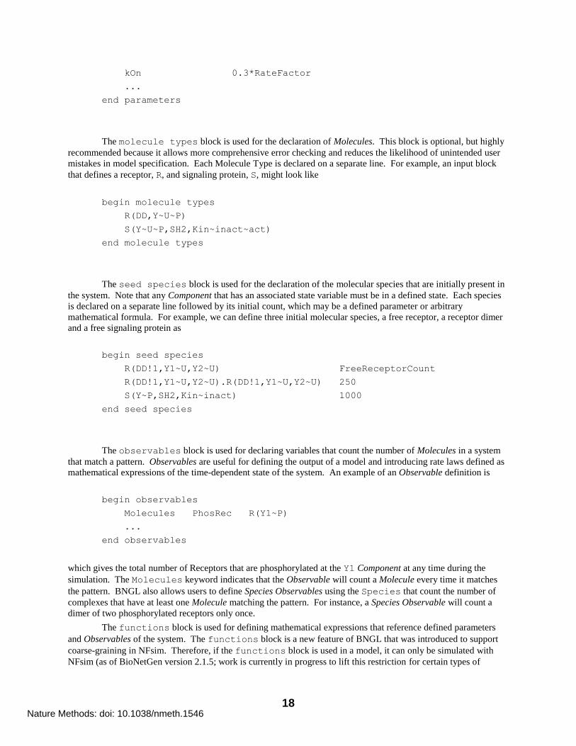
The parameters block is used to declare numerical parameters that designate initial Molecule numbers

and rate constants. Each parameter is declared on a separate line with the parameter name followed by the

parameter value. Parameters can be either single numeric values or arbitrary mathematical expressions that

reference other parameters already defined. For example:

begin parameters

FreeReceptorCount 500

RateFactor 10


http://bionetgen.org/

18

kOn 0.3*RateFactor

...

end parameters

The molecule types block is used for the declaration of Molecules. This block is optional, but highly

recommended because it allows more comprehensive error checking and reduces the likelihood of unintended user

mistakes in model specification. Each Molecule Type is declared on a separate line. For example, an input block

that defines a receptor, R, and signaling protein, S, might look like

begin molecule types

R(DD,Y~U~P)

S(Y~U~P,SH2,Kin~inact~act)

end molecule types

The seed species block is used for the declaration of the molecular species that are initially present in

the system. Note that any Component that has an associated state variable must be in a defined state. Each species

is declared on a separate line followed by its initial count, which may be a defined parameter or arbitrary

mathematical formula. For example, we can define three initial molecular species, a free receptor, a receptor dimer

and a free signaling protein as

begin seed species

R(DD!1,Y1~U,Y2~U) FreeReceptorCount

R(DD!1,Y1~U,Y2~U).R(DD!1,Y1~U,Y2~U) 250

S(Y~P,SH2,Kin~inact) 1000

end seed species

The observables block is used for declaring variables that count the number of Molecules in a system

that match a pattern. Observables are useful for defining the output of a model and introducing rate laws defined as

mathematical expressions of the time-dependent state of the system. An example of an Observable definition is

begin observables

Molecules PhosRec R(Y1~P)

...

end observables

which gives the total number of Receptors that are phosphorylated at the Y1 Component at any time during the

simulation. The Molecules keyword indicates that the Observable will count a Molecule every time it matches

the pattern. BNGL also allows users to define Species Observables using the Species that count the number of

complexes that have at least one Molecule matching the pattern. For instance, a Species Observable will count a

dimer of two phosphorylated receptors only once.

The functions block is used for defining mathematical expressions that reference defined parameters

and Observables of the system. The functions block is a new feature of BNGL that was introduced to support

coarse-graining in NFsim. Therefore, if the functions block is used in a model, it can only be simulated with

NFsim (as of BioNetGen version 2.1.5; work is currently in progress to lift this restriction for certain types of


19

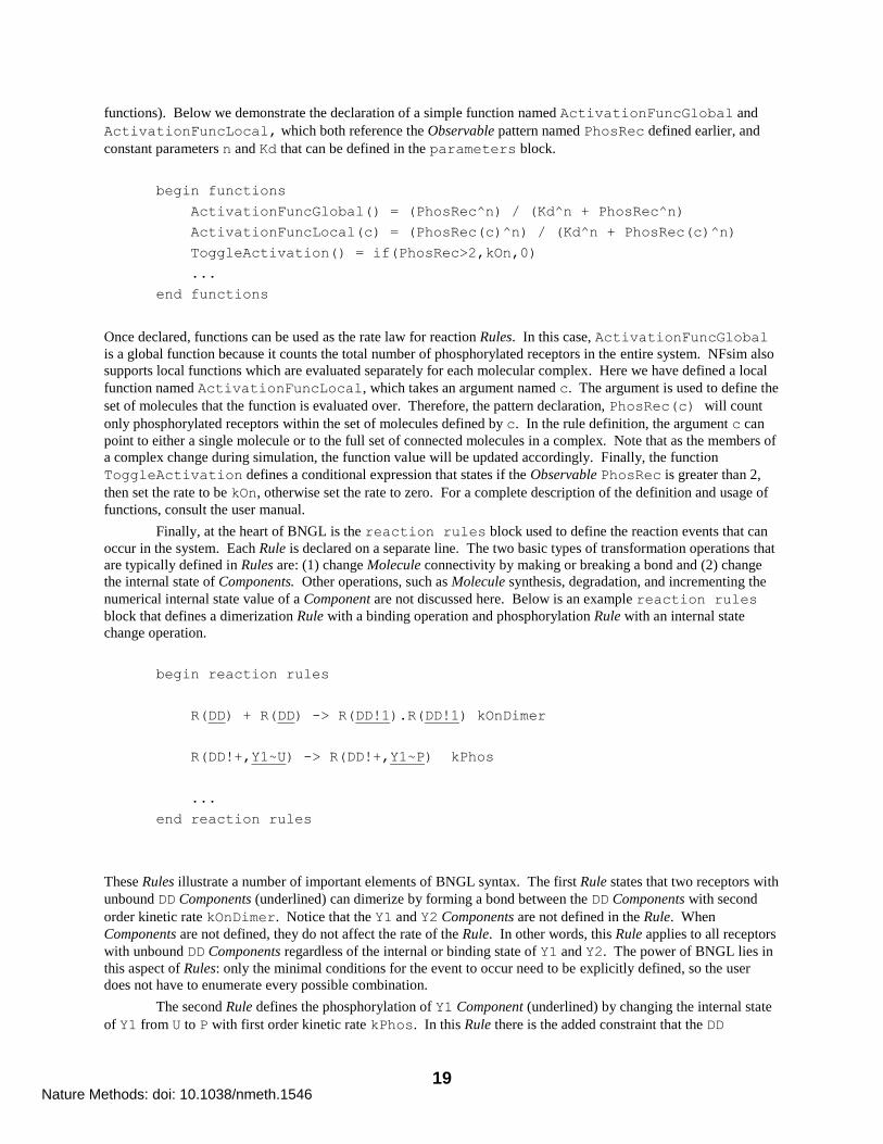
functions). Below we demonstrate the declaration of a simple function named ActivationFuncGlobal and

ActivationFuncLocal, which both reference the Observable pattern named PhosRec defined earlier, and

constant parameters n and Kd that can be defined in the parameters block.

begin functions

ActivationFuncGlobal() = (PhosRec^n) / (Kd^n + PhosRec^n)

ActivationFuncLocal(c) = (PhosRec(c)^n) / (Kd^n + PhosRec(c)^n)

ToggleActivation() = if(PhosRec>2,kOn,0)

...

end functions

Once declared, functions can be used as the rate law for reaction Rules. In this case, ActivationFuncGlobal

is a global function because it counts the total number of phosphorylated receptors in the entire system. NFsim also

supports local functions which are evaluated separately for each molecular complex. Here we have defined a local

function named ActivationFuncLocal, which takes an argument named c. The argument is used to define the

set of molecules that the function is evaluated over. Therefore, the pattern declaration, PhosRec(c) will count

only phosphorylated receptors within the set of molecules defined by c. In the rule definition, the argument c can

point to either a single molecule or to the full set of connected molecules in a complex. Note that as the members of

a complex change during simulation, the function value will be updated accordingly. Finally, the function

ToggleActivation defines a conditional expression that states if the Observable PhosRec is greater than 2,

then set the rate to be kOn, otherwise set the rate to zero. For a complete description of the definition and usage of

functions, consult the user manual.

Finally, at the heart of BNGL is the reaction rules block used to define the reaction events that can

occur in the system. Each Rule is declared on a separate line. The two basic types of transformation operations that

are typically defined in Rules are: (1) change Molecule connectivity by making or breaking a bond and (2) change

the internal state of Components. Other operations, such as Molecule synthesis, degradation, and incrementing the

numerical internal state value of a Component are not discussed here. Below is an example reaction rules

block that defines a dimerization Rule with a binding operation and phosphorylation Rule with an internal state

change operation.

begin reaction rules

R(DD) + R(DD) -> R(DD!1).R(DD!1) kOnDimer

R(DD!+,Y1~U) -> R(DD!+,Y1~P) kPhos

...

end reaction rules

These Rules illustrate a number of important elements of BNGL syntax. The first Rule states that two receptors with

unbound DD Components (underlined) can dimerize by forming a bond between the DD Components with second

order kinetic rate kOnDimer. Notice that the Y1 and Y2 Components are not defined in the Rule. When

Components are not defined, they do not affect the rate of the Rule. In other words, this Rule applies to all receptors

with unbound DD Components regardless of the internal or binding state of Y1 and Y2. The power of BNGL lies in

this aspect of Rules: only the minimal conditions for the event to occur need to be explicitly defined, so the user

does not have to enumerate every possible combination.

The second Rule defines the phosphorylation of Y1 Component (underlined) by changing the internal state

of Y1 from U to P with first order kinetic rate kPhos. In this Rule there is the added constraint that the DD


20

Component must be bound for the reaction to occur indicated by the „!+‟ following the DD Component. Notice

again the omission of the Y2 Component of R, which means that the Rule is applied regardless of the state of the Y2

Component.

In any particular Rule, multiple internal state changes or binding and unbinding operations can be applied

to arbitrarily large molecular complexes. Although the Rules shown here are irreversible, BNGL also permits the

definition of reversible reactions by defining a Rule with the double headed arrow, „<->‟, and providing a second

rate constant or functional rate law.

Compatibility of NFsim models with SBML and CellML. In order for modeling methods such as NFsim to gain

widespread adoption in biological research, standardized modeling protocols and specification formats need to be

developed. Although this is still an active area of research in computational and systems biology, some standards

are beginning to emerge. The most notable projects thus far that aim to standardize the specification of executable

biochemical models include the Systems Biology Markup Language (SBML)55

and CellML56

. These projects help

to facilitate the exchange of models and allow researchers to build on and test existing models. At the time of this

writing, however, NFsim models are not generally compatible with these popular formats because these formats do

not support the definition of reaction rules and the coarse-graining features of NFsim. Instead, both SBML and

CellML formats require a separate entry for each molecular species and possible reaction.

With that in mind, BioNetGen and NFsim does provide the option to convert a rule-based BNGL or NFsim

model into an equivalent SBML format in certain cases. This conversion is only possible when the full reaction

network can be generated from the rule-set and will not work if any of NFsim‟s coarse-graining features are utilized

by the model. This conversion also necessarily loses information regarding the rules and the types of molecules in

the system, so it cannot replace the BNGL format for specifying NFsim models.

In developing NFsim, a new XML-based translation of BNGL was developed to facilitate the loading of

models into NFsim. This new XML format shares some of the key ideas of SBML and may be able to serve as an

early prototype for how rules and coarse-graining features can be added to SBML or other formats. With this XML

infrastructure in place, it will also be straightforward to extend NFsim to support SBML or CellML as soon as they

have the capabilities to encode rules. In fact, there is already a proposed level 3 extension to SBML (L3M at

sbml.org) to do just that. NFsim will be extended to support these standards once they are finalized and accepted by

the systems biology community.


21

Supplementary Note 3 | Detailed comparison to StochSim / DYNSTOC / RuleMonkey / Kappa

To our knowledge StochSim57

, DYNSTOC46

, RuleMonkey47

, and Kappa58

are the only other rule-based,

generalized, biochemical reaction simulators that, like NFsim, use a particle-based representation of molecules to

perform simulations in the well-mixed reaction limit. Here we compare NFsim with these existing platforms and

find that NFsim has important advantages both in capabilities and performance.

StochSim was developed first and presented an algorithm that operates by taking small fixed time steps,

sampling from the set of possible molecules, determining if the two selected molecules react and appropriately

updating the system if a reaction took place. Although the method produces stochastic trajectories of models that

could not be handled easily with ODE or SSA methods, the accuracy of a trajectory may be compromised if too

large a time step is chosen. The method also runs slowly in most situations because during most simulation steps,

no reaction event occurs.

Utilizing a similar algorithm for event propagation, DYNSTOC recently extended the capabilities of

StochSim in two primary ways. First, StochSim is unable to simulate molecular aggregates. Molecular agents in

StochSim can indeed have a large number of binary states, useful for representing posttranslational modification

sites. However, binding events in StochSim produce a new type of molecule, so that molecular connectivity cannot

be tracked in large complexes. DYNSTOC solved this problem by explicitly tracking bonds and binding sites.

Second, DYNSTOC built capabilities to specify models using a formal rule-based language, namely, the BioNetGen

Language54

. Using a formal description of rules greatly simplifies the construction of models and provides a

standard definition for how rules should be interpreted. RuleMonkey, built on the DYNSTOC codebase, and Kappa

utilize a different core algorithm based on Stochastic Simulation Algorithm59

, similar to the algorithm generalized

for NFsim40

. However, unlike NFsim and Yang, et al. RuleMonkey60

uses different method of distinguishing

between intra- and inter- molecular reactions.

Despite these similarities, NFsim has a variety of features that make it much more flexible, efficient and

accessible than other rule-based simulation platforms. First, performance of NFsim for a variety of rule-based

models is superior to Kappa, RuleMonkey and DYNSTOC (Supplementary Table 1). We did not perform direct

runtime comparisons with StochSim because models in StochSim are tedious to specify and cannot handle most of

the systems that we model here. Kappa, RuleMonkey and DYNSTOC also cannot simulate most of the systems

presented in the main text, but simplified versions of these models representing a range of modeling challenges were

used. We find that for all models tested, NFsim is faster than Kappa, DYNSTOC and RuleMonkey. For certain

systems that model the dynamics of aggregation, polymerization or large complexes, we find that NFsim is multiple

orders of magnitude faster, likely due to the significant effort placed on optimizing the way NFsim internally

represents molecular complexes and rules, and extensive optimization of the methods for selecting reactants and

transforming them.

A second clear advantage of NFsim is the ability to define functional or conditional rate laws and other

complex rules. StochSim, DYNSTOC and RuleMonkey do not provide the ability to define functional rates or

coarse-grained rules. Therefore, the actin, bacterial chemotaxis, bacterial flagella and genetic oscillatory models

presented in the main text cannot be simulated with these platforms. This is a severe limitation of existing rule-

based modeling platforms as many systems, particularly those where large complexes form, require special

treatment of cooperativity.

Third, NFsim provides comprehensive output options and a scripting language to control parameters during

simulation. These features are essential for extracting results from a simulation and comparing models to

experimental data, but are absent from other rule-based simulators. For instance, NFsim‟s comprehensive output

capabilities were needed to measure the connectivity of actin filaments and the distribution of actin branching events

in the actin assembly model. The output capabilities were also necessary to measure the activity of chemoreceptor

clusters in the chemotaxis model and the distribution of receptor aggregate sizes in the TLBR model. The scripting

language, on the other hand, was necessary for running simulations where a stimulus was added during simulation,

for instance, to measure the response of chemoreceptors to steps in ligand concentration when validating the

chemoreceptor model. With StochSim, DYNSTOC and RuleMonkey, users would have to write custom software to

extract this type of molecular information.

Fourth, NFsim offers a large suite of supportive tools and features that allow greater accessibility to the

software. For instance, NFsim provides a model debugger for investigating reactions by hand as they occur in a

simulation, Matlab-based parameter scanning and estimation routines, and Matlab-based analysis tools that can

parse and analyze NFsim output. These features allow users to compare NFsim models directly to data in most


22

cases with little effort, and provide a framework for easily incorporating NFsim into other Matlab-based parameter

estimation or model analysis methods.

Finally, NFsim operates with the BioNetGen software platform directly, instead of implementing a separate

BNGL parser as in DYNSTOC and RuleMonkey. Therefore, when changes are made or features are added to the

BioNetGen Language, they are easily, if not immediately, available to NFsim. Furthermore, features new to NFsim,

such as functional rate laws, will be similarly incorporated directly into the definition of the BioNetGen Language.

The compatibility with BioNetGen also aids in the model building process, as a user can run standard ODE and SSA

simulations when possible within the same modeling environment. Taken together, these capabilities make NFsim

more versatile and practical than existing rule-based simulators when facing the difficult modeling challenges of

combinatorial complexity and advanced coarse-grained representations.


23

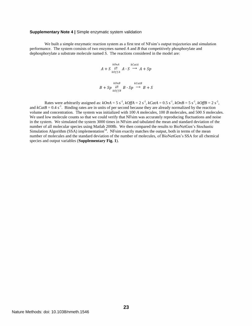
Supplementary Note 4 | Simple enzymatic system validation

We built a simple enzymatic reaction system as a first test of NFsim‟s output trajectories and simulation

performance. The system consists of two enzymes named A and B that competitively phosphorylate and

dephosphorylate a substrate molecule named S. The reactions considered in the model are:

𝐴 + 𝑆

𝑘𝑂𝑛𝐴

⇄ 𝑘𝑂𝑓𝑓𝐴

𝐴 ∙ 𝑆

𝑘𝐶𝑎𝑡𝐴⟶

𝐴 + 𝑆𝑝

𝐵 + 𝑆𝑝

𝑘𝑂𝑛𝐵

⇄ 𝑘𝑂𝑓𝑓𝐵

𝐵 ∙ 𝑆𝑝

𝑘𝐶𝑎𝑡𝐵⟶

𝐵 + 𝑆

Rates were arbitrarily assigned as: kOnA = 5 s-1

, kOffA = 2 s-1

, kCatA = 0.5 s-1

, kOnB = 5 s-1

, kOffB = 2 s-1

,

and kCatB = 0.4 s-1

. Binding rates are in units of per second because they are already normalized by the reaction

volume and concentration. The system was initialized with 100 A molecules, 100 B molecules, and 500 S molecules.

We used low molecule counts so that we could verify that NFsim was accurately reproducing fluctuations and noise

in the system. We simulated the system 3000 times in NFsim and tabulated the mean and standard deviation of the

number of all molecular species using Matlab 2008b. We then compared the results to BioNetGen‟s Stochastic

Simulation Algorithm (SSA) implementation54

. NFsim exactly matches the output, both in terms of the mean

number of molecules and the standard deviation of the number of molecules, of BioNetGen‟s SSA for all chemical

species and output variables (Supplementary Fig. 1).


24

Supplementary Note 5 | Trivalent-ligand, bivalent-receptor (TLBR) validation and performance

As a more thorough validation test and measure of simulation performance, we simulated the trivalent-

ligand, bivalent-receptor (TLBR) system which has served as a model framework for studying receptor aggregation

and signaling in the immune system41

. The TLBR model consists of cell surface receptors that can be crosslinked to

form large aggregates through the intermediate binding of trivalent ligand molecules (Supplementary Fig. 2).

Although there are only three classes of reactions in the system, free ligand binding, receptor-ligand unbinding, and

receptor crosslinking, the resulting number of possible molecular species and reactions is practically infinite. The

TLBR system provides a good test case because it exhibits a high degree of combinatorial complexity but also has a

known analytic solution for its equilibrium behavior61

.

The „effective‟ reaction network size of the TLBR system can be tuned by adjusting the crosslinking

parameter k

XR

tot/ k

off, where Xk is the crosslinking rate,

k

offis the receptor-ligand unbinding rate, and

R

totis the

total number of receptors. As increases, the size of receptor aggregates also increases. Above the critical value

of 4 , a gel phase emerges in which a large fraction of the receptors coalesce into a single giant aggregate41

.

We validated the output trajectory of NFsim against a problem specific stochastic simulator of the TLBR

system and compared distributions of receptor aggregate sizes to the analytic steady-state solution40, 41

. The kinetics

obtained from NFsim and an exact problem-specific simulator40

for two different parameter sets match exactly

(Supplementary Fig. 3a). Furthermore, the distributions predicted by the steady-state analytic solution41

also

precisely match the results produced by NFsim for two different parameter sets (Supplementary Fig. 3b).

The ability to tune the effective network size in the TLBR system provides a way to measure the

performance scaling of NFsim. In the original TLBR model, receptor aggregates are prohibited from forming closed

loop cycles or rings. The non-local connectivity checks needed to prevent rings can be handled in NFsim, but

produce a linear increase in runtime with respect to the number of receptors when simulations are performed under

conditions that produce a gel phase40

. This is reflected in the simulation cost per event of NFsim for 4 when

rings are prohibited (Supplementary Fig. 6a – blue circles). If we do not check for rings and allow any reaction

event to occur, the performance of NFsim is independent of the size of the reaction network (Supplementary Fig.

6a – red squares).

Standard ODE and stochastic methods cannot handle the TLBR system because of the enormous number of

chemical species and reactions that would have to be enumerated. However, we can compare NFsim‟s performance

to an “on-the-fly” SSA simulation run with BioNetGen (Supplementary Fig. 4a – black circles). The “on-the-fly”

SSA operates by incrementally extending the reaction network as needed during the course of a simulation 62, 63

.

The method allows the TLBR system to be simulated relatively efficiently as long as the cross-linking parameter is

low enough ( 0.1 ) such that large aggregates do not form (with ~103 possible molecular species). As we increase

the reaction network size (to 0.2 , with ~105 possible molecular species), however, the reaction network quickly

becomes too large to handle and the “on-the-fly” simulation crashes to a halt. Note that for 0.5 , it becomes

nearly impossible to calculate the full number of possible molecular species and reactions.

NFsim‟s algorithm is agent-based, so it is also helpful to measure how performance scales with the number

of molecules in the system. When checks for cycles are omitted, we find that even when large aggregates form

( 90 ), NFsim‟s performance is nearly independent of the number of molecules in the system (Supplementary

Fig. 6b). The only practical constraint on the size of simulations is on memory, which scales linearly with the total

number of molecule agents for a fixed rule-set (Supplementary Fig. 6b). Although this memory requirement limits

the total number of molecules that can be explicitly tracked in NFsim to a few million, the coarse-graining features

of the platform allow modelers to easily incorporate simple molecules such as ATP without explicit representation

or additional memory cost.


25

Supplementary Note 6 | TLBR parameter scanning and estimation

We used the TLBR model presented in Supplementary Note 5 to demonstrate the parameter scanning and

estimation tools that come packaged with NFsim. In general, data fitting and parameter estimation of stochastic

models is an open problem and the subject of intense and active research64

. Nonetheless, it is useful to have a

software infrastructure that enables users to construct and test different parameter estimation methods and conduct

parameter scanning of models. NFsim includes a set of Matlab-based scripts that provide a framework for

parameter scanning and estimation methods, which are documented in the user manual of NFsim.

The TLBR model was originally conceived to study receptor-ligand binding and the early signaling events

in mast cells of the immune system41

. Recently, flow cytometry experiments of fluorescently labeled trivalent

ligand measured the steady-state fraction of receptor sites that are bound to the FcεRI receptors of mast cells 65

. In

the original study, a problem-specific simulator was implemented to model the TLBR system and custom fitting

code was used to constrain the free parameters of the TLBR model based on the new experimental data. Therefore,

we used the parameter estimation approach followed by this study as a demonstration and validation of NFsim‟s

parameter scanning and estimation feature.

In the original study65

, the concentration of trivalent ligand was varied over six orders of magnitude to

measure the equilibrium binding curve of receptors to ligand. To compare simulations to this type of data, it is

necessary to run simulations over the full range of ligand concentrations and then calculate the steady-state fraction

of receptor sites bound to ligand for each case. We did so using the parameter scanning tool included with NFsim,

as shown in the main text, in Figure 3d. Steady-state values for varying ligand concentrations are computed by

allowing the system to reach steady-state, then averaging over 1000 simulation seconds. Note that in order to

compare the measurements of flow cytometry experiments directly to the fraction of bound receptor sites in

simulations, it is necessary to introduce a non-dimensional scaling term, α, to rescale the experimental

measurements. To be consistent with the original study, we set α=0.816.

Next, we fit the TLBR model to the experimental data as an example of how NFsim can be used to estimate

unknown model parameters. In the TLBR model, there are two free parameters, K1 and K2, which are binding

constants that control initial binding of free ligand to a cell surface receptor and the subsequent crosslinking of two

receptors through mutual ligand binding. To constrain the parameters, we utilized Matlab‟s nonlinear, least-squares

fitting routine. The binding constants obtained with the NFsim fit are within the range of values estimated in the

original study65

. A more complete analysis would include confidence intervals for the parameter estimates, which

could be generated by extending the scripts to implement a bootstrap resampling procedure as was performed in the

original study.

Cross-linked and aggregated receptors in mast cells activate downstream signaling and histamine release

from granules (degranulation), which induce inflammation. Recent experiments measured the fraction of cells that

are degranulated as a function of ligand concentration45

, providing an independent validation of the TLBR model

and the fitted parameters. We compared the TLBR model with the fitted parameters to the degranulation data as

was performed previously65

. The fraction of receptors that are cross-linked in simulations can be used as a simple

measure of cellular degranulation response, and is consistent with the rescaled degranulation data (Supplementary

Fig. 7).


26

Supplementary Note 7 | Multisite phosphorylation model

Similar to the push-pull enzymatic system (Supplementary Note 4), the multisite phosphorylation model

consists of a substrate protein, S, that can be phosphorylated and dephosphorylated by a kinase, K, and phosphatase,

D, respectively. However here, the substrate protein has n independent phosphorylation sites. Each phosphorylation

site can be phosphorylated or not and can be bound or unbound to a kinase or phosphatase. Thus, for each

phosphorylation site, there are 4 distinct states of phosphorylation and binding (phosphorylated and unbound,

unphosphorylated and unbound, phosphorylated and bound to a phosphatase, unphosphorylated and bound to a

kinase). The number of distinct chemical species including the free kinase and phosphatase molecules is 4n+2, as

shown in Figure 1b. For every phosphorylation site, there are 6 distinct rules. The substrate can participate in each

of the 6 rules independently of the state of the remaining n-1 sites. Therefore, when fully expanded, each rule

represents 4n-1

distinct reactions. There are 6n rules, so the number of total reactions in the system is 6·n·(4n-1

),

which is the value plotted in Figure 1b.

The binding, unbinding, and catalytic parameters were chosen to be the same for each phosphorylation site,

although in general they can be varied independently. The rates were assigned as: kOnA = 0.7 s-1

, kOffA = 3 s-1

,

kCatA = 5 s-1

, kOnB = 0.7 s-1

, kOffB = 3 s-1

, and kCatB = 5.1 s-1

, where kOnA and kOffA are binding and unbinding

rates of the kinase to a phosphorylated substrate site, kOnB and kOffB are binding and unbinding of the phosphatase

to an unphosphorylated substrate site, and kCatA and kCatB are the catalytic rates of the kinase and phosphatase

respectively. For simulations, we used 300 kinases, 300 phosphatases, and 3000 substrate proteins.

The average value and noise levels of the output trajectories of the multisite phosphorylation model

simulated with NFsim match exactly the output of validated SSA simulations for cases that could be simulated with

the SSA, providing additional validation of the software (data not shown).


27

Supplementary Note 8 | Compendium of early FcRI signaling models

We also tested NFsim on a series of models of early biochemical events triggered by the stimulation of the

immune-recognition receptor FcRI. For each of the models described below, we compared the simulation output of

in NFsim to equivalent simulations using BioNetGen‟s SSA and find the results match exactly (data not shown).

The base model of FcRI signaling, listed as the model named „JI‟ in Supplementary Table 2, was described in

Supplementary Ref. 66

and includes 354 species and 3680 reactions specified by 24 rules (counting each bi-

directional rule as two separate rules). Four molecule types are included in the base model: a bivalent ligand that

binds receptor from two equivalent sites, a receptor that has a single ligand-binding site and a pair of

phosphorylation sites β and γ, a Src-family protein tyrosine kinase called Lyn that can bind the β site of the receptor

with low affinity when the β site is unphosphorylated and high affinity when the β site is phosphorylated, and the

Syk protein tyrosine kinase that binds the phosphorylated form of the receptor γ site and has two sites of tyrosine

phosphorylation. Receptor-associated Lyn can transphosphorylate the adjacent receptor in a dimer on both

phosphorylation sites, which provides mechanisms to recruit Syk to the complex as well as Lyn through its high-

affinity interaction. Both Lyn and Syk may transphosphorylate Syk that is bound to the same receptor dimer, albeit

on distinct sites. Activation of Syk by phosphorylation of its activation loop site occurs through

transphosphorylation by another Syk molecule and represents the output of the base model. Simulations of the base

model led to a number of predictions relating to the cellular copy numbers of the involved proteins and highlighted

the importance of kinetic proofreading of ligand-receptor interactions for signal transmission (reviewed in

Supplementary Ref. 67

).

Here, we have used the model as the basis for studying how model size may increase as new components

and their interactions are added and how the increased network size may affect performance of simulations that rely

on network generation. In the „JI Red‟ model, the base model was simplified by removing the linker

phosphorylation site Syk (NL), which has no effect on the dynamics of the remaining sites and so can be considered

an „exact‟ reduced model. To expand the base model, the following elements were introduced: a phosphorylation

site on Lyn that is phosphorylated in receptor dimers by Lyn in trans (LP), another Src-family kinase member, Fyn,

was introduced that binds the phosphorylated receptor β site and is phosphorylated in receptor dimers by Lyn in

trans (FYN), a second state of the bivalent ligand was added to increase combinatorial complexity (LIG), a

degenerate γ site was added to the receptor to more accurately model the dimeric γ2 subunit of FcRI (G2), the

number of receptor binding sites on the ligand was increased from two to three (TRI). The incorporation of each of

these modifications (named in parenthesis) is reflected in the rightmost column of Supplementary Table 1. For each

modification the additional rules that were introduced used the rate constants of the most closely related rules

present in the base model, so that no new numerical parameters were introduced.


28

Supplementary Note 9 | Actin assembly, branching and severing models

We built a model of actin filament assembly, branching and severing in order to find a steady-state regime

where branched actin structures can be dynamically maintained through a balance between polymerization /

branching reactions with depolymerization / severing reactions. The system is difficult to model with standard

simulation methods because the actin filaments can exist in an enormous number of states. Each actin subunit in a

filament is either in the ATP bound state, the ADP-Pi bound state, or the ADP bound state. Additionally, subunits

can bind the ADF/cofilin severing complex and the Arp2/3 branching complex. Each subunit can therefore exist in

minimally 5 distinct states, giving rise to 5n states per filament of size n subunits. Filament structures commonly

reach lengths of a thousand subunits or more, making traditional simulation impossible.

To build the rule-based model in NFsim, we focused primarily on the work of two previous efforts. The

first study by Roland and coworkers built a problem-specific simulator to study the dynamic assembly and severing

of actin filaments in the absence of branching reactions42

. The second study by Beltzner and coworkers focused on

modeling the Arp2/3 and VCA mediated nucleation of new branches, but without explicit consideration of the

severing of filaments or the lengths of filaments50

.

First, we reproduced the results of the Roland et al study for an actin filament without branching. The

model uses the same assumptions as the original study for cofilin mediated severing, actin subunit hydrolysis, and

actin subunit phosphate release. The model only follows one actin filament at a time and assumes a fixed bulk

concentration of actin monomers and ADF/cofilin molecules in solution. To maintain a constant pool of monomers,

we used NFsim‟s ability to define conditional functions. Whenever a segment of the filament was discarded, it is

removed from the simulation. If an actin monomer or ADF/cofilin complex binds a filament, a conditional rule is

immediately activated to produce another available monomer or ADF/cofilin complex. Although there are other

ways to add this type of constraint to an NFsim model, such as creating new actin subunits immediately during the

polymerization reaction, we found that conditional rules were the most straightforward. Our rule-based version of

the Roland et al model matches the results originally described (Supplementary Fig. 4). The NFsim result is both

an added validation of our software and a confirmation that we have correctly interpreted the Roland et al model.

The Beltzner et al study, on the other hand, focused on the nucleation of new branches off of existing

filaments. Combining ODE modeling with experiments, they show that the molecular mechanism of nucleating new

branches likely arises from a particular sequence of interactions and activation events between VCA, Arp2/3

complex, an actin monomer, and an actin filament. Namely, they propose that the primary mechanism of nucleating

new branches involves first binding of VCA to a free actin monomer; second, VCA-actin binding to an Arp2/3

complex; third, the entire complex binding an actin filament; fourth, a first order activation of the structure; and

finally, the elongation of the new branch. We adopted these same assumptions and reaction steps in our model.

Absent from both models, but important in the dynamics of actin assembly, is the action of the capping

protein. Capping protein binds strongly to barbed ends of filaments to halt continued elongation. Capping protein

both constrains the length of filaments that can form and will influence the steady-state size of branched actin

structures that form. Therefore, we added capping reactions to the combined model based on mechanisms

documented in the literature51, 53, 68

. Our final model of actin assembly, together with the rule-based version of the

Roland et al model, is provided on the NFsim website.

To provide further validation of the actin model and demonstrate how the Matlab-based tools of NFsim can

be used to compare models directly to experiments, we compared the actin model predictions to the results of a

highly cited study that monitored actin branching in real-time69

. In these experiments, a fraction of actin monomers

were fluorescently labeled and all monomers were allowed to polymerize in a flow cell. Arp2/3 complex and

branching cofactors were passed through the flow cell allowing branches to form off existing filaments. Branching

and polymerization could then be visualized using total internal reflection fluorescence (TIRF) microscopy. These

experiments were used to measure the distribution of branch points from the barbed ends of both existing filaments

and portions of filaments that polymerized after addition of Arp2/3.

To compare the actin model directly to these experiments, it is necessary to recreate the multiple steps of

the experiment and extract information from simulations about the connectivity of filaments and branches. We

accomplished this by using NFsim‟s simple scripting language, which allows model parameters to change at specific

time points during simulation, together with NFsim‟s comprehensive output functionality. We also wrote Matlab

scripts to automate the process of running simulations and visualizing results. In comparing the actin model to this

dataset, it was also necessary to reduce the rate of actin polymerization to reflect the reduced activity of

fluorescently labeled actin as was measured in the original study. We also had to introduce a nucleation reaction to


29

allow the formation of new filaments at the beginning of the experiment. The NFsim run script that specifies the

multiple experimental steps of the NFsim simulation and the modified model that includes reduced polymerization

and the nucleation reaction are available online. The actin model is indeed consistent with the experimental results

as presented in Figure 4b and Figure 4c of the main text.

Although our simulations of the actin model are not spatially resolved, it is useful to generate 3D

renderings of the branched structures to visualize their topology and the connectivity of the filaments

(Supplementary Videos 1 and 2). We generated the 3D renderings with Matlab 2008b assuming that there is a 13

subunit helical twist in actin filaments and that branches form at 70 degree angles off of those filaments oriented in a

direction that is based on the period of the twist at the branch point. In the 3D renderings, the diameter of the

filaments and the twist is enlarged so they can be better visualized.

In the main text, we used the actin model to achieve a dynamic steady-state regime where branching and

polymerization reactions are compensated by severing and depolymerization reactions. We then made predictions

about the length and distribution of filaments and branches in connected actin structures. The parameters used in

those simulations are drawn directly from experimental measurements or are reasonable estimates that have been

used in past modeling efforts. However, the concentrations of proteins involved in the actin assembly system are

highly variable across different organisms, cell types and even across a single cell. Therefore, we tuned those

parameters within reason based on published measurements. An explanation of how we chose the concentration

parameters is provided here.

There is high variability in the concentration of actin monomers across species and conditions ranging from

2 to 100M49

. The concentration of monomers that are available is likely much lower, however, because free actin

in cells can be sequestered by molecules such as thymosin-4, a protein found in vertebrates. For models described

here, we take the concentration of available actin monomers to be 8M, which is on the same order of magnitude as

estimates of previously described models42, 50

.

Measurements of total ADF/cofilin in cells range from 3 to 30M, a high proportion of which will be

bound to actin filaments49

. We take the concentration of available ADF/cofilin to be 2M, similar to the value used

in past modeling efforts42

.

Measurements of total Arp2/3 complex range from 2 to 10M, of which some will be bound to polymer

branch points or pointed ends49

. We take the concentration of available Arp2/3 to be 5M. The VCA domain of

WASp/Scar proteins binds Arp2/3 to promote nucleation and branching activity of Arp2/3. The concentration of

available VCA will vary as the cell responds to stimuli. We find that a concentration of 0.5M, the value used in an

existing model50

, is sufficient to produce a sustained steady-state filament growth in the presence of capping protein.

The concentration of total capping protein in the cell has been measured at approximately 1M49, 51

. Given

the strength of the interaction between capping protein and free barbed ends of polymers, Kim et. al. estimate that

90% of the cell‟s capping protein will be bound to barbed ends, consistent with our simulation results51

. Thus we

assume that there is 0.1M of capping protein available to bind free barbed ends.

Concentration parameters used for this study are summarized in Supplementary Table 3. Rate constant

parameters, organized by biochemical process, are provided in Supplementary Tables 4 to 7.


30

Supplementary Note 10 | Model of bacterial chemoreceptor adaptation

We built a new model of bacterial chemotaxis response and adaptation based on the Assistance

Neighborhood (AN) model43, 44

. As discussed in the main text, bacteria sense external chemicals through highly

cooperative signaling teams of chemoreceptors70

. Individual receptors are methylated and demethylated at four

distinct sites by CheR and CheB enzymes. In addition to binding the active sites directly, CheR and CheB can bind

a second site, typically called the tether or tethering site, on a short flexible domain at the C-terminus of receptors.

The tethering site is needed to accelerate the otherwise slow kinetics of methylation and demethylation.

Additionally, once CheR or CheB is bound to the tethering site, it can modify neighboring receptors‟ active sites.

The neighborhood of receptors that a tethered enzyme can modify is what gives the AN model its name.

Simulating the details of receptor activity and adaptation is challenging. First, just like the multisite

phosphorylation model, the complexity of multiple methylation sites per receptor presents combinatorial difficulties

in model specification and simulation. Second, the topology of chemoreceptors needed to handle the tethering

reactions of CheR and CheB cannot be represented with standard ODE or SSA simulation methods. Finally, the

cooperativity of chemoreceptor signaling teams requires calculation of a free energy term during simulation for each

signaling team individually, which cannot be handled by any existing generalized simulator.

NFsim meets all of these requirements to allow the first general specification of the AN model. In the

original formulation, a tightly packed array of 19 receptor dimers on a hexagonal lattice was represented with an

allosteric Monod-Wyman-Changeux (MWC) model whereby the entire signaling team switches cooperatively and

rapidly between active (on) and inactive (off) states. The probability to be in the active state is defined as a function

of the external concentration of ligand and the individual methylation state of receptor dimers and is parameterized

by m , the free energy contribution of a receptor dimer methylated at m sites, Kon(r,l), the binding constant of receptor

of type r for ligand of type l if the cluster is in the on state, and Koff(r,l), the binding constant of receptor of type r for

ligand of type l in the off state. Although there are multiple types of receptors, only the most abundant types, TAR

and TSR, were modeled. The free energy function and derivation can be found in Supplementary Ref. 44

. For all of

our simulations, we use the same parameter values as the original study, namely, 0=1.0, 1=0.5, 2=0.0, 3=-0.3,

4=-0.6, 5=-0.85, 6=-1.1, 7=-2.0, 8=-3.0, Kon(TAR,asp)=0.5 mM, Koff(TAR,asp)=0.02 mM, Kon(TSR,asp)=106 mM, and

Koff(TSR,asp)= 100 mM, where asp represents the chemoattractant aspartate.

In the original model, individual CheR and CheB molecules are not tracked, but are both assumed to have a

first order binding rate to the tether of 0.01 s-1

and an unbinding rate of 0.1 s-1

. Once bound to a tether, the model

assumes saturated enzyme kinetics throughout the receptor neighborhood with CheR methylation at a rate of 0.1 s-1

and CheB demethylation at a rate 0.2 s-1

. In NFsim, we model multiple signaling teams simultaneously and

explicitly represent CheR and CheB molecules. Our simulations consider ~14,000 receptors, in line with

experimental measurements of cells grown in rich media71

. We then choose CheR/CheB numbers to be 500 each in

order to match the occupancy of tethers and timescale of adaptation assumed in the original model. We choose a

reasonably fast binding rate (2.8 M-1

s-1

) to the tether for both CheR and CheB while keeping the same unbinding

and catalytic rates as the original model. Our implementation of the rule-based model can accurately reproduce the

original results and captures the dynamics of adaptation well (Supplementary Fig. 5).

Building on our general rule-based version of the AN model, we updated the connectivity of receptor

dimers to reflect new cryo-electron microscopy results72, 73

. In the original model, neighborhoods could maximally

consist of up to seven receptor dimers (a central dimer connected to six others) due to the assumed tight hexagonal

packing. The cryo-electron experiments show that receptor packing is not as tight, with receptors arranged in

trimers of dimers. In the new configuration, the length of the flexible tether would limit neighborhoods to only four

dimers, the three immediately connected in a trimer and the next closest dimer in a neighboring trimer. In this

configuration for a cluster of 18 dimers, there are six neighborhoods of three dimers and twelve neighborhoods of

four dimers. Simulations of the full model, as explained in the main text, can account for the wide dynamic range

and sensitivity of bacterial chemical sensing. Furthermore, simulations of the full chemoreceptor adaptation model

are efficient, taking just ~3 minutes on a desktop machine to produce the trajectories of an entire cell as shown in

Figure 5c of the main text.


31

Supplementary Note 11 | Coarse-grained model of the bacterial flagellar motor

We built a coarse-grained model of the bacterial flagellar motor to demonstrate how global functions can

be used to model complex reaction dynamics or simplify chemical processes when mechanistic details are not well

known. The flagellar motor switches between clockwise (CW) and counter-clockwise (CCW) rotation to control the

characteristic run and tumble motion of chemotactic bacteria70

. Binding of the phosphorylated form of the diffusible

signaling protein CheY to the base of the motor influences the probability to be in the CW or CCW state74

. A

complete picture of the physical steps involved in switching rotational states is still missing, but as discussed in the

main text, a coarse-grained two-state model can capture the dynamic behavior well and is useful for studying signal

processing in single cells75, 76

.

In the two-state model, states correspond to either CW or CCW rotation. The free energy barrier, G ,

between states as a function of CheY-P concentration, assuming binding of CheY-P to the motor is much faster than

the timescale of motor switching, can be written as

0 1 [ ]

4 2 [ ]

g g YpG

Yp Kd

,

where 1 [ ]

2 [ ]

g Yp

Yp Kd

characterizes the free energy contribution of CheY-P binding the motor with binding constant

Kd , cellular CheY-P concentration [ ]Yp , and the free parameters 0g and 1g which are in units Bk T . Then, the rate

of switching between rotational states can be written as

/ BG k Tk e

,

where k is the rate of transition from CW to CCW, k is the rate of transition from CCW to CW, and is a

parameter that controls the rate of switching. For our models in NFsim, we created a molecule that coarse-grains the

motor with CW or CCW rotational states. The rate of switching states depends functionally on the number of

phosphorylated CheY molecules. The CheY molecules and its phosphorylation and dephosphorylation reactions can

be connected to any upstream signaling cascade, but for simplicity we keep the concentration constant for any single

simulation. A constant phosphorylated CheY concentration is a reasonable approximation for fitting the model

parameters to single-cell experiments where the motor response curve was measured74

. Next we used global

functions to encode the mathematical expressions of the free energy barrier and switching rates. In our simulations,

we choose the parameters as 3.06Kd M , 0 1 35 Bg g k T , and 11.02 s to fit experimental measurements of

motor dynamics in unstimulated single cells74

.


32

Supplementary Note 12 | Negative feedback oscillator model

We constructed a model of oscillating gene expression to demonstrate how high-level approximations, such

as treating gene regulation as an on/off switch, can be easily incorporated into dynamic models with NFsim.

Simulations of the model also illustrate how different coarse-grained representations and assumptions are

interchangeable in NFsim and can lead to very different model behaviors77

. Oscillations in the model are driven by

a negative feedback loop with an explicit time delay that arises from protein synthesis and nuclear shuttling. The

model is derived from Supplementary Ref 78

, and consists of the following reactions:

∅

𝑘∙𝑓([𝑃𝑟𝑜𝑡𝑁𝑢𝑐 ])

⟶

𝑚𝑅𝑁𝐴𝑁𝑢𝑐

𝑚𝑅𝑁𝐴𝑁𝑢𝑐

𝑘𝐸𝑥𝑝𝑜𝑟𝑡⟶

𝑚𝑅𝑁𝐴𝐶𝑦𝑡 𝑃𝑟𝑜𝑡𝐶𝑦𝑡

𝑘𝐼𝑚𝑝𝑜𝑟𝑡

⟶

𝑃𝑟𝑜𝑡𝑁𝑢𝑐

𝑚𝑅𝑁𝐴𝐶𝑦𝑡

𝑘𝑇𝑟𝑎𝑛𝑠⟶

𝑚𝑅𝑁𝐴𝐶𝑦𝑡 + 𝑃𝑟𝑜𝑡𝐶𝑦𝑡

𝑚𝑅𝑁𝐴𝐶𝑦𝑡

𝑘𝐷𝑒𝑔 1

⟶

∅ 𝑚𝑅𝑁𝐴𝑁𝑢𝑐

𝑘𝐷𝑒𝑔 2

⟶

∅ 𝑃𝑟𝑜𝑡𝐶𝑦𝑡

𝑘𝐷𝑒𝑔 3

⟶

∅ 𝑃𝑟𝑜𝑡𝑁𝑢𝑐

𝑘𝐷𝑒𝑔 4∙[𝑃𝑟𝑜𝑡 𝑁𝑢𝑐 ]

𝐾𝑚𝐷𝑒𝑔 + [𝑃𝑟𝑜𝑡 𝑁𝑢𝑐 ]

⟶

∅

where 𝑓([𝑃𝑟𝑜𝑡𝑁𝑢𝑐 ]) is the repression rate as a function of the nuclear localized protein. This function is chosen to

be either a Boolean on/off switch, a piecewise linear function, or a Hill function, which can all be represented as

functional or conditional expressions in NFsim. These functions are defined as:

𝐵𝑜𝑜𝑙𝑒𝑎𝑛 𝑃𝑟𝑜𝑡𝑁𝑢𝑐 = 𝑘𝑚𝑎𝑥

0

𝑖𝑓 𝑃𝑟𝑜𝑡𝑁𝑢𝑐 ≤ 𝐾𝐷

𝑜𝑡𝑕𝑒𝑟𝑤𝑖𝑠𝑒

𝐿𝑖𝑛𝑒𝑎𝑟 𝑃𝑟𝑜𝑡𝑁𝑢𝑐 = 𝑘𝑚𝑎𝑥

0𝑘𝑚𝑎𝑥 ∙ (𝑥0 𝑃𝑟𝑜𝑡𝑁𝑢𝑐 + 𝑥1)

𝑖𝑓 𝑃𝑟𝑜𝑡𝑁𝑢𝑐 ≤ 𝑏0

𝑖𝑓 𝑃𝑟𝑜𝑡𝑁𝑢𝑐 ≥ 𝑏1

𝑜𝑡𝑕𝑒𝑟𝑤𝑖𝑠𝑒

𝐻𝑖𝑙𝑙 𝑃𝑟𝑜𝑡𝑁𝑢𝑐 =𝑘𝑚𝑎𝑥 ∙ 𝐾𝐷

𝑛

𝐾𝐷𝑛 + 𝑃𝑟𝑜𝑡𝑁𝑢𝑐

𝑛

We set the parameters of the repression functions so that each produces 50% repression of transcription at 25 copies

of nuclear localized protein with 𝐾𝐷=25. For the Hill function, the Hill coefficient 𝑛 was set to 4. Parameters of the

Linear function were selected to match the steepest part of the Hill function curve, with 𝑥0=-0.0391 and 𝑥1=1.4775.

To ensure that the Linear function only evaluates to values between 𝑘𝑚𝑎𝑥 and 0, we set the bounds of the Linear

function to be 𝑏0=12 and 𝑏1=38 copies of nuclear protein. The remaining parameters were chosen to produce

sustained oscillations as determined in Supplementary Ref 78

by setting 𝑘=10000 min-1

, 𝑘𝑚𝑎𝑥 =1 min-1

, 𝑘𝐸𝑥𝑝𝑜𝑟𝑡=0.2

min-1

, 𝑘𝐼𝑚𝑝𝑜𝑟𝑡=0.1 min-1

, 𝑘𝑇𝑟𝑎𝑛𝑠=0.1 min-1

, 𝑘𝐷𝑒𝑔1=0.2 min-1

, 𝑘𝐷𝑒𝑔2=10min-1

, 𝑘𝐷𝑒𝑔3=0.1 min-1

, 𝑘𝐷𝑒𝑔4=8

min-1

, and 𝐾𝑚𝐷𝑒𝑔=10. Initial concentrations of all molecules were set to zero.

In Figure 6 of the main text, the periods of oscillation are 37.4, 34.6 and 33.3 minutes for the

Boolean, linear and Hill functions respectively, while the magnitudes of the mRNA peaks are 1480188,

1120214 and 790253 molecules. The period of oscillation was calculated by identifying the peak of the

power spectrum of the molecule number traces. The magnitudes and standard deviations of the mRNA peaks were

calculated by computing a 10 minute sliding average to smooth the trajectories and identifying the peak of each gene

expression cycle.


33

Supplementary References

40. Yang, J., Monine, M.I., Faeder, J.R. & Hlavacek, W.S. Kinetic Monte Carlo method for rule-based

modeling of biochemical networks. Phys. Rev. E 78, 031910 (2008).

41. Goldstein, B. & Perelson, A.S. Equilibrium theory for the clustering of bivalent cell surface receptors by

trivalent ligands. Application to histamine release from basophils. Biophys. J. 45, 1109-1123 (1984).

42. Roland, J., Berro, J., Michelot, A., Blanchoin, L. & Martiel, J.L. Stochastic Severing of Actin Filaments by

Actin Depolymerizing Factor/Cofilin Controls the Emergence of a Steady Dynamical Regime. Biophys. J.

94, 2082-2094 (2008).

43. Hansen, C.H., Endres, R.G. & Wingreen, N.S. Chemotaxis in Escherichia coli: a molecular model for

robust precise adaptation. PLoS Comput. Biol. 4, e1 (2008).

44. Endres, R.G. & Wingreen, N.S. Precise adaptation in bacterial chemotaxis through "assistance

neighborhoods". Proc. Natl. Acad. Sci. USA 103, 13040-13044 (2006).

45. Posner, R.G. et al. Trivalent antigens for degranulation of mast cells. Organic Letters 9, 3551-3554 (2007).

46. Colvin, J. et al. Simulation of large-scale rule-based models. Bioinformatics 25, 910-917 (2009).

47. Colvin, J. et al. RuleMonkey: software for stochastic simulation of rule-based models. BMC Bioinformatics

11, 404 (2010).

48. Danos, V., Feret, J., Fontana, W., Harmer, R. & Krivine, J. Rule-Based Modelling of Cellular Signalling.

Lect. Notes. Comput. Sci. 4703, 17-41 (2007).

49. Pollard, T.D., Blanchoin, L. & Mullins, R.D. Molecular Mechanisms Controlling Actin Filament Dynamics

in Nonmuscle Cells. Annu. Rev. Biophys. Biomol. Struct. 29, 545-576 (2000).

50. Beltzner, C.C. & Pollard, T.D. Pathway of Actin Filament Branch Formation by Arp2/3 Complex. J. Biol.

Chem. 283, 7135-7144 (2008).

51. Kim, K., Yamashita, A., Wear, M.A., Maeda, Y. & Cooper, J.A. Capping protein binding to actin in yeast:

biochemical mechanism and physiological relevance. J. Cell Biol. 164, 567-580 (2004).

52. Pollard, T.D. Rate constants for the reactions of ATP- and ADP-actin with the ends of actin filaments. J.

Cell Biol. 103, 2747-2754 (1986).

53. Schafer, D.A., Jennings, P.B. & Cooper, J.A. Dynamics of capping protein and actin assembly in vitro:

uncapping barbed ends by polyphosphoinositides. J. Cell Biol. 135, 169-179 (1996).

54. Faeder, J.R., Blinov, M.L. & Hlavacek, W.S. Rule-Based Modeling of Biochemical Systems with

BioNetGen. Methods Mol. Biol. 500, 113-167 (2009).

55. Hucka, M. et al. The systems biology markup language (SBML): a medium for representation and

exchange of biochemical network models. Bioinformatics 19, 524-531 (2003).

56. Miller, A. et al. An overview of the CellML API and its implementation. BMC Bioinformatics 11, 178-178

(2010).

57. Le Novere, N. & Shimizu, T.S. STOCHSIM: modelling of stochastic biomolecular processes.

Bioinformatics 17, 575-576 (2001).

58. Danos, V., Feret, J., Fontana, W. & Krivine, J. Scalable Simulation of Cellular Signaling Networks. Lect.

Notes. Comput. Sci. 4807, 139-157 (2007).

59. Gillespie, D.T. A general method for numerically simulating the stochastic time evolution of coupled

chemical reactions. J. Comput. Phys. 22, 403-434 (1976).

60. Yang, J. & Hlavacek, W.S. Rejection-free kinetic Monte Carlo simulation of multivalent biomolecular

interactions. Arxiv preprint arXiv:0812.4619 (http://arxiv.org/abs/0812.4619) (2010).

61. Goldstein, B. & Perelson, A.S. Equilibrium theory for the clustering of bivalent cell surface receptors by

trivalent ligands. Application to histamine release from basophils. Biophys J 45, 1109-1123 (1984).

62. Faeder, J.R., Blinov, M.L., Goldstein, B. & Hlavacek, W.S. Rule-based modeling of biochemical networks.

Complexity 10, 22-41 (2005).

63. Lok, L. & Brent, R. Automatic generation of cellular reaction networks with Moleculizer 1.0. Nat.

Biotechnol. 23, 131-136 (2005).

64. Poovathingal, S.K. & Gunawan, R. Global parameter estimation methods for stochastic biochemical

systems. BMC Bioinformatics 11, 414 (2010).

65. Monine, M.I., Posner, R.G., Savage, P.B., Faeder, J.R. & Hlavacek, W.S. Modeling multivalent ligand-

receptor interactions with steric constraints on configurations of cell-surface receptor aggregates. Biophys.

J. 98, 48-56 (2010).


http://arxiv.org/abs/0812.4619

34

66. Faeder, J.R. et al. Investigation of Early Events in FcRI-Mediated Signaling Using a Detailed

Mathematical Model. J. Immunol. 170, 3769-3781 (2003).

67. Goldstein, B., Faeder, J.R. & Hlavacek, W.S. Mathematical and computational models of immune-receptor

signalling. Nature Reviews. Immunology 4, 445-456 (2004).

68. Pollard, T.D. & Borisy, G.G. Cellular Motility Driven by Assembly and Disassembly of Actin Filaments.

Cell 112, 453-465 (2003).

69. Amann, K.J. & Pollard, T.D. Direct real-time observation of actin filament branching mediated by Arp2/3

complex using total internal reflection fluorescence microscopy. Proc. Natl. Acad. Sci. USA 98, 15009-

15013 (2001).

70. Wadhams, G.H. & Armitage, J.P. Making sense of it all: bacterial chemotaxis. Nat. Rev. Mol. Cell Biol. 5,

1024-1037 (2004).

71. Li, M. & Hazelbauer, G.L. Cellular Stoichiometry of the Components of the Chemotaxis Signaling

Complex. J. Bacteriol. 186, 3687-3694 (2004).

72. Briegel, A. et al. Location and architecture of the Caulobacter crescentus chemoreceptor array. Mol.

Microbiol. 69, 30-41 (2008).

73. Khursigara, C.M., Wu, X. & Subramaniam, S. Chemoreceptors in Caulobacter crescentus: Trimers of

Receptor Dimers in a Partially Ordered Hexagonally Packed Array. J. Bacteriol. 190, 6805-6810 (2008).

74. Cluzel, P., Surette, M. & Leibler, S. An Ultrasensitive Bacterial Motor Revealed by Monitoring Signaling

Proteins in Single Cells. Science 287, 1652-1655 (2000).

75. Fall, C., Marland, E., Wagner, J. & Tyson, J. Computational Cell Biology. (Springer, 2005).

76. Tu, Y. & Grinstein, G. How White Noise Generates Power-Law Switching in Bacterial Flagellar Motors.

Phys. Rev. Lett. 94, 208101-208104 (2005).

77. Mather, W., Bennett, M.R., Hasty, J. & Tsimring, L.S. Delay-Induced Degrade-and-Fire Oscillations in

Small Genetic Circuits. Phys. Rev. Lett. 102, 068105-068105 (2009).

78. Novak, B. & Tyson, J.J. Design principles of biochemical oscillators. Nat Rev Mol Cell Biol 9, 981-991

(2008).


efficient modeling, simulation and coarse-graining of ... modeling, simulation and coarse-graining...

Documents