cmsc 421 spring 2004 section 0202 contents...

1

CMSC 421 Spring 2004 Section 0202

Part II: Process ManagementChapter 6

CPU Scheduling

Silberschatz, Galvin and Gagne 20026.2Operating System Concepts

Contents

Basic ConceptsScheduling Criteria Scheduling AlgorithmsMultiple-Processor SchedulingReal-Time SchedulingAlgorithm Evaluation


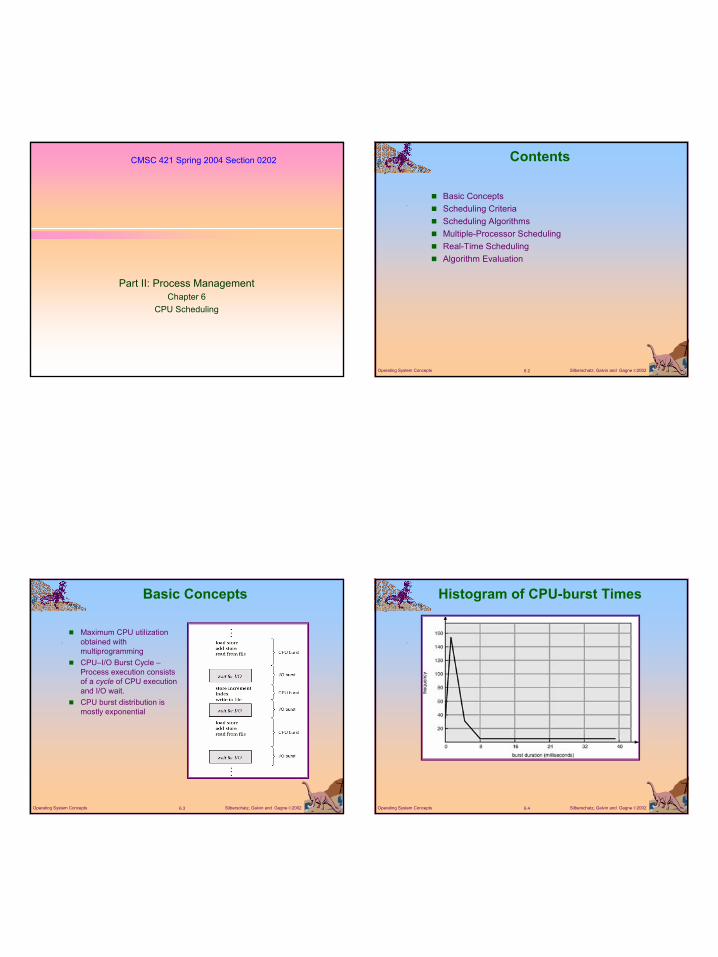
Basic Concepts

Maximum CPU utilization obtained with multiprogrammingCPU–I/O Burst Cycle –Process execution consists of a cycle of CPU execution and I/O wait.CPU burst distribution is mostly exponential


Histogram of CPU-burst Times

2


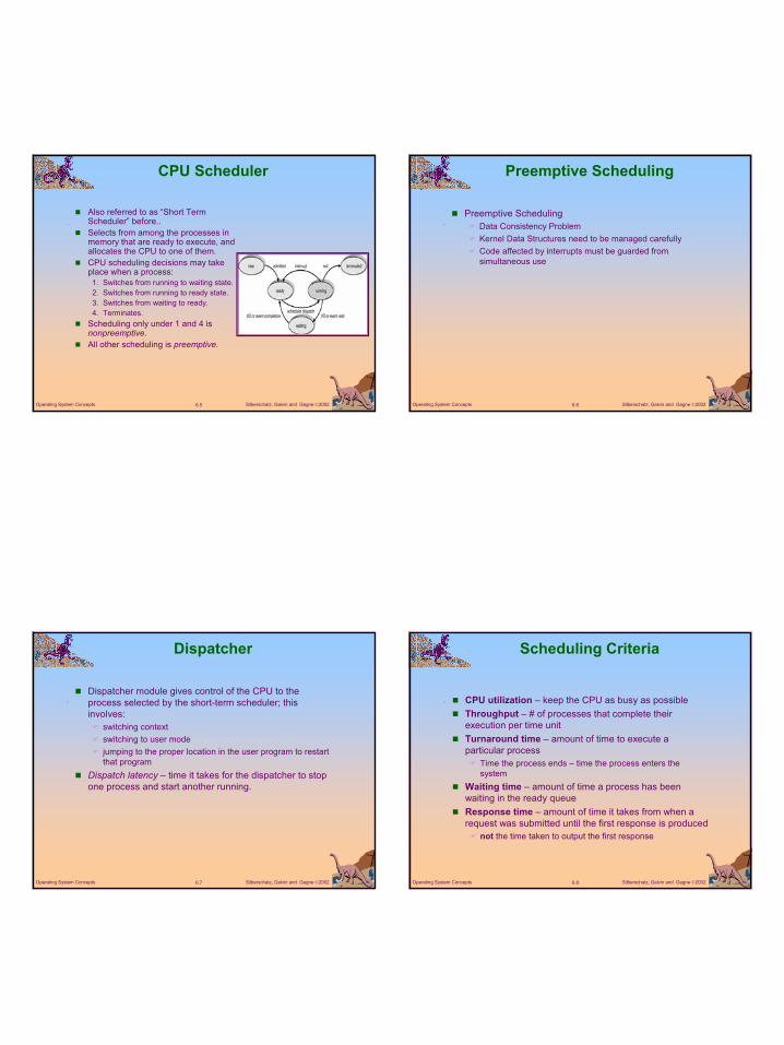
CPU Scheduler

Also referred to as “Short Term Scheduler” before..Selects from among the processes in memory that are ready to execute, and allocates the CPU to one of them.CPU scheduling decisions may take place when a process:

1. Switches from running to waiting state.2. Switches from running to ready state.3. Switches from waiting to ready.4. Terminates.

Scheduling only under 1 and 4 is nonpreemptive.All other scheduling is preemptive.


Preemptive Scheduling

Preemptive SchedulingData Consistency ProblemKernel Data Structures need to be managed carefullyCode affected by interrupts must be guarded from simultaneous use


Dispatcher

Dispatcher module gives control of the CPU to the process selected by the short-term scheduler; this involves:

switching contextswitching to user modejumping to the proper location in the user program to restart that program

Dispatch latency – time it takes for the dispatcher to stop one process and start another running.


Scheduling Criteria

CPU utilization – keep the CPU as busy as possibleThroughput – # of processes that complete their execution per time unitTurnaround time – amount of time to execute a particular process

Time the process ends – time the process enters the system

Waiting time – amount of time a process has been waiting in the ready queueResponse time – amount of time it takes from when a request was submitted until the first response is produced

not the time taken to output the first response

3


Optimization Criteria

Max CPU utilizationMax throughputMin turnaround time Min waiting time Min response timeOther optimizations

Minimize variance in response timeMinimize the maximum response time

Each process typically consists of 100 of CPU/IO burstsWe consider 1 CPU burst/process in the description of the algorithms


First-Come, First-Served (FCFS) Scheduling

Process Burst TimeP1 24P2 3P3 3

Suppose that the processes arrive in the order: P1 , P2 , P3 The Gantt Chart for the schedule is:

Waiting time for P1 = 0; P2 = 24; P3 = 27Average waiting time: (0 + 24 + 27)/3 = 17

P1 P2 P3

24 27 300


FCFS Scheduling (Cont.)

Suppose that the processes arrive in the orderP2 , P3 , P1 .

The Gantt chart for the schedule is:

Waiting time for P1 = 6; P2 = 0; P3 = 3Average waiting time: (6 + 0 + 3)/3 = 3Much better than previous case

P1P3P2

63 300


FCFS (Cont.)

Convoy EffectShorter processes (with smaller CPU bursts) waiting behind a longer CPU-bound process

FCFS in non-preemptiveCPU is held by the currently executing process UNTIL

An I/O request comesProcess terminates

4


Shortest-Job-First (SJF) Scheduling

Associate with each process the length of its next CPU burst. Use these lengths to schedule the process with the shortest CPU burst.Two schemes:

nonpreemptive – once CPU given to the process it cannot be preempted until completes its CPU burst.preemptive – if a new process arrives with CPU burst length less than remaining time of current executing process, preempt the executing process. This scheme is know as the Shortest-Remaining-Time-First (SRTF).


SJF (Cont.)

SJF is optimal – gives minimum average waiting time for a given set of processes.SJF could lead to starving processes

Process waits for CPU while other processes with shorter bursts get priority


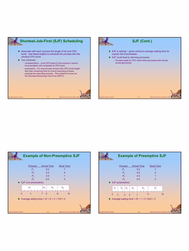
Process Arrival Time Burst TimeP1 0.0 7P2 2.0 4P3 4.0 1P4 5.0 4

SJF (non-preemptive)

Average waiting time = (0 + 6 + 3 + 7)/4 = 4

Example of Non-Preemptive SJF

P1 P3 P2

73 160

P4

8 12


Example of Preemptive SJF

Process Arrival Time Burst TimeP1 0.0 7P2 2.0 4P3 4.0 1P4 5.0 4

SJF (preemptive)

Average waiting time = (9 + 1 + 0 +2)/4 = 3

P1 P3P2

42 110

P4

5 7

P2 P1

16

5


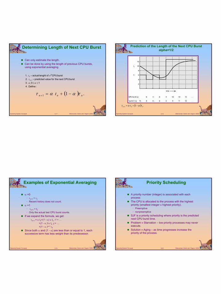
Determining Length of Next CPU Burst

Can only estimate the length.Can be done by using the length of previous CPU bursts, using exponential averaging.

:Define 4.10 , 3.

burst CPU next the for value predicted 2.burst CPU of lenght actual 1.

≤≤=

=

+

αατ 1n

thn nt

( ) .1 1 nnn t ταατ −+=+


Prediction of the Length of the Next CPU Burstalpha=1/2

( ) .1 1 nnn t ταατ −+=+


Examples of Exponential Averaging

α =0τn+1 = τn

Recent history does not count.α =1

τn+1 = tnOnly the actual last CPU burst counts.

If we expand the formula, we get:τn+1 = α tn+(1 - α) α tn -1 + …

+(1 - α )j α tn -j + …+(1 - α )n+1 τ0

Since both α and (1 - α) are less than or equal to 1, each successive term has less weight than its predecessor.


Priority Scheduling

A priority number (integer) is associated with each processThe CPU is allocated to the process with the highest priority (smallest integer ≡ highest priority).

Preemptivenonpreemptive

SJF is a priority scheduling where priority is the predicted next CPU burst time.Problem ≡ Starvation – low priority processes may never execute.Solution ≡ Aging – as time progresses increase the priority of the process.

6


Round Robin (RR)

Each process gets a small unit of CPU time (time quantum or slice), usually 10-100 milliseconds. After this time slice has elapsed, the process is preempted and added to the end of the ready queue.If there are n processes in the ready queue and the time quantum is q, then each process gets 1/n of the CPU time in chunks of at most q time units at once.

No process waits more than (n-1)q time units.When deciding on the time slice need to consider the overhead due to the dispatcherPerformance characteristics

q large ⇒ FIFOq small ⇒ q must be large with respect to context switch, otherwise overhead is too high (processor sharing)


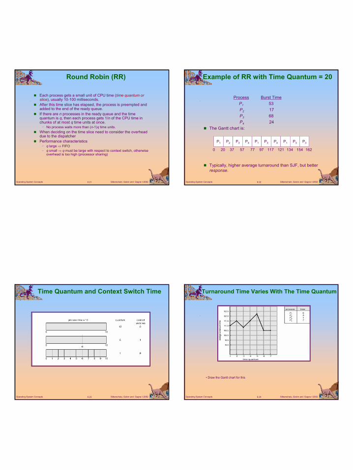
Example of RR with Time Quantum = 20

Process Burst TimeP1 53P2 17P3 68P4 24

The Gantt chart is:

Typically, higher average turnaround than SJF, but better response.

P1 P2 P3 P4 P1 P3 P4 P1 P3 P3

0 20 37 57 77 97 117 121 134 154 162


Time Quantum and Context Switch Time


Turnaround Time Varies With The Time Quantum

• Draw the Gantt chart for this

7


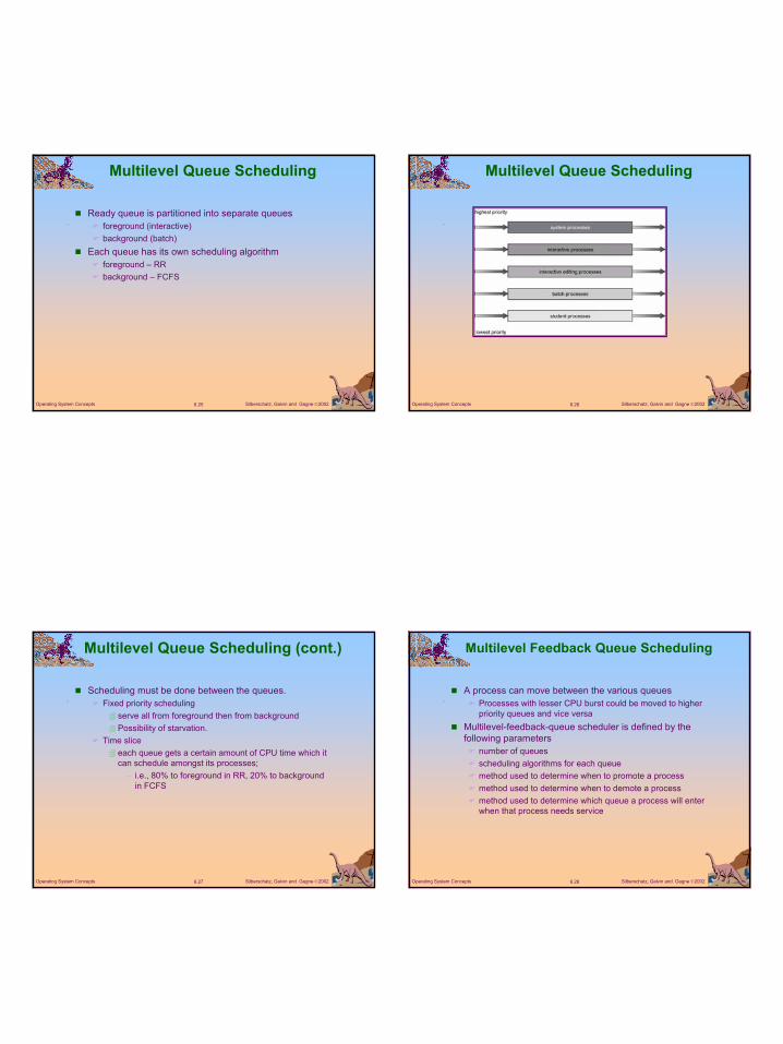
Multilevel Queue Scheduling

Ready queue is partitioned into separate queuesforeground (interactive)background (batch)

Each queue has its own scheduling algorithm foreground – RRbackground – FCFS


Multilevel Queue Scheduling


Multilevel Queue Scheduling (cont.)

Scheduling must be done between the queues.Fixed priority scheduling

serve all from foreground then from backgroundPossibility of starvation.

Time sliceeach queue gets a certain amount of CPU time which it can schedule amongst its processes;

– i.e., 80% to foreground in RR, 20% to background in FCFS


Multilevel Feedback Queue Scheduling

A process can move between the various queuesProcesses with lesser CPU burst could be moved to higher priority queues and vice versa

Multilevel-feedback-queue scheduler is defined by the following parameters

number of queuesscheduling algorithms for each queuemethod used to determine when to promote a processmethod used to determine when to demote a processmethod used to determine which queue a process will enter when that process needs service

8


Multilevel Feedback Queues


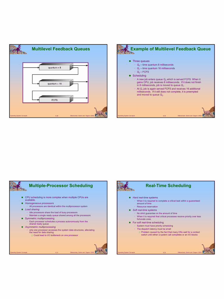
Example of Multilevel Feedback Queue

Three queuesQ0 – time quantum 8 millisecondsQ1 – time quantum 16 millisecondsQ2 – FCFS

SchedulingA new job enters queue Q0 which is served FCFS. When it gains CPU, job receives 8 milliseconds. If it does not finish in 8 milliseconds, job is moved to queue Q1.At Q1 job is again served FCFS and receives 16 additional milliseconds. If it still does not complete, it is preempted and moved to queue Q2.


Multiple-Processor Scheduling

CPU scheduling is more complex when multiple CPUs are available.Homogeneous processors

All processors are identical within the multiprocessor systemLoad sharing

Idle processors share the load of busy processorsMaintain a single ready queue shared among all the processors

Symmetric multiprocessingEach processor schedules a process autonomously from the shared ready queue

Asymmetric multiprocessingonly one processor accesses the system data structures, alleviating the need for data sharing.

Could lead to I/O bottleneck on one processor


Real-Time Scheduling

Hard real-time systems When it is required to complete a critical task within a guaranteed amount of timeResource reservation

Soft real-time systems No strict guarantee on the amount of timeWhen it is required that critical processes receive priority over less fortunate ones.

For soft real-time scheduling System must have priority schedulingThe dispatch latency must be small

Problem caused by the fact that many OSs wait for a context switch until either a system call completes or an I/O blocks

9


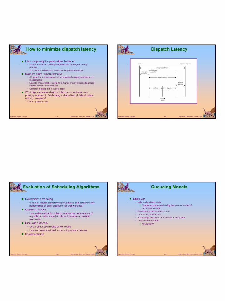
How to minimize dispatch latency

Introduce preemption points within the kernelWhere it is safe to preempt a system call by a higher priority processTrouble is only few such points can be practically added

Make the entire kernel preemptiveAll kernel data structures must be protected using synchronization mechanismsNeed to ensure that it is safe for a higher priority process to access shared kernel data structuresComplex method that is widely used

What happens when a high priority process waits for lower priority processes to finish using a shared kernel data structure (priority inversion)?

Priority inheritance


Dispatch Latency


Evaluation of Scheduling Algorithms

Deterministic modelingtake a particular predetermined workload and determine the performance of each algorithm for that workload

Queueing ModelsUse mathematical formulas to analyze the performance of algorithms under some (simple and possible unrealistic) workloads

Simulation ModelsUse probabilistic models of workloadsUse workloads captured in a running system (traces)

Implementation


Queueing Models

Little’s LawValid under steady state

Number of processes leaving the queue=number of processes arriving

N=number of processes in queueLamda=avg. arrival rateW= average wait time for a process in the queueLittle’s law states that

N=Lamda*W

10


Evaluation of CPU Schedulers by Simulation


Solaris 2 Scheduling


Windows 2000 Priorities

cmsc 421 spring 2004 section 0202 contents...

Documents