Clustering

James Long

November 10, 2015

1 / 33

Clustering References

I Elements of Statistical Learning (Tibshirani, Hastie, Friedman)

I Chapter 14.3I http://statweb.stanford.edu/~tibs/ElemStatLearn/

I Statistics, Data Mining, and Machine Learning inAstronomy (Ivezic, et al)

I Section 6.4

I Modern Statistical Methods for Astronomy (Feigelson, Babu)

I Sections 9.2 – 9.5

2 / 33

What is clustering?

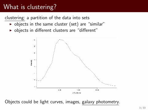
clustering: a partition of the data into setsI objects in the same cluster (set) are “similar”I objects in different clusters are “different”

Objects could be light curves, images, galaxy photometry.3 / 33

Normalized Rest Frame Synthetic Photometry

4 / 33

Notation, Data Dimension, and Clustering

I X ∈ Rn×p

I n is number of observations (galaxies)I p is number of variables / featuresI xi ∈ Rp is i th observation

I p is called the dimension of the data.

I Clustering methods useful for “high” dimensional (p > 3) datawhere we do not have a priori have idea of structure.

5 / 33

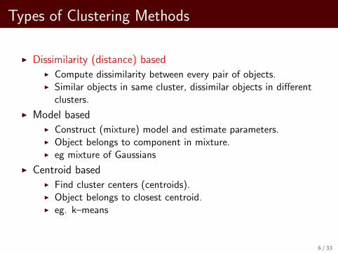
Types of Clustering Methods

I Dissimilarity (distance) basedI Compute dissimilarity between every pair of objects.I Similar objects in same cluster, dissimilar objects in different

clusters.

I Model basedI Construct (mixture) model and estimate parameters.I Object belongs to component in mixture.I eg mixture of Gaussians

I Centroid basedI Find cluster centers (centroids).I Object belongs to closest centroid.I eg. k–means

6 / 33

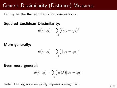
Generic Dissimilarity (Distance) Measures

Let xiλ be the flux at filter λ for observation i .

Squared Euclidean Dissimilarity:

d(xi , xj) =∑λ

(xiλ − xjλ)2

More generally:

d(xi , xj) =∑λ

|xiλ − xjλ|p

Even more general:

d(xi , xj) =∑λ

w(λ)|xiλ − xjλ|p

Note: The log scale implicitly imposes a weight w .7 / 33

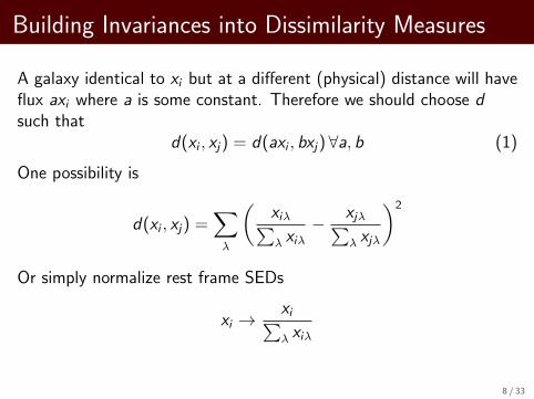
Building Invariances into Dissimilarity Measures

A galaxy identical to xi but at a different (physical) distance will haveflux axi where a is some constant. Therefore we should choose dsuch that

d(xi , xj) = d(axi , bxj)∀a, b (1)

One possibility is

d(xi , xj) =∑λ

(xiλ∑λ xiλ

− xjλ∑λ xjλ

)2

Or simply normalize rest frame SEDs

xi →xi∑λ xiλ

8 / 33

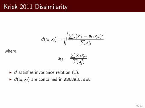
Kriek 2011 Dissimilarity

d(xi , xj) =

√∑λ(xiλ − a12xjλ)2∑

x2iλ

where

a12 =

∑xiλxjλ∑

x2jλ

I d satisfies invariance relation (1).

I d(xi , xj) are contained in AS689 b.dat.

9 / 33

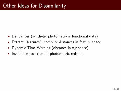
Other Ideas for Dissimilarity

I Derivatives (synthetic photometry is functional data)

I Extract “features”, compute distances in feature space

I Dynamic Time Warping (distance in x,y space)

I Invariances to errors in photometric redshift

10 / 33

Dissimilarity Based Clustering Methods

I Kriek 2011

I Hierarchical agglomerative

I Hierarchical divisive

I See references for other methods.

11 / 33

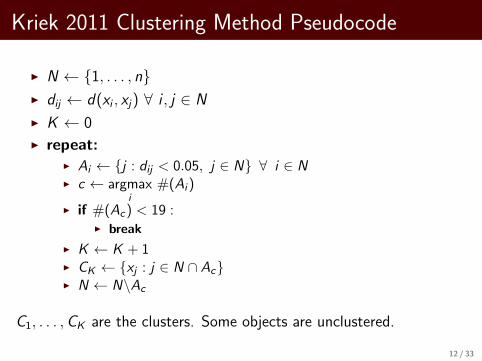
Kriek 2011 Clustering Method Pseudocode

I N ← {1, . . . , n}I dij ← d(xi , xj) ∀ i , j ∈ N

I K ← 0

I repeat:I Ai ← {j : dij < 0.05, j ∈ N} ∀ i ∈ NI c ← argmax

i#(Ai )

I if #(Ac) < 19 :I break

I K ← K + 1I CK ← {xj : j ∈ N ∩ Ac}I N ← N\Ac

C1, . . . ,CK are the clusters. Some objects are unclustered.

12 / 33

Hierarchical Agglomerative Clustering Idea

Main Idea:

I Every observation starts as own cluster.

I Iteratively merge “close” clusters together.

I Iterate until one giant cluster left.

This method is

I Hierarchical: Each iteration produces a clustering, so do notspecify number of clusters in advance.

I Agglomerative: Initially every observation in own cluster.

13 / 33

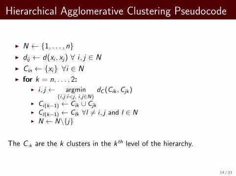
Hierarchical Agglomerative Clustering Pseudocode

I N ← {1, . . . , n}I dij ← d(xi , xj) ∀ i , j ∈ N

I Cin ← {xi} ∀i ∈ N

I for k = n, . . . , 2:I i , j ← argmin

{i ,j :i<j , i ,j∈N}dC (Cik ,Cjk)

I Ci(k−1) ← Cik ∪ Cjk

I Cl(k−1) ← Clk ∀l 6= i , j and l ∈ NI N ← N\{j}

The C·k are the k clusters in the k th level of the hierarchy.

14 / 33

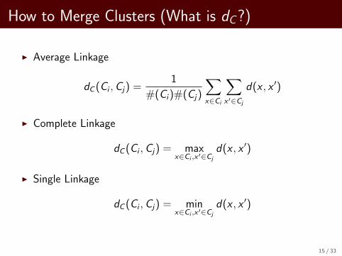
How to Merge Clusters (What is dC?)

I Average Linkage

dC (Ci ,Cj) =1

#(Ci)#(Cj)

∑x∈Ci

∑x ′∈Cj

d(x , x ′)

I Complete Linkage

dC (Ci ,Cj) = maxx∈Ci ,x ′∈Cj

d(x , x ′)

I Single Linkage

dC (Ci ,Cj) = minx∈Ci ,x ′∈Cj

d(x , x ′)

15 / 33

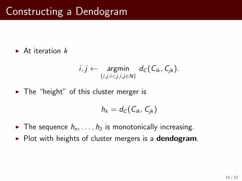
Constructing a Dendogram

I At iteration k

i , j ← argmin{i ,j :i<j ,i ,j∈N}

dC (Cik ,Cjk).

I The “height” of this cluster merger is

hk = dC (Cik ,Cjk)

I The sequence hn, . . . , h2 is monotonically increasing.

I Plot with heights of cluster mergers is a dendogram.

16 / 33

Average Linkage

17 / 33

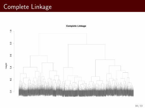
Complete Linkage

18 / 33

Single Linkage

19 / 33

Number of Clusters, Quality of Clustering

I Quantification of success in classification is (relatively) objectiveand easy.

I Quantification of success in clustering is more subjective.I General measures output by clustering method.

I Cophenetic distance.I Confusion matrix to compare clustering methods.

I Application specific measures.I Scatter in composites.I Physical interpretation of clusters.

20 / 33

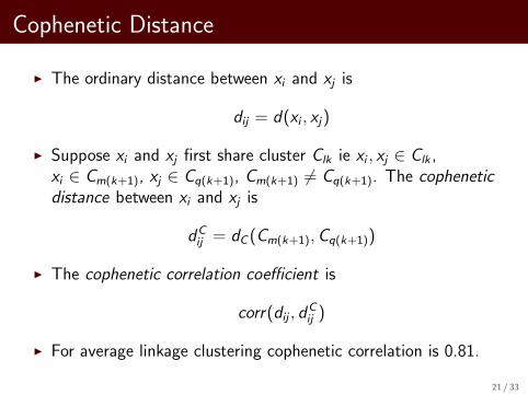
Cophenetic Distance

I The ordinary distance between xi and xj is

dij = d(xi , xj)

I Suppose xi and xj first share cluster Clk ie xi , xj ∈ Clk ,xi ∈ Cm(k+1), xj ∈ Cq(k+1), Cm(k+1) 6= Cq(k+1). The copheneticdistance between xi and xj is

dCij = dC (Cm(k+1),Cq(k+1))

I The cophenetic correlation coefficient is

corr(dij , dCij )

I For average linkage clustering cophenetic correlation is 0.81.

21 / 33

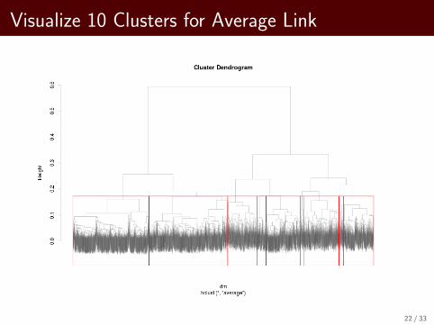
Visualize 10 Clusters for Average Link

22 / 33

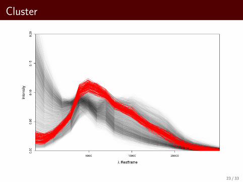
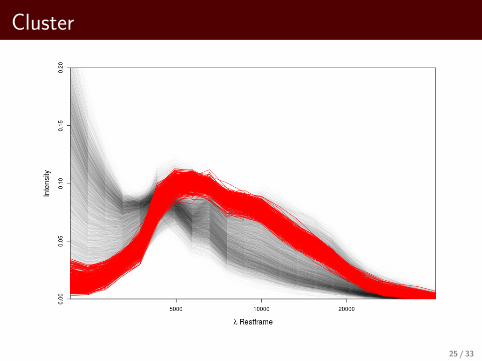
Cluster

23 / 33

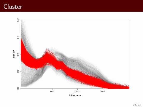
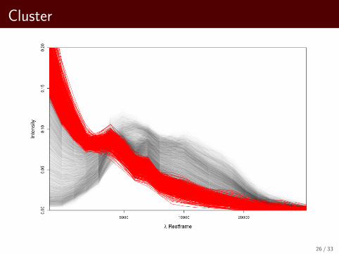
Cluster

24 / 33

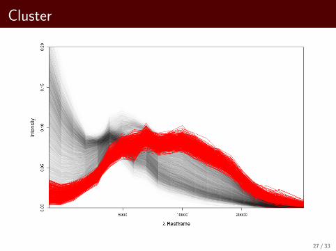
Cluster

25 / 33

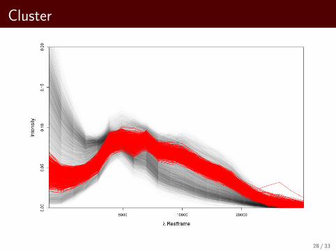
Cluster

26 / 33

Cluster

27 / 33

Cluster

28 / 33

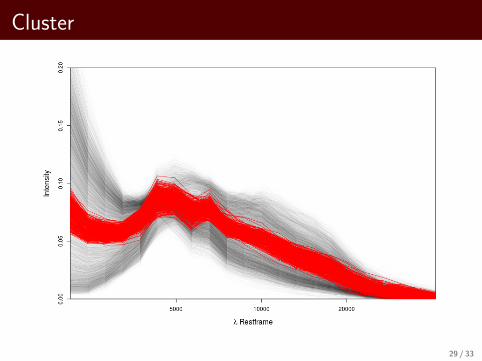
Cluster

29 / 33

Cluster

30 / 33

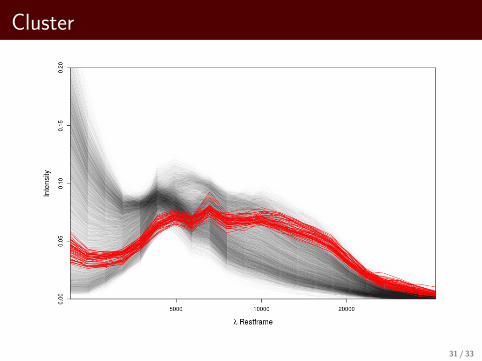
Cluster

31 / 33

Cluster

32 / 33

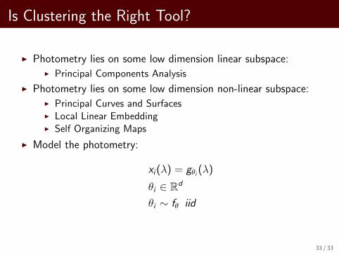
Is Clustering the Right Tool?

I Photometry lies on some low dimension linear subspace:I Principal Components Analysis

I Photometry lies on some low dimension non-linear subspace:I Principal Curves and SurfacesI Local Linear EmbeddingI Self Organizing Maps

I Model the photometry:

xi(λ) = gθi (λ)

θi ∈ Rd

θi ∼ fθ iid

33 / 33