clouds and sulfate are anticorrelated: a new diagnostic

Clouds and sulfate are anticorrelated:

A new diagnostic for global sulfur models

Dorothy KochNASA Goddard Institute for Space Studies, Columbia University, New York, New York, USA

Jeffrey ParkDepartment of Geology and Geophysics, Yale University, New Haven, Connecticut, USA

Anthony Del GenioNASA Goddard Institute for Space Studies, Columbia University, New York, New York, USA

Received 21 March 2003; revised 29 September 2003; accepted 10 October 2003; published 24 December 2003.

[1] We consider the correlation between clouds and sulfate in order to assess the relativeimportance of cloud aqueous-phase production of sulfate, precipatation scavenging ofsulfate, and inhibition of gas-phase sulfate production beneath clouds. Statistical analysisof observed daily cloud cover and sulfate surface concentrations in Europe and NorthAmerica indicates a significant negative correlation between clouds and sulfate. Thisimplies that clouds remove sulfate via precipitation scavenging and/or inhibit sulfate gas-phase production more than they enhance sulfate concentration through aqueous-phaseproduction. Persistent sulfate/cloud anticorrelations at long timescales (8–64 days)apparently result from large-scale dynamical influences on clouds, which in turn impactsulfate. A statistical analysis of output from the general circulation model (GCM) of theGoddard Institute for Space Studies (GISS) shows weak coherence between sulfate andcloud cover. However, there is stronger anticorrelation between the model’s sulfategenerated by gas-phase oxidation and cloud cover. Sulfate/cloud anticorrelation in theGCM strengthens if we extinguish gas-phase sulfate production beneath clouds, as shouldhappen since the oxidant OH is photochemically generated. However the only way toachieve strong anticorrelation between total sulfate and clouds is by correcting ourtreatment of aqueous-phase sulfate production. Our model, like many other global tracermodels, released dissolved species (including sulfate) from clouds after each cloudtime step rather than making release contingent upon cloud evaporation. After correctingthis in the GISS model, more sulfate is rained out, the sulfate burden produced via theaqueous phase decreases to half its former amount, and the total sulfate burden is25% lower. INDEX TERMS: 0305 Atmospheric Composition and Structure: Aerosols and particles

(0345, 4801); 0320 Atmospheric Composition and Structure: Cloud physics and chemistry; 0365 Atmospheric

Composition and Structure: Troposphere—composition and chemistry; 0368 Atmospheric Composition and

Structure: Troposphere—constituent transport and chemistry; KEYWORDS: aerosol

Citation: Koch, D., J. Park, and A. Del Genio, Clouds and sulfate are anticorrelated: A new diagnostic for global sulfur models,

J. Geophys. Res., 108(D24), 4781, doi:10.1029/2003JD003621, 2003.

1. Introduction

[2] The impact of sulfate aerosols on climate may besignificant, but is subject to considerable uncertainty. Themost straightforward impact is the ‘‘direct’’ effect (scatteringof incoming solar radiation back to space). In terms ofanthropogenic radiative forcing the direct effect may be�0.2 to �0.9 W m�2 [Penner et al., 2001]. Potentially moresignificant (but much more uncertain) are the sulfate ‘‘indi-rect’’ effects on cloud radiative properties and lifetime, thefirst and second indirect effects, respectively. The first

indirect effect is estimated to lie between 0 and �2 W m�2

[Penner et al., 2001], but is highly uncertain; and the secondindirect is too uncertain to assign a meaningful forcingrange. Clouds are involved in both the production andremoval of sulfate aerosols. Sulfate is almost entirely derivedfrom oxidation of SO2 either in the gas phase or aqueousphase (i.e., within cloud droplets). Gas-phase productionwill be suppressed beneath clouds due to reduced oxidantOH amounts. Sulfate, being highly soluble, is removedfrom the atmosphere mostly by precipitation scavenging,and to a lesser degree by dry deposition.[3] Cloud processes generate, scavenge and are impacted

by sulfate, but the overall relationship between them is poorly

JOURNAL OF GEOPHYSICAL RESEARCH, VOL. 108, NO. D24, 4781, doi:10.1029/2003JD003621, 2003

Copyright 2003 by the American Geophysical Union.0148-0227/03/2003JD003621$09.00

AAC 10 - 1

known. Do cloudy conditions result in heavy sulfate produc-tion, or do clouds effectively clean the atmosphere of theseaerosols? Do clouds inhibit gas-phase sulfate productionsignificantly? If a single process dominates, we shouldobserve strong correlation between clouds and sulfate, anda diagnostic phase relationship. If in-cloud production dom-inates, sulfate (or its rate-of-change) would be positivelycorrelated with clouds. Negative correlation would resultfrom scavenging and also from gas-phase production sup-pression beneath clouds.[4] Previous studies using global sulfate models indicated

that (model) sulfate generation occurs primarily in clouds.Tables summarizing these studies [see, e.g., Koch et al.,1999; Chin et al., 2000] suggest that most of the sulfate isproduced in the aqueous phase (model estimates range from64% to 89%). Most removal also occurs by wet deposition,typically around 80% (although the budgets are difficult tocompare because some models identify rained-out sulfur assulfate and some as SO2), with the rest removed by drydeposition. Thus it appears that clouds play a highlysignificant role in both the generation and removal of sulfateaerosols. In the work of Koch et al. [1999], our global sulfurmodel indicated a slight tendency toward positive correla-tion between clouds and sulfate near source regions andanticorrelation in more remote regions.[5] Given the level of uncertainty in modeling clouds and

their interactions with the sulfur cycle, it is preferable toobserve correlations in measurements. A number of effortsare now underway to tease out cloud/sulfate relations usingsatellite observations [Schwartz et al., 2002; Lohmann andLesins, 2002]. These studies must confront the problem ofcloud-screening: the determination of where clouds end andaerosol haze begins. A further difficulty is distinguishingbetween sulfate and other aerosol types.[6] Here we use a different approach to observe cloud-

sulfate relations, by making use of the extensive surfaceconcentration data sets that have been saved by Europeanand North American networks. These data provide daily

average concentrations of sulfate. To these we comparecloud satellite products which also have daily resolution. Aswe will show below, there is a strong negative correlationbetween clouds and sulfate. We use these results to test andcorrect our model’s sulfur simulation.

2. Observations of Cloud-Sulfate Correlations

[7] In order to seek correlation between clouds andsulfate, we use daily average sulfate surface concentrationsin Europe from the Cooperative Program for Monitoringand Evaluation of the Long Range Transmission of AirPollutants in Europe (EMEP) [e.g., Schaug et al., 1987] andin North America from the Eulerian Model Evaluation FieldStudy (EMEFS) [e.g., McNaughton and Vet, 1996]. We use4 years of data from EMEP (1989–1992) and 1 year of datafrom EMEFS (1989–1990). We choose sites that have atleast 20 days of sulfate data/month: 21 sites from EMEPand 31 sites from EMEFS. These locations are shown inFigure 1. We also made use of precipitation and sulfatedeposition (i.e., in rainwater) data from the 15 of the EMEPsites that had this information (stars in Figure 1).[8] Total cloud cover comes from the International

Satellite Cloud Climatology Project (ISCCP, version D1)[e.g., Stubenrauch et al., 1999; Rossow and Schiffer, 1999].The satellite observations provide cloud parameters every3 hours which we average to make 24-hour means. Wechose to work with total cloud cover (results using cloudoptical thickness were similar). We gathered time serieswith daily resolution of sulfate surface concentration andtotal cloud cover above the ground-based site.[9] General features of the data series can be discerned

from 4months’ data from one of the EMEP sites (Deuselbach

Figure 1. Map showing locations of sulfate surfaceconcentration and ISCCP cloud cover observations (whitecircles); EMEP sites having precipitation and depositioninformation are marked with stars. Grid boxes used for themodel calculations are triangles (Scandinavia), diamonds(Europe) and inverted triangles (North America).

Figure 2. Time series of cloud cover (%), sulfatesurface concentration (mg S/m3) and sulfate deposition flux(mg S/m2/d) at Deuselbach, Germany (49.8�N 7�E) for thelast 125 days of 1991.

AAC 10 - 2 KOCH ET AL.: CLOUD-SULFATE CORRELATIONS

Germany, 49.8�N 7�E), shown in Figure 2. Here we see thatdecreases in cloud cover typically correlate with increases insulfate surface concentration. Such cloud ‘‘dips’’ can persistfor extensive periods, such as from days 320–350. Peaks indeposition flux generally cluster together in time periods withlow sulfate air concentrations. It is not uncommon for suchclusters to persist for 10–20 days. Thuswe see that the sulfateconcentration rises during relatively clear periods (whenclouds do not inhibit gas-phase production) and decreasesduring cloudy, rainy periods (when precipitating cloudsscavenge sulfate and/or clouds inhibit gas-phase sulfateproduction). In the next section we apply statisticalapproaches to quantify such relationships in the data series.

3. Statistical Methods

[10] For estimating the correlation between cloud coverand sulfate concentration, deposition or precipitation, weapply time series algorithms that use Slepian wavelets [Lillyand Park, 1995; Bear and Pavlis, 1999; Park and Mann,2000]. We use wavelets instead of standard Fourier trans-forms to account for possible nonstationary behavior in the

data correlations. For instance, if aqueous sulfate-produc-tion and cloud-scavenging dominate in different time inter-vals, a wavelet-based correlation estimate can detectcompeting episodes of strong correlation that are sometimespositive, and sometimes negative. Correlation estimatesbased on the Fourier-transform tend to average behaviorover entire time series, and can appear weak if the correla-tion phase varies with time.[11] Slepian wavelets are designed as the counterparts of

Slepian tapers, which are used in multiple taper spectrumanalysis [Thomson, 1982; Park et al., 1987a, 1987b;Percival and Walden, 1993]. In particular, Slepian waveletsare derived from an optimization condition that, for aspectrum estimate at frequency fo, minimizes spectral leak-age outside a specified frequency interval [ fo � fw , fo + fw].The leakage-resistance condition takes the form of aneigenvector problem. Its solution is a sequence of waveletsthat (1) possess optimal spectral leakage properties (2) haveeither odd or even parity, and (3) are mutually orthogonal.Even and odd wavelets can be paired as real and imaginaryparts of a complex-valued wavelet, in order to constrain thephase of a signal. Mutual orthogonality affords statistical

Figure 3. Squared coherence C2 between observed sulfate and cloud cover over Europe summed overeach season for 1989–1992. On the log-period axis, 3, 4, 5, and 6 correspond to oscillation periods of 8,16, 32 and 64 days, respectively. We superimpose a cumulative coherence plot on the gray-scale images.The bars indicate our ‘‘detection level’’ for stacked coherence, estimated to be at least the 98%confidence level for nonrandomness.

KOCH ET AL.: CLOUD-SULFATE CORRELATIONS AAC 10 - 3

independence among wavelet transforms computed withdifferent wavelet pairs.[12] We compute the phased wavelet transform of time

series of observations or GCM model output (describedbelow) at a collection of cycle periods Tk = 1/fk, where fk area set of logarithmically spaced frequencies. We use three

complex-valued Slepian tapers with time-bandwidth p = 2.5[Lilly and Park, 1995] and compute coherence C betweentime series at matching points in time and frequency. Thephase f of the coherence C translates into the time delay orsense of correlation: f � 0� is positive correlation, f �±180� is negative correlation. Note that the phase angle

Figure 4. Same as Figure 3 but for Scandinavia. On the log-period axis, 3, 4, 5, and 6 correspond tooscillation periods of 8, 16, 32 and 64 days, respectively.

Figure 5. Same as Figure 3 but for North American stations, shown for 1989–1990. On the log-periodaxis, 3, 4, 5, and 6 correspond to oscillation periods of 8, 16, 32 and 64 days, respectively.


‘‘wraps around’’ every 360�, so that two values ofcoherence C with phases f = 179� and f = �179� differby only 2�.[13] Other phase relationships include fixed time delays

and derivative relationships. For instance, if a time series{Xt}t=1

N is delayed 4 days relative to time series {Yt}t=1N , the

coherence of Xt relative to Yt will have phase f = �180�at T = 8-day cycle period, f = �90� at T = 16-day cycleperiod, and f = �45� at T = 32-day cycle period.Alternatively, if {Xt}t=1

N is correlated with the rate-of-change, or time derivative, of {Yt}t=1

N , then the coherenceof Xt relative to Yt will have phase f = 90� over a broadrange of cycle periods. Derivative relationships havepractical applications. If clouds influence aqueous-phasesulfate production and little else, and there is a steadysupply of SO2 to oxidize, we would expect cloud-sulfatecoherence C with f = 90�.[14] The squared coherence C2 can be related to confi-

dence levels for nonrandomness using standard statisticalassumptions. For a correlation using 3 complex-valuedSlepian wavelets, C2 values can be compared to an Fvariance ratio with 2 and 4 degrees of freedom. A stackedcoherence of time series from M stations or M GCM gridpoints can be compared to the confidence limits of an Fvariance ratio with 2M and 4M degrees of freedom.

[15] In any time interval of interest (e.g., month, season oryear), we plot wavelet coherence as a gray-scale intensityversus log-period (days) and phase delay in degrees. Thisscheme allows the concentration of coherence at a particularphase or phases to be expressed visually (e.g., Figure 2). Wesuperimpose a plot of cumulative coherence on the gray-scale images, in which C2( f ) is summed over phase bins in120� intervals. We sum over restricted phase intervals,rather than summing all phases from �180� to 180�,because we seek to detect simple causal relationshipsbetween clouds and atmospheric sulfate. Correlations withhighly variable phase would, practically speaking, be muchharder to interpret. We plot the cumulative coherence, as afunction of log-period, against a detection threshold that wespecify below.[16] The ‘‘detection line’’ for cumulative coherence

C2( f ) is the nominal 99% confidence limit for nonran-domness for the following joint probability: that thecoherent fraction of the signal is both sufficiently largeand also concentrated in a 120� phase interval. Wecompute the confidence limit for the stacked coherenceof M = 10 independent time series, computed withseparate terms corresponding to whether 1, 2, 3, . . . or10 coherence estimates lie in the same 1/3 of the phasecircle. The statistics are a hybrid of the F variance ratio

Figure 6. Squared coherence between cloud cover and sulfate deposition for Europe. On the log-periodaxis, 3, 4, 5, and 6 correspond to oscillation periods of 8, 16, 32 and 64 days, respectively.


and binomial counting probabilities, and specifies stacked-C2 = 0.321 as the 99% confidence level for nonrandom-ness. Because we typically stack coherences from M > 10time series, this confidence limit is slightly conservative.However, we plot the largest stacked coherence among aselection of 120� phase intervals, so the actual confidencelimit of our ‘‘detection line’’ is lower than 99%. Numericaltests suggest the C2 = 0.321 detection level representsroughly 98% confidence for nonrandomness.

4. Observation Results

[17] We show results of coherence between cloud coverand sulfate concentration for the aggregate of the 11 Euro-pean stations (those south of 52.3�N) in Figure 3. Thecoherence phase, as a function of period, is shown for eachseason. For every season observed there is coherence at>98% confidence level for some range of cycle periods.This coherence has phase near ±180�, meaning that cloudsand sulfate are anticorrelated. The oscillatory periods thatexhibit anticorrelation are large but variable, ranging from8–64 days. Note that a given period includes both a peakand a trough, so that an 8 day period would consist of 4 daysof peak sulfate/reduced cloud cover and 4 days of lowsulfate/peaked cloud cover. There is a slight preference for

coherence phases in the range �135� to �180�, whichindicates a tendency for cycle-maxima in sulfate (andminima) to suffer a slight delay relative to cycle-minimain cloud cover (and maxima).[18] Coherence is not as strong or as consistent for

Scandinavia, represented by the 10 sites to the north of52�N (Figure 4), but does exceed the 98% confidence levelin 8 of the 12 seasons. In some seasons there is a trend frompositive correlation at shorter periods (4–8 days) to nega-tive correlation at longer periods (e.g., in summer 1989,autumn 1990 and autumn 1991). These trends are consistentwith anticorrelation with a 2–4-day delay in the sulfatecycle, relative to cloud cover. Alternatively, peaks in aggre-gate coherence near T = 16-day cycle period and f = �90�for summer 1989, spring 1990, and autumn 1990, could beinterpreted as a negative correlation between clouds and thefirst derivative of sulfate, that is, a correlation betweenclouds and sulfate removal. Weak positive correlationbetween clouds and sulfate is evident intermittently at shortperiod in Figure 4, and may result from low-level non-precipitating clouds which are more prevalent at highlatitudes; these clouds would generate sulfate but notscavenge it. This is speculative, however, since aggregatepositive coherence at short period does not exceed the 98%confidence level in any season.

Figure 7. Scatterplot of cloud cover versus(log) sulfate concentration (mg S m�3) for Europe andScandinavia, distinguishing between days with (top) and without (bottom) precipitation. Superposed is acurve showing the median.


[19] The coherences from the North American data(Figure 5) exhibit negative correlation at 8–64-day periodfor most of the year, with greatest statistical significance infall 1989.[20] The anticorrelation between clouds and sulfate is due

at least in part to the precipitation scavenging of sulfate.Figure 6 shows coherence between cloud cover and sulfatein precipitation (deposition) at the European stations. Sig-nificant positive correlation is observed for most of theseasons, again typically at cycle periods of 8–64 days.Coherence between clouds and precipitation (not shown)looks very similar to Figure 6. Indeed, coherence betweenprecipitation and sulfate deposition (also not shown) is verystrongly significant and positive at all timescales. Onewould expect this because precipitation always results insome amount of sulfate deposition.[21] We use the precipitation information to distinguish

between days when scavenging was active and days whenclouds were present but not depleting sulfate. By lookingonly at days without precipitation, a positive correlationbetween cloud cover and sulfate would show evidence ofcloud production. By dividing our data into days with

and without precipitation, we fragment our continuoustime series and cannot estimate coherence as a functionof cycle period. However we may examine scatterplots ofcloud cover and sulfate air concentration to see whetherdays with higher cloud cover correspond to days withmore sulfate (i.e., aqueous-phase sulfate production).There is considerable scatter in the daily data (Figure 7),so we compute a running estimate of the median cloudcover in narrow intervals of sulfate concentration. Mediancloud cover in Europe decreases with increasing sulfateconcentration, whether the clouds are precipitating or not.In Scandinavia there is no trend in the median cloudcover for either type of cloud. It is possible that ananalysis sensitive to the presence of thick tall clouds withhigh liquid water content might reveal a positive trend,since such clouds may generate more sulfate. Howeverour analysis, which is most sensitive to thin, aeriallyextensive clouds, detects no increase in sulfate with cloudcover.[22] We find that in general, sulfate and clouds are

negatively correlated. In the data sets we examine, coher-ence is most significant in Europe. The negative correlationindicates that when clouds are prevalent, sulfate is not, andvice versa; and that therefore clouds may (1) play a greaterrole in scavenging sulfate than producing it, and/or (2) mayinhibit, rather than enhance, the main oxidation pathway forsulfate production in the atmosphere. A slight bias incoherence phases between �90� and �180� supports thisinterpretation, as it indicates that positive (negative) fluctu-ations in cloud cover tend to precede negative (positive)

Table 1. Global Annual Sulfur Budgets

Standard Chem CLD Budget

SO2Sources, Tg S yr�1

Emissions 70.8 70.8 70.8Photochem 9.9 9.9 9.9

Sinks, Tg S/yrDry deposition �34.8 �35.5 �34.7Wet deposition �1.0 �1.0 �1.0Gas phase �13.1 �11.6 �11.3Aqueous phase �31.7 �32.6 �33.6

Burden, Tg S 0.63 0.66 0.64Lifetime, days 2.9 3.0 2.9

Total SulfateSources, Tg S yr�1

Industrial emissions 1.9 1.9 1.9Gas phase 13.1 11.6 11.3Aqueous phase 31.7 32.6 33.6

Sinks, Tg S yr�1

Dry deposition �5.7 �5.8 �3.2Wet deposition �41.1 �40.4 �43.7


Sulfate From Gas-Phase ProductionSources, Tg S yr�1

Gas phase 13.1 11.6 11.3Sinks, Tg S yr�1



Sulfate From Aqueous-Phase ProductionSources, Tg S yr�1

Industrial emissionsa 1.9 1.9 1.9Aqueous phase 31.7 32.6 33.6

Sinks, Tg S yr�1



aThe particulate sulfate emission is arbitrarily added to the aqueousemission.

Figure 8. Model sulfate burden as a function of month forthe standard run (solid) and the cloud chemistry budget run(dashed). Upper is total sulfate, lower shows the aqueousand gas-phase components.


fluctuations in sulfate. That is, clouds tend to build upbefore precipitating and scavenging sulfate, and/or gasphase produced (GPP) sulfate builds up following clouddissipation.[23] In the following section we will consider cloud-

sulfate coherence in our global model. We will use themodel to consider the relative contributions of gas andaqueous sulfate production pathways to the correlationbehavior.

5. Model Experiments

[24] We perform 3 model simulations, using the GoddardInstitute for Space Studies General Circulation Model(GISS GCM), with online sulfur chemistry. This versionof the model is described by Koch et al. [1999]. The modelhas resolution of 4� � 5� and 9 vertical layers. Onlinespecies include DMS, SO2, gas phase produced (GPP)sulfate, aqueous phase produced (APP) sulfate and H2O2.Since we are interested in distinguishing between aqueous(in-cloud) phase and gas-phase sources of sulfate, we havemade these separate species.[25] The aqueous sulfur chemistry is embedded in the

cloud code, so that dissolution and sulfate production occurafter cloud condensation, the soluble species are scavengedwith autoconversion, they are returned to the grid boxfollowing evaporation, and they are transported along with

air mass flux (e.g., in convective updrafts and downdrafts).Beneath precipitating clouds, gases and aerosols are scav-enged by falling raindrops; sulfate production may alsooccur within these droplets. (In these simulations we do notinclude a sulfate indirect effect.) Aqueous-phase sulfateproduction is achieved by oxidation of SO2 with H2O2.We use a semiprognostic treatment of H2O2, using off-lineHO2, OH and photolysis rate to generate and destroy H2O2.This allows the oxidant to have a budget that may bedepleted by sulfate generation and cloud processing. Gas-phase sulfate production occurs by oxidation of SO2 with(off-line) OH.[26] The emissions include anthropogenic fossil fuel and

biomass burning SO2, natural DMS and steady volcanicSO2 [see Koch et al., 1999]. For the coherence calculations,we save daily average sulfate surface concentrations andcloud cover at each grid box shown in the hatched regionsof Figure 1.

6. Standard Model

[27] Our initial simulation is identical to the simulationdescribed by Koch et al. [1999], except that we carryseparate GPP and APP sulfate species. It is of interest tocompare the budgets of these 2 pathways, shown in the firstcolumn of Table 1. Although most of the sulfate is gener-ated in the aqueous phase (about 70%), this component is

Figure 9. Zonal annual mean of the gas-phase produced sulfate, aqueous-produced sulfate, and gas-phase divided by the total sulfate for the standard run (1st column) and the cloud budget run (2ndcolumn). The concentrations unit is ng m�3. See color version of this figure at back of this issue.


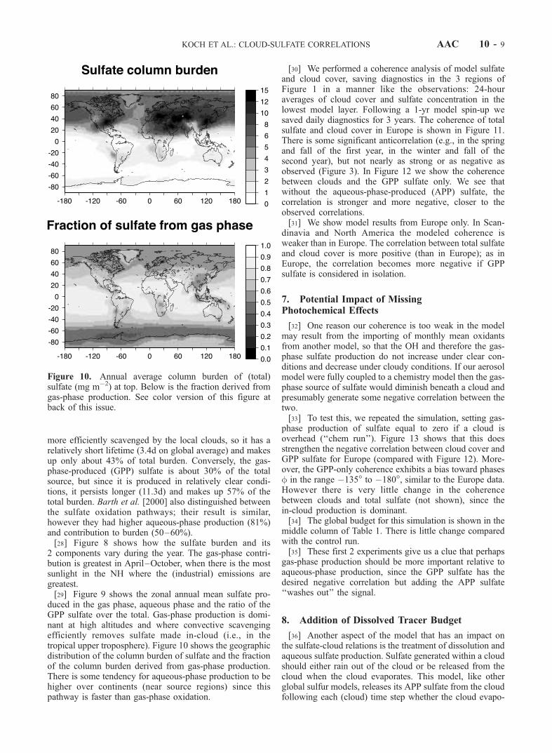
more efficiently scavenged by the local clouds, so it has arelatively short lifetime (3.4d on global average) and makesup only about 43% of total burden. Conversely, the gas-phase-produced (GPP) sulfate is about 30% of the totalsource, but since it is produced in relatively clear condi-tions, it persists longer (11.3d) and makes up 57% of thetotal burden. Barth et al. [2000] also distinguished betweenthe sulfate oxidation pathways; their result is similar,however they had higher aqueous-phase production (81%)and contribution to burden (50–60%).[28] Figure 8 shows how the sulfate burden and its

2 components vary during the year. The gas-phase contri-bution is greatest in April–October, when there is the mostsunlight in the NH where the (industrial) emissions aregreatest.[29] Figure 9 shows the zonal annual mean sulfate pro-

duced in the gas phase, aqueous phase and the ratio of theGPP sulfate over the total. Gas-phase production is domi-nant at high altitudes and where convective scavengingefficiently removes sulfate made in-cloud (i.e., in thetropical upper troposphere). Figure 10 shows the geographicdistribution of the column burden of sulfate and the fractionof the column burden derived from gas-phase production.There is some tendency for aqueous-phase production to behigher over continents (near source regions) since thispathway is faster than gas-phase oxidation.

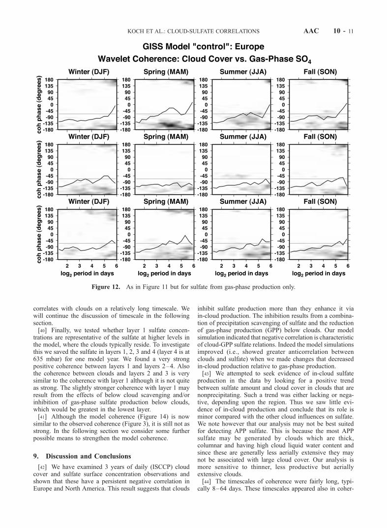
[30] We performed a coherence analysis of model sulfateand cloud cover, saving diagnostics in the 3 regions ofFigure 1 in a manner like the observations: 24-houraverages of cloud cover and sulfate concentration in thelowest model layer. Following a 1-yr model spin-up wesaved daily diagnostics for 3 years. The coherence of totalsulfate and cloud cover in Europe is shown in Figure 11.There is some significant anticorrelation (e.g., in the springand fall of the first year, in the winter and fall of thesecond year), but not nearly as strong or as negative asobserved (Figure 3). In Figure 12 we show the coherencebetween clouds and the GPP sulfate only. We see thatwithout the aqueous-phase-produced (APP) sulfate, thecorrelation is stronger and more negative, closer to theobserved correlations.[31] We show model results from Europe only. In Scan-

dinavia and North America the modeled coherence isweaker than in Europe. The correlation between total sulfateand cloud cover is more positive (than in Europe); as inEurope, the correlation becomes more negative if GPPsulfate is considered in isolation.

7. Potential Impact of MissingPhotochemical Effects

[32] One reason our coherence is too weak in the modelmay result from the importing of monthly mean oxidantsfrom another model, so that the OH and therefore the gas-phase sulfate production do not increase under clear con-ditions and decrease under cloudy conditions. If our aerosolmodel were fully coupled to a chemistry model then the gas-phase source of sulfate would diminish beneath a cloud andpresumably generate some negative correlation between thetwo.[33] To test this, we repeated the simulation, setting gas-

phase production of sulfate equal to zero if a cloud isoverhead (‘‘chem run’’). Figure 13 shows that this doesstrengthen the negative correlation between cloud cover andGPP sulfate for Europe (compared with Figure 12). More-over, the GPP-only coherence exhibits a bias toward phasesf in the range �135� to �180�, similar to the Europe data.However there is very little change in the coherencebetween clouds and total sulfate (not shown), since thein-cloud production is dominant.[34] The global budget for this simulation is shown in the

middle column of Table 1. There is little change comparedwith the control run.[35] These first 2 experiments give us a clue that perhaps

gas-phase production should be more important relative toaqueous-phase production, since the GPP sulfate has thedesired negative correlation but adding the APP sulfate‘‘washes out’’ the signal.

8. Addition of Dissolved Tracer Budget

[36] Another aspect of the model that has an impact onthe sulfate-cloud relations is the treatment of dissolution andaqueous sulfate production. Sulfate generated within a cloudshould either rain out of the cloud or be released from thecloud when the cloud evaporates. This model, like otherglobal sulfur models, releases its APP sulfate from the cloudfollowing each (cloud) time step whether the cloud evapo-

Figure 10. Annual average column burden of (total)sulfate (mg m�2) at top. Below is the fraction derived fromgas-phase production. See color version of this figure atback of this issue.


rates or not. This allows some of the sulfate to escape intothe cloud-free region of the box instead of remaining in thecloud where it more likely to be rained out.[37] To correct this, we repeated the (‘‘chem’’) simula-

tion, this time retaining APP sulfate for the duration of thecloud lifetime and releasing it into the cloudless portion ofthe box only if the cloud evaporates. As a result, the APPsulfate, now trapped in the cloud droplets, is more likely tobe scavenged. As shown in Table 1 (column 3), this causesthe APP burden and lifetime to drop to about 1/2 of theirvalues in the standard simulation; the total sulfate burdendrops by 25%. The decrease in the APP sulfate occursthroughout the troposphere (Figure 9) and, conversely, theincrease in fractional amount of GPP sulfate occursthroughout the troposphere (comparing the bottom 2 panels).Figure 8 shows that the reduction in APP sulfate occursthroughout the year.[38] Figure 14 shows that this simulation produces sig-

nificant negative coherence between cloud cover and totalsulfate over Europe for most of the seasons simulated, muchmore than in the standard simulation (Figure 11). Theimprovement was similar in North America, but less in

Scandinavia (where the APP sulfate is perhaps still toodominating). The cycle period of coherence is long, as inthe observations.[39] Since the coherence in this simulation was most like

the observations, we performed further GCM simulations toinvestigate the timescale and vertical extent of the cloudimpact on sulfate. To test whether coherence at shortertimescales would appear if our time series was saved atsmaller time steps, we saved hourly diagnostics; there wasstill no significant short period coherence. We also saved(for one year) the daily total sulfate produced and scavengedby the clouds, in order to compare with the observations andto see if a shorter timescale correlation appeared. Thesecoherences are shown (for Europe) in Figure 15. Thecorrelations for both are significant and positive. Thecoherence between clouds and sulfate deposition is strongerin the model than the observations (Figure 6) and issignificant at shorter periods than observed, though themost significant correlation is at the longer periods. Thestronger model coherence may be due to the tendency forthe model clouds to drizzle more frequently than observed.Similar to the total sulfate, daily sulfate produced in clouds

Figure 11. Coherence of modeled total sulfate and cloud cover in Europe, plotted for each season of3 years. See Figure 3 for details. On the log-period axis, 3, 4, 5, and 6 correspond to oscillation periods of8, 16, 32 and 64 days, respectively. The bars indicate our ‘‘detection level’’ for stacked coherence,estimated to be at least the 98% confidence level for nonrandomness.


correlates with clouds on a relatively long timescale. Wewill continue the discussion of timescale in the followingsection.[40] Finally, we tested whether layer 1 sulfate concen-

trations are representative of the sulfate at higher levels inthe model, where the clouds typically reside. To investigatethis we saved the sulfate in layers 1, 2, 3 and 4 (layer 4 is at635 mbar) for one model year. We found a very strongpositive coherence between layers 1 and layers 2–4. Alsothe coherence between clouds and layers 2 and 3 is verysimilar to the coherence with layer 1 although it is not quiteas strong. The slightly stronger coherence with layer 1 mayresult from the effects of below cloud scavenging and/orinhibition of gas-phase sulfate production below clouds,which would be greatest in the lowest layer.[41] Although the model coherence (Figure 14) is now

similar to the observed coherence (Figure 3), it is still not asstrong. In the following section we consider some furtherpossible means to strengthen the model coherence.

9. Discussion and Conclusions

[42] We have examined 3 years of daily (ISCCP) cloudcover and sulfate surface concentration observations andshown that these have a persistent negative correlation inEurope and North America. This result suggests that clouds

inhibit sulfate production more than they enhance it viain-cloud production. The inhibition results from a combina-tion of precipitation scavenging of sulfate and the reductionof gas-phase production (GPP) below clouds. Our modelsimulation indicated that negative correlation is characteristicof cloud-GPP sulfate relations. Indeed the model simulationsimproved (i.e., showed greater anticorrelation betweenclouds and sulfate) when we made changes that decreasedin-cloud production relative to gas-phase production.[43] We attempted to seek evidence of in-cloud sulfate

production in the data by looking for a positive trendbetween sulfate amount and cloud cover in clouds that arenonprecipitating. Such a trend was either lacking or nega-tive, depending upon the region. Thus we saw little evi-dence of in-cloud production and conclude that its role isminor compared with the other cloud influences on sulfate.We note however that our analysis may not be best suitedfor detecting APP sulfate. This is because the most APPsulfate may be generated by clouds which are thick,columnar and having high cloud liquid water content andsince these are generally less aerially extensive they maynot be associated with large cloud cover. Our analysis ismore sensitive to thinner, less productive but aeriallyextensive clouds.[44] The timescales of coherence were fairly long, typi-

cally 8–64 days. These timescales appeared also in coher-

Figure 12. As in Figure 11 but for sulfate from gas-phase production only.


ence between cloud cover and sulfate deposition. The longtimescales probably result from the fact that the sulfateconcentration in a given location is influenced by theintegration of cloud effects over a broad surrounding region,which translates into a lengthening of timescale. Further-more, the sulfate responds to the cloud systems which inturn are influenced by various intramonthly modes (e.g.,blocking episodes, index cycle, regional midlatitude wavetrains; Lanzante [1990]; Schubert [1985]). While a givensulfate particle has a relatively short lifetime (on the scale ofdays to a few weeks), the sulfate concentration level ismaintained or depleted by the ongoing production andremoval mechanisms, many of which are cloud-related.The slow shifting from cloudy to clear conditions and theresponses of the sulfate concentration and deposition areillustrated in the sample time series shown in Figure 2. Finertime-scale correlations (including evidence of in-cloudproduction) might appear if one were to observe sulfate inand around a single cloud over the course of its lifetime. Onthe larger time and spatial scales of our observations,however, only anticorrelation is preserved.[45] Our regions of study, those with daily sulfate surface

concentration measurements, were primarily located nearlarge anthropogenic source regions. The anticorrelationresult was strongest in Europe, where we also had the most

data. In Scandinavia and in the U.S., the coherence wasweaker. In Scandinavia this may be a combination of higherin-cloud production and lower gas-phase production (due tothe higher latitude). Since the North American data set isonly for one year it is difficult to speculate about ‘‘typical’’behavior there. In other regions, more remote from anthro-pogenic sources, the correlation behavior could be different.We attempted to look at data from some oceanic stations(e.g., Izana, Bermuda, Barbados; J. Prospero, private com-munication, 1997), however the data were too sparse to geta significant result.[46] We were able to use the observations to improve our

global sulfur model. Initially the model produced littlesignificant coherence between sulfate and cloud cover. Weimproved it by adding a dissolved sulfate budget, so thatsulfate generated within a cloud is not released from thecloud unless the cloud evaporates. Hence more sulfate israined out and less generated by clouds. The overall sulfateburden and lifetime are reduced by 25% (to 0.54 Tg S and4.2d, respectively). This burden is at the low end of otherglobal sulfate simulations (which range from about 0.50–0.95 Tg S). The lack of a dissolved species budget is typicalof global aerosol models. Thus we expect that other globalsulfate models would fail to generate the negative correla-tions between clouds and sulfate which appear in the

Figure 13. As in Figure 11 but for sulfate from gas-phase production only for the simulation withoutgas-phase production under clouds.


Figure 14. As in Figure 11 from the simulation with no gas phase production beneath clouds andincluding a dissolved sulfate budget.

Figure 15. Coherence of model cloud cover with daily sulfate deposition (top) and with daily sulfateproduced in-cloud (bottom). Results are from the European region.


observations. Furthermore, these models probably haveexcessive (APP) sulfate generation.[47] Although the correction of our dissolved species

scheme improved the coherence between clouds andsulfate, the resulting reduction in the sulfate burdencreates a negative bias between the modeled and observedsurface sulfate concentrations. Our standard model hadvery good agreement between model sulfate and obser-vations at the surface [Koch et al., 1999]. Now the modelis low compared with observations, especially in Europe(where it was already too low). The average model bias(model-observations/observations, where the observationsare from Koch et al. [1999]) decreases from �zero toabout ��0.3 in source regions other than Europe; inEurope it decreases from �0.3 to �0.6. However, themodel has excessive SO2 at the surface, typically doublethe observations - more than enough to fix the sulfatebias. (Our standard model performance, with minimalsulfate bias but excessive SO2, is typical of many globalsulfur models; Barrie et al. [2001]). Therefore it appearsthat another mechanism for oxidizing SO2 is required.Heterogeneous oxidation on aerosol particle surfaces,such as SO2 oxidation by ozone on dust [e.g., Usher etal., 2002] is a likely candidate: this would increasesulfate production, decrease SO{2}, and since it wouldbe most active in clear conditions it would enhance thenegative sulfate-cloud correlations.[48] Our study suggests that models ought to be pro-

ducing more sulfate in clear conditions and less in cloudyconditions. This correction is likely to have implicationsfor the indirect radiative forcing effect, since lower sulfateproduction near clouds should reduce the impact thatsulfate can have on clouds. In order to test this, werepeated our standard and ‘‘cloud budget’’ simulationsand included a simple parameterized relation betweensulfate and cloud droplet number, similar to what wasused by Menon et al. [2002] (but for sulfate only).The indirect (anthropogenic) radiative forcing decreasedonly slightly: it was �1.7 W m�2 for the standard caseand �1.5 W m�2 for the simulation with the cloudbudget. The impact on the direct anthropogenic radiativeforcing is approximately proportional to the reduction insulfate burden: the forcing decreases from �0.66 to�0.47 W m�2 for the standard and cloud-budget simu-lations, respectively. We note that including the (first)indirect effect in the simulations does not greatly affectthe cloud-sulfate correlations. The second effect (wheresulfate amount increases cloud lifetime) might, though itis likely to increase positive correlation rather thannegative correlation.[49] In addition to putting in a dissolved sulfate budget,

we were also able to improve the cloud-sulfate anticorre-lation by not allowing gas-phase sulfate productionunderneath clouds. Since our model imports its oxidantsfrom another model, these off-line fields were affected bya different model’s clouds. We tested the impact of thisby setting the gas-phase production of sulfate equal tozero if a cloud was overhead. We found that this didstrengthen the negative correlation between GPP sulfateand cloud cover. (However this improvement did notaffect the correlation between clouds and total sulfateunless the dissolved budget decreased the aqueous-phase

production relative to the gas-phase production.) Couplingthe sulfate model to a full global chemistry model mayfurther improve the anticorrelation. Since the aqueous-phase oxidant H2O2 is also affected by photochemistry(due to its photolysis, relation to OH, etc.), such couplingmay impact the correlations for both phase-productionpathways.[50] In conclusion, we encourage the use of the observed

anticorrelation between sulfate and clouds as a diagnostictest for global sulfate models. Furthermore, global aerosoland chemistry models need to verify that they are handlingdissolution and evaporation correctly: that the dissolvedspecies are only released from clouds as they evaporate.Fixing this in our model caused the ratio of the GPPsulfate burden to APP sulfate burden to increase from 1.3to 2.

[51] Acknowledgments. This work was supported by the NASAGlobal Aerosol Climatology Program. J. Park was supported by NOAAgrant Y770995. The EMEFS data utilized in this study were collected andprepared under the cosponsorship of the United States EnvironmentalProtection Agency, the Atmospheric Environment Service, Canada, theOntario Ministry of Environment, the Electric Power Research Institute,and the Florida Electric Power Coordinating Group.

ReferencesBarrie, L. A., et al., A comparison of large-scale atmospheric sulfate aerosolmodels (COSAM): Overview and highlights, Tellus, Ser. B, 53, 615–645,2001.

Barth, M. C., P. J. Rasch, J. T. Kiehl, C. M. Benkovitz, and S. E. Schwartz,Sulfur chemistry in the National Center for Atmospheric Research Com-munity Climate Model: Description, evaluation, features, and sensitivityto aqueous chemistry, J. Geophys. Res., 105, 1387–1415, 2000.

Bear, L. K., and G. L. Pavlis, Multi-channel estimation of time residualsfrom broadband seismic data using multi-wavelets, Bull. Seismol. Soc.Am., 89, 681–692, 1999.

Chin, M., R. B. Rood, S.-J. Lin, J.-F. Muller, and A. Thompson, Atmo-spheric sulfur cycle simulated in the global model GOCART: Modeldescription and global properties, J. Geophys. Res., 105, 24,671 –24,687, 2000.

Koch, D., D. Jacob, I. Tegen, D. Rind, and M. Chin, Tropospheric sulfursimulation and sulfate direct radiative forcing in the Goddard Institute forSpace Studies general circulation model, J. Geophys. Res., 104, 23,799–23,822, 1999.

Lanzante, J., The leading modes of 10–30 day variability in the extratropicsof the Northern Hemisphere during the cold season, J. Atmos. Sci., 47,2115–2140, 1990.

Lilly, J., and J. Park, Multiwavelet spectral and polarization analysis ofseismic records, Geophys. J. Int., 122, 1001–1021, 1995.

Lohmann, U., and G. Lesins, Stronger constraints on the anthropogenicindirect aerosol effect, Science, 298, 1012–1015, 2002.

McNaughton, D. J., and R. J. Vet, Eulerian model evaluation field study(EMEFS): A summary of surface network measurments and data quality,Atmos. Environ., 30, 227–238, 1996.

Menon, S., A. D. Del Genio, D. Koch, and G. Tselioudis, GCM simulationsof the aerosol indirect effect: Sensitivity to cloud parameterization andaerosol burden, J. Atmos. Sci., 59, 692–713, 2002.

Park, J., and M. E. Mann, Interannual temperature events and shifts inglobal temperature: A multiwavelet correlation approach, Earth Interact.,4, online paper 4-0001, 2000.

Park, J., F. L. Vernon III, and C. R. Lindberg, Frequency-dependent polar-ization analysis of high-frequency seismograms, J. Geophys. Res., 92,12,664–12,674, 1987a.

Park, J., C. R. Lindberg, and F. L. Vernon III, Multitaper spectral analysis ofhigh frequency seismograms, J. Geophys. Res., 92, 12,675–12,684,1987b.

Penner, J. E., et al., Aerosols: Their direct and indirect effects, in ClimateChange 2001: The Scientific Basis, edited by J. T. Houghton et al.,pp. 289–348, Cambridge Univ. Press, New York, 2001.

Percival, D. B., and A. T. Walden, Spectral Analysis for Physical Applica-tions, Cambridge Univ. Press, New York, 1993.

Rossow, W. B., and R. A. Schiffer, Advances in understanding clouds fromISCCP, Bull. Am. Meteorol. Soc., 80, 2261–2288, 1999.

Schaug, J., J. E. Hansen, K. Nodop, B. Ottar, and J. M. Pacyna, Summaryreport from the chemical co-ordinating center for the third phase of


EMEP, EMEP/CC Rep. 3/87, 160 pp., Norw. Inst. for Air Res., Lilles-trom, 1987.

Schubert, S. D., A statistical-dynamical study of empirically determinedmodes of atmospheric variability, J. Atmos. Sci., 42, 3–17, 1985.

Schwartz, S. E., Harshvardhan, and C. M. Benkovitz, Influence of anthro-pogenic aerosol on cloud optical depth and albedo shown by satellitemeasurements and chemical transport modeling, Proc. Nat. Acad. Sci.,99, 1784–1789, 2002.

Stubenrauch, C. J., W. B. Rossow, F. Cheruy, A. Chdin, and N. A., Cloudsas seen by satellite sounders (3I) and imagers (ISCCP). Part I. Evaluationof cloud parameters, J. Clim., 12, 2189–2213, 1999.

Thomson, D. J., Spectrum estimation and harmonic analysis, IEEE Proc.,70, 1055–1096, 1982.

Usher, C. R., H. Al-Hosney, S. Carlos-Cuellar, and V. H. Grassian, Alaboratory study of the heterogeneous uptake and oxidation of sulfurdioxide on mineral dust particles, J. Geophys. Res., 107(D23), 4713,doi:10.1029/2002JD002051, 2002.

��A. Del Genio and D. Koch, NASA Goddard Institute for Space Studies,

Columbia University, 2880 Broadway, New York, NY 10025, USA.([email protected])J. Park, Department of Geology and Geophysics, Yale University,

P.O. Box 208109 New Haven, CT 06520-8109, USA. ( [email protected])


Figure 9. Zonal annual mean of the gas-phase produced sulfate, aqueous-produced sulfate, and gas-phase divided by the total sulfate for the standard run (1st column) and the cloud budget run (2ndcolumn). The concentrations unit is ng m�3.

KOCH ET AL.: CLOUD-SULFATE CORRELATIONS

AAC 10 - 8

Figure 10. Annual average column burden of (total) sulfate (mg m�2) at top. Below is the fractionderived from gas-phase production.

KOCH ET AL.: CLOUD-SULFATE CORRELATIONS

AAC 10 - 9

clouds and sulfate are anticorrelated: a new diagnostic

Documents