Climate Variability, Child Labour and

Schooling: Evidence on the Intensive and

Extensive Margin

Jonathan Colmer

September 2013

Centre for Climate Change Economics and Policy Working Paper No. 148

Grantham Research Institute on Climate Change and the Environment

Working Paper No. 132

The Centre for Climate Change Economics and Policy (CCCEP) was established by the University of Leeds and the London School of Economics and Political Science in 2008 to advance public and private action on climate change through innovative, rigorous research. The Centre is funded by the UK Economic and Social Research Council and has five inter-linked research programmes:

1. Developing climate science and economics 2. Climate change governance for a new global deal 3. Adaptation to climate change and human development 4. Governments, markets and climate change mitigation 5. The Munich Re Programme - Evaluating the economics of climate risks and

opportunities in the insurance sector More information about the Centre for Climate Change Economics and Policy can be found at: http://www.cccep.ac.uk. The Grantham Research Institute on Climate Change and the Environment was established by the London School of Economics and Political Science in 2008 to bring together international expertise on economics, finance, geography, the environment, international development and political economy to create a world-leading centre for policy-relevant research and training in climate change and the environment. The Institute is funded by the Grantham Foundation for the Protection of the Environment and the Global Green Growth Institute, and has five research programmes:

1. Global response strategies 2. Green growth 3. Practical aspects of climate policy 4. Adaptation and development 5. Resource security

More information about the Grantham Research Institute on Climate Change and the Environment can be found at: http://www.lse.ac.uk/grantham. This working paper is intended to stimulate discussion within the research community and among users of research, and its content may have been submitted for publication in academic journals. It has been reviewed by at least one internal referee before publication. The views expressed in this paper represent those of the author(s) and do not necessarily represent those of the host institutions or funders.

Climate Variability, Child Labour and

Schooling: Evidence on the Intensive

and Extensive Margin1

Jonathan ColmerLondon School of Economics

Abstract

How does future income uncertainty affect child labour and human capital

accumulation? Using a unique panel dataset, we examine the effect of changes

in climate variability on the allocation of time among child labour activities

(the intensive margin) as well as participation in education and labour activ-

ities (the extensive margin). We find robust evidence that increased climate

variability increases the number of hours spent on farming activities while re-

ducing the number of hours spent on domestic chores, indicating a substitution

of time across child labour activities. In addition, we find no evidence of cli-

mate variability on enrolment decisions or educational outcomes, suggesting

that households may spread the burden of labour across children to minimise

its impact on formal education.

(JEL: D13, O12, J13, J22, Q54.)

1First draft: June 2012. Colmer: Grantham Research Institute and Department of Geography andEnvironment, London School of Economics, Houghton Street, London, WC2A 2AE, UK. E-mail address:j.m.colmer@lse.ac.uk. I am grateful to Gharad Bryan, Antoine Dechezlepretre, Jon de Quidt, Greg Fisher,Maitreesh Ghatak, Ben Groom, Sol Hsiang, Rob Jensen, Kyle Meng, Anthony Millner, Eric Neumayer,Munir Squires and seminar audiences at the London School of Economics, Columbia University, the EfD 6thAnnual Meeting, the 20th Annual Conference of the European Association of Environmental and ResourceEconomics, and the European Economic Association, for helpful thoughts, comments and discussions. Thiswork was supported by the ESRC Centre for Climate Change Economics and Policy and the GranthamFoundation. The data used in this article were collected by the University of Addis Ababa, the InternationalFood Policy Research Institute (IFPRI), and the Centre for the Study of African Economies (CSAE). Fundingfor the ERHS survey was provided by the Economic and Social Research Council (ESRC), the SwedishInternational Development Agency (SIDA) and the United States Agency for International Development(USAID). All errors and omissions are my own.

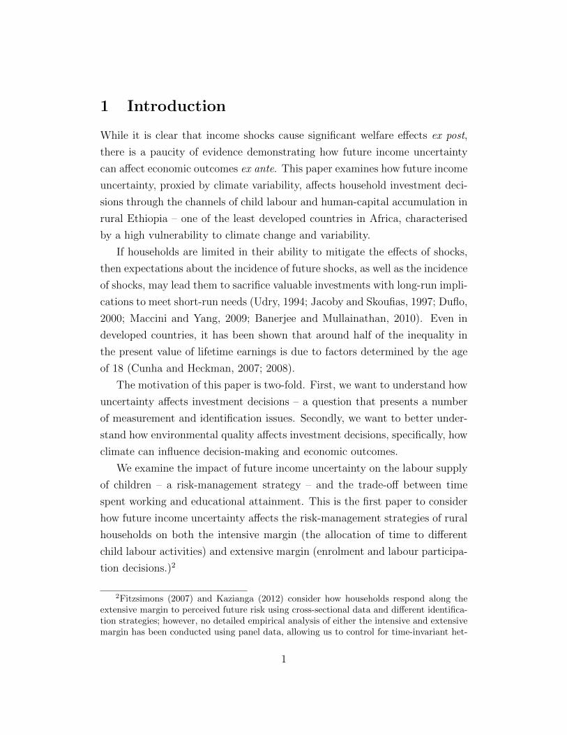
1 Introduction

While it is clear that income shocks cause significant welfare effects ex post,

there is a paucity of evidence demonstrating how future income uncertainty

can affect economic outcomes ex ante. This paper examines how future income

uncertainty, proxied by climate variability, affects household investment deci-

sions through the channels of child labour and human-capital accumulation in

rural Ethiopia – one of the least developed countries in Africa, characterised

by a high vulnerability to climate change and variability.

If households are limited in their ability to mitigate the effects of shocks,

then expectations about the incidence of future shocks, as well as the incidence

of shocks, may lead them to sacrifice valuable investments with long-run impli-

cations to meet short-run needs (Udry, 1994; Jacoby and Skoufias, 1997; Duflo,

2000; Maccini and Yang, 2009; Banerjee and Mullainathan, 2010). Even in

developed countries, it has been shown that around half of the inequality in

the present value of lifetime earnings is due to factors determined by the age

of 18 (Cunha and Heckman, 2007; 2008).

The motivation of this paper is two-fold. First, we want to understand how

uncertainty affects investment decisions – a question that presents a number

of measurement and identification issues. Secondly, we want to better under-

stand how environmental quality affects investment decisions, specifically, how

climate can influence decision-making and economic outcomes.

We examine the impact of future income uncertainty on the labour supply

of children – a risk-management strategy – and the trade-off between time

spent working and educational attainment. This is the first paper to consider

how future income uncertainty affects the risk-management strategies of rural

households on both the intensive margin (the allocation of time to different

child labour activities) and extensive margin (enrolment and labour participa-

tion decisions.)2

2Fitzsimons (2007) and Kazianga (2012) consider how households respond along theextensive margin to perceived future risk using cross-sectional data and different identifica-tion strategies; however, no detailed empirical analysis of either the intensive and extensivemargin has been conducted using panel data, allowing us to control for time-invariant het-

1

Our results add to the growing literature exploring climatic influence on

economic outcomes (Barreca et al. 2013; Burgess et al. 2011; Deschenes and

Greenstone, 2007; 2011; 2012; Dell, Jones and Olken, 2009; 2012; Fischer et

al., 2012; Graff Zivin and Neidell, 2010; Graff Zivin et al., 2013; Guiteras, 2009;

Hsiang, 2010; Schlenker and Roberts, 2009) as well as the literature looking

at the impacts of risk on educational outcomes (Fitzsimons, 2007; Kazianga,

2012).

Using two rounds of individual-level panel data, combined with a new data

set of village-level meteorological data, we exploit exogenous variation in future

income uncertainty to examine the relationship between climate variability and

child labour.

We observe that an increase in future income uncertainty results in a sub-

stitution of child labour across activities, from labour in the home to labour on

the farm, i.e., adjustment on the intensive margin. However, in contrast to the

previous literature examining the effects of ex ante risk on human capital in-

vestments (Fitzsimons, 2007; Kazianga, 2012), we find no evidence to suggest

that climate variability decreases the likelihood that children attend school or

affects educational attainment, indicating the potential for omitted-variable

bias due to unobserved individual heterogeneity. We demonstrate the impor-

tance of controlling for time-invariant omitted variables through replicating

the results of these previous studies using individual cross-sections.

Our results can be interpreted as causal effects, conditional on the assump-

tion that our measure of climate variability affects child labour and schooling

only through uncertainty about future states of the world. In order to support

this assumption, we show that our results are robust to controlling for past and

contemporaneous rainfall shocks and other time-varying factors which may be

correlated with our measure of income uncertainty, as well as time-invariant

unobserved heterogeneity at the village level. Alem and Colmer (2013) also

demonstrate rigorous evidence supporting the plausibility of this measure in

an examination of the impact of income uncertainty on experienced utility in

rural Ethiopia.

erogeneity.

2

We also present the results from a series of placebo and robustness tests

used to disentangle the effect from other confounding factors and provide sup-

porting evidence for the main identification assumption.3

This narrative is distinct from the literature, which has focussed on child

labour and reductions in human capital investments as an ex post response to

adverse shocks (Jacoby & Skoufias, 1997; Jensen, 2000; Portner, 2001; Ranjan,

2001; Sawada & Lokshin, 2001; Bhalotra & Heady, 2003; Thomas et al., 2004;

Beegle et al., 2006). The decision to withdraw children from school, most

frequently observed in response to adverse shocks, may arise from a need to

reduce expenditures; it is less likely that there would be an increase in child

labour due to reductions in the marginal product of labour. If there is an

increase in child labour it is likely to be off-farm and so may result in an

increase in child labour supply along the extensive margin ,i.e., the decision

to engage in work outside of the home.

The remainder of the paper is organised as follows: section 2 provides a

brief background and literature review; section 3 presents a simple theoretical

model which supports and motivates our findings; section 4 provides a brief

summary of the data along with caveats; section 5 describes our empirical

specification and outlines our identification strategy; section 6 presents the

main results and a discussion of the implications; section 7 reports supporting

evidence and robustness checks; section 8 concludes.

2 Background

In a recent publication, the World Bank (2010) argues that climate change

will disproportionately affect poor households, especially women and children.

Children may be withdrawn from school in response to climatic shocks, with

long-run and irreversible impacts on human capital and, consequently, lifetime

earnings. In addition, while the majority of child labour is at home, off-farm

3Appendix C provides a number of more mechanical robustness tests, which help supportthe statistical and economics significance of the results but matter less for supporting theidentification assumptions made.

3

child labour is very responsive to negative income shocks.4 There is little

evidence, however, on the role that income uncertainty plays in education and

child labour decisions. Uncertainty in climate patterns can pose a serious

threat to agricultural productivity (Cline, 2007; Easterling et al., 2007) and

place increased pressure on household responsibilities and activities. There is

considerable evidence from Asia to show that delays and variation in the timing

of the wet season can have significant productivity impacts; the evidence in

Africa, mainly due to data limitations, is more scarce.

Developing countries are especially vulnerable to climate change: they are

more physically exposed as a result of their location in the Tropics and other

areas that are regularly subjected to extreme weather events, such as storms,

droughts, flooding, and extreme temperatures; they are more economically

sensitive, due to weak infrastructure and heavy reliance on agriculture; they

also have a lower adaptive capacity, resulting from institutional and governance

factors.

In the face of uninsured risk, households that are subject to greater vari-

ability have a greater incentive to accumulate precautionary savings to smooth

consumption against future risk (Kimbell,1991; Paxson, 1992; Carroll, 1997;

Carroll & Kimbell, 2001). The pivotal result in this literature states that, in

the presence of uninsured risk, prudent households are likely to save more than

in the absence of uncertainty. The existing literature focuses on the effects of

income uncertainty on consumption and asset portfolios. One channel through

which this effect may be observed, first discussed by Cain (1982), and more

recently discussed in Fitzsimons (2007), is not to enrol children in school.5 Ed-

ucation is an irreversible investment with delayed, and potentially increasing,

marginal returns. Fafchamps and Pender (1997) further argue that the precau-

tionary motive for holding liquid assets impedes productive investment, such

as investments in education, even if households are able to self-finance them.

As a result, it is argued that the effect of the precautionary motive on irre-

4Unfortunately, there is not sufficient data to examine the effect of shocks on wagelabour carried out by children.

5It is assumed that children would engage in child labour in place of this activity, thoughit is possible that children may remain idle.

4

versible and illiquid investments, such as education, is augmented. There are

two mechanisms which can be explored here. The first mechanism arises from

the decision not to enrol children in school to increase saving through reduced

educational expenditures, as discussed above, with an assumed increase in the

labour supply of children along the extensive margin, or increased idleness.

The second mechanism results from a risk-management and productivity mo-

tive by which households may invest more in the land, taking more care over

the land-preparation and cultivation stages in efforts to reduce the likelihood

of crop failure in the event of an adverse shock. This mechanism works along

the intensive margin of labour supply. The question that remains is whether

an increase in labour supply along the intensive margin is sufficient to also

affect decisions on the extensive margin. It is assumed that parents optimally

invest in the number and quality of children, determined by investments in

human capital, to maximise household welfare. Under this assumption, Fitzsi-

mons (2007) argues that children have an instantaneous earnings potential in

addition to the benefit of reduced educational expenditures. Consequently, we

might expect that higher levels of risk should result in a greater incentive to

increase the number of hours worked by children and reduce investments in

education.

If this risk results in reduced investment in human capital then the po-

tential welfare cost may have long-run welfare costs via worsened later-life

outcomes and opportunity (Strauss and Thomas, 1998; Maccini and Yang,

2009; Banerjee et al., 2010; Antilla-Hughes & Hsiang, 2013). Indeed, even de-

lays in educational attainment may have large effects if children are not able

to reach a level of education that has real returns. These costs may be fur-

ther exacerbated if households reduce investments in children based on gender

(Sen, 1990; Duflo, 2005; Antilla-Hughes and Hsiang, 2013).

However, in many studies, this study included, we observe children are

capable of both working and attending school.6 Ravallion and Wodon (2000)

argue that poor families can protect the schooling of working children because

675% of our sample both attend school and work, either on the farm or in the home.49% attend school and work on the farm. 59% attend school and work in the home.

5

there are other things that children do besides school and work.

“One cannot assume that the time these children spend working must come

at the expense of formal time at school, although there may be displacement of

informal (after-school) tutorials or homework.”

Jayachandran (2013) demonstrates, however, that the displacement of in-

formal schooling may have significant welfare effects of its own. If schools offer

for-profit tutoring to their own students, this gives teachers a perverse incen-

tive to teach less during school to increase demand for tutoring. Consequently,

those who do not participate in tutoring could be adversely affected.

This paper explores whether uncertainty about future income is enough

to displace investment in education. We argue that, while the realisation of

income shocks may result in the withdrawal of children from school, it is likely

that households are able to reallocate time across activities and children to

minimise the effect on education. If this is the case, we would expect to observe

an increase in child labour on the intensive margin (the loss-minimisation

motive) but no enrolment effects on the extensive margin (the precautionary

savings motive). Whether there is an effect on educational attainment depends

on whether there is a large enough impact on the intensive margin of education

(unobserved in the data) or whether informal education in the form of tutoring

is an important determinant, as in Jayachandran (2013).7

3 Theoretical Framework

To motivate our empirical work and demonstrate the plausibility of our find-

ings, we introduce a two-period model of the child labour supply decision in

agricultural households in the spirit of Rose (2001). The two-period frame-

7Ideally, test scores would provide a more accurate measure of educational attainment.To observe an impact on the grades attained there would have to be sufficient impact inorder to stop schooling, or to not progress to the next year.

6

work allows for explicit consideration of ex ante and ex post decisions.8 In

both periods, the household makes decisions regarding the time-allocation of

children between labour supply on the farm, in the home, and schooling. Time-

allocation is normalised to 1. The first period is characterised as prior to the

realisation of rainfall. This could be seen as the cultivation and land prepara-

tion stages of agriculture. In the second period, rainfall is realised, and again

households respond to this through the time-allocation decision, conditional

on the decision in period 1. Figure 1 provides a graphical representation of

the model.

In period 1, the household does not know how much rainfall, ξ, there will

be, but does know its distribution. The household knows the average level of

rainfall over time for the area (µ), and knows the variability of the distribution

measured as the coefficient of variation (ϕ), the standard deviation divided by

the mean. In this respect, the coefficient of variation could be seen as the

probability of a shock occurring in period 2. The household’s time-allocation

decision for the first period depends on µ and ϕ, in addition to household

wealth, Y, the shadow price of the activity, ωi, and the parameters of the

production technology, θ.

In each period, time can be allocated to labour on the farm, domestic

chores, or schooling.9

The ex ante labour supply on the farm is:

LF1 = LF

1 (µ, ϕ, ωF ,Y, θ)

8This paper focusses on ex ante decisions. As already mentioned, there is a considerableliterature that has focussed on ex post responses to adverse shocks (Jacoby & Skoufias, 1997;Jensen, 2000; Portner, 2001; Ranjan, 2001; Sawada & Lokshin, 2001; Bhalotra & Heady,2003; Thomas et al., 2004; Beegle et al., 2006). The results presented in the second periodof this model are consistent with the results in this literature.

9Allowing for an additional dimension, idleness, changes none of the results in the model.For clarity, we restrict our analysis to the three dimensions discussed.

7

The ex ante labour supply in the home is:

LH1 = LH

1 (µ, ϕ, ωH ,Y, θ)

The ex ante investment in education is:

E1 = E1(µ, ϕ, ωE,Y, θ) = 1− LF1 − LH

1

There are two channels by which we might expect ϕ to affect these deci-

sions. First, there is a “portfolio effect” whereby, given the shadow price of an

activity, the household will adjust the time-allocation of children away from

risky activities on the farm towards less risky investments in schooling and in

the home. The second effect results from a precautionary motive. Prior to

the realisation of a shock, households may allocate more time to labour on

the farm to mitigate the effects of a shock in the event that it is realised. If

the precautionary effect dominates the portfolio effect, we would expect the

following:

∂LF1

∂ϕ> 0,

∂LH1

∂ϕ< 0,

∂E1

∂ϕ< 0

In this case, an increase in risk, ϕ, will increase child labour supply on

the farm, reduce child labour supply in the home, and reduce investment in

education.

By contrast, if the portfolio effect dominates, then we would expect:

∂LF1

∂ϕ< 0,

∂LH1

∂ϕ> 0,

∂E1

∂ϕ> 0

In this case, an increase in risk, ϕ, will reduce child labour supply on the

farm, increase child labour supply in the home, and increase investment in

education.

In period 2, the value of rainfall, ξ, is realised, and households can respond

to it. Conditional on labour supply in period 1, there is no reason for ϕ to

affect household decision-making once ξ is realised. Consequently, the ex post

labour supply decision for farming is:

8

LF2 = LF

2 (LF1 (·), µ, ε, ωF ,Y, θ)

The ex post labour supply in the home is:

LH2 = LH

2 (LH1 (·), µ, ε, ωF ,Y, θ)

The ex post investment in education is:

E2 = E2(E1(·), µ, ε, ωE,Y, θ) = 1− LF2 − LH

2

where ε = ξ − µ, i.e., ε is the deviation in rainfall from the mean.

The effect of ε on time allocation can be separated into an income effect

and a substitution effect. If the realisation of rainfall is below average (ε is

low), then income is lower and the household may need to withdraw children

from school to smooth income (the income effect); however, if the returns to

education (child labour on the farm) are decreasing (increasing) as ε increases,

then we would expect an increase (decrease) in schooling (child labour on the

farm) following a negative shock (the substitution effect). In the literature

which has examined ex post responses to adverse shocks through education

and child labour, the income effect has consistently been shown to dominate

the substitution effect at low income levels. The remainder of this paper

attempts to tackle the question of ex ante decision making in the context of

child labour and education, motivated by the hypotheses presented in this

model.

4 Data

The analysis conducted in this paper uses two rounds of the Ethiopian Rural

Household Survey collected by the University of Addis Ababa, the Centre for

the Study of African Economics (CSAE) at the University of Oxford, and the

International Food Policy Research Institute (IFPRI), covering 15 communi-

9

ties in rural Ethiopia.10 This paper makes use of the latest two rounds of this

panel from 2004 and 2009. These years are included as they contain consis-

tent identifiers of child labour across time and are the only years to contain

individual-level identifiers, allowing us to track children across the rounds.11

The villages in the survey represent the diversity of farming systems through-

out Ethiopia and capture climate differences across the country. Stratified

random sampling is used within each village, based on whether households

have male or female heads.

The survey has several features that make it appropriate for the analysis.

The main attraction is its detailed information on individuals and the house-

hold, including time spent in the previous week working on the farm and in

the home. Furthermore, the sample is widely representative of rural Ethiopia,

giving it common support. That said, there are several concerns that arise

from the use of the survey. The first is attrition, which is a problem with all

panel data sets. However, attrition in the ERHS has been limited at 1–2% of

households per year (Dercon and Hoddinott, 2009). Nevertheless, if children

or households were to exit (or enter) the sample in a way that was correlated

with rainfall or climate variability, this would bias our results. A second con-

cern is the small number of clusters in the context of village-level analysis. We

bootstrap-cluster our standard errors of our regressions to account for this. A

final concern is that the survey design includes an over-sample of households

considered to be at risk. This is unlikely to be too great a problem, however,

as weather is random and the survey covers a wide geographic area.

Table 1 reports the means and standard deviations of the variables used in

the analysis.

10See figure 3 in appendix A for the location of these villages11The total survey consists of 7 rounds between 1989 and 2009. In 1989, households from

six villages in central and southern Ethiopia were interviewed. In 1994, however, the samplewas expanded to cover 15 villages across the country, representing 1477 households. Furtherrounds were completed in 1995, 1997, 1999, 2004 and 2009.

10

Table 1: Summary statistics

Variable Mean Std. Dev. N

Dependent Variables

Child labour hours (total) 27.55 16.71 4034

Child labour hours (farm) 13.93 15.17 4015

Child labour hours (domestic) 13.73 12.85 4019

Child labour participation (total) 0.96 0.17 4034

Child labour participation (farm) 0.65 0.47 4034

Child labour participation (domestic) 0.75 0.42 4034

Idle 0.01 0.11 4034

Not Attending 0.10 0.29 4034

Discontinued 0.03 0.18 4034

Zero Grades 0.16 0.37 4034

Primary School Completed 0.09 0.29 4034

Climate Variables

Climate Variability (annual) 22.91 4.44 4034

Negative Rainfall Shock (past 5 years) 0.69 0.46 4034

Individual Characteristics

Male 0.52 0.49 3726

Age child 10.89 2.94 4034

Youngest child 0.35 0.47 4034

Grades (head) 1.53 2.83 4034

Grades (spouse) 0.72 1.82 4034

Household Characteristics

Days worked off-farm 11.56 27.06 4034

Remittances received (birr) 134.12 1066.59 4034

Land (hectares) 1.36 1.95 3603

In the analysis on the intensive margin, child labour – the dependent vari-

able – is defined as the total hours spent working in economic activities and

chores per week. We define children to be aged between 6 and 16, consistent

with the literature. This is also consistent with the starting age of school in

Ethiopia so as not to amplify any effect of variability on enrolment in school.

Economic activities generally consist of farming activities, including tending

crops, processing crops, looking after livestock, etc. Chores are also included

for two reasons. First, child labour is not restricted to economic activities.

Second, in rural areas it may be difficult to distinguish between time spent

on household chore activities and time spent preparing subsistence food crops.

From table 1 we can see that the average number of hours spent per week

on all child labour is just under 30 hours per week. This is a considerable

11

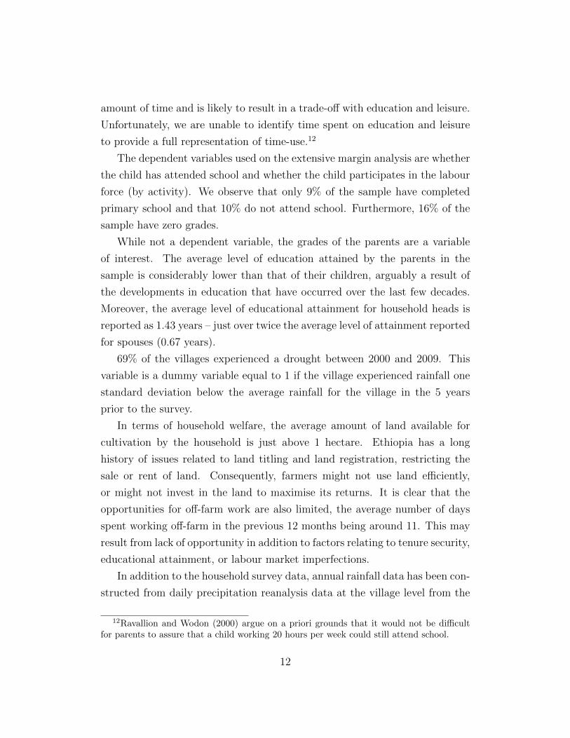
amount of time and is likely to result in a trade-off with education and leisure.

Unfortunately, we are unable to identify time spent on education and leisure

to provide a full representation of time-use.12

The dependent variables used on the extensive margin analysis are whether

the child has attended school and whether the child participates in the labour

force (by activity). We observe that only 9% of the sample have completed

primary school and that 10% do not attend school. Furthermore, 16% of the

sample have zero grades.

While not a dependent variable, the grades of the parents are a variable

of interest. The average level of education attained by the parents in the

sample is considerably lower than that of their children, arguably a result of

the developments in education that have occurred over the last few decades.

Moreover, the average level of educational attainment for household heads is

reported as 1.43 years – just over twice the average level of attainment reported

for spouses (0.67 years).

69% of the villages experienced a drought between 2000 and 2009. This

variable is a dummy variable equal to 1 if the village experienced rainfall one

standard deviation below the average rainfall for the village in the 5 years

prior to the survey.

In terms of household welfare, the average amount of land available for

cultivation by the household is just above 1 hectare. Ethiopia has a long

history of issues related to land titling and land registration, restricting the

sale or rent of land. Consequently, farmers might not use land efficiently,

or might not invest in the land to maximise its returns. It is clear that the

opportunities for off-farm work are also limited, the average number of days

spent working off-farm in the previous 12 months being around 11. This may

result from lack of opportunity in addition to factors relating to tenure security,

educational attainment, or labour market imperfections.

In addition to the household survey data, annual rainfall data has been con-

structed from daily precipitation reanalysis data at the village level from the

12Ravallion and Wodon (2000) argue on a priori grounds that it would not be difficultfor parents to assure that a child working 20 hours per week could still attend school.

12

ERA-Interim data archive supplied by the European Centre for Medium-Term

Weather Forecasting (ECMWF).13 Where previous studies have relied on the

use of meteorological data provided by the Ethiopian meteorological service,

the number of missing observations, or observations which are recorded as zero

on days when there are no records, is of concern. The ERA-Interim reanal-

ysis data archive provides daily measurements of precipitation, temperature

(min, max, and mean), wind speed and wind direction, relative humidity, cloud

cover (a proxy for solar reflectance), and many other atmospheric parameters,

from January 1st 1979 until the present day, on a global grid of quadrilateral

cells defined by parallels and meridians at a resolution of 0.75 x 0.75 degrees

(equivalent to 83km x 83km at the equator).14 Reanalysis data is constructed

through a process whereby model information and observations are combined

to produce a consistent global best estimate of atmospheric parameters over

a long period of time by optimally fitting a dynamic model to each period si-

multaneously (Auffhammer et al., 2013). Models propagate information from

areas with more observational data for areas in which observational data are

scarce. This results in an estimate of the climate system that is separated

uniformly across a grid, that is more uniform in its quality and realism than

observations alone, and that is closer to the state of existence than any model

would provide alone. This provides a consistent measure of atmospheric pa-

rameters over time and space. This type of data is increasingly being used by

economists (see Burgess et al., 2011; Guiteras, 2009; Hsiang et al., 2011; Ku-

damatsu, 2012; Schlenker & Lobell, 2010), as they fill in the gap in developing

countries, where the collection of consistent weather data is lower down the

priority list in government budgets.

By combining the ERHS data set with the ERA-interim data, we create

a unique panel allowing for microeconomic analysis of weather and climate in

Ethiopia.

It is important to note that all climate data, whether reanalysis or observa-

13See Dee et al. (2011) for a detailed discussion of the ERA-Interim data.14To convert degrees to km, multiply 83 by the cosine of the latitude, e.g. at 40 degrees

latitude 0.75 x 0.75 cells are 83 x cos(40) = 63.5 km x 63.5 km.

13

tional data, are subject to caveats and concerns. Reanalysis data is unlikely to

match observational data perfectly. It is limited to some degree by resolution,

even where observational data is present. Furthermore, reanalysis data are

partly computed using climate models that are imperfect and contain system-

atic biases. This brings up further concern to issues of accuracy. However,

in areas with limited observational data such as Ethiopia, reanalysis data is

known to provide estimates that are better than they otherwise could be, be-

cause the data is collected at intervals of six hours, over which time weather

follows physical laws in an almost linear fashion.

There are statistical reasons as to why reanalysis data may be preferable.

Previous studies have relied on the use of meteorological data provided by the

Ethiopian meteorological service and the number of missing observations is a

concern. This is exacerbated by the serious decline in the past few decades in

the number of weather stations around the world that are reporting. Lorenz

and Kuntsman (2012) show that since 1990 the number of reporting weather

stations in Africa has fallen from around 3,500 to around 500. With 54 coun-

tries in the continent, this results in an average of fewer than 10 weather sta-

tions per country. Looking at publicly available data, the number of stations in

Ethiopia included by the National Oceanic and Atmospheric Administration’s

(NOAA) National Climatic Data Centre (NCDC) is 18; however, if we were

to apply a selection rule that required observations for 365 days this would

yield a database with zero observations. For the two years for which we have

economic data (2004 and 2009), weather station data is available for 50 days

from one station (Addis Ababa) in 2004 and is available for all 18 stations

for an average of 200 days (minimum of 67 days, maximum of 276 days) in

2009. This is likely to result in a huge increase in measurement error when

this data is used to interpolate across the 63 zones and 529 woredas (districts)

reported in 2008. If this measurement error is classical, i.e., uncorrelated with

the actual level of rainfall measured, then our estimates of the effect of these

variables will be biased towards zero. However, given the sparse density of sta-

tions across ethiopia (an average of 0.03 stations per woreda), the placement

of stations is likely to be correlated with agricultural output, i.e., weather sta-

14

tions are placed in more agriculturally productive areas, where the need for

weather information is greater.

Rainfall at each village is calculated by taking data points within 100km of

the village and then interpolated through a process of inverse distance weight-

ing. Taking the annual measure of rainfall at each village, we calculate the

coefficient of variation for rainfall, measured as the standard deviation divided

by the mean for the periods 1995–2004 and 2000–2009.

We focus on rainfall data for our measures of village risk and shocks, as the

data is both spatially and temporally rich, providing an exogenous measure

over a long period of time that is ideal for working with longitudinal data.

While weather events and shocks are not the only exogenous factor influenc-

ing variability in agricultural output and income, it is arguably the factor that

contributes the most to income fluctuations, leading to welfare changes (Bin-

swanger and Rosenzweig, 1993). This is especially true of Ethiopia, where

agriculture accounts for such a large proportion of GDP and employment.

Furthermore, it is important to gain a better understanding of the impact of

weather risk and shocks on behaviour and decision-making, given the risks

that climate change poses to many developing countries. This is key to under-

standing how current development policy is compatible with adaptation needs

in response to climate change, and where gaps in policy arise.

Table 2 reports the mean rainfall for each village for each year of the panel,

and the mean, standard deviation and coefficient of variation over the entire

period.

15

Table 2: Annual Rainfall (mm) by Peasant Authority and Year

Peasant Association 2004 2009 mean std. dev. CV

Haresaw 395 470 476 155 33.12

Geblen 226 261 278 95 34.24

Dinki 810 865 853 162 18.61

Yetmen 667 713 740 149 20.00

Shumsheha 535 627 645 150 23.34

Sirbana Godeti 1150 1218 1086 172 15.61

Adele Keke 1175 1169 1008 177 17.19

Korodegaga 1478 1589 1364 218 15.6

Turfe Kechemane 1170 1177 1024 197 18.86

Imbidir 1051 1062 936 158 16.68

Aze Deboa 1232 1253 1073 210 19.08

Addado 1258 1399 1188 305 25.29

Gara Godo 1546 1520 1318 271 20.16

Doma 1134 1270 1070 257 23.71

Debre Berhan Villages 838 893 855 154 17.53

The mean, std. dev. and CV are calculated for the period 1980-2009.

Rainfall is low and erratic in Ethiopia. From table 2, we observe that there

is considerable variability across the villages as well as between years. The

average across all the villages is just under 1000mm per annum, but there is

considerable heterogeneity. For example, Haresaw and Geblen, villages from

the Tigray region in northern Ethiopia, experienced on average 400mm per

annum between 1980 and 2009. Figure 1 in appendix A provides a visualisation

of the inter-annual heterogeneity in rainfall, as well as a demonstration of the

degree to which the villages in the sample represent the average climate of

Ethiopia. Figure 2 in appendix A shows density plots for the coefficient of

variation over the two periods for which we have economic data, demonstrating

the temporal variation we observe, even in a short time frame. Figures 4 and 5

in the appendix provide a visualisation of the spatial heterogeneity in average

rainfall and variability.

16

5 Empirical Specification and Identification

Strategy

This paper investigates how future income uncertainty, drawn from historical

rainfall variability, affects child labour and human capital accumulation on

the intensive and extensive margin. We employ the coefficient of variation in

rainfall (hereafter CV), measured as the standard deviation of rainfall divided

by the mean for the previous ten years, as an exogenous determinant of the

level of risk that households face. Unlike the variance or standard deviation of

rainfall, the CV is scale invariant, providing a comparable measure of variation

for households that may have very different income levels (Fitzsimons, 2007).15

Using these measures, we examine the impact of climate variability on

child labour hours (the intensive margin), the probability that children attend

school, educational attainment (measured as grades attained), and the prob-

ability that the children participate in labour activities (the extensive mar-

gin). We use the difference-in-means estimation approach (i.e., fixed-effects

or “within” regression), which allows us to address the issue of time-invariant

unobserved heterogeneity, captured by village fixed effects.

The use of cross-sectional data does not address this issue, leading to po-

tential omitted-variable bias due to time-invariant unobserved heterogeneity

correlated with the treatment effect or the dependent variable. Examples of

this unobserved heterogeneity in the context of our paper might include the

geography of the village, access to markets, infrastructure such as schools and

roads, and access to insurance against covariate shocks, such as food for work

programmes.

In addition to village fixed effects, we control for year fixed effects to control

for aggregate shocks, economic development, and macroeconomic policies. We

also include month fixed effects to control for any seasonal variation in the

timing of the survey. Fitzsimons (2007) argues that it is not unrealistic to

imagine that households in riskier villages have lower preferences for education;

15It is important to note that our results are robust to using the standard deviation ofrainfall and other time measures of the CV.

17

however, unlike Fitzsimons (2007), who uses a cross-sectional instrumental

variable approach, we are able to control for these factors. Indeed, it is well

established that family preferences for education are a major determinant of

educational attainment (Heckman, 2007; 2008).

A main concern surrounding the empirical specification of the model is the

number of zeros in the child labour data, as it implies that the dependent

variable is not normally distributed, leading to inconsistent and inefficient

estimates under the Gaussian assumptions of linear regression. To account for

the large number of zeroes in the dependent variables, we estimate a fixed-

effects Poisson Quasi-Maximum Likelihood Estimator model (QMLE)16 with

cluster-robust Huber-White standard errors at the village level to account for

serial correlation within villages. 17

The model is estimated using the following specification:

E(yihvt) = µv(exp(βcvvt + φX′iht + αt + αm) (1)

where subscripts index individuals (i), households (h), village (v) and year

(t).18 yihvt corresponds to the number of child labour hours for child i in

household h (located in village v) in year t. CVvt corresponds to the coefficient

of variation at the village level, our measure of village risk. In addition to these

core variables, we include a set of controls and characteristics, X, measured

at the individual, household, and village level. µv corresponds to the village

fixed effects and αt to the year fixed effects. We interpret the β coefficients

in equation 4 as the semi-elasticity of child labour (or grades attained) in

response to a unit change in the variable.

As the village-level fixed effect (µv) is multiplicative to the rainfall vari-

ables, this makes households with higher levels of child labour more responsive

16See Hausman et al. (1984), Wooldridge (1999; 2010) for an introduction to the model,and Burgess et al. (2011) and Vanden Eynde (2011) for recent applications. See Santos Silvaand Tenreyro (2006) for an evaluation of the differences between OLS and QMLE Poisson.

17Our results are robust to OLS specifications in logs and levels, presented in appendixB.

18For the analysis of enrolment and labour force participation, we estimate fixed-effectslinear probability models.

18

to climate variability or shocks. As a result, the fixed effects explain all the

variation in households that do not have any child labour, therefore these

households do not contribute towards the estimation of the β coefficients.

There are a number of benefits to using the Poisson QMLE instead of the

standard Poisson MLE. For example, the use of the QMLE does not require

that the data follow a Poisson distribution. All that is required is that the

conditional mean of the variable of interest be correctly specified. A further

benefit in the context of Poisson models is the mitigation of concerns surround-

ing under- and over-dispersion. This is because, unlike the MLE, the Poisson

QMLE does not assume equi-dispersion. All that is required for optimality

of the Poisson QMLE is that the conditional variance is proportional to the

conditional mean. Furthermore, the Poisson QMLE will still be consistent in

the case where the conditional variance is not proportional to the conditional

mean. This means that we can work using a fixed-effects framework without

needing to use models such as the negative-binomial or zero-inflation Poisson

MLE to deal with consistency issues.

Due to the grouped nature of our data, it is likely that the standard errors

will be underestimated, resulting in overstated t-statistics. We account for

this by clustering the standard errors by group, i.e., at the village level. The

importance of clustering is emphasised by Moulton (1986; 1990), and more

recently by Bertrand, Duflo and Mullainathan (2004). We cluster at the village

level in line with Pepper (2002) and Bertrand et al. (2004), who argue that

one should cluster at the highest level where there may be correlation. In our

context, we are examining individuals, in a household, which is part of the

larger village community. As the variation in climate is measured for each

village, we want to cluster at this level.

However, Bertrand, Duflo and Mullainathan (2004), Angrist and Pischke

(2009) and Cameron, Gelbach and Miller (2008) show that when group size

is below 30 clusters, asymptotic tests can over-reject the null hypothesis. As

a consequence, the use of block bootstrap methods to account for cluster-

ing at the village level results in more consistent estimators and asymptotic

refinement.

19

In addition to concerns about the empirical specification, there are a num-

ber of caveats related to the data and identification strategy that need to be

discussed and, where possible, addressed.

A general concern is measurement error, especially considering the retro-

spective nature of the survey methods used (Deaton, 1997). This may be a

particular issue regarding the dependent variable, which measures the number

of hours of child labour. For example, there may be general reporting error

due to recall, or hours at lower levels of work being rounded up, e.g., 30 mins

becomes one hour. It may also be the case that richer, more educated house-

holds deliberately under-report child labour due to a greater understanding

of the stigma attached. While this should not bias the results, if we believe

that this measurement error is classical, and that any non-classical measure-

ment error is fixed over time, it could increase the size of the standard errors,

increasing the risk of type II errors in which we fail to reject the null hypoth-

esis. Given cultural attitudes towards child labour, however, it is likely that

concerns about stigma are less than in other contexts.

While measurement error in the dependent variable is possible, this is less

of a concern than in the main explanatory variable, CV, which would lead to

inconsistent estimation and downward-biased estimates of β1. We minimise

classical measurement error associated with self-reported data by using the

CV, which is measured using quality-controlled meteorological data, as a direct

measure of income risk, rather than using an instrumental variable approach,

as in Fitzsimmons (2007). However, all meteorological data is measured with

some error and so we expect our coefficients to be a lower-bound estimate.

The use of rainfall variables has become increasingly popular in economics

as a means of identifying permanent and transitory components of income,

as well as income variability. The main advantages of rainfall as a proxy

or as an instrumental variable are its strong correlation with income and its

presumably random variation. This variation is presumed to be orthogonal

to other unobserved determinants of income, offering a potential solution to

omitted-variable bias problems. In effect, it is argued that rainfall has no

effect on the dependent variable other than through income. Indeed, the key

20

identifying assumption of this paper is that historical climate variability is

exogenous to recent child labour and educational decisions, i.e., the only way

in which rainfall has an effect on child labour and educational decisions is

through village risk.

However, the effect of weather on permanent and transitory income are

based on theoretical frameworks with strong assumptions about the operation

of rural labour and land markets, preferences, and technology. Rosenzweig

and Wolpin (2000) argue that the assumption of orthogonality with other un-

observed determinants may be overly strong. This is a concern noted in Fitzsi-

mons (2007), and also aired here. While a fixed-effects estimation approach

controls for time-invariant omitted variables, we are still concerned about time-

variant omitted variables that may impact child labour and schooling decisions

and are also correlated with our measure of income risk. For example, rain-

fall shocks may have resulted in disasters that caused damage to schools or

infrastructure, directly affecting school attendance and child labour decisions.

As a result of this, we control for whether the village has experienced a rain-

fall shock in the previous five years. We are confident with this measure as,

unlike other studies in which the data on shocks is subject to the caveat that

it is self-reported, our measure is based on a quality-controlled meteorological

measurement.

On a similar note, past rainfall may have affected the labour market de-

cisions of other household members, leading to off-farm labour supply as an

attempt to diversify the income portfolio. To control for this, we include

whether household members are engaged in off-farm labour, measured as the

number of days worked off-farm in the previous 12 months. However, due to

labour market imperfections or general equilibrium effects, this may not be an

effective method of diversifying risk. For example, Jayachandran (2006) shows

that productivity shocks depress wages by more when workers are poorer, less

able to migrate, and more credit-constrained because of the inelasticity of these

workers’ labour supply. Macours et al. (2012) conducted a randomized control

trial in Nicaragua and found that a conditional cash transfer allowed house-

holds in rural areas to diversify out of agriculture, increasing mean income by

21

8% and increasing resilience to droughts.

It is more likely that past rainfall may have affected the labour market de-

cisions of household members through the channel of migration or by marrying

off family members to other villages in order to diversify covariate risk. Indeed,

Rosenzweig and Stark (1989) show that marriage with migration significantly

reduces the variation in household food consumption and that households sub-

ject to more variable income tend to engage more in longer-distance marriage

with migration. In relation to labour market decisions, Bryan, Chowdhury

and Mobarak (2012) randomly assign a small cash transfer, equivalent to the

cost of travel, to out-migrate during the famine season in Bangladesh. They

report that this transfer induces 22% of households to send a family member

to migrate, that consumption of the family members with a migrant increases

by 30%, and that the effect of this one-time transfer is persistent with posi-

tive spillover effects: the migration rate is 10 percentage points higher in year

2, and 8 percentage points higher in year 3. We control for these potential

factors as much as we can through the remittances received by the household.

In addition, strong regionalisation in Ethiopia means it is very difficult to ob-

tain work outside of your locality, this further mitigates such concerns about

migration behaviour.

6 Results and Discussion

In this section we present and discuss the results, examining the effect of

climate variability on child labour (total, farming, and domestic chores) and

educational outcomes (whether the children have enrolled).

6.1 Child Labour: The Intensive Margin

The effects of climate variability on the number of hours worked by children

is estimated using the difference-in-means fixed-effects framework through the

Poisson QMLE model.

Turning first to table 3, we examine the effects of climate variability on

22

the number of hours worked using the specification from equation (4). We ob-

serve that an increase in weather risk increases the number of hours worked in

farming and decreases the number of hours worked in the home. This results

in the net effect of weather risk on child labour being zero. This is demon-

strated in column 3, which examines total child labour. This emphasises the

importance of looking at the effect or risk on child labour activities separately,

in order to observe substitution of labour across activities. Given the small

number of clusters observed in our data set (15 villages) we bootstrap-cluster

the standard errors in order to provide the most robust classification of the

standard errors. This is important as it is more likely that the null hypothesis

will be rejected when the number of clusters is small.

Following the discussion at the end of section 5, we interpret these results

as the semi-elasticity of child labour in response to a unit change in an ex-

planatory variable. The Poisson QMLE fixed-effects model is non-linear, and

so these results are dependent on the coefficient and on the expected value of

the number of hours worked, conditional on the coefficient. Consequently, the

larger the value of E(y|x), the larger the rate of change in E(y|x).

23

Table 3: Number of Hours Worked by Children

(1) (2) (3)

Child Labour Child Labour Child Labour

(Farm) (Home) (Total)

Climate Variability 0.0406*** -0.0291*** 0.00814

(0.0128) (0.00667) (0.00774)

Rainfall Shock (past 5 years) -0.000899 0.0383 0.0242

(0.0874) (0.0338) (0.0522)

Male 1.070*** -0.946*** 0.0358

(0.0825) (0.109) (0.0312)

Age 0.104** 0.150*** 0.129***

(0.0420) (0.0345) (0.0164)

Age2 -0.00427** -0.00514*** -0.00478***

(0.00182) (0.00160) (0.000717)

Grades (Head) 0.00481 -0.00600 -0.00155

(0.00751) (0.0110) (0.00750)

Grades (Spouse) -0.0116 -0.00898 -0.00905

(0.0123) (0.0104) (0.00875)

Log Remittances -0.00927 0.0109 0.00132

(0.00608) (0.00698) (0.00335)

Log Days Worked Off-Farm -0.0129 -0.0130 -0.00922

(0.00828) (0.0122) (0.00787)

Land (Hectares) 0.0283** 0.00133 0.0137

(0.0141) (0.00735) (0.00840)

Fixed Effects Yes Yes Yes

Observations 3,212 3,213 3,222

Log-Likelihood -25,145.945 -20,179.375 -21,639.531

Notes: Fixed effects: Village, Year, Season (Month). Significance levels are indi-

cated as * 0.10 ** 0.05 *** 0.01. Standard errors are bootstrap clustered at the

village level (1000 replications) to account for heteroskedasticity and clustering at

the village level in addition to concerns over the small number of clusters.

We observe that a one-unit increase in the CV is associated with a 4%

increase in the number of hours worked on the farm. Referring to table 1, a

one standard deviation change in the CV is 4.44 units. As such, a one standard

deviation change in the CV is associated with a 17.76 percentage point increase

in the number of hours worked on the farm. To give more structure to the

interpretation of this effect, we compare the difference across villages using the

24

values provided in table 2. We see that the community with the smallest CV

is Korodegaga (15.60), and the village with the largest CV is Geblen (34.24).

From the results in table 3, we might expect that the average level of farming

child labour in Geblen is 62.4% higher than in Korodegaga.19 We observe

that, for domestic child labour, a one-unit increase in the CV results in a

2.9% decrease in child labour in the home. This is especially interesting, as

it indicates that there is some substitution between activities in response to

increased variability, emphasising the importance of measuring child labour

based on different activities as opposed to aggregate measures, as discussed

in Beegle et al. (2006). Climate variability may result in more work in the

planting and cultivation stages of agriculture in order to minimise losses in the

event of a shock: an increase in the intensive margin of labour supply. A one

standard deviation change in the CV is associated with a 12.7% decrease in

the number of hours worked in the home. Furthermore, a comparison between

Geblen and Korodegaga reveals that, on average, the expected level of child

labour in the home is 54.05% less in Korodegaga.

With regard to the other coefficients, we see that age has a significant posi-

tive effect on the level of child labour across all activities, but at a diminishing

rate. This may be an indication of the increasing productivity of children in

the home (due to child-care responsibilities increasing with age) and on the

farm (due to increased productivity on manual tasks as children develop).

In addition to age effects, we observe significant gender effects. The number

of hours worked in farming is increasing for boys, while decreasing in domestic

chores by a similar magnitude. This indicates that households may allocate

tasks in accordance with potential comparative advantages.

While these results are reduced-form and do not indicate the precise mech-

anism through which climate variability increases child labour on the farm,

our results indicate that it may have a significant impact on household time-

allocation decisions. The fact that climate variability has an effect on the

number of hours of child labour indicates, from our theoretical framework,

that households may invest more child labour in farming to minimise losses in

19(34.24 - 15.6) x 0.04 = 0.624

25

the event of a shock. To understand whether this is merely a change in the

intensive margin of child labour supply, with time being allocated differently

across activities without a reduction in education on the extensive margin,

we must understand the effects of climate variability on enrolment and labour

force participation.

6.2 School and Labour Force Participation:

The Extensive Margin

From a policy perspective, part of the concern related to child labour relates

to the degree that it crowds out educational attainment. As we have observed,

climate variability is associated with an increase in child labour on the farm,

and a decrease in child labour in the home. Given this substitution, it is of

interest to understand whether there are also changes on the extensive margin.

An increase in participation, above and beyond the changes in the intensive

margin, may have an impact on education if the substitution of activities on the

intensive margin is not able to account for the full adjustment. In examining

the effects of climate variability on education, we first explore whether climate

variability increases the probability that children participate in child labour

activities and whether it increases the likelihood that these children either do

not attend or delay entry into school, as discussed by Fitzsimons (2007) and

Kazianga (2012)).

Table 4 presents results from linear probability models examining the im-

pact of climate variability on participation in child labour on the farm, in the

home, and whether the child participates in any child labour.

26

Table 4: Participation in child labour activities - the extensive margin

(1) (2) (3)

Child Labour (Farm) Child Labour (Home) Child Labour (Total)

Climate Variability 0.0165** -0.00336 -0.000786

(0.00783) (0.00866) (0.00246)

Rainfall Shock (past 5 years) -0.00187 -0.0657 0.0132

(0.0336) (0.0520) (0.0154)

Male 0.391*** -0.326*** -0.0221***

(0.0211) (0.0362) (0.00490)

Age 0.0509*** 0.0509** 0.0544***

(0.0157) (0.0231) (0.0104)

Age2 -0.00209*** -0.00212** -0.00225***

(0.000705) (0.000989) (0.000439)

Grades (Head) 0.0146*** 0.00584* 0.00117

(0.00379) (0.00331) (0.00123)

Grades (Spouse) 0.00000907 -0.00132 0.00186

(0.00962) (0.00386) (0.00120)

Log Remittances -0.00567 0.00743*** 0.00163

(0.00556) (0.00262) (0.00129)

Log Days Worked Off-Farm -0.00392 -0.00695 0.000673

(0.00600) (0.00430) (0.00269)

Land (Hectares) 0.00983** -0.00279 -0.000141

(0.00443) (0.00584) (0.00133)

Fixed Effects Yes Yes Yes

Observations 3222 3222 3222

Adjusted R2 0.180 0.166 0.023

Notes: Fixed effects: Village, Year, Season (Month). Significance levels are indicated as * 0.10 ** 0.05

*** 0.01. Standard errors are bootstrap clustered at the village level (1000 replications) to account for

heteroskedasticity and clustering at the village level in addition to concerns over the small number of

clusters.

We observe that there is very little impact on the extensive margin other

than for child labour on the farm. This indicates that most of the adjustment

takes place on the intensive margin, i.e., that households are able to substitute

time across activities.

In examining the effect of risk on the propensity to not attend or delay

entry into school, we present results from linear probability models (table 5).

27

Table 5: Education, Education, Education - the extensive margin

(1) (2) (3) (4)

Not Attending Never Attended Zero Grades Grades Completed

Climate Variability -0.00460 0.00272 -0.00824 -0.0207

(0.00989) (0.00176) (0.0117) (0.0787)

Rainfall Shock (past 5 years) 0.0271 -0.0234 -0.0109 -0.162

(0.0604) (0.0163) (0.0786) (0.383)

Male 0.000895 -0.00111 -0.0170 0.0447

(0.00963) (0.00716) (0.0278) (0.141)

Age -0.0644*** -0.00228 -0.144*** 0.704***

(0.0165) (0.00513) (0.0172) (0.0859)

Age2 0.00214*** 0.0000797 0.00522*** -0.00966**

(0.000583) (0.000245) (0.000674) (0.00394)

Grades (Head) 0.00114 -0.000899 -0.00594 0.0637***

(0.000977) (0.000587) (0.00419) (0.0169)

Grades (Spouse) -0.00856*** -0.00114 -0.0139*** 0.0803***

(0.00265) (0.00107) (0.00255) (0.0284)

Log Remittances -0.00214 0.000364 -0.00123 -0.0153

(0.00139) (0.00140) (0.00316) (0.0274)

Log Days Worked Off-Farm 0.00407 0.00210 0.00253 -0.0419

(0.00336) (0.00167) (0.00461) (0.0342)

Land (Hectares) 0.00476 -0.00246 0.00180 0.00681

(0.00506) (0.00217) (0.00460) (0.0326)

Fixed Effects Yes Yes Yes Yes

Observations 2959 2484 3222 3222

Adjusted R2 0.070 -0.004 0.123 0.399

Notes: Fixed effects: Village, Year, Season (Month). Significance levels are indicated as * 0.10 ** 0.05

*** 0.01. Standard errors are bootstrap clustered at the village level (1000 replications) to account for

heteroskedasticity and clustering at the village level in addition to concerns over the small number of

clusters.

Table 5 shows that we are unable to reject the null hypothesis that cli-

mate variability has no effect on the decision to enrol children in school, nor

on educational attainment. This is plausible given the adjustment along the

intensive margin. In addition, as argued by Fitzsimons (2007), this could in-

dicate that households in riskier villages have lower preferences for education,

which is captured by the village fixed effects. If we restrict the sample to be

28

cross-sectional (for 2004 or 2009) we are able to replicate the results observed

in Fitzsimons (2007), i.e., that the variability decreases the probability that

children attend school. We present these cross-sectional results in table 6.

Table 6: Education, Education, Education - the extensive margin (Cross-section)

(1) (2) (3) (4)

(2004) (2009) (2004) (2009)

Zero Grades Zero Grades Grades Attained Grades Attained

Climate Variability -0.00560 -0.0285*** 0.258*** 0.172***

(0.00612) (0.00717) (0.0556) (0.0284)

Rainfall Shock (past 5 years) – 0.0618 – -0.610**

(0.0513) (0.292)

Village Dummies Yes Yes Yes Yes

Month Dummies Yes Yes Yes Yes

Observations 1615 1607 1615 1607

Adjusted R2 0.077 0.321 0.402 0.496

Notes: In 2004 village shocks in the previous 5 years was omitted as all villages had experienced at

least one shock. All regressions include same controls as table 3. Significance levels are indicated as *

0.10 ** 0.05 *** 0.01. Standard errors are bootstrap clustered at the village level (1000 replications) to

account for heteroskedasticity and clustering at the village level in addition to concerns over the small

number of clusters.

While there is little evidence to support the impact of climate variability

on enrolment, there may be an impact on the intensive margin. It is likely to

be the case that time is allocated away from informal educational experiences

such as homework and out-of-school tutoring. However, without data on time

allocation within education, we cannot estimate the elasticity of education

with respect to child labour to evaluate a precise trade-off.

7 Supporting Evidence

In order to demonstrate the robustness of the results, we consider a number

of additional extensions and robustness checks to try to validate our measure

of climate variability and isolate the channel observed in the reduced form

29

results. In appendix C, we present additional mechanical robustness checks

and stress tests.

7.1 Spreading the Burden

First, we test our hypothesis that households spread the burden of labour

across children. If we believe that the households’ utility is increasing in

education, then it is also possible that they may try to smooth the burden

of child labour across children to mitigate the impact on education. This

might explain in part why we observe no average effect of climate variability

on enrolment.

We explore this potential in a number of ways. First, we look at the

degree to which the opportunity of spreading the burden across children is

available to households by looking at interactions between whether the child

has any siblings and climate variability. Although we note that family size

is endogenous in this context and, as such, cannot be argued to be causal, it

does help to motivate the narrative. In order to deal with this endogeneity

issue, we also examine the interaction between climate variability and being

the eldest child. While the number of children is endogenous, sibling order is

not. The argument made to support this channel is based on the idea that

at the time when decisions about educating the eldest child were being made,

there was no substitute child labour available and so consequently the burden

of labour fell on the eldest child. This allows for multiple sibling families, but

accounts for the fact that younger siblings would not have engaged in child

labour, or would not have been productive in the same way at such a young

age.

We first report the results on the number of siblings and then the results

on sibling order. We test the first hypothesis by interacting climate variability

with a dummy variable equal to one if the child has no siblings and zero if the

child has one or more siblings.

As we observe in table 7, while climate variability itself is insignificant, the

interaction term is significant at the 1% level. From column (1), we observe

30

that if a child has no siblings, then a one standard deviation increase in the

coefficient of variation (4.44) increases the probability that the child does not

attend school by 2.2 percentage points. As above, if we compare Geblen and

Korodegaga, we observe that the probability of not attending school is just

over 9% more likely in Geblen if a child has zero siblings relative than if a

child has one or more siblings. In terms of educational attainment, we observe

from column (4) that a one standard deviation increase in the coefficient of

variation (4.44) reduces grade attainment by 0.2 grades. In comparing Geblen

and Korodegaga, we observe a reduction in grades close to 1 (0.85). While this

does not seem like a particularly large effect, we argue that this is the impact

of uncertainty, not the realisation of a shock.

Table 7: Education, Education, Education - Sibling Interaction

(1) (2) (3) (4)

Not Attending Never Attended Zero Grades Grades Completed

Climate Variability -0.00553 0.00207 -0.00219 0.00830

(0.0106) (0.00134) (0.00789) (0.0669)

No Siblings -0.132*** -0.0804*** -0.115* 0.943**

(0.0411) (0.0279) (0.0635) (0.475)

Climate Variability × No Siblings 0.00509*** 0.00301*** 0.00452* -0.0457**

(0.00164) (0.00105) (0.00231) (0.0179)

Fixed Effects Yes Yes Yes Yes

Observations 2,959 2,747 3,222 2,959

Adjusted R2 0.071 -0.003 0.045 0.415

Notes: Fixed effects: Village, Year, Season (Month). Significance levels are indicated as * 0.10 ** 0.05 *** 0.01.

All regressions include same controls as table 3. Standard errors are bootstrap clustered at the village level

(1000 replications) to account for heteroskedasticity and clustering at the village level in addition to concerns

over the small number of clusters.

As discussed, we try to deal with the potential endogeneity concerns by

considering interactions with the ordering of children. The following table

examines the interaction between climate variability and being the eldest child.

31

Table 8: Education, Education, Education - Eldest Child Interaction

(1) (2) (3) (4)

Not Attending Never Attended Zero Grades Grades Completed

Climate Variability -0.00923 0.00120 -0.0124 -0.00715

(0.0103) (0.00190) (0.0117) (0.0773)

Eldest -0.255*** -0.0899*** -0.218** 0.745

(0.0658) (0.0262) (0.102) (0.561)

Climate Variability × Eldest 0.00961*** 0.00335*** 0.00882** -0.0290

(0.00259) (0.000986) (0.00396) (0.0224)

Fixed Effects Yes Yes Yes Yes

Observations 2959 2484 3222 3222

Adjusted R2 0.079 0.000 0.126 0.399

Notes: Fixed effects: Village, Year, Season (Month). Significance levels are indicated as * 0.10 ** 0.05 ***

0.01. All regressions include same controls as table 3. Standard errors are bootstrap clustered at the village

level (1000 replications) to account for heteroskedasticity and clustering at the village level in addition to

concerns over the small number of clusters.

From table 8, we observe again that, while we cannot reject the null hy-

pothesis that climate variability has no effect on educational outcomes, the

interaction with a dummy variable, equal to one if the child is the eldest sib-

ling, and zero otherwise, is significant at the 1% level. From column (1), we

observe that if a child is the eldest sibling, then a one standard deviation in-

crease in the coefficient of variation (4.44) increases the probability that the

child does not attend school by 4.2 percentage points. As above, if we com-

pare Geblen and Korodegaga, we observe that the probability of not attending

school is just over 17.9% more likely in Geblen if a child is the eldest sibling.

While the channel through which this effect occurs is not conclusive (it

could simply be the case that elder children are more productive and so are

more likely to be used in child labour), this evidence, in addition to the results

on the number of siblings, is supportive of an argument in which households

spread the burden of labour across children.

32

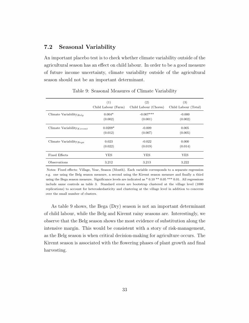
7.2 Seasonal Variability

An important placebo test is to check whether climate variability outside of the

agricultural season has an effect on child labour. In order to be a good measure

of future income uncertainty, climate variability outside of the agricultural

season should not be an important determinant.

Table 9: Seasonal Measures of Climate Variability

(1) (2) (3)

Child Labour (Farm) Child Labour (Chores) Child Labour (Total)

Climate VariabilityBelg 0.004* -0.007*** -0.000

(0.002) (0.001) (0.002)

Climate VariabilityKiremt 0.0209* -0.009 0.005

(0.012) (0.007) (0.005)

Climate VariabilityBega 0.023 -0.022 0.000

(0.022) (0.019) (0.014)

Fixed Effects YES YES YES

Observations 3,212 3,213 3,222

Notes: Fixed effects: Village, Year, Season (Month). Each variable corresponds to a separate regression

e.g. one using the Belg season measure, a second using the Kiremt season measure and finally a third

using the Bega season measure. Significance levels are indicated as * 0.10 ** 0.05 *** 0.01. All regressions

include same controls as table 3. Standard errors are bootstrap clustered at the village level (1000

replications) to account for heteroskedasticity and clustering at the village level in addition to concerns

over the small number of clusters.

As table 9 shows, the Bega (Dry) season is not an important determinant

of child labour, while the Belg and Kiremt rainy seasons are. Interestingly, we

observe that the Belg season shows the most evidence of substitution along the

intensive margin. This would be consistent with a story of risk-management,

as the Belg season is when critical decision-making for agriculture occurs. The

Kiremt season is associated with the flowering phases of plant growth and final

harvesting.

33

8 Conclusions

The objective of this paper was to evaluate the extent to which future in-

come uncertainty, proxied by climate variability, influences household decision-

making in the context of child labour and human capital accumulation. We

observe that climate variability has a significant effect on the number of hours

that children work on the farm (the intensive margin), with substitution of

time from child labour in the home to child labour on the farm. Contrary to

previous research, there is no effect of climate variability on enrolment in school

or educational attainment. The only effect we find on the extensive margin is

that children are more likely to participate in child labour on the farm. This

may be motivated by households’ efforts to spread the burden across children

to reduce the impact on education and leisure. This mechanism is supported

by results which indicate that increased climate variability decreases the prob-

ability that children attend school for children with no siblings. This channel

is further supported by examining the interaction between climate variability

and sibling order, to deal with endogeneity concerns surrounding family size

and child labour.

Results on the intensive margin of child labour supply indicate that in-

creased climate variability increases the number of hours worked on the farm

with decreases in the number of hours worked in the home. This indication

of substitution between activities emphasises the importance of distinguish-

ing between activities when examining the determinants of child labour, as

discussed by Beegle et al. (2006). We argue that households form expecta-

tions about the likelihood of future income shocks based on the variability of

the climate. We posit that, in order to manage this risk, households increase

child labour on the farm ex ante to minimise losses in the event that income

shocks should occur in the future. This hypothesis, supported by our results,

contrasts with recent work by Fitzsimons (2007) and Kazianga (2012), who

argue that households do not enrol children in school in an ex ante response

to future income risk, as a precautionary savings mechanism. We show that

the results from these studies are likely to be the artefact of the cross-sectional

34

data used. However, this is not to say that climate variability has no effect

on human capital accumulation. Without time-allocation data on education,

we are unable to observe the effects of increased child labour on the amount

of time spent in school and on more informal educational investments, such as

homework and external tutoring, which may limit participation in education

at later levels.

These results emphasise the importance of understanding ex ante as well

as ex post responses to fully understand the risk-management practices of

households. While this paper focusses on a representative sample of rural

Ethiopia, we are not able to examine the effects of weather risk in urban

areas, as in Fitzsimons (2007). Consequently, our conclusions may have limited

external validity to Ethiopia as a whole; however, it is unlikely that urban areas

will be affected by future income uncertainty, proxied by climate variability, as

shown in Alem and Colmer (2013). Overall, the results suggest that climate

variability may be an important factor in household decisions related to child

labour and investment in human capital, pointing to the need for more research

into the socio-economic impacts of climate change across a broad range of

economic and policy contexts.

References

Alem, Y. and J. Colmer (2013). Optimal expectations and the welfare cost of

climate variability: A subjective well-being approach. Grantham Research

Institute Working Paper Series No. 118 .

Angrist, J. and J. Pischke (2009). Mostly Harmless Econometrics: An Em-

piricist’s Companion. Princeton University Press, Princeton, N.J., USA.

Antilla-Hughes, J. and S. Hsiang (2013). Destruction, disinvestment, and

death: Economic and human losses following environmental disaster.

Mimeo.

Auffhammer, M., S. Hsiang, W. Schlenker, and A. Sobel (2013). Using weather

35

data and climate model output in economic analyses of climate change.

Review of Environmental Economics nad Policy .

Banerjee, A. and S. Mullainathan (2010). The shape of temptation: Implica-

tions for the economic lives of the poor. NBER Working Paper No. 15973 .

Barreca, A., K. Clay, O. Deschenes, M. Greenstone, and J. Shapiro (2013).

Adapting to climate change: The remarkable decline in the u.s. temperature-

mortality relationship over the 20th century. NBER Working Paper 18692 .

Beegle, K., R. H. Dehejia, and R. Gatti (2006, October). Child labour and

agricultural shocks. Journal of Development Economics 81 (1), 80–96.

Bertrand, M., E. Duflo, and S. Mullainathan (2004). How much should we trust

difference-in-difference estimates? Quarterly Journal of Economics 119,

249–275.

Bhalotra, S. and Heady (2003). Child farm labor: The wealth paradox. World

Bank Economic Review 17 (2), 197–227.

Binswanger, H. and M. Rosenzweig (1993). Wealth, weather risk and the

composition and profitability of agricultural investments. Economic Jour-

nal 103 (416), 56–78.

Bryan, G., S. Chowdhury, and A. Mobarak (2012). Migrating away from a

seasonal famine: A randomized intervention in bangladesh. Mimeo.

Burgess, R., O. Deschenes, D. Donaldson, and M. Greenstone (2011). Weather

and death in india. Mimeo.

Burgess, R., M. Hansen, B. Olken, P. Potapov, and S. Sieber (2011). The

political economy of deforestation in the tropics. NBER Working Paper No.

17417 .

Cain, M. (1982). Perspectives on family and fertility in developing countries.

Population Studies 36 (2), 159–175.

36

Cameron, C., J. Gelbach, and D. Miller (2008). Bootstrap-based improvements

for inference with clustered errors. Review of Economics and Statistics 90,

414–427.

Carroll, C. (1997). Buffer-stock saving and the life cycle/permanent income

hypothesis. Quarterly Journal of Economics 107 (1), 1–55.

Carroll, C. and M. Kimball (2001). Liquidity constraints and precautionary

saving. Working Paper 2001 Johns Hopkins University .

Cline, W. (2007). Global Warming and Agriculture: Impact Estimates by

Country. Global Development and the Peterson Institute for Interational

Economics, Washington D.C.

Cunha, F. and J. Heckman (2007). The evolution of inequality, heterogeneity

and uncertainty in labor earnings in the u.s. economy. NBER Working

Papers No. 13526 .

Cunha, F. and J. Heckman (2008). A new framework for the analysis of

inequality. Macroeconomic Dynamics 12 (2), 315–354.

Deaton, A. (1997). Analysis of Household Surveys: A Microeconomic Approach

to Development Policy. John Hopkins University Press.

Dee, D. P., S. M. Uppala, A. J. Simmons, P. Berrisford, P. Poli, S. Kobayashi,

U. Andrae, M. A. Balmaseda, G. Balsamo, P. Bauer, P. Bechtold, A. C.

Beljaars, L. M., van de Berg, J. Bidlot, N. Bormann, C. Delsol, R. Dragani,

M. Fuentes, A. J. Geer, L. Haimberger, S. B. Healy, H. Hersbach, E. V.

Holm, L. Isaksen, P. Kallberg, M. Kohler, M. Matricardi, A. P. McNally,

B. Monge-Sanz, J. Morcrette, B. Park, C. Peubey, P. de Rosnay, C. Tavolato,

J. Thepaut, and F. Vitart (2011). The era-interim reanalysis: configuration

and performance of the data assimilation system. Quarterly Journal of the

Royal Meteorological Society 137, 553–597.

37

Dell, M., B. Jones, and B. Olken (2009). Temperature and income: Recon-

cilling new cross-sectional and panel estimates. American Economic Review:

Paper and Proceedings 99 (2), 198–204.

Dell, M., B. Jones, and B. Olken (2012). Temperature shocks and economic

growth: Evidence from the last half century. American Economic Journal:

Macroeconomics 4 (3), 66–95.

Dercon, S. and J. Hoddinott (2009). The ethiopian rural household survey

1989 - 2004: Introduction. IFPRI .

Deschenes, O. and M. Greenstone (2007). The economic impacts of cli-

mate change: Evidence from agricultural output and random fluctuations

in weather. American Economic Review 97 (1), 354–385.

Deschenes, O. and M. Greenstone (2011). Climate change, mortality, and

adaptation: Evidence from annual fluctuations in weather in the us. Amer-

ican Economic Journal: Applied Economics 3 (4), 152–85.

Deschenes, O. and M. Greenstone (2012). The economic impacts of cli-

mate change: Evidence from agricultural output and random fluctuations

in weather: Reply. American Economic Review 102 (7), 3761–3773.

Duflo, E. (2000). Child health and household resources in south africa: Evi-

dence from the old age pension program. American Economic Review 90 (2),

393–398.

Duflo, E. (2005). Gender equality in development. Mimeo.

Easterling, W., P. Aggarwal, P. Batima, K. Brander, L. Erda, S. Howden,

A. Kirilenko, J. Morton, J. Soussana, J. Schmidhuber, and F. Tubiello

(2007). Food fibre and forest products. In Climate Change 2007: Im-

pacts, Adaptation and Vulnerability. IPCC, Cambridge University Press,

Cambridge UK.

38

Fafchamps, M. and J. Pender (1997). Precautionary saving, credit constraints

and irreversible investments: Theory and evidence from semi-arid india.

Journal of Business and Economic Statistics 15 (2), 180–194.

Fisher, A., M. Hanemann, W. Schlenker, and M. Robers (2012). The economic

impacts of climate change: Evidence from agricultural output and random

fluctuations in weather: Comment. American Economic Review 102 (7),

3749–3760.

Fitzsimons, E. (2007). The effects of risk on education in indonesia. Economic

Development and Cultural Change 56 (1), 1–25.

Graff Zivin, J., S. Hsiang, and M. Neidell (2013). Climate, human capital and

adaptation. Mimeo.

Graff Zivin, J. and M. Neidell (2010). Temperature and the allocation of time:

Implications for climate change. NBER Working Paper No. 15717 .

Guiteras, R. (2009). The impact of climate change on indian agriculture.

Mimeo.

Hausman, J. and Z. Griliches (1984). Econometric models for count data

with an application to the patents r&d relationship. Econometrica 52 (4),

909–938.

Heckman, J. (2007). The economics, technology, and neuroscience of human

capability formation. PNAS 104 (33), 13250–13255.

Heckman, J. (2008). Schools, skills, and synapses. Economic Inquiry 46 (3),

289–324.

Hsiang, S. (2010). Temperatures and cyclones strongly associated with eco-

nomic production in the caribbean and central america. Proceedings of the

National Academy of Sciences 107 (35), 15367–15372.

Hsiang, S., K. Meng, and M. Cane (2011). Civil conflicts are associated with

the global climate. Nature 476, 438–441.

39

Jacoby, H. and E. Skoufias (1997). Risk, financial markets, and human capital

in a developing country. Review of Economic Studies 64 (3), 311–335.

Jayachandran, S. (2006). Selling labor low: Wage responses to productivity

shocks in developing countries. Journal of Political Economy 114 (3), 538–

575.

Jayachandran, S. (2013). Incentives to teach badly: After-school tutoring in

developing countries. Mimeo.

Jensen, R. (2000). Agricultural volatility and investments in children. Amer-

ican Economic Review 90 (2), 399–404.

Jensen, R. and N. Miller (2008). Giffen behaviour and subsistence consump-

tion. American Economic Review 98 (4), 1553–77.

Kazianga, H. (2012). Income risk and household schooling decisions in burkina

faso. World Development 40 (8), 1647–1662.

Kimball, M. (1991). Precautionary savings in the small and the large. Econo-

metrica 58 (1), 53–73.

Kudamatsu, M., T. Persson, and D. Stromberg (2012). Weather and infant

mortality in africa. CEPR Discussion Paper No. 9222 .

Lorenz, C. and H. Kuntsmann (2012). The hydrological cycle in three state-

of-the-art reanalyses: intercomparison and performance analysis. Journal

of Hyrdrometeorology 13 (5), 1397–1420.

Macours, K., P. Premand, and R. Vakis (2012). Transfers, diversification and

household risk strategies: Experimental evidence with lessons for climate

change adaptation. World Bank Policy Research Working Paper 6053 .

Mancini, S. and D. Yang (2009). Under the weather: Health, schooling,

and economic consequences of early-life rainfall. American Economic Re-

view 99 (3), 1006–1026.

40

Moulton, B. (1986). Random group effects and the precision of regression

estimates. Journal of Econometrics 32, 385–397.

Moulton, B. (1990). An illustration of the pitfalls in estimating the effects of

aggregate variables on micro units. Review of Economics and Statistics 72,

334–338.

Paxson, C. (82). Using weather variability to estimate the response of savings

to transitory income in thailand. American Economic Review 1 (15-33).

Pepper, J. (2002). Robust inferences from random clustered samples: An

application using data from the panel study of income dynamics. Economic

Letters 75, 341–345.

Portner, C. (2001). Children as insurance. Journal of Population Eco-

nomics 14 (1), 119–136.

Ranjan, P. (2001). Credit constraints and the phenomenon of child labour.

Journal of Development Economics 64 (1), 81–102.

Ravallion, M. and Q. Wodon (2000). Does child labour displace schooling?

evidence on beahvioural responses to an enrollment subsidy. The Economic

Journal 110, 158–175.

Rose, E. (2001). Ex ante and ex post labor supply response to risk in a low-

income area. Journal of Development Economics 64, 371–388.

Rosenzweig, M. and O. Stark (1989). Consumption smoothing, migration, and

marriage: Evidence from rural india. Journal of Political Economy 97 (4),

905–926.

Rosenzweig, M. and K. Wolpin (2000, December). Natural ”natural experi-

ments” in economics. Journal of Economic Literature 38 (4), 827–874.

Santos Silva, J. and S. Tenreyro (2006). The log of gravity. The Review of

Economics and Statistics 88 (4), 641–658.

41

Sawada, Y. and M. Lokshin (2001). Household schooling decisions in rural

pakistan. Policy research working paper, World Bank.

Schlenker, W. and D. Lobell (2010). Robust negative impacts of climate change

on african agriculture. Environmental Research Letters 5, 1–8.

Schlenker, W. and M. Roberts (2009). Nonlinear temperature effects indicate

severe damages to u.s. crop yields under climate change. Proceedings of the

National Academy of Sciences 106 (37), 15594–15598.

Sen, A. (1990). More than 100 million women are missing. The New York

Review of Books 20, 61–66.

Strauss, J. and D. Thomas (1998). Health, nutrition, and economic develop-

ment. Journal of Economic Literature 36 (2), 766–817.

Subramanian, S. and A. Deaton (1996). The demand for food and calories.

Journal of Political Economy 104 (1), 133–162.

Thomas, D., K. Beegle, E. Frankenberg, S. Bondan, J. Strauss, and G. Terul

(2004). Education during a crisis. Journal of Development Economics 74 (1),

53–86.

Udry, C. (1994). Risk and insurance in a rural credit market: An empirical

investigation in northern nigeria. Review of Economic Studies 61 (3), 495–

526.

Vanden Eynde, O. (2011). Targets of violence: Evidence from india’s naxalite

conflict. Mimeo.

Wooldridge, J. (1999). Distribution-free estimation of some nonlinear panel

data models. Journal of Econometrics 90 (1), 77–97.

Wooldridge, J. (2010). Econometric Analysis of Cross Section and Panel Data.

MIT Press: Cambridge (MA).

World Bank (2010). World development report: Development and climate

change. Technical report, World Bank.

1

Appendices - For Online Publication

The Following Appendices are displayed in three parts. Appendix A presents

a series of Maps and Charts references in the Main text. Appendix B presents

regression tables for OLS specifications referred to in the main text. Appendix

C presents a series of mechanical robustness tests that demonstrate the validity

of our results to alternative specifications and outliers.

Appendix A - Maps, and Graphs

Appendix A presents a series of graphs and maps that have been referenced to

in section 2 of the main text. It also provides the complete table of descriptive

statistics referred to in the data description.

800

1000

1200

1400

1600

1800

1980 1990 2000 2010year

Ethiopia ERHS Villages

Figure 1: Differences in the average annual rainfall of the villages and Ethiopiaas a whole.

2

.02

.04

.06

.08

Kern

el D

ensi

ty

15 20 25 30 35Coefficient of Variation

Climate Variability (2004) Climate Variability (2009)

Figure 2: Differences in the Coefficient of Variation across villages betweenthe two time periods.

Figure 3: The ERHS Villages (Dercon & Hoddinott, 2009)

3

Figure 4: Average Annual Rainfall (1979-2011)

Figure 5: The Coefficient of Variation (1979-2011)

4

Appendix B - OLS Results and Conditional Logit Spec-

ifications

Table A1: Number of Hours Worked by Children - Intensive Margin (OLS -logs)

(1) (2) (3)

Child Labour (Farm) Child Labour (Home) Child Labour (Total)

Climate Variability 0.0543** -0.0189 0.00823

(0.0228) (0.0239) (0.0129)

Rainfall Shock (past 5 years) 0.0230 -0.0989 0.0597

(0.120) (0.142) (0.0809)

Fixed Effects Yes Yes Yes

Observations 3212 3213 3222

Adjusted R2 0.236 0.259 0.038

Notes: Fixed effects: Village, Year, Season (Month). Significance levels are indicated as * 0.10 ** 0.05 ***

0.01. All regressions include same controls as table 3. Standard errors are bootstrap clustered at the village

level (1000 replications) to account for heteroskedasticity and clustering at the village level in addition to

concerns over the small number of clusters.

Table A2: Number of Hours Worked by Children - Intensive Margin (OLS -levels)

(1) (2) (3)

Child Labour (Farm) Child Labour (Home) Child Labour (Total)

Climate Variability 0.556*** -0.326*** 0.211

(0.172) (0.121) (0.249)

Rainfall Shock (past 5 years) -0.223 0.471 0.367

(1.545) (0.747) (1.462)

Fixed Effects Yes Yes Yes

Observations 3212 3213 3222

Adjusted R2 0.211 0.256 0.024

Notes: Fixed effects: Village, Year, Season (Month). Significance levels are indicated as * 0.10 ** 0.05 ***

0.01. All regressions include same controls as table 3. Standard errors are bootstrap clustered at the village

level (1000 replications) to account for heteroskedasticity and clustering at the village level in addition to

concerns over the small number of clusters.

5

Appendix C - Robustness Checks

In addition to our main results we consider a series of robustness checks. We

begin by removing outliers from the number of hours worked to establish that

the results are not determined by these. We do this by limiting the number

of hours worked in each activity to an average of 8 hours per day, then 6

hours per day, and finally 4 hours per day. A second robustness check explores

alternative measures of climate variability. The first alternative specification

uses the standard deviation of rainfall over the same period. We also consider

seasonal measures of the CV and the CV measured over a 5 year period.

Finally, we examine whether the relationship between climate variability and

child labour is characterised by non-linearities.

We begin by examining the effects of removing outliers on our results,

firstly in the dependent variable, and then in our coefficient of interest, climate

variability.

6

Table A3: Removal of Dependent Variable Outliers

(1) (2) (3)

Farming Chores Total

Max 8 hours

Climate Variability 0.0506*** -0.0290*** 0.0132*

(0.0126) (0.0105) (0.00793)

Rainfall Shock (past 5 years) -0.0152 0.0527 0.0152

(0.0800) (0.0638) (0.0528)

Fixed Effects Yes Yes Yes

Observations 3,044 3,044 3,044

Log-Likelihood -21,796.89 -17,698.988 -17,765.703

Max 6 hours

Climate Variability 0.0312* -0.0234 0.00468

(0.0174) (0.0159) (0.0113)

Rainfall Shock (past 5 years) 0.0678 0.0204 0.0368

(0.101) (0.0991) (0.0716)

Fixed Effects Yes Yes Yes

Observations 2,735 2,735 2,735

Log-Likelihood -17,168.882 -15,043.177 -13,889.686

Max 4 hours

Climate Variability 0.0149 -0.00761 0.00525

(0.0214) (0.0172) (0.00878)

Rainfall Shock (past 5 years) 0.214 -0.0203 0.0657

(0.147) (0.116) (0.0644)

Fixed Effects Yes Yes Yes

Observations 2025 2025 2025

Log-Likelihood -10,595.168 -10,152.128 -8,678.135

Notes: Fixed effects: Village, Year, Season (Month). Significance levels are

indicated as * 0.10 ** 0.05 *** 0.01. All regressions include same controls

as table 3. Standard errors are bootstrap clustered at the village level (1000

replications) to account for heteroskedasticity and clustering at the village

level in addition to concerns over the small number of clusters.

Table A3 indicates that our results are fairly robust to outliers. We observe

that child labour in all areas remains significant and of a similar magnitude

when the number of hours are restricted to a maximum of 8 per day. These

results hold for child labour on the farm when we restrict the number of hours

further to 6. Once the sample is restricted to 4 hours, the CV for the separate

7

activities become insignificant.

Table A4 removes potential outliers in our explanatory variable. We begin

by dropping the village with the highest climate variability, Geblen. In the

next test, we drop the village with the lowest climate variability, Korodegaga.

In the final test, we drop both villages.

Table A4: Removal of Explanatory Variable Outliers

(1) (2) (3)

Child Labour (Farm) Child Labour (Chores) Child LabTotal

Geblen Removed

Climate Variability 0.0400* -0.0266** 0.00844

(0.0238) (0.0122) (0.0133)

Fixed Effects Yes Yes Yes

Observations 3,057 3,058 3,067

Korodegaga Removed

Climate Variability 0.0235 -0.0198** 0.00489

(0.0172) (0.00919) (0.00957)

Fixed Effects Yes Yes Yes

Observations 3079 3079 3088

Both Removed

Climate Variability 0.0240 -0.0174 0.00602

(0.0231) (0.0118) (0.0127)

Fixed Effects Yes Yes Yes

Observations 2,924 2,924 2,933

Notes: Fixed effects: Village, Year, Season (Month). Significance levels are indicated as *

0.10 ** 0.05 *** 0.01. All regressions include same controls as table 3. Standard errors are

bootstrap clustered at the village level (1000 replications) to account for heteroskedasticity and

clustering at the village level in addition to concerns over the small number of clusters.

While the results remain significant when dropping Geblen, we lose the

significance of the result examining child labour on the farm when we drop

Korodegaga. However, the result is very imprecise and so indicates that it

may be due to measurement error and a reduction in variation than being a

zero effect. One we drop both villages we lose significance for all the results,

this is unsurprising given how much variation is removed.

Table A5 presents results based on alternative time specifications of the

8

coefficient of variation, ranging from 2 – 10 years. The results shown present

a reasonably consistent magnitude and significance over different temporal

scales, weakening as the time period becomes smaller in which it is likely that

the measure becomes more highly correlated with weather shocks.

Table A5: Alternative Temporal Specifications of Climate Variability

(1) (2) (3)

Child Labour (Farm) Child Labour (Chores) Child LabTotal

Climate Variability10years 0.0406** -0.0291*** 0.00814

(0.0165) (0.0112) (0.0105)

Climate Variability9years 0.0409*** -0.0182* 0.0132*

(0.0159) (0.0107) (0.00791)

Climate Variability8years 0.0261** -0.0175** 0.00647

(0.0117) (0.00879) (0.00571)

Climate Variability7years 0.0246*** -0.00686 0.00939***

(0.00737) (0.00549) (0.00353)

Climate Variability6years 0.0303* -0.0186 0.00851

(0.0174) (0.0163) (0.00737)

Climate Variability5years 0.0220 -0.0219*** 0.00332

(0.0167) (0.00746) (0.00804)

Climate Variability4years 0.0130 -0.0155*** 0.000528

(0.0106) (0.00425) (0.00634)

Climate Variability3years 0.00752 -0.00851*** 0.000306

(0.00468) (0.00265) (0.00286)

Climate Variability2years 0.00412 -0.00525** -0.000165

(0.00531) (0.00227) (0.00183)

Fixed Effects Yes Yes Yes

Observations 2,924 2,924 2,933

Notes: Fixed effects: Village, Year, Season (Month). Significance levels are indicated as * 0.10

** 0.05 *** 0.01. All regressions include same controls as table 3. Standard errors are bootstrap

clustered at the village level (1000 replications) to account for heteroskedasticity and clustering at

the village level in addition to concerns over the small number of clusters.

Table A6 tests the robustness of our results to controlling for contempo-

raneous weather shocks. As is clear, the results remain robust. We observe

an increase in child labour on the farm and a reduction in child labour in the

home of similar magnitudes to the main specification.

9

Table A6: Number of Hours Worked by Children - Intensive Margin (Con-temporaneous Weather Shock)

(1) (2) (3)

Child Labour (Farm) Child Labour (Home) Child Labour (Total)

Climate Variability 0.0370* -0.0261** 0.00697

(0.0219) (0.0126) (0.0107)

Negative Rainfall Shock 0.0359 0.0108 0.0359

(0.139) (0.0823) (0.0710)

Fixed Effects Yes Yes Yes

Observations 3,212 3,213 3,222

Log-Likelihood -25,144.587 -20,180.276 -21,638.451

Notes: Fixed effects: Village, Year, Season (Month). Significance levels are indicated as * 0.10 ** 0.05

*** 0.01. All regressions include same controls as table 3. Standard errors are bootstrap clustered at

the village level (1000 replications) to account for heteroskedasticity and clustering at the village level

in addition to concerns over the small number of clusters.

10