climate change impacts on freshwater ecosystems (kernan/climate change impacts on freshwater...

3Direct Impacts of Climate Change on Freshwater Ecosystems

Ulrike Nickus, Kevin Bishop, Martin Erlandsson, Chris D. Evans, Martin Forsius, Hjalmar Laudon, David M. Livingstone, Don Monteith and Hansjörg Thies

Introduction

Before the 1990s, most environmental scientists considered climate – in spite of its variability – to exert a relatively constant influence on freshwater ecosystems. In recent years, however, it has become very clear that climate change exerts additional stress to surface waters and that it interacts with other drivers such as hydromorphological change (Chapter 4), eutrophication (Chapter 6), acidification (Chapter 7) and toxic substance contamination (Chapter 8). The main impacts of climate change on freshwater ecosystems result from changes in air temperature, precipitation and wind regimes. Freshwater systems respond by changes in their physical characteristics including stratification and mixing regimes of lake water columns, catchment hydrology or changes in ice-cover which, in turn, may induce chemical changes in habitats, e.g. alterations to oxygen concentration, nutrient cycling and, possibly, water colour. Biological responses include changes in the phenology and species distribution of most organism groups. Links between changes in climate and freshwater ecological responses have already been reported and are predicted to continue under a projected future climate. However, the modelling of this behaviour is complicated by likely non-linearities; responses may be punctuated, with abrupt shifts occurring as thresholds are crossed.

This chapter focuses on the direct impacts of climate change that are independent of other human-induced drivers such as land-use change, nutrient enrichment, acid deposition and the input of toxic substances. We first briefly describe how climate has changed during the past few decades, globally and in Europe, and show, using selected Global and Regional Climate Models, how climate is expected to change in future under different emission scenarios. We then outline some of the principal physical and chemical responses of freshwater ecosystems to climate change that have been revealed by recent research.

9781405179133_4_003.indd 389781405179133_4_003.indd 38 7/9/2010 1:59:26 PM7/9/2010 1:59:26 PM

Climate Change Impacts on Freshwater Ecosystems Edited by Martin Kernan, Richard W. Battarbee and Brian Moss

© 2010 Blackwell Publishing Ltd. ISBN: 978-1-405-17913-3

Direct Impacts of Climate Change on Freshwater Ecosystems 39

Climate change

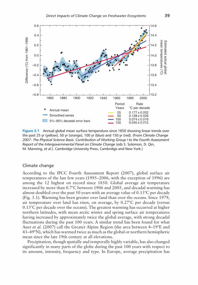
According to the IPCC Fourth Assessment Report (2007), global surface air temperatures of the last few years (1995–2006, with the exception of 1996) are among the 12 highest on record since 1850. Global average air temperature increased by more than 0.7°C between 1906 and 2005, and decadal warming has almost doubled over the past 50 years with an average value of 0.13°C per decade (Fig. 3.1). Warming has been greater over land than over the oceans. Since 1979, air temperature over land has risen, on average, by 0.27°C per decade (versus 0.13°C per decade over the oceans). The greatest warming has occurred at higher northern latitudes, with mean arctic winter and spring surface air temperatures having increased by approximately twice the global average, with strong decadal fluctuations during the past 100 years. A similar trend has been found for what Auer et al. (2007) call the Greater Alpine Region (the area between 4–19°E and 43–49°N), which has warmed twice as much as the global or northern hemispheric mean since the late 19th century at all elevations.

Precipitation, though spatially and temporally highly variable, has also changed significantly in many parts of the globe during the past 100 years with respect to its amount, intensity, frequency and type. In Europe, average precipitation has

Figure 3.1 Annual global mean surface temperature since 1850 showing linear trends over the past 25 yr (yellow), 50 yr (orange), 100 yr (blue) and 150 yr (red). (From Climate Change 2007: The Physical Science Basis. Contribution of Working Group I to the Fourth Assessment Report of the Intergovernmental Panel on Climate Change (eds S. Solomon, D. Qin, M. Manning, et al.). Cambridge University Press, Cambridge and New York.)

1880

Annual mean

PeriodYears25 0.177 ± 0.052

0.128 ± 0.0260.074 ± 0.0180.045 ± 0.012

50100150

Rate�C per decade

Smoothed series

5%–95% decadal error bars

1900 1920 1940 1960 1980 2000

14.6

14.4

14.2

Estim

ated actual globalm

ean temperatures (�C

)

14.0

13.8

13.6

13.4

13.2

0.6

0.4

0.2

0.0

Diff

eren

ce (

�C)

from

196

1–19

90

–0.2

–0.4

–0.6

–0.81860

9781405179133_4_003.indd 399781405179133_4_003.indd 39 7/9/2010 1:59:26 PM7/9/2010 1:59:26 PM

40 Ulrike Nickus et al.

increased in northern parts, while precipitation has decreased in the Mediterranean (IPCC 2007). These tendencies may be associated with changes in the North Atlantic Oscillation (NAO), a north–south dipole in sea-level pressure across the Atlantic (e.g. Hurrell et al. 2003), which has its strongest signature in winter. The prevalence of more positive winter NAO values from the 1970s to the 1990s reflects the enhanced westerly air flow across the North Atlantic, moving warm moist air over much of Europe in winter and resulting in wet conditions in Northern Europe and dry conditions in the south. However, topography may generate fine spatial scales in climate, and observed changes in air temperature or precipitation may thus differ from the average picture.

The IPCC Fourth Assessment Report (2007) notes that the increase in air temperature since the middle of the last century is very likely (i.e. >90% prob-ability) to be due to the increase in anthropogenic greenhouse gas concentrations. The observed changes can be accurately simulated only if climate models include greenhouse gas forcing (Fig. 3.2).

What can we expect for a future climate? General Circulation Models (GCMs) give a temperature increase of about 0.2°C per decade over the next two decades for a range of emission scenarios (IPCC 2007). Further warming will be caused by the continued emission of greenhouse gases at or above current rates. The projected changes in the climate system during this century are very likely to be

Models using only natural forcings

Models using both natural and anthropogenic forcings

Europe

Tem

pera

ture

ano

mal

y (°

C)

1.0

0.5

0.0

1900 1950

Year

2000

Figure 3.2 Temperature change relative to the 1901–50 mean for the period 1906–2005. The black line indicates observed values, the coloured bands give the modelled data covered by 90% of the recent model simulations. (Modified from Climate Change 2007: The Physical Science Basis. Contribution of Working Group I to the Fourth Assessment Report of the Intergovernmental Panel on Climate Change (eds S. Solomon, D. Qin, M. Manning, et al.). Cambridge University Press, Cambridge and New York.)

9781405179133_4_003.indd 409781405179133_4_003.indd 40 7/9/2010 1:59:26 PM7/9/2010 1:59:26 PM


larger than those observed during the 20th century. The best estimate of the global average surface warming, expressed as the temperature change from 1980–99 to 2090–99, is projected to range from 1.8°C for the low emissions scenario, B1, to 4.0°C for the high scenario, A1F1. Even for the case of a constant radiative forcing, if greenhouse gases and aerosols were kept constant at year 2000 levels, models give a temperature increase of a further 0.6°C by the end of the century.

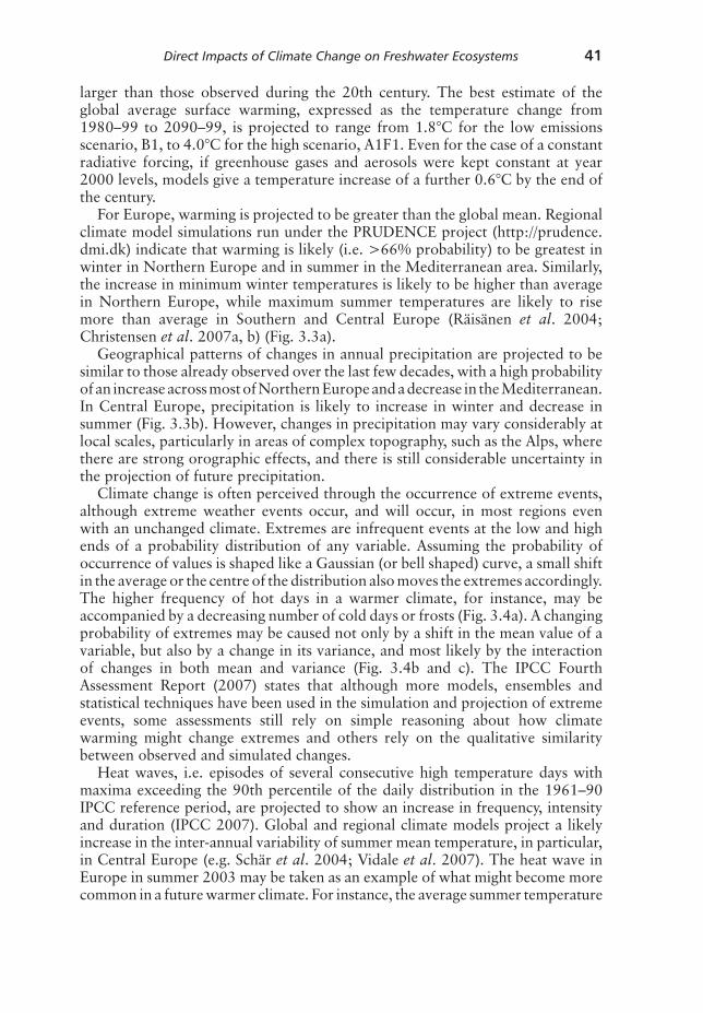
For Europe, warming is projected to be greater than the global mean. Regional climate model simulations run under the PRUDENCE project (http://prudence.dmi.dk) indicate that warming is likely (i.e. >66% probability) to be greatest in winter in Northern Europe and in summer in the Mediterranean area. Similarly, the increase in minimum winter temperatures is likely to be higher than average in Northern Europe, while maximum summer temperatures are likely to rise more than average in Southern and Central Europe (Räisänen et al. 2004; Christensen et al. 2007a, b) (Fig. 3.3a).

Geographical patterns of changes in annual precipitation are projected to be similar to those already observed over the last few decades, with a high probability of an increase across most of Northern Europe and a decrease in the Mediterranean. In Central Europe, precipitation is likely to increase in winter and decrease in summer (Fig. 3.3b). However, changes in precipitation may vary considerably at local scales, particularly in areas of complex topography, such as the Alps, where there are strong orographic effects, and there is still considerable uncertainty in the projection of future precipitation.

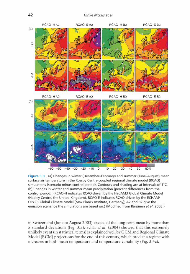
Climate change is often perceived through the occurrence of extreme events, although extreme weather events occur, and will occur, in most regions even with an unchanged climate. Extremes are infrequent events at the low and high ends of a probability distribution of any variable. Assuming the probability of occurrence of values is shaped like a Gaussian (or bell shaped) curve, a small shift in the average or the centre of the distribution also moves the extremes accordingly. The higher frequency of hot days in a warmer climate, for instance, may be accompanied by a decreasing number of cold days or frosts (Fig. 3.4a). A changing probability of extremes may be caused not only by a shift in the mean value of a variable, but also by a change in its variance, and most likely by the interaction of changes in both mean and variance (Fig. 3.4b and c). The IPCC Fourth Assessment Report (2007) states that although more models, ensembles and statistical techniques have been used in the simulation and projection of extreme events, some assessments still rely on simple reasoning about how climate warming might change extremes and others rely on the qualitative similarity between observed and simulated changes.

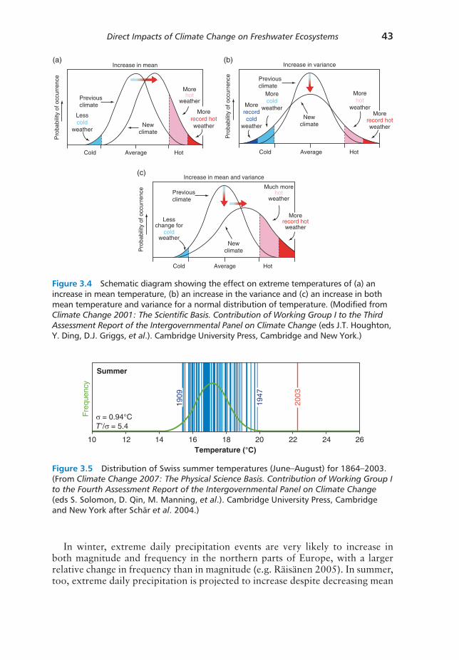
Heat waves, i.e. episodes of several consecutive high temperature days with maxima exceeding the 90th percentile of the daily distribution in the 1961–90 IPCC reference period, are projected to show an increase in frequency, intensity and duration (IPCC 2007). Global and regional climate models project a likely increase in the inter-annual variability of summer mean temperature, in particular, in Central Europe (e.g. Schär et al. 2004; Vidale et al. 2007). The heat wave in Europe in summer 2003 may be taken as an example of what might become more common in a future warmer climate. For instance, the average summer temperature

9781405179133_4_003.indd 419781405179133_4_003.indd 41 7/9/2010 1:59:26 PM7/9/2010 1:59:26 PM


in Switzerland (June to August 2003) exceeded the long-term mean by more than 5 standard deviations (Fig. 3.5). Schär et al. (2004) showed that this extremely unlikely event (in statistical terms) is explained well by GCM and Regional Climate Model (RCM) projections for the end of this century, which predict a regime with increases in both mean temperature and temperature variability (Fig. 3.4c).

Figure 3.3 (a) Changes in winter (December–February) and summer (June–August) mean surface air temperature in the Rossby Centre coupled regional climate model (RCAO) simulations (scenario minus control period). Contours and shading are at intervals of 1°C. (b) Changes in winter and summer mean precipitation (percent differences from the control period). (RCAO-H indicates RCAO driven by the HadAM3 Global Climate Model (Hadley Centre, the United Kingdom), RCAO-E indicates RCAO driven by the ECHAM/OPYC3 Global Climate Model (Max Planck Institute, Germany); A2 and B2 give the emission scenarios the simulations are based on.) (Modified from Räisänen et al. 2003.)

9781405179133_4_003.indd 429781405179133_4_003.indd 42 7/9/2010 1:59:26 PM7/9/2010 1:59:26 PM


Pro

babi

lity

of o

ccur

renc

e

Pro

babi

lity

of o

ccur

renc

e

Average

Increase in mean

Previousclimate

Previousclimate

Newclimate

Newclimate

Lesscold

weather

Morerecordcold

weather

Morecold

weather

Morehot

weatherMorehot

weatherMore

record hotweather

Morerecord hotweather

Increase in variance

Cold

(a) (b)

Hot AverageCold Hot

Pro

babi

lity

of o

ccur

renc

e

Previousclimate

Newclimate

Lesschange for

coldweather

Much morehot

weather

Morerecord hotweather

Increase in mean and variance(c)

AverageCold Hot

Figure 3.4 Schematic diagram showing the effect on extreme temperatures of (a) an increase in mean temperature, (b) an increase in the variance and (c) an increase in both mean temperature and variance for a normal distribution of temperature. (Modified from Climate Change 2001: The Scientific Basis. Contribution of Working Group I to the Third Assessment Report of the Intergovernmental Panel on Climate Change (eds J.T. Houghton, Y. Ding, D.J. Griggs, et al.). Cambridge University Press, Cambridge and New York.)

In winter, extreme daily precipitation events are very likely to increase in both magnitude and frequency in the northern parts of Europe, with a larger relative change in frequency than in magnitude (e.g. Räisänen 2005). In summer, too, extreme daily precipitation is projected to increase despite decreasing mean

10 12 14 16Temperature (°C)

Summer

2003

σ = 0.94°CT '/σ = 5.4

Fre

quen

cy

18 20 22 24 26

1909

1947

Figure 3.5 Distribution of Swiss summer temperatures (June–August) for 1864–2003. (From Climate Change 2007: The Physical Science Basis. Contribution of Working Group I to the Fourth Assessment Report of the Intergovernmental Panel on Climate Change (eds S. Solomon, D. Qin, M. Manning, et al.). Cambridge University Press, Cambridge and New York after Schär et al. 2004.)

9781405179133_4_003.indd 439781405179133_4_003.indd 43 7/9/2010 1:59:34 PM7/9/2010 1:59:34 PM


precipitation, but the expected magnitude of the change strongly depends on the climate model employed.

Future climate scenarios and Euro-limpacs

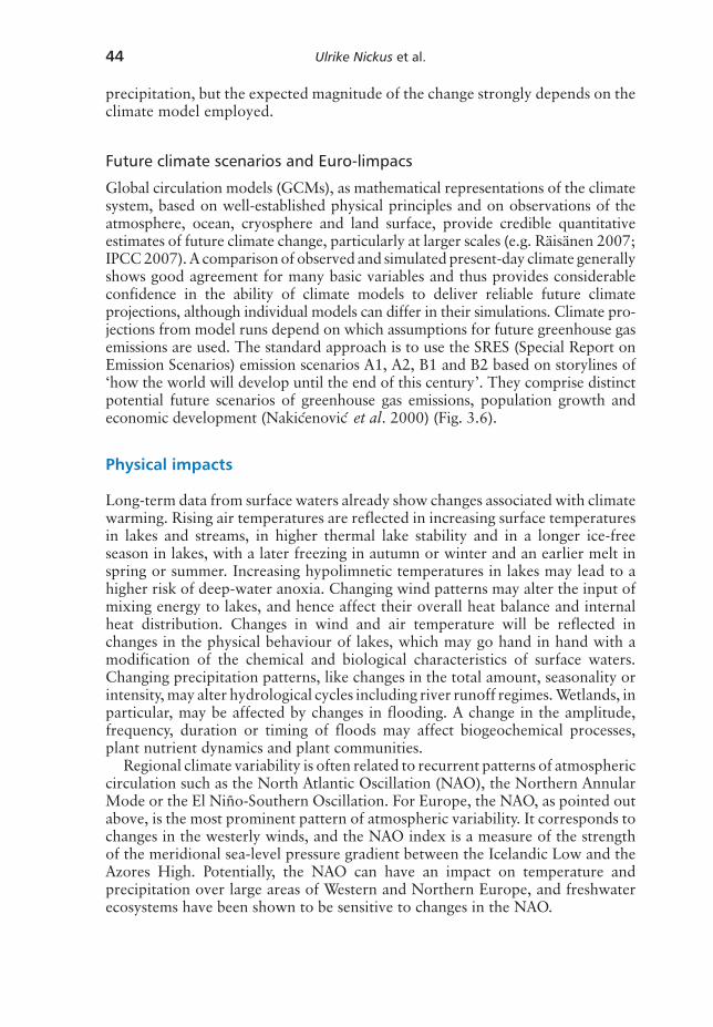
Global circulation models (GCMs), as mathematical representations of the climate system, based on well-established physical principles and on observations of the atmosphere, ocean, cryosphere and land surface, provide credible quantitative estimates of future climate change, particularly at larger scales (e.g. Räisänen 2007; IPCC 2007). A comparison of observed and simulated present-day climate generally shows good agreement for many basic variables and thus provides considerable confidence in the ability of climate models to deliver reliable future climate projections, although individual models can differ in their simulations. Climate pro-jections from model runs depend on which assumptions for future greenhouse gas emissions are used. The standard approach is to use the SRES (Special Report on Emission Scenarios) emission scenarios A1, A2, B1 and B2 based on storylines of ‘how the world will develop until the end of this century’. They comprise distinct potential future scenarios of greenhouse gas emissions, population growth and economic development (Nakicenovic et al. 2000) (Fig. 3.6).

Physical impacts

Long-term data from surface waters already show changes associated with climate warming. Rising air temperatures are reflected in increasing surface temperatures in lakes and streams, in higher thermal lake stability and in a longer ice-free season in lakes, with a later freezing in autumn or winter and an earlier melt in spring or summer. Increasing hypolimnetic temperatures in lakes may lead to a higher risk of deep-water anoxia. Changing wind patterns may alter the input of mixing energy to lakes, and hence affect their overall heat balance and internal heat distribution. Changes in wind and air temperature will be reflected in changes in the physical behaviour of lakes, which may go hand in hand with a modification of the chemical and biological characteristics of surface waters. Changing precipitation patterns, like changes in the total amount, seasonality or intensity, may alter hydrological cycles including river runoff regimes. Wetlands, in particular, may be affected by changes in flooding. A change in the amplitude, frequency, duration or timing of floods may affect biogeochemical processes, plant nutrient dynamics and plant communities.

Regional climate variability is often related to recurrent patterns of atmospheric circulation such as the North Atlantic Oscillation (NAO), the Northern Annular Mode or the El Niño-Southern Oscillation. For Europe, the NAO, as pointed out above, is the most prominent pattern of atmospheric variability. It corresponds to changes in the westerly winds, and the NAO index is a measure of the strength of the meridional sea-level pressure gradient between the Icelandic Low and the Azores High. Potentially, the NAO can have an impact on temperature and precipitation over large areas of Western and Northern Europe, and freshwater ecosystems have been shown to be sensitive to changes in the NAO.

9781405179133_4_003.indd 449781405179133_4_003.indd 44 7/9/2010 1:59:34 PM7/9/2010 1:59:34 PM


The Emission Scenario of the Special Report on Emission Scenarios (SRES)

A1. The A1 storyline and scenario family describes a future world of very rapid economic growth, global population that peaks in mid-century and declines thereafter and the rapid introduction of new and more efficient technologies. Major underlying themes are convergence among regions, capacity building and increased cultural and social interactions, with a substantial reduction in regional differences in per capita income. The A1 scenario family develops into three groups that describe alternative directions of technological change in the energy system. The three A1 groups are distinguished by their technological emphasis: fossil intensive (A1FI), non-fossil energy sources (A1T), or a balance across all sources (A1B) (where balanced is defined as not relying too heavily on one particular energy source, on the assumption that similar improvement rates apply to all energy supply and end-use technologies).

A2. The A2 storyline and scenario family describes a very heterogeneous world. The underlying theme is self- reliance and preservation of local identities. Fertility patterns across regions converge very slowly, which results in continuously increasing population. Economic development is primarily regionally oriented and per capita economic growth and technological change more fragmented and slower than other storylines.

B1. The B1 storyline and scenario family describes a convergent world with the same global population that peaks in mid-century and declines thereafter, as in the A1 storyline, but with rapid change in economic structures toward a service and information economy, with reductions in material intensity and the introduction of clean and resource-efficient technologies. The emphasis is on global solutions to economic, social and environmental sustainability, including improved equity, but without additional climate initiatives.

B2. The B2 storyline and scenario family describes a world in which the emphasis is on local solutions to economic, social and environmental sustainability. It is a world with continuously increasing global population, at a rate lower than A2, intermediate levels of economic development, and less rapid and more diverse technological change than in the A1 and B1 storylines. While the scenario is also oriented towards environmental protection and social equity, it focuses on local and regional levels.

An illustrative scenario was chosen for each of the six scenario groups A1B, A1FI, A1T, A2, B1 and B2. All should be considered equally sound.

The SRES scenarios do not include additional climate initiatives, which means that no scenarios are included that explicitly assume implementation of the United Nations Framework Convention on Climate Change or the emission targets of the Kyoto protocol.

Figure 3.6 Description of the SRES emission scenarios (Climate Change 2007: The Physical Science Basis. Contribution of Working Group I to the Fourth Assessment Report of the Intergovernmental Panel on Climate Change (eds S. Solomon, D. Qin, M. Manning, et al.). Cambridge University Press, Cambridge and New York.)

There is now much evidence for these observed trends and potential future changes to freshwaters as a result of climate change. Here, we present a series of examples and case studies based on the analysis of long-term data series, field experiments and physical modelling.

Thermal regimes of lakes and streams

The thermal regime of water bodies is mainly determined by the local weather. The net heat exchange across the air–water interface is given by the sum of energy fluxes related to radiation, latent and sensible heat (Edinger et al. 1968; Imboden & Wüest 1995). A shift in climate variables such as air temperature, radiation, cloud cover, wind or humidity will influence these heat fluxes and thus alter the heat balance of lakes and rivers. Model studies predict that lake temperatures, especially in the epilimnion, will increase with increasing air temperature, so that temperature profiles, thermal stability and mixing patterns are expected to change as a result of climate change (e.g. Hondzo & Stefan 1993; Stefan et al. 1998).

9781405179133_4_003.indd 459781405179133_4_003.indd 45 7/9/2010 1:59:34 PM7/9/2010 1:59:34 PM


Analyses of long-term data series demonstrate that such a change has already occurred in recent decades. One of the first studies on increasing water temperatures was on boreal soft water lakes in the Experimental Lakes Area of north-western Ontario (Canada) by Schindler et al. (1990). The authors showed that these lakes experienced an increase in water temperature of c. 2°C between 1969 and 1988 and that water renewal rates decreased as a result of higher-than-normal evaporation and lower-than-average precipitation. At Lake Tahoe in the south-west USA, volume-weighted lake temperature increased by about 0.15°C per decade between 1970 and 2002 with a concomitant increase in lake thermal stability (Coats et al. 2006). At Lake Baikal, the world’s largest lake, with a maximum depth of 1600 m, surface waters have warmed at a rate of 0.2°C per decade over the past 60 years (Hampton et al. 2008). Lake Baikal was expected to be rather resistant to climate change due to its enormous volume, but even here, increasing water temperatures and a longer ice-free season are having major implications for nutrient cycling and food-web structure. In Lake Constance, a warm monomictic lake in Central Europe, the mean annual water temperature has increased by 0.17°C per decade since the 1960s (Straile et al. 2003). This warming is strongly related to increasing winter air temperatures and has affected the duration and extent of winter lake mixing, the heat content of the lake and the vertical distribution of oxygen and nutrients. Reduced winter cooling favours the persistence of small temperature gradients and may result in an incomplete mixing of the lake.

Fluctuations in lake surface water temperatures are transported downwards by vertical mixing, and can reach the deep waters when the thermal stratification is weak. In particular, the hypolimnetic temperatures of deep lakes, which are determined by winter meteorological conditions and the amount of heat reaching deep-water layers before the onset of thermal stratification may act as a ‘climate memory’. Increasing air temperatures may thus lead to a progressive rise in deep-water temperatures, as found, for instance, by Ambrosetti & Barbanti (1999) for lakes in Northern Italy.

Dokulil et al. (2006) reported a coherent warming in the hypolimnia of 12 deep lakes across Europe. Annual mean hypolimnetic temperatures increased by about 0.1°C–0.2°C per decade during the past 20–50 years, despite differences between lakes and years. Hypolimnetic temperatures in most lakes tended to reflect fluctuations in the North Atlantic Oscillation (NAO) with the winter- to-spring NAO index explaining 20%–60% of the inter-annual variability in deep-water temperatures. In particular, winter-to-spring periods with a high positive NAO index were associated with high hypolimnetic water temperatures, when warmer-than-average surface water was transported downwards during spring overturn. However, the strength and persistence of the climate signal with time and depth are determined by the lakes’ geographical location, landscape topo graphy, mixing conditions and lake morphometry.

The thermal regime of Lake ZurichLake Zurich, a 136-m deep peri-alpine lake in Switzerland, has one of the longest temperature data series in Europe with water temperature profiles measured at approximately monthly intervals since the 1940s (Livingstone 1993). This lake

9781405179133_4_003.indd 469781405179133_4_003.indd 46 7/9/2010 1:59:34 PM7/9/2010 1:59:34 PM


provides a good example of the response of deep temperate lakes to long-term changes in air temperature. The lake has undergone long-term warming at all depths. However, the temperature increase has been more rapid in the surface layers than in the deep-water layers, resulting in increased thermal stability in all seasons and in an extended period of summer stratification by about 2–3 weeks from the 1950s to the 1990s (Livingstone 2003).

In winter (December–February), highly significant increasing trends in water temperature have occurred at all depths (Mann-Kendall test (MK), p < 0.001), but the highest long-term winter warming rates (∼0.15°C per decade) are found in the uppermost part of the water column (0–10 m) (Fig. 3.7a). From 10 to 80 m, long-term warming rates decrease with increasing depth, but from 80 m to the lake bottom, no further change occurs; warming rates remain approximately constant at about 0.06°C per decade. In summer, the highest rate of long-term warming (0.42°C per decade; MK, p < 0.01) has occurred at 10-m depth (Fig. 3.7b), while at the lake surface, the temperature increase since the 1950s has been comparatively low (∼0.07°C per decade; MK, p < 0.01). Surface water temperatures approximately reflect the behaviour of the regional summer air temperature, and reveal a period of rapid cooling from 1945 to 1970 (−1.0°C per decade) followed by strong warming from 1970 to 2006 (0.5°C per decade).

7.0Winter

(a) (b)

(c)

T (

°C)

T (

°C)

10 m (0.15°C/decade)

100 m (0.06°C/decade)

17.0

16.0

15.0

14.0

13.0

12.0

11.0

10.01950 1960 1970

Summer

10 m (0.42°C/decade)

1980 1990 2000

1950 1960 1970 1980 1990 2000

6.0

5.0

4.0

Summer

100 m (0.03°C / decade)

1950 1960 1970 1980 1990 2000

6.0

5.0

4.0

Figure 3.7 Warming trends in Lake Zurich (Switzerland) showing linear regression lines and their gradients: (a) at 10 and 100 m depth in winter (December, January, February), (b) at 10 m depth in summer (June, July, August) and (c) at 100 m depth in summer.

9781405179133_4_003.indd 479781405179133_4_003.indd 47 7/9/2010 1:59:34 PM7/9/2010 1:59:34 PM


In the hypolimnion (i.e. below 20 m), summer temperatures show a low long-term warming trend of 0.03°C–0.06°C per decade, which is, however, not statistically significant even at the p < 0.1 level (Fig. 3.7c).

As in most deep, temperate-zone lakes, temperatures in the uppermost 10–20 m of Lake Zurich are influenced directly by weather in all seasons, whilst temperatures in the deeper water respond most strongly to weather in winter and spring. Physically, Lake Zurich appears to be quite sensitive to climate variability since it can behave either as a dimictic, monomictic or oligomictic lake, mixing twice or once per year or not mixing at all, respectively. Over the past few decades, the frequency of dimixis (after ice melt and in autumn) has decreased, while the frequency of years with incomplete mixing has increased as winters have become warmer (Livingstone 1997; Peeters et al. 2002).

In Central Europe, the summer of 2003 was exceptionally hot, with air temperatures similar to those predicted for an average summer during the late 21st century (Schär et al. 2004). During that summer, Lake Zurich experienced the highest epilimnetic temperatures ever recorded, exceeding the long-term mean (1856–2002) by almost three standard deviations (Fig. 3.8). By contrast, hypolimnetic temperatures were slightly lower than average. The resulting high thermal stability of the water column resulted in hypolimnetic oxygen depletion exceeding its long-term mean by more than seven standard deviations. The potential ecological consequences of this, such as the release of phosphorus from the sediments, possibly ultimately resulting in an increase in the intensity of algal blooms, may thus counteract management and restoration efforts undertaken in the past to mitigate anthropogenic eutrophication.

Figure 3.8 Standardized values of water temperature, Schmidt stability (the quantity of work required to mix a lake to a uniform vertical density with no addition or substraction of heat) and hypolimnetic oxygen depletion in Lake Zurich (Switzerland). Data are expressed as standard deviations from the long-term mean (μ) of 1956–2002. The summer 2003 values are shown in red. (Modified from Jankowski et al. 2006. Reproduced with permission of the American Society of Limnology and Oceanography.)

86

μ = 4.3 g m–3

μ = 8780 J m–2

μ = 11.2°C

μ = 4.8°C

μ = 16.0°C

42Number of standard deviations

Hypolimneticoxygen depletion (HOD)

Schmidtstability (S )

Temperaturedifference (Tem–Th)

Epi/metalimnetictemperature (Tem)

Hypolimnetictemperature (Th)

0–2–4

9781405179133_4_003.indd 489781405179133_4_003.indd 48 7/9/2010 1:59:34 PM7/9/2010 1:59:34 PM


The whole-lake mixing experiment THERMOSIncreasing average wind speed is expected to raise the input of mixing energy to lakes. This scenario, i.e. increasing geostrophic winds due to a northward shift in cyclone activity and a higher air surface temperature by the end of this century, is projected for the north of Europe.

A whole-lake manipulation experiment in the small humic Lake Hälsjärvi in Southern Finland simulated the increasing input of mixing energy and its impact on the stratification cycle and heat balance of the lake (M. Forsius unpublished data, 2009). A submerged propeller caused the thermocline to deepen by about 2 m during two summer periods in 2005 and 2006 compared with the reference years and the nearby reference lake Valkea-Kotinen (Fig. 3.9).

The observed deepening of the thermocline in Lake Hälsjärvi corresponds to modelled impacts on the lake thermal regime under the A2 SRES emission scenario. Simulations with the MyLake model (Multi-year Lake simulated model; Saloranta & Andersen 2007) simulated an increase in the mean heat content of about 9.5 MJ m−3, which is equivalent to an increase in the average water temperature by 2.3°C in summer and early autumn compared with the reference period 1961–90 (Saloranta et al. 2009). The increased mean heat content in the manipulation experiment was about 11 MJ m−3 (equivalent to a 2.6°C increase in the water mass temperature) in the same period, indicating that the lake manipulation experiment well represented the mean simulated future increase in heat content in the summer and autumn. A consequence of the lowered

Figure 3.9 Interpolated seasonal development of temperature in the experimental Lake Halsjärvi (top) and the reference Lake Valkea-Kotinen (bottom) in the reference year (2004) and in the two experimental years 2005 and 2006 (M. Forsius unpublished data, 2009).

0

1

2

3

4

5Apr May Jun Jul Aug Sep Oct Nov

0

1

2

3

4


0

1

2

3

4

5

0

2

4

6

8

10

12

14

16

18

20

22

24

26

28

Apr May Jun Jul Aug Sep Oct Nov

0

1

2

3

4

5

6Apr May Jun Jul Aug Sep

Dep

th(m

)D

epth

(m)

Oct Nov

0

1

2

3

4

5


0

1

2

3

4

5


Hälsjärvi 2004 temperature (�C)

Valkea-Kotinen 2004 temperature (�C) Valkea-Kotinen 2005 temperature (�C) Valkea-Kotinen 2006 temperature (°C)

Hälsjärvi 2005 temperature (�C) Hälsjärvi 2006 temperature (�C)

9781405179133_4_003.indd 499781405179133_4_003.indd 49 7/9/2010 1:59:35 PM7/9/2010 1:59:35 PM


thermocline in Lake Hälsjärvi was a change in the oxygen stratification during the summers of 2005 and 2006. While the minimum oxygenated layer was only 1 m deep in 2004, mixing increased its depth to 3.5 m in the experimental years 2005 and 2006. The manipulation experiment also affected nutrient levels in Lake Hälsjärvi, causing a statistically significant decline in total nitrogen and ammonia (M. Forsius unpublished data, 2009). Changes in lake temperature, oxygen distribution and nutrient levels in the lake also affected the phytoplankton (L. Arvola unpublished data, 2009). The biomass of diatoms and non-flagellated green algae increased as well as the rate of change of the phytoplankton community, while the zooplankton and fish communities remained steady.

Another whole-lake manipulation experiment conducted in the deeper, oligotrophic clear-water lake Breisjon in Norway increased the thermocline depth (from 6 to 20 m) and the mean temperature at the time of maximum heat content (from 10.7°C to 17.4°C) and delayed freezing by about 20 days (Lydersen et al. 2008). During the experimental manipulation, only minor changes in water chemistry, nutrients and water transparency occurred, but planktonic chlorophytes and diatoms decreased, mixotrophic dinoflagellates increased and periphyton biomass increased. The manipulation did not affect zooplankton biodiversity and did not affect fish populations (i.e. size, condition factor or population density of perch and brown trout).

Water temperature in Swiss rivers and streamsRivers and streams have also warmed during the past few decades, and stream water temperatures are projected to increase further in a future warmer climate (e.g. Stefan & Sinokrot 1993; Webb 1996). Many studies have used linear regression models of stream temperature versus air temperature to explain the variance in water temperature (cf. Mohensi & Stefan 1999 and references therein). However, in addition to meteorological variables, the energy budget and thermal capacity of rivers and streams may be heavily affected by human activities such as the increased input of heated cooling waters from power plants.

Within Euro-limpacs, water temperatures in rivers and streams across Switzerland, covering an altitudinal range of more than 4000 m, were studied by Hari et al. (2006). The study showed parallel warming at all altitudes, reflecting the changes in regional air temperature during the past 40 years (Fig. 3.10). Regional coherence (i.e. spatial correlation between time series within a region) was high for rivers and streams on the Swiss Plateau and in the foothills of the Alps, but decreased with increasing altitude. In catchments containing glaciers or hydroelectric power stations, the warming was strongly reduced, presumably owing to the influence of inflowing melt water from glaciers and deep-water from reservoirs.

The effects of warming on populations of cold-water fish, such as brown trout, are expected to be deleterious at the warmer boundaries of their habitat and positive at the cooler boundaries. On the Swiss Plateau, brown trout populations inhabit the upper limit of their range of temperature tolerance. There, a potential upward migration of fish due to increasing water temperatures is often impeded by natural and artificial physical barriers, and a climatically driven upward habitat shift increases the likelihood of a population decrease. Hari et al. (2006)

9781405179133_4_003.indd 509781405179133_4_003.indd 50 7/9/2010 1:59:35 PM7/9/2010 1:59:35 PM


11

10

9

8

71965 1970 1975

Tem

pera

ture

(°C

)

1980 1985 1990 1995 2000

Figure 3.10 Mean water temperature of rivers and streams measured at 25 stations in Switzerland (black line) and mean air temperature at Basle and Zurich (thin blue curve). The data illustrated are annual running means. (Modified from Hari et al. 2006.)

found that such a climate-related decrease in brown trout population had already occurred in alpine rivers and streams in Switzerland, and was accelerated by an increasing incidence of temperature-dependent Proliferative Kidney Disease.

Ice-cover

The seasonal ice-cover of lakes and rivers plays an important role in freshwater systems, and changes in the thickness and duration of the ice layer are of ecological importance and have consequences for human activities. According to IPCC (2007), freeze-up is defined conceptually as the time at which a continuous and immobile ice-cover forms, while break-up is generally the time when open water becomes extensive in a lake or when the ice-cover starts to move downstream in a river. Major variables affecting duration and thickness of lake and river ice are air temperature, wind, snow depth, heat content of the water body and rate and temperature of potential inflows. Dates of freeze-up and ice break-up have proved to be good indicators of climate variability at local to regional scales, and as a response to large-scale atmospheric forcing (e.g. Walsh 1995; Livingstone 1999, 2000; Yoo & D’Odorico 2002; Blenckner et al. 2004). Thus, as climate changes, and air temperatures, particularly in the winter, tend to increase, these shifts should be reflected in ice-cover. Moreover, several authors have used the correlation of ice-cover dates and air temperature to translate shifts in freeze-up and break-up into estimated changes in air temperature (e.g. Palecki & Barry 1986; Robertson et al. 1992; Assel & Robertson 1995; Magnuson et al. 2000). A typical value for lakes at mid-latitudes is a 4–5-day shift in mean freeze-up or break-up dates for each degree Celsius change in mean autumn or spring temperatures. Relationships tend to be stronger for freezing dates and in colder climates (Walsh 1995).

Generally, time series of ice phenology data from lakes and rivers in Eurasia and North America provide evidence of later freezing and earlier break-up of the seasonal ice-cover. For instance, long-term ice-cover records of 26 selected lakes and rivers in the northern hemisphere revealed that from 1884 to 1995, the average

9781405179133_4_003.indd 519781405179133_4_003.indd 51 7/9/2010 1:59:35 PM7/9/2010 1:59:35 PM


date of freezing and break-up, both advanced by about 6 days per 100 years (Magnuson et al. 2000). This prolongation of the ice-free season translates to a 1.2°C increase in air temperature per 100 years. Inter-annual variability in the ice phenology data from the selected rivers and lakes has increased since the 1950s. At Lake Baikal, the ice-free season has lengthened by about 16 days per 100 years, with a more consistent trend towards later freezing despite variability from decade to decade. The trend towards earlier break-up occurred mainly before 1920 (Livingstone 1999; Magnuson et al. 2000; Todd & Mackay 2003) and reflects the close relationship of melting to the April mean air temperature, which has shown no trend since the 1920s, in contrast to other months of the winter. In Canada, most lakes have experienced earlier break-up and a longer ice-free season during the past decades (e.g. Futter 2003; Duguay et al. 2006). The trends in lake ice-cover provide further evidence of a spring warming that has been observed over North America since the second half of the 20th century. Ice phenology data from Lake Mendota (Wisconsin, the United States), the lake with the longest uninterrupted ice record in North America, dating back to 1855, showed three climatic periods with relatively stable ice conditions between 1890 and 1979 but decreasing trends in ice-cover duration before and after this period due to increasing winter/early spring air temperatures (Robertson et al. 1992).

Long series of lake ice data are available from Fennoscandia. Korhonen (2006) analysed freezing and break-up records of almost 90 lakes in Finland dating back to the early 19th century and ice thickness records of about 30 lakes dating back to the 1910s. There were significant changes with earlier ice break-up, except for the very north of Finland, and later freezing, resulting in shorter ice duration. Palecki & Barry (1986) conducted a statistical study of the relationship between ice phenology data and air temperature for Finnish lakes, and found that the same change in freeze-up date indicated a larger shift in autumn air temperature in the north of Finland than in Southern Finland. Ice phenology dates revealed a strong dependence on latitude, and the maritime influence of the Baltic Sea caused a northward deflection of average freezing and melting date isolines near the coast. A similar dependence of ice phenology on latitude was described by Blenckner et al. (2004) for 50 lakes in Fennoscandia. The prevalence of zonal or meridional winds in autumn and spring, expressed by regional circulation indices, was used to explain the temporal and regional variability of freeze-up and break-up dates.

An analysis of 54 Swedish lakes (Weyhenmeyer et al. 2005) confirmed the existence of trends in the timing of melting during the IPCC reference period (1961–90), but also showed that these trends were dependent on latitude. Trends towards earlier melting were substantially greater in warmer, southern Sweden than in the colder, northern regions. The non-linear dependence of break-up dates on latitude can be described in terms of an arc cosine function of lake-specific annual mean air temperature for 196 lakes across Sweden (1961–2002) (Weyhenmeyer et al. 2004). Thus, an increase in air temperature is expected to have greater impacts on the melting date in warmer southern Sweden compared with the colder north with mean annual air temperatures of −2°C to 2°C. The authors showed that the average temperature increase of 0.8°C from 1991 to 2002 across Sweden (compared with the reference period 1961–90) caused ice

9781405179133_4_003.indd 529781405179133_4_003.indd 52 7/9/2010 1:59:35 PM7/9/2010 1:59:35 PM


break-up to occur about 17 days earlier in the south of Sweden, i.e. south of 60°N, but only 4 days earlier in the northern part of the country.

An altitudinal gradient of ice phenology was studied in the Tatra Mountains of Poland and Slovakia (Šporka et al. 2006). Mini-thermistors with data loggers measured surface water temperatures in 19 morphologically different lakes, which covered an elevation range of almost 600 m (1580–2157 m a.s.l.). For practical reasons, freezing date was defined as the calendar date on which the measured lake surface water temperature decreased to 0°C, and the date on which it increased above 0°C again, represented melting date. Freeze-up dates spanned a period of 52 days, but exhibited no detectable dependence on altitude. Break-up dates, occurring between beginning of May and end of June, however, depended strongly on altitude. The average gradient in the timing of melting was about 9 days per 100 m and explained more than 60% of the variability. Ice-cover duration varied from 136 to 232 days and exhibited a significant linear dependence on altitude, at a rate of about 10 days per 100 m. In contrast to ice break-up, which depends strongly on altitude (as a proxy for air temperature), freezing appears to be governed not only by air temperature, but to a considerable extent by local factors like lake morphometry, exposure to radiation and wind, or inflows, which influence lake surface water temperature in autumn and early winter.

Chemical impacts

Climate not only has an impact on the physical characteristics of surface waters, but also is a master variable for ecologically important chemical processes. Here, we discuss two examples of how climate may directly or indirectly affect surface water chemistry, first with respect to changes in concentrations of dissolved organic carbon (DOC) and secondly related to increases in the release of major ions and heavy metals from active rock glaciers in high mountain regions.

Dissolved organic carbon in surface waters

DOC is an important constituent of many natural waters. It is generated by the partial decomposition of organic matter and may be stored in soils for varying lengths of time before transport to surface waters. The humic substances generated by organic matter decomposition impart a characteristic brown colour to the water due to the absorption of visible light by these compounds. DOC thus influences light penetration into surface waters, as well as their acidity, nutrient availability, metal transport and toxicity. During the past two decades, rising DOC concentrations have been observed across much of the British Isles (Fig. 3.11), large areas of Fennoscandia, parts of Central Europe, and northeastern North America (e.g. Freeman et al. 2001; Evans et al. 2005, 2006; Vuorenmaa et al. 2006; Monteith et al. 2007). When first observed, these increases were widely interpreted as evidence of climate-change impacts on terrestrial carbon stores due to rising temperatures and the increasing frequency and severity of summer droughts (e.g. Freeman et al. 2001; Hejzlar et al. 2003; Worrall et al. 2004). Increasing precipitation could also lead to increasing DOC concentrations, first

9781405179133_4_003.indd 539781405179133_4_003.indd 53 7/9/2010 1:59:35 PM7/9/2010 1:59:35 PM


by increasing the proportion of DOC-rich water derived from the upper organic horizons of mineral soils and secondly by reducing water residence time, and hence DOC removal, in lakes (Hongve et al. 2004). Rising levels of atmospheric CO2, influencing plant growth and litter quality were also proposed to explain increased rates of DOC production (Freeman et al. 2004).

Erlandsson et al. (2008) showed that for the 35-year period (1970–2004), most of the inter-annual variability of concentrations of dissolved organic matter (OM) in 28 large Scandinavian river catchments were explained by discharge and concentrations of sulphate, with discharge being the more important driver. Despite the heterogeneity of the catchments with regards to climate, size and land use, there was a high degree of synchroneity in chemical oxygen demand (COD), a common proxy for OM, across the entire region. Multiple regression models with discharge and sulphate concentration explained up to 78% of the annual variability in COD, while two other candidate drivers, air temperature and chloride concentration in river water, added little explanatory value (Fig. 3.12).

0.8

0.6

0.4

0.2

0.0

–0.2Temp QCI

r2 (a

djus

ted)

All varSO4Q+SO4

Figure 3.12 The variance in OM explained by the different potential drivers. Box-plot (10th, 25th, 50th, 75th, and 90th percentiles marked) of the r2-values for COD, modelled with linear regression for 28 rivers, using temperature, [Cl−], [SO4

2−] and flow as explanatory variables. Combinations of these parameters were modelled using multiple linear regression. (Modified from Erlandsson et al. 2008.)

Figure 3.11 Median DOC concentration (mg l−1) of surface waters in the UK Acid Water Monitoring Network, 1988–2007. (a) Lakes. (b) Streams. Bars show the 25th and 75th percentile concentrations at each sampling interval.

0123456789

(a) (b)

1988

mg

l–1

mg

l–1

1990

1992

1994

1996

1998

2000

2002

2004

2006

2008

0123456789

1988

1990

1992

1994

1996

1998

2000

2002

2004

2006

2008

9781405179133_4_003.indd 549781405179133_4_003.indd 54 7/9/2010 1:59:36 PM7/9/2010 1:59:36 PM


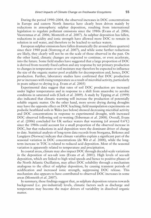
During the period 1990–2004, the observed increases in DOC concentrations in Europe and eastern North America have clearly been driven mainly by reductions in atmospheric sulphur deposition, resulting from international legislation to regulate pollutant emissions since the 1980s (Evans et al. 2006; Vuorenmaa et al. 2006; Monteith et al. 2007). As sulphur deposition has fallen, reductions in acidity and ionic strength have allowed more DOC to remain in solution in soil water, and therefore to be leached to surface waters.

European sulphur emissions have fallen dramatically (by around three quarters) since their 1980 peak (Vestreng et al. 2007), and while some further reductions are likely, they clearly will not be on the scale of those observed in the past. On the other hand, climatic changes are expected to continue, or even accelerate, into the future. Some field studies have suggested that a large proportion of DOC is derived from recently fixed carbon and any response by net primary production to changes in temperature or soil moisture may therefore be expected to influence the size of the organic matter pool available for decomposition and, hence, DOC production. Further, laboratory studies have confirmed that DOC production per se increases with rising temperature as a result of microbial activity, particularly in peats subject to drying (e.g. Evans et al. 2005)

Experimental data suggest that rates of soil DOC production are increased under higher temperatures and in response to a shift from anaerobic to aerobic conditions in saturated soils (Clark et al. 2009). A study by Tipping et al. (1999) also indicated that climatic warming will increase the production of potentially soluble organic matter. On the other hand, more severe drying during droughts may have the opposite effect on DOC leaching; field manipulation experiments on podsolic heathland soils in Wales (see below) showed decreasing microbial activity and DOC concentrations in response to experimental drought, with increased DOC observed following soil re-wetting (Toberman et al. 2008). Overall, Evans et al. (2006) concluded for UK surface waters that warming (of around 0.6°C) since the 1980s could account for a small proportion of the observed increase in DOC, but that reductions in acid deposition were the dominant driver of change to date. Statistical analysis of long-term data records from Storgama, Birkenes and Langtjern (Norway) indicate that climate variables explain a significant part of the seasonal variation in DOC concentrations (de Wit et al. 2008), while the long-term increase in TOC is related to reduced acid deposition. Most of the seasonal variation is apparently related to temperature and precipitation.

In coastal areas, climate may also impact DOC through decadal-scale variations in the deposition of sea-salt ions (Evans et al. 2001). High levels of sea-salt deposition, which are linked to high wind speeds and hence to positive phases of the North Atlantic Oscillation, may affect DOC solubility through a mechanism analogous to the effect of sulphur deposition, by causing transient periods of acidification and increased ionic strength, suppressing DOC release. This mechanism also appears to have contributed to observed DOC increases in some areas (Monteith et al. 2007).

In summary, these findings suggest that, as sulphate deposition returns towards background (i.e. pre-industrial) levels, climatic factors such as discharge and temperature may become the major drivers of variability in dissolved organic matter.

9781405179133_4_003.indd 559781405179133_4_003.indd 55 7/9/2010 1:59:36 PM7/9/2010 1:59:36 PM


The effect of soil frost and snow cover on DOC in surface waters – a manipulation experiment in northern SwedenSnow cover in northern regions provides a major fraction of the annual water budget, and it plays a fundamental role in regulating the winter biogeochemistry of soils in northern forests (Groffman et al. 2001). Snow cover limits or even prevents the development of soil frost. Changes in the timing, extent and duration of the snow cover, as projected under a future warmer climate, may result in an increased number of freeze–thaw events, or longer snow-free periods during winter (Stieglitz et al. 2003; Mellander et al. 2007). As DOC in some streams is strongly controlled by soil solution chemistry in the riparian zone, changes here could alter both quantity and bioavailability of DOC exported to the adjacent streams during the spring flood – up to half of the annual runoff and DOC flux may occur during snow melt in small streams and rivers in northern Sweden (Ågren et al. 2007). Moreover, many boreal surface waters experience a pH decline of one to two pH units during snow melt, driven primarily by a transient increase in DOC export from the terrestrial systems (Buffam et al. 2007).

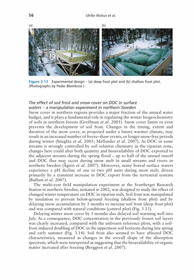
The multi-year field manipulation experiment at the Svartberget Research Station in northern Sweden, initiated in 2002, was designed to study the effect of changed winter temperature on DOC in riparian soils. Soil frost was manipulated by insulation to prevent below-ground freezing (shallow frost plot) and by delaying snow accumulation by 3 months to increase soil frost (deep frost plot) and was compared with natural conditions (control plot) (Fig. 3.13).

Delaying winter snow cover by 3 months also delayed soil warming well into July. As a consequence, DOC concentration in the previously frozen soil layers was clearly increased, compared with the unfrozen reference plots, with a soil-frost-induced doubling of DOC in the uppermost soil horizons during late spring and early summer (Fig. 3.14). Soil frost also seemed to have affected DOC characteristics, measured as changes in the overall shape of the absorption spectrum, which were interpreted as suggesting that the bioavailability of organic matter increased after freezing (Berggren et al. 2007).

(a) (b)

Figure 3.13 Experimental design – (a) deep frost plot and (b) shallow frost plot. (Photographs by Peder Blomkvist.)

9781405179133_4_003.indd 569781405179133_4_003.indd 56 7/9/2010 1:59:36 PM7/9/2010 1:59:36 PM


The quality and quantity of DOC in the soil frost experiment during the winter seemed to be controlled by lysis of cell structures and by limiting the soil microbial activity. While freeze-out processes are believed mainly to control the concentration of DOC in soil solution below the expanding ice during freezing, lysis of cells may release highly bioavailable organic compounds of low molecular weight and low C/N ratio (Stepanauskas et al. 2000). Temperatures below freezing are unfavourable for heterotrophic microbial activity. This may result in undecomposed organic material of high substrate quality that subsequently will be decomposed during unfrozen conditions. As a consequence, the soil frost experiment has shown that the thermal conditions in the soil ecosystem influence the soil organic matter decomposition rate and CO2 production (Öquist & Laudon 2008).

The effect of summer droughts on soil solution DOC – the Clocaenog experiment (the United Kingdom)In many areas of Europe, climate change is projected to lead to increased frequency and severity of summer droughts. At Clocaenog, a heathland site in North Wales, the United Kingdom, repeated summer droughts have been experimentally induced each year since 1999, initially as part of the CLIMOOR (Climate Driven Changes in the Functioning of Heath and Moorland Ecosystems) and VULCAN (Vulnerability assessment of shrubland ecosystems in Europe under climatic changes) projects. A retractable transparent roof system was used to reduce summer rainfall by around 60%, for a set of replicated 20 m2 plots (Beier et al. 2004).

Droughts were found to reduce rates of soil respiration, as biological activity became moisture limited. Measurements of soil solution DOC (Fig. 3.15) suggest that DOC production is similarly affected; in the control plots, DOC concentrations consistently increase in summer, but in the drought plots concentrations can fall

–10

0 50 100

DOC (mg l–1)

No soil frostD

epth

(cm

)

150 200

April 1

May 1

June 1

July 1

–30

–50

–70

–90

30 cm soil frost

DOC (mg l–1)

Dep

th (

cm)

–10

0 50 100 150 200

–30

–50

–70

–90

April 1

May 1

June 1

July 1

Figure 3.14 Concentration profiles of DOC in the soil during winter, spring and early summer (April–July) at five soil depths in plots without and with deep soil frost.

9781405179133_4_003.indd 579781405179133_4_003.indd 57 7/9/2010 1:59:39 PM7/9/2010 1:59:39 PM


to much lower levels. In some years (e.g. in 2004), it appears that this drought-induced reduction was followed by increased concentrations on re- wetting, although this was not observed in all years. Similar patterns of reduced DOC concentrations during droughts, and raised concentrations on re-wetting, have been noted in several previous studies of peatland soil solutions and surface waters (e.g. Watts et al. 2001; Clark et al. 2005). Other work undertaken at the Clocaenog site suggests that reduced DOC losses in summer are linked to decreased activity of the phenol oxidase enzyme, which has an important role in litter decomposition and DOC production (Toberman et al. 2008). In the mineral soil solutions at Clocaenog, on the other hand, changes to the seasonal cycle are less evident; instead, there is some indication that repeated droughts are leading to progressive, year-round DOC increases (Fig. 3.15).

Figure 3.15 DOC concentrations over 4 years of experimentally induced summer drought on a heathland at Clocaenog, North Wales, the United Kingdom. Shaded areas indicate experimental drought periods.

Organic horizon

Mineral horizon

Jan

2003

90

80

70

60

50

40

30

20

10

0

DO

C (

mg

l–1)

35

30

25

20

15

5

10

0

DO

C (

mg

l–1)

Jul 2

003

Jan

2004

Jul 2

004

Jan

2005

Jul 2

005

Jan

2006

Jul 2

006

Jan

2003

Jul 2

003

Jan

2004

Jul 2

004

Jan

2005

Jul 2

005

Jan

2006

Jul 2

006

Control

Drought

Control

Drought

9781405179133_4_003.indd 589781405179133_4_003.indd 58 7/9/2010 1:59:39 PM7/9/2010 1:59:39 PM


400

(a) (b)

200

30

15

01985 1990 1995

Conductivity

RASSOS

(μS

cm

–1)

2000 2005

Figure 3.16 (a) Conductivity in two alpine lakes in the period 1985–2005, Rasass See (RAS: triangles) and Schwarzsee ob Sölden (SOS: circles). Horizontal dotted line indicates a break in the vertical y-axis scale. (Modified from Thies et al. 2007, Copyright 2007 American Chemical Society.) (b) Rasass See and major parts of its catchment. The ellipsis indicates the position of the active rock glacier. (Photograph by V. Mair.)

One possible explanation for this could be that sustained reductions in soil moisture as a result of treatment may have altered the soil structure (Sowerby et al. 2008), reducing the capacity of the mineral soil to retain DOC leached from the organic horizon. Overall, results of the Clocaenog experiment demonstrate that summer drought has the potential to significantly alter the timing, and/or the amount, of DOC leaching to surface waters, with potentially important consequences for freshwater ecological status.

Solutes in high mountain lakes

Remote high mountain lakes are excellent sensors of environmental and climate change for entire mountain regions. Over the past two decades, a substantial rise in solute concentration at two remote high mountain lakes in catchments of metamorphic bedrock (gneiss, micaschists) in the European Alps has been observed (Thies et al. 2007). At Rasass See (2682 m, Italy), a high altitude lake south of the main alpine divide, electrical conductivity has increased by a factor of 18 during the last two decades (Fig. 3.16) and the concentrations of the most abundant ions, magnesium, sulphate and calcium, by 68-fold, 26- and 18-fold, respectively.

At Schwarzsee ob Sölden (2796 m, Austria), a high mountain lake north of the main alpine divide, the solute increase was less pronounced. Electrical conductivity has increased by a factor of 3 during the same period (Fig. 3.16) and the concentrations of magnesium, calcium, and sulphate have increased six-fold compared with values in 1985.

These high solute values cannot be explained by weathering of the metamorphic bedrock as has been postulated earlier for corresponding high mountain lake waters in the Alps (Sommaruga-Wögrath et al. 1997). Neither do current levels of atmospheric deposition nor any recent direct anthropogenic impact account for the solute increase. This is particularly relevant for the nickel concentrations of 243 mg l−1 at Rasass See, which are more than 20 times above

9781405179133_4_003.indd 599781405179133_4_003.indd 59 7/9/2010 1:59:39 PM7/9/2010 1:59:39 PM


the drinking water limit. The high concentrations can only be explained by an increase in the mobilization and release of solutes from active rock glaciers in the lake catchments entering the lakes via melt water, related to the observed increase in average air temperature in the region over recent decades (Auer et al. 2007). The findings are supported by studies on active rock glaciers and meltwater streams in the Austrian Alps by Krainer & Mostler (2002, 2006). Increasing conductivity values of a similar magnitude have also been recorded in a high elevation stream draining from a rock glacier in the US Rocky Mountains (Williams et al. 2006).

An important question is why have Rasass See and Schwarzsee reacted so differently in respect to the solute increase, although their catchments are situated only 45 km apart and are characterized by the same geology. The probable explanation is that the catchments differ in the size of the active rock glaciers in relation to the size and volume of the lakes. At Rasass See, rock glaciers occupy c. 20% of the catchment equivalent to c. 200% of the lake surface, whereas at Schwarzee ob Sölden, rock glaciers occupy only c. 5% of the catchment, which is equivalent to c. 30% of the lake surface, and the volume of Rasass See is four to five times smaller than Schwarzee. In addition, Rasass See is situated at an altitude 100 m lower than Schwarzee. Although these factors probably explain the differences between the lakes, the specific sources and pathways of solutes and heavy metals released from the melting rock glaciers into adjacent surface waters are still unknown.

Conclusions

Changing climate is already having an impact on the physical, chemical and biological characteristics of freshwater ecosystems, both directly through changes in air temperature and precipitation and indirectly through interaction with other stressors. In future, non-climatic impacts should be reduced if pollutant loadings decrease and surface-water ecosystems are progressively restored. But global warming is very likely to continue, even if greenhouse gases and aerosols are kept constant at year 2000 levels, giving rise to a minimum projected average further increase in air temperature by 0.6°C by the end of this century (IPCC 2007). Changes in the characteristics of freshwater ecosystems as illustrated here are likely to continue and will become much more pronounced as greenhouse gas emissions rise and ecosystems cross critical thresholds that cause abrupt non-linear system shifts to occur.

References

Ågren, A., Buffam, I., Jansson, M. & Laudon, H. (2007) Importance of seasonality and small streams for the landscape regulation of DOC export. Journal of Geophysical Research-Biogeosciences, 112, G03003, doi:10.1029/2006 JG000381.

Ambrosetti, W. & Barbanti, L. (1999) Deep water warming in lakes: An indicator of climatic change. Journal of Limnology, 58, 1–9.

Assel, R. & Robertson, D.M. (1995) Changes in winter air temperature near Lake Michigan, 1851–1993, as determined from regional lake-ice records. Limnology and Oceanography, 40, 165–176.

9781405179133_4_003.indd 609781405179133_4_003.indd 60 7/9/2010 1:59:41 PM7/9/2010 1:59:41 PM


Auer, I., Böhm, R., Jurkovic, A., et al. (2007) HISTALP-historical instrumental climatological surface time series of the Greater Alpine Region. International Journal of Climatology, 27, 17–46.

Beier, C., Emmett, B., Gundersen, P., et al. (2004) Novel approaches to study climate change effects of terrestrial ecosystems in the field – Drought and passive night time warming. Ecosystems, 7, 583–597.

Berggren, M., Laudon, H. & Jansson, M. (2007) Landscape regulation of bacterial growth efficiency in boreal freshwaters. Global Biogeochemical Cycles, 21, GB4002, doi:4010.1029/2006GB002844.

Blenckner, T., Järvinen, M. & Weyhenmeyer, G.A. (2004) Atmospheric circulation and its impact on ice phenology in Scandinavia. Boreal Environment Research, 9, 371–380.

Buffam, I., Laudon, H., Temnerud, J., Mörth, C.M. & Bishop, K. (2007) Landscape-scale variability of acidity and dissolved organic carbon during spring flood in a boreal stream network. Journal of Geophysical Research-Biogeosciences, 112, G01022, doi:10.1029/2006JG000218.

Christensen, J.H., Hewitson, B., Busuioc, A., et al. (2007a) Regional climate projections. In: Climate Change 2007: The Physical Science Basis. Contribution of Working Group I to the Fourth Assessment Report of the Intergovernmental Panel on Climate Change (eds S. Solomon, D. Qin, M. Manning, et al.). Cambridge University Press, Cambridge and New York.

Christensen, J.H., Carter, T., Rummukainen, M. & Amanatidis, G. (2007b) Evaluating the performance and utility of regional climate models: The PRUDENCE project. Climatic Change, 81, 1–6.

Clark, J.M., Chapman, P.J., Adamson, J.K. & Lane, S.N. (2005) Influence of drought-induced acidification on the mobility of dissolved organic carbon in peat soils. Global Change Biology, 11, 791–809.

Clark, J.M., Ashley, D., Wagner, M., et al. (2009) Increased temperature sensitivity of net DOC production from ombrotrophic peat due to water table draw-down. Global Change Biology, 15, 794–807.

Coats, R., Perez-Losada, J., Schladow, G., Richards, R. & Goldman, C. (2006) The warming of Lake Tahoe. Climate Change, 76, 121–148.

Dokulil, M., Jagsch, A., George, G.D., et al. (2006) Twenty years of spatial coherent deepwater warming in lakes across Europe related to the North Atlantic Oscillation. Limnology and Oceanography, 51, 2787–2793.

Duguay, C.R., Prowse T.D., Bonsal, B.R., Brown, R.D., Lacroix, M.P. & Ménard, P. (2006) Recent trends in Canadian ice cover. Hydrological Processes, 20, 781–801.

Edinger, J.E., Duttweiler, D.W. & Geyer, J.C. (1968) The response of water temperatures to meteorological conditions. Water Resources Research, 4, 1137–1143.

Erlandsson, M., Buffam, I., Fölster, J., et al. (2008) Thirty-five years of synchrony in the organic matter concentration of Swedish rivers explained by variation in flow and sulphate. Global Change Biology, 14, 1191–1198.

Evans, C.D., Monteith, D.T. & Harriman, R. (2001) Long-term variability in the deposition of marine ions at west coast sites in the UK Acid Waters Monitoring Network: Impacts on surface water chemistry and significance for trend determination. The Science of the Total Environment, 265, 115–129.

Evans, C.D., Monteith, D.T. & Cooper, D.M. (2005) Long-term increases in surface water dissolved organic carbon: Observations, possible causes and environmental impacts. Environmental Pollution, 137, 55–71.

Evans, C.D., Chapman, P.J., Clark J.M., Monteith, D.T., & Cresser, M.S. (2006) Alternative explanations for rising dissolved organic carbon export from organic soils. Global Change Biology, 12, 2044–2053.

Freeman, C., Evans, C.D. & Monteith, D.T. (2001) Export of organic carbon from peat soils. Nature, 412, 785.

Freeman, C., Fenner, N., Ostle, N.J., et al. (2004) Export of dissolved organic carbon from peatlands under elevated carbon dioxide levels. Nature, 430, 195–198.

Futter, M. (2003) Patterns and trends in southern Ontario lake ice phenology. Environmental Monitoring and Assessment, 88, 431–444.

Groffman, P.M., Driscoll, C.T., Fahey, T.J., Hardy, J.P., Fitzhugh, R.D., & Tierney, G.L. (2001) Colder soils in a warmer world: A snow manipulation study in a northern hardwood forest ecosystem. Biogeochemistry, 56, 135–150.

Hampton, S.E., Izmest’Eva, L.R., Moore, M.V., Katz, S.L., Dennis, B. & Silow, E.A. (2008) Sixty years of environmental change in the world’s largest freshwater lake – Lake Baikal, Siberia. Global Change Biology, 14, 1947–1958.

9781405179133_4_003.indd 619781405179133_4_003.indd 61 7/9/2010 1:59:41 PM7/9/2010 1:59:41 PM


Hari, R.E., Livingstone, D.M., Siber, R., Burkhardt-Holm, P. & Güttinger H. (2006) Consequences of climatic change for water temperature and brown trout populations in Alpine rivers and streams. Global Change Biology, 12, 10–26.

Hejzlar, J., Dubrovsky, M., Buchtele, J. & Ruzicka, M. (2003) The apparent and potential effects of climate change on the inferred concentration of dissolved organic matter in a temperate stream (the Malse River, South Bohemia). The Science of the Total Environment, 310, 142–152.

Hondzo, M. & Stefan, H. (1993) Regional water temperature characteristics of lakes subjected to climate change. Climatic Change, 24, 187–211.

Hongve, D., Riise, G. & Kristiansen, J.F. (2004) Increased colour and organic acid concentrations in Norwegian forest lakes and drinking water – A result of increased precipitation? Aquatic Science, 66, 231–238.

Hurrell, J.W., Kushnir, Y., Ottersen, G. & Visbeck, M. (2003) An overview of the North Atlantic Oscillation. In: The North Atlantic Oscillation; Climate Significance and Environmental Impacts, Vol. 134 (Geophysical Monographs Series) (eds J.W. Hurrel, Y. Kushnir, G. Ottersen & M. Visbeck), pp. 1–35. American Geophysical Union, Washington, DC.

Imboden, D.M. & Wüest, A. (1995) Mixing mechanisms in lakes. In: Physics and Chemistry of Lakes (eds A. Lerman, D.M. Imboden & J.R. Gat), pp. 83–138. Springer Verlag, Dordrecht.

IPCC (Intergovernmental Panel on Climate Change) (2001) Climate Change 2001: The Scientific Basis. Contribution of Working Group I to the Third Assessment Report of the Intergovernmental Panel on Climate Change (eds J.T. Houghton, Y. Ding, D.J. Griggs, et al.). Cambridge University Press, Cambridge and New York.

IPCC (Intergovernmental Panel on Climate Change) (2007) Climate Change 2007: The Physical Science Basis. Contribution of Working Group I to the Fourth Assessment Report of the Intergovernmental Panel on Climate Change (eds S. Solomon, D. Qin, M. Manning, et al.). Cambridge University Press, Cambridge and New York.

Jankowski, T., Livingstone, D.M., Forster, R., Bührer, H. & Niederhauser, P. (2006) Consequences of the 2003 European heat wave for lakes: Implications for a warmer world. Limnology and Oceanography, 51, 815–819.

Korhonen, J. (2006) Long-term changes in lake ice cover in Finland. Nordic Hydrology, 37, 347–363.

Krainer, K. & Mostler, W. (2002) Hydrology of active rock glaciers: Examples from the Austrian Alps. Arctic, Antarctic and Alpine Research, 34 (2), 142–149.

Krainer, K. & Mostler, W. (2006) Flow velocities of active rock glaciers in the Austrian Alps. Geografiska Annaler, 88A (4), 267–280.

Livingstone, D.M. (1993) Temporal structure in the deep-water temperature of four Swiss lakes: A short-term climatic change indicator? Verhandlungen Internationale Vereinigung für theoretische und angewandte Limnologie, 25, 75–81.

Livingstone, D.M. (1997) An example of the simultaneous occurrence of climate-driven “sawtooth” deep-water warming/cooling episodes in several Swiss lakes. Verhandlungen Internationale Vereinigung für theoretische und angewandte Limnologie, 26, 822–826.

Livingstone, D.M. (1999) Break-up dates of alpine lakes as proxy data for local and regional mean surface air temperatures. Climatic Change, 37, 407–439.

Livingstone, D.M. (2000) Large-scale climatic forcing detected in historical observations of lake ice break-up. Verhandlungen Internationale Vereinigung für theoretische und angewandte Limnologie, 27, 2775–2783.

Livingstone, D.M. (2003) Impact of secular climate change on the thermal structure of a large temperate central European lake. Climatic Change, 57, 205–225.

Lydersen, E., Aanes, K.J., Andersen, S., et al. (2008) Ecosystem effects of thermal manipulation of a whole lake, Lake Breisjøen, southern Norway (THERMOS project). Hydrology and Earth System Sciences, 12, 509–522.

Magnuson, J.J., Robertson, D.M., Benson, B.J., et al. (2000) Historical trends in lake and river ice cover in the Northern Hemisphere. Science, 289, 1743–1746.

Mellander, P.E., Ottosson, M. & Laudon, H. (2007) Climate change impact on snow and soil temperature in boreal Scots pine stands. Climatic Change, 85, 179–193.

Mohensi, O. & Stefan, H.G. (1999) Stream temperature/air temperature relationship: A physical interpretation. Journal of Hydrology, 218, 128–141.

9781405179133_4_003.indd 629781405179133_4_003.indd 62 7/9/2010 1:59:41 PM7/9/2010 1:59:41 PM


Monteith, D.T., Stoddard, J.L., Evans, C.D., et al. (2007) Dissolved organic carbon trends resulting from changes in atmospheric deposition. Nature, 450, 537–540.

Nakicenovic, N., Alcamo, J., Davis, G., et al. (2000) Emission scenarios. A Special Report of Working Group III of the Intergovernmental Panel on Climate Change. Cambridge University Press, Cambridge and New York.

Öquist, M. & Laudon, H. (2008) Winter soil-frost conditions in boreal forests control growing season soil CO2 concentration and its atmospheric exchange. Global Change Biology, 14, 2839–2847.

Palecki, M.A. & Barry, R.G. (1986) Freeze-up and break-up of lakes as an index of temperature changes during the transition seasons: A case study for Finland. Journal of Climate and Applied Climatology, 25, 893–902.

Peeters, F., Livingstone, D.M., Goudsmit, G.H., Kipfer, R. & Forster, R. (2002) Modeling 50 years of historical temperature profiles in a large central European lake. Limnology and Oceanography, 47, 186–197.

Räisänen, J. (2005) Impact of increasing CO2 on monthly-to-annual precipitation extremes: Analysis of the CMIP2 experiments. Climate Dynamics, 24, 309–323.

Räisänen, J. (2007) How reliable are climate models? Review article. Tellus, 59A, 2–29.Räisänen, J., Hansson, U., Ullersteig, A., et al. (2003) GCM driven simulations of recent and future

climate with the Rossby Centre coupled atmosphere – Baltic Sea regional climate model RCAO. SMHI Reports Meteorology and Climatology, 101, 61.

Räisänen, J., Hansson, U., Ullersteig, A., et al. (2004) European climate in the late twenty-first century: Regional simulations with two driving global models and two forcing scenarios. Climate Dynamics, 22, 13–31.

Robertson, D.M., Ragotzkie, R.A. & Magnuson, J.J. (1992) Lake ice records to detect historical and future climatic changes. Climatic Change, 21, 407–427.

Saloranta, T.M. & Andersen, T. (2007) MyLake – A multi-year lake simulation model code suitable for uncertainty and sensitivity analysis simulations. Ecological Modelling, 207, 45–60.

Saloranta, T.M., Forsius, M., Järvinen, M. & Arvola, L. (2009) Impacts of projected climate change on thermodynamics of a shallow and deep lake in Finland: Model simulations and Bayesian uncertainty analysis. Hydrology Research, 40, 234–248.

Schär, C., Vidale, P.L., Lüthi, D., et al. (2004) The role of increasing temperature variability in European summer heat waves. Nature, 427, 332–336.

Schindler, D.W., Beaty K.G., Fee, E.J., et al. (1990) Effects of climatic warming on lakes of the central boreal forest. Science, 250, 967–970.

Sommaruga-Wögrath, S., Koinig, K.A., Schmidt, R., Sommaruga, R., Tessadri, R. & Psenner, R. (1997) Temperature effects on the acidity of remote alpine lakes. Nature, 387, 64–67.

Sowerby, A., Emmett, A., Tietama, A. & Beier, C. (2008) Contrasting effects of repeated summer drought on soil carbon efflux in hydric and mesic heathland soils. Global Change Biology, 14, 2388–2404.

Šporka, F., Livingstone, D.M., Stuchlík, E., Turek, J. & Galas, J. (2006) Water temperatures and ice cover in the lakes of the Tatra Mountains. Biologia, 61 (Suppl. 18), S77–S90.

Stefan, H.G & Sinokrot, B.A. (1993) Projected global climate change impact on water temperatures in five North Central U.S. streams. Climatic Change, 24, 353–381.

Stefan, H.G., Fang, X. & Hondzo, M. (1998) Simulated climate change effects on year-round water temperatures in temperate zone lakes. Climatic Change, 40, 547–576.

Stepanauskas, R., Laudon, H. & Jørgensen, N. (2000) High DON bioavailability in boreal rivers during spring flood. Limnology and Oceanography, 45, 1298–1307.

Stieglitz, M., Dery, S.J., Romanovsky, V.E. & Osterkamp, T.E. (2003) The role of snow cover in the warming of arctic permafrost. Geophysical Research Letters, 30, 541–544.

Straile, D., Jöhnk, K. & Rossknecht, H. (2003) Complex effects of winter warming on the physicochemical characteristics of a deep lake. Limnology and Oceanography, 48, 1432–1438.

Thies, H., Nickus, U., Mair, V., et al. (2007) Unexpected response of high alpine lake waters to climate warming. Environmental Science & Technology, 41, 7424–7429.

Tipping, E., Woof, E., Rigg, A., et al. (1999) Climatic influences on the leaching of dissolved organic matter from upland UK moorland soils, investigated by a field manipulation experiment. Environment International, 25, 83–95.

Toberman, H., Evans, C.D., Freeman, C., et al. (2008) Summer drought effects upon soil and litter extracellular phenol oxidase activity and soluble carbon release in an upland Calluna heathland. Soil Biology & Biochemistry, 40, 1519–1532.

9781405179133_4_003.indd 639781405179133_4_003.indd 63 7/9/2010 1:59:42 PM7/9/2010 1:59:42 PM


Todd, M.C. & Mackay, A.W. (2003) Large-scale climatic controls on Lake Baikal ice cover. Journal of Climate, 16, 3186–3199.

Vestreng, V., Myhre, G., Fagerli, H., Reis, S. & Tarrasón, L. (2007) Twenty-five years of continuous sulphur dioxide emission reduction in Europe. Atmospheric Chemistry and Physics, 7, 3663–3681.

Vidale, P.L., Lüthi, D., Wegmann, R. & Schär, C. (2007) European summer climate variability in a heterogeneous multi-model ensemble. Climatic Change, 81, 209–232.

Vuorenmaa, J., Forsius, M. & Mannio, J. (2006) Increasing trends of total organic carbon concentrations in small forest lakes in Finland from 1987 to 2003. The Science of the Total Environment, 365, 47–65.

Walsh, J.E. (1995) Long-term observations for monitoring of the cryosphere. Climatic Change, 31, 369–394.

Watts, C.D., Naden, P.S., Machell, J. & Banks, J. (2001) Long term variation in water colour from Yorkshire catchments. The Science of the Total Environment, 278, 57–72.

Webb, B.W. (1996) Trends in stream and river temperature. Hydrological Processes, 10, 205–226.Weyhenmeyer, G.A., Meili, M. & Livingstone, D.M. (2004) Nonlinear temperature response of lake ice

breakup. Geophysical Research Letters, 31 (7), L07203, doi:10.1029/2004GL019530.Weyhenmeyer, G.A., Meili, M. & Livingstone, D.M. (2005) Systematic differences in the trend towards

earlier ice-out on Swedish lakes along a latitudinal temperature gradient. Verhandlungen Internationale Vereinigung für theoretische und angewandte Limnologie, 29, 257–260.

Williams, M.W., Knauf, M., Caine, M., Liu, F. & Verplanck, P.L. (2006) Geochemistry and source waters of rock glacier outflow, Colorado Front Range. Permafrost and Periglacial Processes, 17, 13–33.

de Wit, H.A., Hindar, A. & Hole, L. (2008) Winter climate affects long-term trends in stream water nitrate in acid-sensitive catchments in southern Norway. Hydrology and Earth System Sciences, 12, 393–403.

Worrall, F., Harriman, R., Evans, C.D., et al. (2004). Trends in dissolved organic carbon in UK rivers and lakes. Biogeochemistry, 70, 369–402.

Yoo, J.C. & D’Odorico, P. (2002) Trends and fluctuations in the dates of ice break-up of lakes and rivers in Northern Europe: The effect of the North Atlantic oscillation. Journal of Hydrology, 268, 100–112.

9781405179133_4_003.indd 649781405179133_4_003.indd 64 7/9/2010 1:59:42 PM7/9/2010 1:59:42 PM

climate change impacts on freshwater ecosystems (kernan/climate change impacts on freshwater...

Documents