climate change impacts on forest growth and tree mortality...

Climate change impacts on forest growth and treemortality: a data-driven modeling study in the mixed-conifer forest of the Sierra Nevada, California

John J. Battles & Timothy Robards & Adrian Das &Kristen Waring & J. Keith Gilless & Gregory Biging &

Frieder Schurr

Received: 2 August 2006 /Accepted: 5 October 2007 / Published online: 7 December 2007# Springer Science + Business Media B.V. 2007

Abstract We evaluated the impacts of climate change on the productivity and health of aforest in the mixed-conifer region in California. We adapted an industry-standard planningtool to forecast 30-years of growth for forest stands under a changing climate. Fourprojections of future climate (two global climate models and two emission forecasts) wereexamined for forests under three management regimes. Forest structural and treedemographic data from the Blodgett Forest Research Station in El Dorado County wereused to fit our projections to realistic management regimes. Conifer tree growth declinedunder all climate scenarios and management regimes. The most extreme changes in climatedecreased productivity, as measured by stem volume increment, in mature stands by 19%by 2100. More severe reductions in yield (25%) were observed for pine plantations. Thereductions in growth under each scenario also resulted in moderate increases insusceptibility to non-catastrophic (i.e., non fire) causes of mortality in white fir (Abiesconcolor). For the worst case, median survival probability decreased from the baseline rateof 0.997 year−1 in 2002 to 0.982 year−1 by the end of the century.

1 Introduction

Predictions indicate that climate change will have profound effects on the distribution,function, and productivity of California’s forests (Lenihan et al. 2003; Hayhoe et al. 2004).Dynamic vegetation models using several different scenarios of potential future climates

Climatic Change (2008) 87 (Suppl 1):S193–S213DOI 10.1007/s10584-007-9358-9

J. J. Battles : T. Robards :A. Das : J. K. Gilless : G. BigingDepartment of Environmental Science, Policy, and Management, UC Berkeley, Berkeley, CA, USA

J. J. Battles : K. Waring : F. SchurrCenter for Forestry, UC Berkeley, Berkeley, CA, USA

T. RobardsCalifornia Department of Forestry and Fire Protection, Sacramento, CA, USA

J. J. Battles (*)UC Berkeley, 137 Mulford Hall #3114, Berkeley, CA 94720-3114, USAe-mail: [email protected]

have consistently predicted a shift in dominance from needle-leaved to broad-leavedlifeforms and an increase in vegetation productivity (Lenihan et al. 2003, 2006). Despite theincreasing spatial resolution of climate predictions and the improving realism of ecosystemmodels, the potential impact of climate change on managed forests in California has notbeen evaluated. Yet clearly forest management strategies can influence responses to achanging climate (Linder 2000; Lasch et al. 2002; Briceño-Elizondo et al. 2006). Moreoverthe analyses need to be conducted at a spatial scale that provides relevant planninginformation to the land manager (sensu Johnsen et al. 2001). Thus in this paper weevaluated the potential impact of climate change on a managed forest in California with anexplicit focus on generating information relevant and credible to forest managers. To do so,we developed a case study for a mixed-conifer forest in the northern Sierra Nevada. Thisspecificity allowed us to use data-driven modeling tools to project the effect of a changingclimate on forest growth and tree mortality.

1.1 Background and approach

Forestlands are a dominant vegetation type within California, covering 45% of the state.Commercial forests (defined as forests growing at least 1.4 m3 of stem volume per hectareper year) represent 16% of the state (Standiford 2003). Ownership of commercial forest isnearly evenly split between public and private ownership (FRAP 2003).

Over 80% of the timberland in the state is found in three northern California resourceareas. The North Interior (Klamath Mountains, northern Sierra Nevada Mountains, andModoc Plateau) contains the largest holdings of growing stock with over 490 million m3 ofwood (31% of the State total); the Sacramento resource area (Sierra Nevada Mountaincounties from El Dorado to Plumas and other western Sacramento Valley counties) contains391 million m3 (25% of the State total); and the North Coast resource area (northernCalifornia coast counties from Sonoma to Del Norte) contains 385 million m3 (25% of theState total). Results from FRAP (2003).

Most of the timber harvesting in the Sacramento resource area is for five conifer species(FRAP 2003). In El Dorado County, the 2004 conifer timber harvested was valued at $23.3million. This amounted to 5.9% of the state’s total conifer harvests and nearly 12% of thestate’s conifer harvests from public forests.

For this paper, we took a case study approach. We performed an in-depth investigationof the impact of projected climate change for a specific forest at a specific location. Wechose the productive mixed-conifer timberlands at Blodgett Forest Research Station in ElDorado County. At Blodgett we have access to long-term inventory data that is necessary toimplement and check our modeling extrapolations. We also have examples of differentforest management regimes that represent common practices used by commercial timberoperations, small non-industrial landowners, and the US Forest Service (e.g., plantations,single tree selection, and minimal intervention since turn of the century harvesting). Inaddition, the soils are known to be productive, thus meeting an assumption in simulationmodels that plant growth is not limited by nutrient availability (e.g., Lenihan et al. 2003).

While we acknowledge the limited inferential power of a case study, this approachcomplements the state-wide projections of changes in forest resources (Lenihan et al. 2006).We have explicitly chosen a site that: (1) is in one of the two major timber producingregions of the State; (2) is a location with mixed ownership and mixed use; (3) is in thecenter of the mixed-conifer vegetation range and thus unlikely to be directly affected byspecies shifts in the next century; (4) is in a region where basic research has been conductedto quantify the impact of climate on forested ecosystems. By focusing on a site, we were

S194 Climatic Change (2008) 87 (Suppl 1):S193–S213

able to address two crucial aspects of a changing climate: effects on forest growth andimpacts on non-catastrophic tree mortality.

2 Methods

2.1 Study site

Blodgett Forest Research Station is located on the western slope of the Sierra Nevadamountain range in California (38°52′N; 120°40′W). Olson and Helms (1996) provide adetailed description of Blodgett Forest, its management, and trends in forest growth andyield. Briefly, the central property of the research station consists of 1,214 ha of mixed-conifer forest divided into 109 management compartments (size range, 3–500 ha). Themixed-conifer forest type is composed of variable proportions of five coniferous and twohardwood tree species. Constituent canopy tree species include Abies concolor (white fir),Pseudotsuga menziesii var. menziesii (Douglas-fir), Pinus lambertiana (sugar pine), Pinusponderosa (Pacific ponderosa pine), Calocedrus decurrens (incense-cedar), Quercuskelloggii (California black oak), and Lithocarpus densiflorus (tanoak). All seven treespecies are common at the study site. The terrain in Blodgett is flat or gently sloping andelevation varies between 1,220 and 1,310 m. The climate is characterized by cool, wetwinters and warm, dry summers. Mean annual precipitation is 160 cm; 78% falls betweenNovember and March. Typically, 25% of the precipitation falls as snow. The mineral soil isa well-drained, sandy loam that supports a productive site in terms of stem volume growth.Between 1900 and 1913, most of Blodgett Forest was logged and then burned to reducelogging slash. The University of California, Berkeley has operated Blodgett Forest asresearch and teaching facility since 1933.

2.2 Downscaled climate change scenarios

Consistent climate realizations were used by all researchers contributing to this series ofpapers. For selection criteria see Cayan et al. (2006). The global climate models used herewere the GFDL model (version CM2.1, NOAA Geophysical Dynamics Laboratory,Princeton, NJ, USA; Anderson et al. 2004) and the PCM model. (Meehl and Washingtongroup at NCAR in Boulder, CO, USA; Meehl et al. 2004). Impacts were analyzed for twogreenhouse gas emissions scenarios: A2 (relatively high emissions) and B1 (lowemissions). For the A2 scenario, CO2 emissions continue to climb throughout the century,reaching almost 30 Gt year−1 (gigatonnes per year). By the end of the century, the CO2

concentration more than triples its pre-industrial level. For the B1 scenario, CO2 emissionspeak just below 10 Gt year−1 in mid-century before dropping below current-day levels by2100. This change corresponds to a doubling of CO2 concentration relative to its pre-industrial level by the end of the century (Cayan et al. 2006). Results from these modelswere applied to one-eighth degree grid cells in California using a bias-corrected, statisticallyrobust approach to downscaling (Cayan et al. 2006).

2.3 Growth modeling

We used CACTOS Version 5.8 (the California Conifer Timber Output Simulator, Wensel etal. 1986) as the base model for projecting future growth. Initially CACTOS was builtwithout reference to climate. It was designed to provide short-term projections of tree

Climatic Change (2008) 87 (Suppl 1):S193–S213 S195

growth using tree and site characteristics. The fundamental assumption underlyingCACTOS is that variability in tree growth can be adequately described by capturing atree’s biological mechanism and stand dynamics.

CACTOS has become the industry-standard for interior California. For example, it isused to project growth and yield in state timber harvesting permits (i.e., sustained yieldplans and non-industrial timber management plans) submitted by licensed foresters andapproved by state regulators. It is available online at http://www.cnr.berkeley.edu/~wensel/cactos/cactoss.htm.

Wensel and Turnblom (1998) noted that observed growth of stands used to developCACTOS in 1978–1983 was consistently less than the growth predicted by CACTOS forthe period between 1988–1991. Differences in climate between the period of modelbuilding (1978–1983) and model validation (1988–1991) was the suspected cause. Thisobservation spurred a basic research effort focused on incorporating relevant climateparameters into growth and yield models (Wensel and Turnblom 1998; Yeh 1997; Yeh etal. 2000; Yeh and Wensel 2000).

Yeh and Wensel (2000) found that for the mixed-conifer forest of northern California(a region that includes Blodgett Forest) conifer tree growth declines with decreases inwinter precipitation (October to February) and increases in summer temperature (Junethrough September). Their model, which considers the effects of both current and previousyear winter rain and summer temperature on tree growth, explained 67% of the observedgrowth variation for the two pine species (sugar pine and ponderosa pine) and 74% of thevariation for the other three conifer species (white fir, Douglas-fir, and incense-cedar). Ofthe four climate parameters included in the model, tree growth for both species groups wasmost sensitive to the current summer temperature. While Yeh and Wensel (2000) providethe necessary parameters and equations, the climate module was never incorporated intoCACTOS.

For this analysis, we ran CACTOS with the climate adjustments (CACTOSclim) to betterproject growth under a changed climate. Note that while both pieces of this modeling toolhave been peer-reviewed, the combined model has not. Therefore we spent considerableeffort checking model output for systematic failures and ecologically unrealistic responses.For example, residual analyses of predicted versus observed growth in the reserve stands(see Section 2.4) under the most extreme climate were unbiased with respect to tree size.Error distributions were normal and the shifts in growth were scalar across the range ofobserved tree sizes. We also were careful not to apply the model to conditions far beyondthe range of values used in model development. For example, the downscaled climateprojections of winter precipitation and summer temperature were within the range of valuesincluded in Yeh and Wensel’s (2000) analysis. They built the growth-climate relationshipsfrom climate data from more than 30 stations in northern California. The latitudinal andelevational variation of these stations was such that their fitting dataset contained the mostextreme downscaled projections of climate for a site in El Dorado County at 1,219 melevation (Yeh 1997). Thus for the results included in this report, we are confident in thedirection of the trends and the relative magnitude of the changes. However as we notebelow, absolute results are very dependent on the details of the implementation and thespecificity of the model.

We explored three management strategies that span the range of forest conditions andsilvicultural regimes employed in the timberlands of the region. We projected 30 years ofgrowth under a changed climate for mature, second growth, mixed-conifer stands that havenot been managed since they were initially logged (usually clear-cut) at the turn of thecentury. The only current management in these stands is suppression of wildfire. This forest


http://www.cnr.berkeley.edu/~wensel/cactos/cactoss.htm.

http://www.cnr.berkeley.edu/~wensel/cactos/cactoss.htm.

structure (referred to at Blodgett as ‘reserve stands’) has elements of late seral/old growthforests and represents approximately 13% of the mixed-conifer forest in public lands in thenorthern Sierra Nevada (Franklin and Fites-Kaufman 1996). We also modeled 30 years ofgrowth for 20-year old ponderosa pine plantations. Small plantations (~8 ha) of ponderosapine on an approximate 50-year rotation are a common management regime for largeindustrial operations in El Dorado County. Finally, we simulated growth for single treeselection treatments. Single tree selection is a low-intensity alternative where individualtrees are removed relatively uniformly throughout the stand on a periodic cycle.

For these results, we considered four climate change scenarios (described above). Weused the downscaled climate scenarios for the closest gridpoint to Blodgett Forest(gridpoint location: 38°49′N; 120°41′W). The downscaled climate projections for theBlodgett area share a similar baseline climate (1971–2000) with respect to the climate-related growth parameters. However, the modeled climates are slightly drier and warmerthan observed at Blodgett Forest (Table 1).

2.4 Growth projections in the reserve compartments

We tied our growth projections in the reserve compartments to our data as closely aspossible. Note that all of our 30-year projections for the reserve stands are anchored to thevolume of surviving trees measured in our 1971–2000 inventory. This ‘anchor’ to theinventory serves to isolate climate effects from variations in the growth projections.

CACTOS’ primary function is to predict growth in managed stands. It includes functionsto simulate mortality and ingrowth (i.e., recruitment). However these aspects of populationdynamics are much more difficult to model, particularly under novel conditions. Also, thework of Wensel’s research team did not address how climate may influence mortality andrecruitment independent of growth. Therefore we used CACTOSclim to isolate the changesin tree diameter increment only. The sub-routines that estimate mortality and ingrowth inCACTOS were disabled. Instead, we used the same empirically-based mortality andrecruitment rates (measured from periodic inventories) for all climate scenarios. Weconsidered climate effects on non-catastrophic mortality separately (see Section 2.7).

We setup CACTOSclim to run in annual time steps so we could adjust growth projectionsfor the specific climate influences in each year. Every 10 years, we reset the forest

Table 1 Comparison of downscaled climate scenarios to the historical baseline period: 1971–2000

Climate models (1971–2000) aTotal winter precipitation (cm) bMean summer temperature (°C)

Mean Std Mean Std

cBlodgett (obs) 111.8 47.1 19.66 0.98dGFDL A2 81.4 30.3 21.77 0.73GFDL B1 81.3 30.3 21.74 0.74PCM A2 83.1 32.7 21.71 0.52PCM B1 83.0 32.7 21.68 0.54

aWinter includes October, November, December, January, and February.b Summer includes June, July, August, and September.c Values for Blodgett are the observed values from the long-term weather station at the research forest.d GFDL refers to the projections from the NOAA’s Geophysical Dynamics Laboratory; PCM refers to theNational Center for Atmospheric Research/Department of Energy Parallel Climate model. A2 (higher) andB1 (lower) are emission scenarios.


composition and structure using the data inventory. For example, we used the 1970’sinventory of the reserve stands to initiate the model (approximately 70 year old secondgrowth stands). We then ran CACTOSclim for 10 years and captured the annual results. Forthe next 10-year run, we re-initiated the model using the 1980’s inventory therebyaccounting for mortality and recruitment. We repeated this process for three cycles to get30-year projections. Thus the only changes in each 30-year projection were the climateparameters. Note that strictly speaking, this modeling framework does not forecast forestgrowth for the different time periods. Instead, it predicts growth of the current forest underalternative future climates.

This data-structured method limits the propagation of growth effects due to climatechange and thus provides a conservative estimate of impacts. In short, our projections mayunderestimate the severity of growth impacts. On the other hand, we did not include anyCO2 fertilization effect in our models. The magnitude and persistence of forest productivityincreases due to CO2 enrichment is an area of active research (Korner et al. 2005). Thus ourexclusion of CO2 enrichment may bias our projections toward lower growth if fertilizationeffects exists. The primary measure of growth was stem wood volume increment. Thismeasure includes the main bole of the tree but excludes the stump and branches.

There were four reserve compartments located throughout Blodgett Forest available foranalysis and growth projections. These are aggrading stands that have nearly doubled theirbasal area in the last 30 years. At the beginning of the 30-year model runs, the reservestands had an average density of 460 stems per hectare, an average basal area of 45.3 m2

ha−1, and an average total stem volume of 406 m3 ha−1. These stands were well-mixed withrespect to the abundance of conifer species.

2.5 Growth projections under single tree selection

There were two compartments at Blodgett under long-term single tree selection. The goal ofthis management regime is to create stable, uneven-aged stands that can be periodicallyharvested on a sustainable basis. We used the Blodgett inventory data to parameterize thestarting conditions in each stand. At the beginning of the period, the average density was510 trees per hectare, the average basal area was 38.5 m2 ha−1, and the average total stemvolume was 296 m3 ha−1. In year 10, these stands were harvested under a single treeprescription that removed on average 13% of the trees and 19% of the basal area. Thus likethe simulations of the reserve stand, we ran CACTOSclim in annual time steps with thesubroutines for ingrowth and mortality disabled for 10 years and then reset our simulationsfor the next decade using the inventory data from Blodgett Forest.

2.6 Growth projections in simulated pine plantations

We generated 20-year old ponderosa pine plantations with tree sizes and spacing typical forpine plantations in El Dorado County at 1,219 m elevation. Specifically, we used the ForestStand Generator (a utility for the CACTOS model, Biging et al. 1991) to produce four, 20-year old simulated plantations. These four stands varied in site productivity (site index=80and 120) and initial density (4.9×4.9 m spacing and 6.1×6.1 m spacing). At age 20, theaverage density was 345 trees per hectare, the average basal area was 20.9 m2 ha−1, andthe average total stem volume was 127 m3 ha−1. We ran CACTOSclim simulations (with theingrowth and mortality subroutines disabled) for 30 years under the different climatescenarios to estimate annual tree growth through age 50.


2.7 Assessing uncertainty in the growth projections

When modeling growth in the reserve and single-tree selection stands, we calculatedconfidence intervals that account for the spatial variability among stands and the differencesin harvest implementation (single-tree selection only). For the pine plantations, theseintervals represent the variation due to differences in site fertility and initial density. Theconfidence intervals do not, however, incorporate the uncertainty and stochasticity inherentin the downscaled climate predictions. By design, consistent climate realizations with nostochastic modeling were used by all researchers contributing to this series of papers.CACTOS growth projections may be made in either a deterministic or a stochastic mode(Wensel et al. 1986). Since the climatic inputs to the CACTOS model were deterministic,we therefore used the deterministic mode of projection in all CACTOSclim runs.

2.8 Modeling non-catastrophic tree mortality

Radial stem growth in trees has proven to be a reliable indicator of mortality risk (e.g.,Pacala et al. 1996). Typically, growth-mortality functions are based on the most recent fiveyears of growth (Kobe et al. 1995; Wyckoff and Clark 2000). However recent work hasdocumented a relationship between longer-term growth characteristics and tree decline,including lifetime growth rates, long-term growth trends and abrupt changes in growth(Pedersen 1998; Cherubini et al. 2002; Suarez et al. 2004). But relatively few attempts havebeen made to incorporate these characteristics in modeling the probability of mortality(Bigler and Bugmann 2004; Das et al. 2007).

In 2005, we sampled growth chronologies for 69 white fir trees at Blodgett Forest in thereserve stand. White fir is a core species in the mixed-conifer forest type (relativedominance in reserve stand=18%). It is a fire-sensitive, shade-tolerant species.

We had previously built two logistic regression equations for white fir that predict thelikelihood of survival. One equation used the most recent five years of growth as thepredictor variable (standard method, sensu Wycoff and Clark 2000). The other used twodifferent aspects of the growth chronology as predictor variables – long-term growth (last25 years) and the number of abrupt changes in growth in the last 25 years (two parametermodel, Das et al. 2007). These equations were fit for trees sampled in old-growth forests ofthe southern Sierra Nevada. External validation of these models showed that the standardmethod correctly classified the status (dead/alive) of white fir trees (n=279) in 68.8% of thecases; the two parameter model correct classification rate was 73.5%. (Table A1 in Das etal. 2007). Both of these logistic regression equations provide likelihoods of survival thatwere then extrapolated to annual survival probabilities using Monte Carlo simulations(Wycoff and Clark 2000). The results are summarized in ‘vulnerability profiles’ that showthe distribution of individual survival probabilities.

To explore the impact of climate change, we calculated the climate-related growthresiduals for white fir at Blodgett Forest from 1978–2002 using measured climate data fromBlodgett Forest and the predicted growth residuals from Yeh and Wensel (2000). We thensubtracted the climate residuals from the measured chronology. The remaining time seriesof tree growth presumably contains influences on growth rates unrelated to climate (i.e.,growth due to competition, canopy status, and microsite). We then calculated the climate-related growth adjustments from the climate change scenarios for three future 25-yearperiods 2006 to 2030 (2030), 2041 to 2065 (2065), and 2076–2100 (2100). We added theseclimate adjustments to the non-climatic growth chronology to estimate individual growth


chronologies under a changing climate. We then constructed vulnerability profiles for 69white fir trees for four years: 2002 (baseline) and three projections – 2030, 2065, and 2100.We compared results using two different growth-mortality relationships: one based only onthe most recent five year of growth (i.e., standard method) and the other based on the last25 years of growth (i.e., two parameter model, Das et al. 2007).

3 Results

3.1 Climate change impact on forest growth

All four downscaled climate realizations for our case study site in El Dorado Countypredicted climatic conditions that lead to reduced conifer growth during the next century.For this site, there was no trend in winter precipitation in any of the climate scenarios(Figs. 1a and 2a). Thus increased summer temperature (Figs. 1b and 2b) was the primarydriver of these changes. The relative impact of climate change was greater for white fir,incense-cedar, and Douglas-fir compared to ponderosa pine and sugar pine (Figs. 3 and 4).For all climate realizations, growth reductions increased with time (Figs. 3 and 4).

The most severe reductions in tree diameter growth were realized under the GFDL A2scenario. In particular, summer temperatures increased most dramatically in the end of the

a Precipitation: GFDL model

1950 1975 2000 2025 2050 2075 2100

Tot

al w

inte

r pr

ecip

itatio

n (c

m)

15

30

45

60

75

90

105

120

135

150

165

180

195

210

225

A2 B1

Year

1950 1975 2000 2025 2050 2075 2100

Mea

n m

onth

ly s

umm

er te

mpe

ratu

re (

o C)

18

20

22

24

26

28

30

32 b Temperature: GFDL model

Fig. 1 Summary of downscaledclimate projections from GFDLmodel. Projections for gridpoint(38°49′N; 120°41′W) closest toBlodgett Forest in El Doradocounty. a Total winter precipita-tion is defined as precipitationduring October, November,December, January, and February.b Mean monthly summer tem-perature includes June, July,August, and September. Seasondefinitions follow Yeh andWensel (2000)


century projection (Fig. 1, 2071–2100). This temperature increase led to reductions in treegrowth during the last 30 years that were greater than the 100-year linear trend in the GFDLA2 scenario (Fig. 3).

Based on the CACTOSclim modeling, stem volume growth declined under all fourclimate projections. Declines were typically most severe for the pine plantations and leastsevere under single tree selection (Tables 2, 3, and 4). Tree growth was consistently lowerunder the GFDL projections, and the A2 emission scenario always reduced growth morethan the B1 scenario (Tables 2, 3, and 4). By the end of the century (i.e., 2071–2100), theseverity of the declines, as measured by stem volume increment, ranged from a minimum of5% relative to baseline (single tree selection, PCM B1) to a maximum of 25% (pineplantation, GFDL A2).

These growth declines translated into substantial absolute losses of potential timber yieldin all management regimes. As noted above, the losses were most severe under the GFDLA2 scenario during the interval between 2071 and 2100. For example, the growth obtainedin reserve stands during the baseline interval (1971–2000) was reduced by 19% in 2071–2100 (Fig. 5). This reduction represents a net (average) loss of 3.86 m3 ha−1 year−1ofproduction during the interval. A similar result was observed for single tree selection(Fig. 6). While the proportional reductions (25%) were greatest for the pine plantations(Fig. 7), a smaller net loss of wood production was realized – 2.98 m3 ha−1 year−1. Toconvert these stem volume increments to timber yield, we used Spelter’s (2002) log scaling

a Precipitation: PCM model

1950 1975 2000 2025 2050 2075 2100

Tot

al w

inte

r pr

ecip

itatio

n (c

m)

15

30

45

60

75

90

105

120

135

150

165

180

195

210

225A2B1

Year

1950 1975 2000 2025 2050 2075 2100

Mea

n m

onth

ly s

umm

er te

mpe

ratu

re (

o C)

18

20

22

24

26

28

30

32 b Temperature: PCM model

Fig. 2 Summary of downscaledclimate projections from PCMmodel. Projections for gridpoint(38°49′N; 120°41′W) closest toBlodgett Forest in El Doradocounty. a Total winter precipita-tion is defined as precipitationduring October, November,December, January, and February.b Mean monthly summer tem-perature includes June, July,August, and September. Seasondefinitions follow Yeh andWensel (2000)


conversion for the diameter range of trees in our stands (5.93 m3=1 MBF). We report thesevalues in thousands of board feet per acre (MBF ac−1) – the timber yield measurement usedby the US lumber trade. Thus by the end of the century, the GFDL A2 scenario resulted inan average net loss of 0.26 MBF ac−1 year−1 in the reserve stands, 0.23 MBF ac−1 year−1

under single tree selection, and 0.20 MBF ac−1 year−1 in pine plantations.

3.2 Climate change impacts on non-catastrophic mortality for a major tree species

For 2002, there was no difference in survival probability estimates for growth chronologiesreconstructed from the climate scenarios and for the observed growth chronology. In allinstances the median annual survival probability for sampled white fir trees was≥0.997 year−1 based on the standard growth-mortality function (Table 5). The consistencyof these results provides some assurance that our approach to reconstructing individualgrowth chronologies under different climate scenarios captures the climate-relatedvariability in growth. Note that only larger trees (diameter at breast height ≥23 cm) wereincluded in the sample. The lower size limit was set to match the size limit of treesconsidered merchantable. Of the 69 trees, 47 in were the upper stratum of the forest (i.e.,not shaded from above). The remaining 22 were in the intermediate stratum (i.e., not in theunderstory but not in the canopy). For trees of this stature, the estimated survival rate for2002 (i.e., trees were at very low risk of dying in any given year) fits the empirical

GFDL A2

1960 1980 2000 2020 2040 2060 2080 2100

Clim

ate

Gro

wth

Res

idua

ls (

cm o

f dia

met

er)

0.1150.100

0.050

0.000

-0.050

-0.100

-0.150

-0.200

-0.235

GFDL B1

Year

1960 1980 2000 2020 2040 2060 2080 2100

0.1150.100

0.050

0.000

-0.050

-0.100

-0.150

-0.200

-0.235

Pines

Fir and Cedar

Fig. 3 Summary of climate-related growth residuals. Climateprojections from GFDL model.Downscaled for site in El Doradocounty. Projections based on Yehand Wensel (2000). Projectionsassume no CO2 fertilization effect


demographic data. Currently, these trees are experiencing low annual mortality rates(typically <0.1% year−1).

In general, only moderate decreases in survival were projected for the next 100 years(Table 5). The most severe decrease in survival probability occurred under the GFDL A2scenario. By the end of the century, median survival probability was reduced by 1.5

PCM A2

1960 1980 2000 2020 2040 2060 2080 2100

Clim

ate

Gro

wth

Res

idua

ls (

cm o

f dia

met

er)

0.1150.100

0.050

0.000

-0.050

-0.100

-0.150

-0.200

-0.235

PCM B1

Year

1960 1980 2000 2020 2040 2060 2080 2100

0.1150.100

0.050

0.000

-0.050

-0.100

-0.150

-0.200

-0.235

Pines

Fir and Cedar

Fig. 4 Summary of climate-related growth residuals. Climateprojections from PCM model.Downscaled for site in El Doradocounty. Projections based on Yehand Wensel (2000). Projectionsassume no CO2 fertilization effect

Table 2 Cactosclim stem volume growth projections for a reserve stand (mature, unmanaged) mixed-coniferforest in El Dorado County

Time period aGFDL PCM

A2 B1 A2 B1

1971–2000 20.02 (1.54) 19.76 (1.64) 19.65 (1.73) 19.63 (2.20)2001–2030 19.03 (1.46) 18.56 (1.51) 18.72 (1.58) 19.21 (1.58)2036–2065 18.20 (1.39) 17.68 (1.38) 18.30 (2.29) 18.56 (1.49)2071–2100 16.16 (1.22) 17.06 (1.43) 17.43 (1.34) 18.26 (1.93)

a Climate simulations are based on downscaled results from two global climate models (GFDL and PCM)under two emission scenarios: A2 (higher CO2 emissions) and B1 (more moderate emission increases).Ingrowth and mortality are tied to empirical results. Means with standard errors in parentheses are based onaverage growth in each 30-year climate projection for four compartments (i.e., n=4). Units: m3 ha−1 year−1 .Mean volume growth is reported (m3 ha−1 year−1 ) followed by the standard error in parentheses.


percentage units to 0.983 year−1 (Table 5, Fig. 8). However the impact of a changingclimate on non-catastrophic mortality was not uniformly distributed through the population.Slower-growing trees were disproportionately affected. Survival rates of the lower quartileof trees decreased more steeply than the median (Table 5). Through time, the weaker treeswere projected to get weaker as evidenced by the progressive skew in the vulnerabilityprofiles (e.g., Fig. 8).

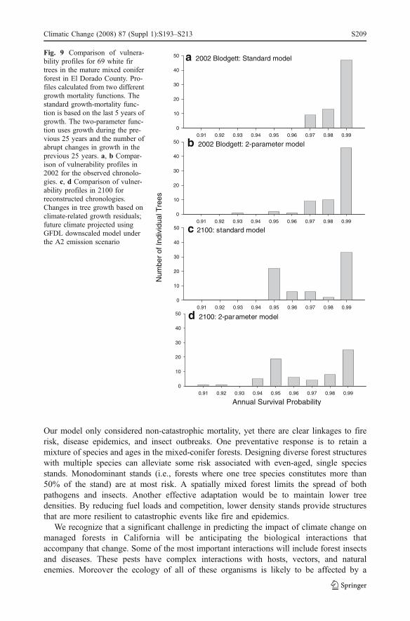
The predicted reductions in survival probability under future climates were slightly moresevere when survival was modeled using the two-parameter growth mortality function(Fig. 9). As noted above, growth reductions worsened with time. The two-parameter modelconsiders more of the growth record (25 years as opposed to 5) as well as any sharp annualdecreases that might occur in that period.

4 Discussion

4.1 Tree Growth

The four climate scenarios examined showed a distinct link between increasing summertemperatures and stem volume growth declines. Given the lack of any trend in the winter

Table 3 Cactosclim stem volume growth projections for single-tree selection management in a mixed-coniferforest in El Dorado County

Time Period aGFDL PCM

A2 B1 A2 B1

1971–2000 17.08 (1.80) 17.07 (1.78) 17.01 (1.88) 16.98 (1.88)2001–2030 15.91 (2.22) 16.52 (1.75) 16.65 (1.84) 17.08 (1.83)2036–2065 15.49 (1.53) 15.69 (1.59) 16.25 (1.80) 16.49 (1.74)2071–2100 13.69 (1.30) 15.12 (1.72) 15.45 (1.56) 16.19 (1.94)

a Climate simulations are based on downscaled results from two global climate models (GFDL and PCM)under two emission scenarios: A2 (higher CO2 emissions) and B1 (more moderate emission increases).Management interventions, ingrowth and mortality are tied to empirical results. Means with standard errorsin parentheses are based on average growth in each 30-year climate projection for two compartments (i.e., n=2). Units: m3 ha−1 year−1 . Mean volume growth is reported (m3 ha−1 year−1 ) followed by the standarderror in parentheses.

Table 4 Cactosclim stem volume growth projections for pine planation simulations (initial conditions=20 yr-old plantations) in El Dorado County

Time Period aGFDL PCM

A2 B1 A2 B1

1971–2000 11.95 (3.09) 11.95 (3.09) 11.84 (3.08) 11.82 (3.07)2001–2030 11.19 (2.97) 11.43 (3.01) 11.58 (3.03) 11.96 (3.09)2036–2065 10.54 (2.86) 10.69 (2.88) 11.20 (2.98) 11.48 (3.02)2071–2100 8.97 (2.60) 10.15 (2.80) 10.54 (2.86) 11.18 (2.97)

a Climate simulations are based on downscaled results from two global climate models (GFDL and PCM)under two emission scenarios: A2 (higher CO2 emissions) and B1 (more moderate emission increases).Means with standard errors in parentheses are based on average growth in each 30-year climate projection forsimulations with four different starting conditions (i.e., n=4). Units: m3 ha−1 year−1 . Mean volume growthis reported (m3 ha−1 year−1 ) followed by the standard error in parentheses.


precipitation patterns (Figs. 1 and 2), these summer temperatures were the drivers of change inthe CACTOSclim models. Summer drought is a typical aspect of the Mediterranean climateexperienced by the Sierran mixed-conifer forest. The intensity and extent of the moisturedeficit that develops during the summer are considered to be limiting factors in the growthand viability of Sierran conifers (Royce and Barbour 2001a). Higher summer temperatures ina Mediterranean climate (absent any changes in precipitation) could induce greater tree waterstress through higher evapotranspiration rates and/or faster depletion of moisture in the soilprofile. These changes would hasten the onset of drought stress that occurs in the late summerand early fall before the winter rains return. The result would be a shorter growing season dueto lack of moisture, which is already recognized as a primary growth constraint on mostcommercial timber sites in Sierran forests (Royce and Barbour 2001b).

30-yr Climate Predictions

Ste

m V

olum

e In

crem

ent (

m3 ha

-1yr

-1)

10

12

14

16

18

20

22

24

1970

1980

1990

20002000

2010

2020

2030

2035

2045

2055

2065

2070

2080

2090

2100

Fig. 6 Cactosclim growth projections for single-tree selection management in mixed conifer stands in El Doradocounty. Climate simulations based on the downscaled GFDL model under the A2 emission scenario. Means andstandard errors based on annual growth projection for the two single-tree compartments (i.e., n=2)


1970

1980

1990

2000

Ste

m V

olum

e In

crem

ent (

m3 ha

-1yr

-1)

13

15

17

19

21

23

25

27

2000

2010

2020

2030

2035

2045

2055

2065

2070

2080

2090

2100

Fig. 5 Cactosclim growth projections for reserve mixed-conifer stands in El Dorado county. Climatesimulations based on the downscaled GFDL model under the A2 emission scenario. Ingrowth and mortalitytied to empirical results. Means and standard errors based on annual growth projection for the four reservestands (i.e., n=4)


Given the relationship between tree growth and summer temperature, it was notsurprising that the most severe effects of projected climate change coincided with the mostsevere increases in temperature. The accelerated increase in summer temperature projectedfor 2071–2100 under the GFDL A2 scenario (Fig. 1) resulted in the most severe projectedreductions in tree growth for all management regimes (Tables 2, 3, and 4). Howevermanagement decisions clearly had an impact on the magnitude of the change.

Despite cultivating a species that is most tolerant of summer temperature (ponderosapine, Figs. 2 and 4), plantations showed the biggest relative loss of stem volume incrementand a comparable absolute loss of timber production. Silvicultural practices at least partiallyexplain this result. In the Sierra Nevada, pine plantations are typically harvested on a 50-year rotation. At the start of our 30-year simulation, the trees in a 20-year pine plantationwere on average smaller and younger than the trees in the reserve and single tree selectionstands. The pine plantations started with a lower initial volume of wood, and the trees alsospent a greater proportion of their life in the changed climate. In other words, there was less‘biological inertia’ in the pine plantations and thus the effects of climate change wereobserved more keenly.

A wealth of studies have modeled the impact of climate change on forest growth. Theresults vary by forest region, climate scenario, and modeling approach (reviewed inBugmann et al. 2001). While a definitive review is beyond the scope of this paper, recentresearch suggests that there may be a latitudinal trend in the response of upland coniferforests. In temperate latitudes, the growth of conifer forests more often declines underprojected future climates while productivity of conifer forests in boreal latitudes more oftenincreases (Linder 2000; Bugmann et al. 2001; Lasch et al. 2002; Briceño-Elizondo et al.2006). Our results follow this trend. Growth declined in this temperate conifer forest underevery management regime. Too few papers have addressed the interacting effects ofmanagement and climate change to draw any general conclusions other than to note thatforest management does influence the response (Linder 2000).

The magnitude and persistence of any changes in forest productivity related to changesin CO2 concentrations are crucial to projections of tree growth and yield. Biogeochemistry-based simulation models (e.g., CENTURY) predict increases in plant productivity underincreasing atmospheric CO2 (transpiration decreases thus improving water use efficiency).


Ste

m V

olum

e In

crem

ent (

m3 ha

-1yr

-1)

6

9

12

15

18

1970

1980

1990

20002000

2010

2020

2030

2035

2045

2055

2065

2070

2080

2090

2100

Fig. 7 Cactosclim growth projections for simulated ponderosa pine plantations typical of plantations in ElDorado county. Climate simulations based on the downscaled GFDL model under the A2 emission scenario.Means and standard errors based on annual growth projection for the four simulations (i.e., n=4)


Lenihan et al. (2003, 2006) include this CO2 fertilization-effect in their state-wide analysisof climate change effects on California vegetation. However growth chamber studies ofplant physiological response to increased CO2 routinely report photosynthetic acclimationimplying that any increases in productivity will be short-lived (Long et al. 2004). Resultsfrom the free air CO2 enrichment (FACE) experiments parallel some of the findings fromenclosure studies (Long et al. 2004) but a recent meta-analysis of FACE experimentssupport the contention that tree productivity does respond to CO2 enrichment (Ainsworthand Long 2005). For example in one of the longest FACE experiments with trees, Wittig etal. (2005) found significant increases in gross primary productivity for poplar coppiceplantations grown for three years in CO2 enriched environment. However, the increasedproductivity declined exponentially with time. By year three, gross productivity gainsranged from 5 to 19% (species-dependent) of the control. Interestingly Wittig et al. (2005)attributed the declines in productivity to light limitation (i.e., canopy closure) and notdown-regulation of photosynthesis. In contrast to the FACE meta-analysis, results from aweb-FACE study in a mature natural forest, where pure CO2 is released via a fine web oftubes woven into the tree canopies, showed no persistent stimulation in tree stem growth

Table 5 Annual survival probabilities for 69 Abies concolor trees sampled from the reserve stands atBlodgett Forest

aProjection scenario Target year

2002 2030 2065 2100

GFDL A2Mode 0.999 (48%) 0.999 (45%) 0.999 (39%) 0.956 (29%)25th 0.989 0.983 0.971 0.95650th 0.998 0.997 0.993 0.98375th 1.000 1.000 1.000 0.999GFDL B1Mode 0.999 (48%) 0.999 (48%) 0.999 (39%) 0.999 (39%)25th 0.991 0.987 0.976 0.97350th 0.998 0.997 0.994 0.99475th 1.000 1.000 1.000 1.000BFRS (current)Mode 0.999 (48%) – – –25th 0.987 – – –50th 0.997 – – –75th 1.000 – – –PCM A2Mode 0.999 (48%) 0.999 (48%) 0.999 (46%) 0.999 (39%)25th 0.988 0.989 0.985 0.96750th 0.998 0.998 0.997 0.99275th 1.000 1.000 1.000 0.999PCM B1Mode 0.999 (48%) 0.999 (45%) 0.999 (46%) 0.999 (48%)25th 0.991 0.987 0.986 0.98850th 0.998 0.997 0.997 0.99875th 1.000 1.000 1.000 1.000

a Projections based on absolute growth during the five years preceding the target year. Dendrochronologieswere adjusted for each climate scenario using the growth residual equations from Yeh and Wensel (2000).Mortality models fit for Abies concolor from growth and demography data from Sequoia Kings CanyonNational Park. Vulnerability profiles summarized using modal values and quantile distributions.


(Korner et al. 2005). Thus it remains an unresolved question whether the observed increasesin tree production under enriched CO2 translates into sustained increases in stem growth(Norby et al. 2005). Given our focus on wood production (i.e., stem growth) and the 30-year time frame adopted for this study, we did not include any CO2 fertilization effect in ourmodels. Clearly a better understanding of the long-term effects of climate change andatmospheric CO2 concentrations on tree water relations, forest productivity, and carbonallocation is crucial to improving projections of future forest conditions.

4.2 Tree mortality and forest health

No combination of climate scenarios and mortality models produced dramatic increases inwhite fir mortality (Table 5, Figs. 8 and 9). However the projected changes in climate couldexacerbate ongoing forest health concerns. The predicted reductions in growth increased thenumber of susceptible trees in the forest. Weak trees are less able to resist pathogeninfections and insect attacks, regardless of whether the pests are native or recently arrived.

Annual Survival Probability0.95 0.96 0.97 0.98 0.99

05

10152025303540455055

0.95 0.96 0.97 0.98 0.99

Num

ber

of In

divi

dual

Tre

es

05

10152025303540455055 0.95 0.96 0.97 0.98 0.99

05

10152025303540455055

0.95 0.96 0.97 0.98 0.9905

10152025303540455055 a 2002

b 2030

c 2065

d 2100

Fig. 8 a–d Shifts in annual sur-vival probability for 69 white firtrees in the mature mixed coniferforest in El Dorado county. Sur-vival probabilities based on pa-rameterized mortality functionusing the last five years of growth(i.e., standard model, see text).Changes in tree growth based onclimate-related growth residuals;projected climate using GFDLdownscaled predictions under A2emission scenario


Our model only considered non-catastrophic mortality, yet there are clear linkages to firerisk, disease epidemics, and insect outbreaks. One preventative response is to retain amixture of species and ages in the mixed-conifer forests. Designing diverse forest structureswith multiple species can alleviate some risk associated with even-aged, single speciesstands. Monodominant stands (i.e., forests where one tree species constitutes more than50% of the stand) are at most risk. A spatially mixed forest limits the spread of bothpathogens and insects. Another effective adaptation would be to maintain lower treedensities. By reducing fuel loads and competition, lower density stands provide structuresthat are more resilient to catastrophic events like fire and epidemics.

We recognize that a significant challenge in predicting the impact of climate change onmanaged forests in California will be anticipating the biological interactions thataccompany that change. Some of the most important interactions will include forest insectsand diseases. These pests have complex interactions with hosts, vectors, and naturalenemies. Moreover the ecology of all of these organisms is likely to be affected by a

0.91 0.92 0.93 0.94 0.95 0.96 0.97 0.98 0.99

Num

ber

of In

divi

dual

Tre

es

0

10

20

30

40

50

0.91 0.92 0.93 0.94 0.95 0.96 0.97 0.98 0.990

10

20

30

40

500.91 0.92 0.93 0.94 0.95 0.96 0.97 0.98 0.99

0

10

20

30

40

50 a 2002 Blodgett: Standard model

b 2002 Blodgett: 2-parameter model

d 2100: 2-parameter model

Annual Survival Probability

0.91 0.92 0.93 0.94 0.95 0.96 0.97 0.98 0.990

10

20

30

40

50 c 2100: standard model

Fig. 9 Comparison of vulnera-bility profiles for 69 white firtrees in the mature mixed coniferforest in El Dorado County. Pro-files calculated from two differentgrowth mortality functions. Thestandard growth-mortality func-tion is based on the last 5 years ofgrowth. The two-parameter func-tion uses growth during the pre-vious 25 years and the number ofabrupt changes in growth in theprevious 25 years. a, b Compar-ison of vulnerability profiles in2002 for the observed chronolo-gies. c, d Comparison of vulner-ability profiles in 2100 forreconstructed chronologies.Changes in tree growth based onclimate-related growth residuals;future climate projected usingGFDL downscaled model underthe A2 emission scenario


changing climate. Currently we are not capable of quantifying these crucial interactions.However we can discuss the most relevant issues for California’s forests.

Pest organisms have the ability to adapt much faster than their host trees, therebyincreasingly the likelihood of severe pest impact. Problems encountered with pestintroductions via global trade provide a cautionary example. As organisms move intonew but favorable habitats, potential for widespread damage is high because trees do notadapt quickly. Thus if a changing climate enables a pest to expand its range, the impactcould be similar to the introduction of an exotic pest. For example, pine pitch canker (anintroduced pathogen caused by Fusarium circinatum), once limited to coastal areas ofCalifornia, has expanded to the El Dorado National Forest in the Sierra Nevada (Vogler etal. 2004; Gordon 2005). If climate change results in more favorable environmentalconditions in the Sierra Nevada Mountains for pitch canker (e.g., milder winter minimumtemperatures), it could result in increased disease severity (all of the pine species in themixed-conifer forest are susceptible) and economic loss. In addition to the arrival of newpests, extant native organisms that rely on host stress may become more prevalent due tothe greater proportion of stressed trees (e.g., Fig. 8) in the population (Lonsdale and Gibbs1996). Specific examples relevant to California’s conifer forests include root diseasescaused by Armillaria spp. and certain wood or twig boring insects (Ips spp.).

4.3 Implications for timber management

All climate scenarios considered here were associated with decreasing volume growth andtimber yield. The responses available to offset declining yields in any specific region fallinto three categories. The most obvious is cutting more acreage to maintain constant totalyields. However, there are California regulatory restrictions on state and private lands thatpropose to cut more timber than can be replaced by growth. Any long term increases inharvest volume would need to come from federal lands which have been largely removedfrom the commercial timber base over the past decade or from other lands that have nottraditionally yielded timber products. Another response is to reduce investment in timbermanagement in order to increase net financial return. This strategy results in less intensiveforest management (e.g., reductions in shrub control, longer intervals between non-commercial thinning) that has implications for both forest health and fire risk. Alternatively,silvicultural treatments could be designed to compensate growth losses from climate changewith improvements in stand conditions. Planting mixtures of species, maintaining severalage classes, reducing tree density, and pruning trees at strategic intervals are examples ofcultural practices that could improve timber values but not necessarily timber yields.

4.4 Study limitations

All case studies are limited by the specificity of the particular case. In return, more detailed,and perhaps more reliable, information is obtained. However even for this site in El DoradoCounty where we had proven models and extensive data, we could only evaluate climatechange impacts on key forest parameters in isolation. But the processes of growth andmortality are fundamentally linked and the interaction will have direct effects on the forest’ssusceptibility to disease and insect attacks. Thus these processes must be studied in concertin order to properly forecast their role under a changed climate. Even within the modelingframework we defined, there are uncertainties in our projections. All results are limited bythe applicability of the CACTOS growth and yield model and the efficacy of thestatistically-fitted climate-growth residuals (Wensel et al. 1986, Yeh and Wensel 2000).


In addition, our implementation strategy had direct effects on our findings. On the onehand, we did not propagate through time the CACTOSclim results for the reserve stand. Byconstraining forest composition and structure, we potentially underestimated the con-sequences of climate change. On the other hand, we explicitly excluded CO2 fertilizationeffects – a decision that potentially leads to overestimates of productivity declines. We alsoused simulated stands to evaluate growth in pine plantations. At better alternative would beto ground the climate growth projections for pine plantations in inventory data as we did forthe reserve and single-tree analyses.

Modeling specific impacts of future climate on California’s forests is a precariousundertaking. In particular, we are concerned about the consequences of unanticipatedevents. We have only modeled the direct effects of climate change and not consideredpotential indirect effects on the disturbance regime (sensu Aber et al. 2001). Fire is anobvious concern. Insect outbreaks or pathogen irruptions also have the potential to entirelyswamp climate-related growth effects on forest yield and tree mortality. The nature,magnitude, and timing of these transforming events are difficult to predict. Unfortunatelywe will likely gain experience with these climate-driven transformations, and these eventswill provide crucial learning opportunities if we have built the informational andcomputational infrastructure needed to study them.

Acknowledgements We appreciate the critical reviews of earlier drafts of this work from Klaus Barber,Helge Eng, Guido Franco, Robert Heald, Gary Nakamura, Roger Sedjo, Lee Wensel, and two anonymousreviewers. Financial support for this project was provided by California Environmental Protection Agency,the USDA CREES Exotic/Invasive Pests and Disease Research Program, and the California AgriculturalExperiment Station.

References

Aber J, Neilson RP, McNulty S, Lenihan JM, Bachlet D, Drapek RJ (2001) Forest process and globalenvironmental change: predicting the effects of individual and multiple stressors. Bioscience 51:735–751

Ainsworth EA, Long SP (2005) What have we learned from 15 years of free-air CO2 enrichment (FACE)? Ameta-analytic review of the responses of photosynthesis, canopy properties and plant production to risingCO2. New Phytol 165:351–371

Anderson JL, Balaji V, Broccoli AJ, Cooke WF, Delworth TL, Dixon KW, Donner LJ, Dunne KA,Freidenreich SM, Garner ST, Gudgel RG, Gordon CT, Held IM, Hemler RS, Horowitz LW, Klein SA,Knutson TR, Kushner PJ, Langenhost AR, Lau NC, Liang Z, Malyshev SL, Milly PCD, Nath MJ,Ploshay JJ, Ramaswamy V, Schwarzkopf MD, Shevliakova E, Sirutis JJ, Soden BJ, Stern WF,Thompson LA, Wilson RJ, Wittenberg AT, Wyman BL (2004) The new GFDL global atmosphere andland model AM2-LM2: Evaluation with prescribed SST simulations. J Climate 17:4641–4673

Biging GS, Meerschaert W, Robards TA, Turnblom EC (1991) The Forest Stand Generator (STAG) User’sGuide Version 4.0. Research Note No. 34. http://www.cnr.berkeley.edu/~wensel/cactos/stag/stag.htm.Cited 16 May 2006

Bigler C, Bugmann H (2004) Predicting the time of tree death using dendrochronological data. Ecol Appl14:902–914

Briceño-Elizondo E, Garcia-Gonzalo J, Peltola H, Matala J, Kellomäki (2006) Sensitivity of growth of Scotspine, Norway spruce, and silver birch to climate change and forest management in boreal conditions. ForEcol Manag 232:152–167

Bugmann HKM, Wullschleger SD, Price DT, Ogle K, Clark DF, Solomon AM (2001) Comparing theperformance of forest gap models in North America. Clim Change 51:349–388

Cayan D, Maurer E, Dettinger M, Tyree M, Hayhoe K, Bonfils C, Duffy P, Santer B (2006) Climatescenarios for California. Public Interest Energy Research, California Energy Commission. CEC-500-2005-203-SF


http://www.cnr.berkeley.edu/~wensel/cactos/stag/stag.htm

Cherubini P, Fontana G, Rigling D, Dobbertin M, Brang P, Innes JL (2002) Tree-life history prior to death:two fungal root pathogens affect tree-ring growth differently. J Ecol 90:839–885

Das A, Battles JJ, Stephenson NL, van Mantgem PJ (2007) The relationship between tree growth patternsand likelihood of mortality: a study of two tree species in the Sierra Nevada. Can J For Res 37:580–597

Franklin JF, Fites-Kaufman JA (1996) Analysis of late successional forests. In: Sierra Nevada EcosystemProject: Final report to Congress, vol. II, chap. 21. Davis: University of California, Centers for Water andWildland Resources

FRAP (Fire and Resource Assessment Program) (2003) The Changing California: Forest and RangeAssessment 2003. Online technical report of the California Fire and Resource Assessment Program.http://frap.cdf.ca.gov/assessment2003/. Cited 10 October 2005

Gordon T (2005) The establishment of pitch canker in the Sierra Nevada. Poster at the UC Exotic/InvasivePest and Disease Research Program Workshop. University of California, Davis, 12 October 2005

Hayhoe K, Cayan D, Field CB, Frumhoff PC, Maurer EP, Miller NL, Moser SC, Schneider SH, Cahill KN,Cleland EE, Dale L, Drapek R, Hanemann RM, Kalkstein LS, Lenihan J, Lunch CK, Neilson RP,Sheridan SC, Verville JH (2004) Emissions pathways, climate change, and impacts on California. ProcNatl Acad Sci U S A 101:12422–12427

Johnsen K, Samuelson L, Teskey R, McNulty S, Fox T (2001) Process models as tools in forestry researchand management. For Sci 47:2–8

Kobe RK, Pacala SW, Silander JA, Canham CD (1995) Juvenile tree survivorship as a component of shadetolerance. Ecol Appl 5:517–532

Korner C, Asshoff R, Bignucolo O, Hattenschwiler S, Keel SG, Pelaez-Riedl S, Pepin S, Siegwolf RTW,Zotz G (2005) Carbon flux and growth in mature deciduous forest trees exposed to elevated CO2.Science 309:1360–1362

Lasch P, Linder M, Erhard M, Suckow F, Wenzel A (2002) Regional impact assessment on forest structureand functions under climate change – the Brandenburg case study. For Ecol Manag 162:73–86

Lenihan JM, Drapek R, Bachelet D, Neilson RP (2003) Climate change effects on vegetation distribution,carbon, and fire in California. Ecol Appl 13:1667–1681

Lenihan JM, Bachelet D, Drapek R, Neilson RP (2006) The response of vegetation distribution, ecosystemproductivity, and fire in California to future climate scenarios simulated by the MC1 DynamicVegetation Model. Public Interest Energy Research, California Energy Commission. CEC-500-2005-191-SF

Linder M (2000) Developing adaptive forest management strategies to cope with climate change. TreePhysiol 20:299–307

Long SP, Ainsworth EA, Rogers A, Ort DR (2004) Rising atmospheric carbon dioxide: Plants face the future.Annual Review Plant Biology 55:591–628

Lonsdale D, Gibbs JN (1996) Effects of climate change on fungal diseases of trees. In: Frankland JC, MaganM, Gadd GM (eds) Fungi and environmental change: symposium of the British Mycological Society,March 1994, Cranfield, England, UK. Cambridge University Press, Cambridge, UK

Meehl GA, Washington WM, Arblaster JM, Hu AX (2004) Factors affecting climate sensitivity in globalcoupled models. J Climate 17:1584–1596

Norby RJ, DeLucia EH, Gielen B, Calfapietra C, Giardina CP, King JS, Ledford J, McCarthy HR, MooreDJP, Ceulemans R, De Angelis P, Finzi AC, Karnosky DF, Kubiske ME, Lukac M, Pregitzer KS,Scarascia-Mugnozza GE, Schlesinger WH, Oren R (2005) Forest response to elevated CO2 is conservedacross a broad range of productivity. Proc Natl Acad Sci U S A 102:18052–18056

Olson CM, Helms JA (1996) Forest growth and stand structure at Blodgett Forest Research Station: 1933–95. In: Sierra Nevada Ecosystem Project: Final report to Congress, vol. III, chap. 16. Davis: Universityof California, Centers for Water and Wildland Resources

Pacala SW, Canham CD, Saponara J, Silander JA, Kobe RK, Ribbens E (1996) Forest models defined byfield measurements: Estimation, error analysis and dynamics. Ecol Monogr 66:1–43

Pedersen BS (1998) The role of stress in the mortality of midwestern oaks as indicated by growth prior todeath. Ecology 79:79–93

Royce EB, Barbour MG (2001a) Mediterranean climate effects. I. Conifer water use across a Sierra Nevadaecotone. Am J Bot 88:911–918

Royce EB, Barbour MG (2001b) Mediterranean climate effects. II. Conifer growth phenology across a SierraNevada ecotone. Am J Bot 88:919–932

Spelter H (2002) Conversion of board foot scaled logs to cubic meters in Washington State, 1970–1998.General Technical Report FPL-GTR-131. United States Department of Agriculture Forest Service, ForestProducts Laboratory, Madison, WI


http://frap.cdf.ca.gov/assessment2003/

Standiford R (2003) UCB Center for Forestry White Paper: The Forestry Program within the University ofCalifornia Division of Agriculture and Natural Resources. http://nature.berkeley.edu/forestry/. Cited 10October 2005

Suarez ML, Ghermandi L, Kitzberger T (2004) Factors predisposing episodic drought-induced tree mortalityin Nothofagus-site, climatic sensitivity and growth trends. J Ecol 92:954–966

Vogler DR, Gordon TR, Aegerter BJ, Kirkpatrick SC, Lunak GA, Stover P, Violett P (2004) First report ofthe pitch canker fungus (Fusarium circinatum) in the Sierra Nevada of California. Plant Dis 88(7):772

Wensel LC, Turnblom EC (1998) Adjustment of estimated tree growth rates in northern California conifersfor changes in precipitation levels. Can J For Res 28:1241–1248

Wensel LC, Daugherty PJ, Meerschaer WJ (1986) CACTOS User’ Guide: the California conifer timberoutput simulator. Bulletin 1920. Division of Agricultural Sciences University of California, Berkeley

Wittig VE, Bernacchi CJ, Zhu XG, Calfapietra C, Ceulemans R, Deangelis P, Gielen B, Miglietta F, MorganPB, Long SP (2005) Gross primary production is stimulated for three Populus species grown under free-air CO2 enrichment from planting through canopy closure. Glob Chang Biol 11:644–656

Wyckoff PH, Clark JS (2000) Predicting tree mortality from diameter growth: A comparison of maximumlikelihood and Bayesian approaches. Can J For Res 30:156–167

Yeh H-Y (1997) The relationship between tree diameter growth and climate for coniferous species innorthern California. Ph.D. dissertation, University of California, Berkeley

Yeh H-Y, Wensel LC (2000) The relationship between tree diameter growth and climate for coniferousspecies in northern California. Can J For Res 30:1463–1471

Yeh H-Y, Wensel LC, Turnblom EC (2000) An objective approach for classifying precipitation patterns tostudy climatic effects on tree growth. For Ecol Manag 139:41–50


http://nature.berkeley.edu/forestry/

climate change impacts on forest growth and tree mortality...

Documents