climate adaptation flagship working paper #13f

CLIMATE ADAPTATION FLAGSHIP

Generation of spatially downscaled climate change predictions for Australia Climate Adaptation Flagship Working Paper #13F

Tom Harwood, Kristen J Williams, Simon Ferrier

September 2012

National Library of Australia Cataloguing-in-Publication entry Title: Generation of spatially downscaled climate change predictions

for Australia / Tom Harwood

ISBN: 978-1-4863-0218-5 (pdf)

Series: CSIRO Climate Adaptation Flagship working paper series; 13F.

Other Authors/Contributors:

Climate Adaptation Flagship, Kristen J Williams, Simon Ferrier

Enquiries Enquiries regarding this document should be addressed to:

Tom Harwood

CSIRO Ecosystem Sciences

Black Mountain Laboratories, Clunies Ross Street

Black Mountain ACT 2601

[email protected]

Enquiries about the Climate Adaptation Flagship or the Working Paper series should be addressed to: Working Paper Coordinator

CSIRO Climate Adaptation Flagship

[email protected]

Citation Harwood T, Williams KJ and Ferrier S (2012) Generation of spatially downscaled climate change predictions for Australia. CSIRO Climate Adaptation Flagship Working Paper No. 13F. www.csiro.au/resources/CAF-working-papers

Copyright and disclaimer © 2012 CSIRO To the extent permitted by law, all rights are reserved and no part of this publication covered by copyright may be reproduced or copied in any form or by any means except with the written permission of CSIRO.

Important disclaimer CSIRO advises that the information contained in this publication comprises general statements based on scientific research. The reader is advised and needs to be aware that such information may be incomplete or unable to be used in any specific situation. No reliance or actions must therefore be made on that information without seeking prior expert professional, scientific and technical advice. To the extent permitted by law, CSIRO (including its employees and consultants) excludes all liability to any person for any consequences, including but not limited to all losses, damages, costs, expenses and any other compensation, arising directly or indirectly from using this publication (in part or in whole) and any information or material contained in it.

mailto:[email protected]

http://www.csiro.au/resources/CAF-working-papers


The Climate Adaptation Flagship Working Paper series The CSIRO Climate Adaptation National Research Flagship has been created to address the urgent national challenge of enabling Australia to adapt more effectively to the impacts of climate change and variability.

This working paper series aims to:

• provide a quick and simple avenue to disseminate high-quality original research, based on work in progress

• generate discussion by distributing work for comment prior to formal publication.

The series is open to researchers working with the Climate Adaptation Flagship on any topic relevant to the Flagship’s goals and scope.

Copies of Climate Adaptation Flagship Working Papers can be downloaded at:

www.csiro.au/resources/CAF-working-papers

CSIRO initiated the National Research Flagships to provide science-based solutions in response to Australia’s major research challenges and opportunities. Flagships form multidisciplinary teams with industry and the research community to deliver impact and benefits for Australia.


CSIRO Climate Adaptation Flagship Working Paper 13F • September 2012 | i

Contents

Acknowledgments ............................................................................................................................................. iii

Executive summary............................................................................................................................................ iv

1 Introduction .......................................................................................................................................... 1 1.1 Summary of approach ................................................................................................................. 1

2 ‘Present’ climate and base climates ...................................................................................................... 3

3 Future climate surfaces ......................................................................................................................... 4 3.1 Role in ANCULIM 6.0 development cycle ................................................................................... 5 3.2 Generation of Change Grids for input to ANUCLIM 6.0 .............................................................. 5 3.3 CSIRO OzConverter ..................................................................................................................... 7 3.4 Downscaled outputs from ANUCLIM 6 ....................................................................................... 7 3.5 Assessment of BIOCLIM surfaces for use in climate change studies .......................................... 8

Conclusion ........................................................................................................................................................ 11

References ........................................................................................................................................................ 12

ii | CSIRO Climate Adaptation Flagship Working Paper 13F • September 2012

Figures Figure 1 Spatial downscaling of future climate scenarios using ANUCLIM 6.0 .................................................. 4

Figure 2 Typical overlay of 0.25° OzClim files over the 0.01° DEM on wgs84, Darwin region, showing the incomplete edge coverage of the raw OzClim files. Black = no data, yellow= DEM, blues= OzClim ................. 5

Figure 3 Extension (red) of OzClim files (blue) required to cover the whole country ........................................ 6

Figure 4 Converting OzClim Evapotranspiration file for input to ANUCLIM 6 .................................................... 7

Figure 5 Examples of spatial anomalies generated in ANUCLIM 6 as seen in the variables listed in Table 3, shown for a) Bio9 2070H, multiple anomalies; and b) Bio21 2070H, XY starring under climate change caused by OzClim downscaling ......................................................................................................................... 10

Tables Table 1 Collection period and effective base dates for the climate surfaces with ANUCLIM v5.1 cf. v6 .......... 3

Table 2 BIOCLIM parameters likely to be robust for use in climate change studies .......................................... 8

Table 3 BIOCLIM parameters unsuitable for use in climate change studies. Parameters are ranked: x = meaningful patterns, but likely to cause problems under climate change; xx = spatially unlikely patterns, where the wettest quarter shifts dramatically between adjacent cells; xxx = complex effects which may be due to problems in the basic definition or application of the parameters. Short descriptions are given .... 9

CSIRO Climate Adaptation Flagship Working Paper 13F • September 2012 | iii

Acknowledgements

We are grateful to Mike Hutchinson and Tingbao Xu at the ANU Fenner School of Environment and Society for their advice on the approaches used, and for the use and modification of the beta version of ANUCLIM 6.

The project was supported by all Australian governments through the Climate Change in Agriculture and NRM (CLAN) Working Group of the Natural Resource Management Ministerial Council, the Australian Government Department of Sustainability, Environment, Water, Population and Communities (DSEWPaC), and the Department of Climate Change and Energy Efficiency (DCCEE). The project was co-funded by CSIRO Climate Adaptation Flagship.

We thank Ruth Davies of centrEditing for editing this report.

iv | CSIRO Climate Adaptation Flagship Working Paper 13F • September 2012

Executive summary

This working paper documents a straightforward approach for the spatial downscaling of coarse resolution Global Circulation Model outputs to finer scales (in this case approximately 1 km2), which is suitable for Australia. The work here contributed directly to an analysis of the future of the National Reserve System but is broadly applicable and has been subsequently applied at different spatial scales.

Global Circulation Models produce projections of climate change at fairly coarse grid scales which are inadequate for the representation of many biological processes. The OzClim portal allows the user to download climate projections which have been rigorously downscaled to a 0.25° (25 km) resolution. Here we describe the use of these data as inputs to ANUCLIM software to further statistically downscale the projections based on current climate surfaces and height above sea level. Issues relating to the successful integration of these two data sources are critically assessed and solutions described in detail where appropriate. The approach is transparent, theoretically sound and produces coherent results.

CSIRO Climate Adaptation Flagship Working Paper 13F • September 2012 | 1

1 Introduction

This report describes work contributing to the CSIRO analysis of the effects of climate change on Australian biodiversity and the implications of this for the National Reserve System (NRS) (Dunlop et al. 2012; Ferrier et al. 2012). Prerequisites for this study were suites of environmental surfaces for both the present climate and future climate scenarios on which to base the modelling. This report describes the generation of future climate surfaces conducted for this purpose. These surfaces were collated for mainland Australia and nearby offshore islands within a bounding box -43.8°N to -9.0°N, 111.875°E to 154.5°E, at a resolution of 0.01° (approx 1 km2). The choice of surfaces was based upon those used in Williams et al. (2010) in the Caring for our Country project, which in turn were based on the review of national environmental datasets by Stein (2008). The Caring for our Country project informed the choice of scale, since the GDM models used in the current study were developed in Williams et al. 2010 at a 0.01° resolution (approx. 1 km2). It should be noted that the climatic variables form a subset of the total environmental surfaces used in the GDM modelling approach. The ANN modelling studies required the generation of climate surfaces at 0.02°resolution.

Extensive downscaling from the raw output of a Global Circulation Model (GCM) was required to derive 0.01° grids that reflect the potential impacts of future climate which are essential to the assessment of the future of the NRS. There is a high degree of uncertainty both in the underlying climate surfaces for Australia and in the outputs of GCMs. As such there will be inherent uncertainties in any downscaling approach. However, in the context of this study it was considered appropriate to attempt to capture both the broad properties of the changing climate, and the finer-scale modifications of this by topography. The approach we decided upon was one devised at ANU, taking the 0.25° outputs of the CSIRO OzClim website in terms of change relative to the base climate surfaces, and overlaying these on current climate surfaces interpolated from weather station records using a combination of splined interpolation and lapse rate correction based on a supplied Digital Elevation Model (Hutchinson et al. 2008). We used the beta version 6 of ANUCLIM (Houlder et al. 2000). This represents a straightforward and relatively transparent approach to spatial downscaling, which may be criticised on the uncertainties in the inputs, but is directly compatible with the datasets of Stein (2008).

Two scenarios were considered, both using outputs from the CSIRO Mk3.5 GCM from OzClim (CSIRO 2012). The CSIRO GCM is ranked in the top 15 GCMs for Australia in Suppiah et al. (2007) and provides the required outputs (Minimum and Maximum Temperature, Rainfall and Areal Potential Evaporation). These scenarios were couched in terms of their impact on the future NRS: a medium impact scenario, using the A1B emissions scenario; and a high impact scenario using the A1FI emissions scenario (IPCC 2000). The main future date considered was 2070, although an intermediate 2030 scenario was also developed.

1.1 Summary of approach

The first step was to download monthly climate change grids at 0.25° resolution for maximum temperature, minimum temperature, rainfall and evaporation, by specifying the above scenarios in OzClim. Spatial downscaling was carried out using the ANUCLIM software (Houlder et al. 2000), which incorporates three submodels: ESOCLIM, which outputs raw climate variable grids; BIOCLIM (Busby 1986), which outputs grids of bioclimatic parameters; and GROCLIM, which can output gridded indices from simple growth models. The beta release of ANUCLIM version 6.0 was used, which allows climate change grids to be applied over the historical 1990-centred climate surfaces. Software (Harwood and Williams 2009) was written to interpolate the raw 0.25° CSIRO grids to cover the whole Australian land mass and relate evaporation change to the date range used in ANUCLIM 6. Following this interpolation, monthly maximum temperature, minimum temperature, rainfall, and evaporation change grids were input into ANUCLIM 6 with a 0.01° digital elevation model. The result was a suite of monthly 0.01° (≈1 km2) resolution future climate surfaces

2 | CSIRO Climate Adaptation Flagship Working Paper 13F • September 2012

for maximum temperature, minimum temperature, rainfall, pan evaporation and radiation, with 35 BIOCLIM variables and four plant growth indices for each scenario. An analysis of the spatio-temporal performance of the BIOCLIM variables under climate change was conducted, and the list subsequently reduced to 23 BIOCLIM variables to avoid data anomalies. Further to this, additional climate descriptors were developed in accordance with the approaches used in Williams et al. 2010.


2 ‘Present’ climate and base climates

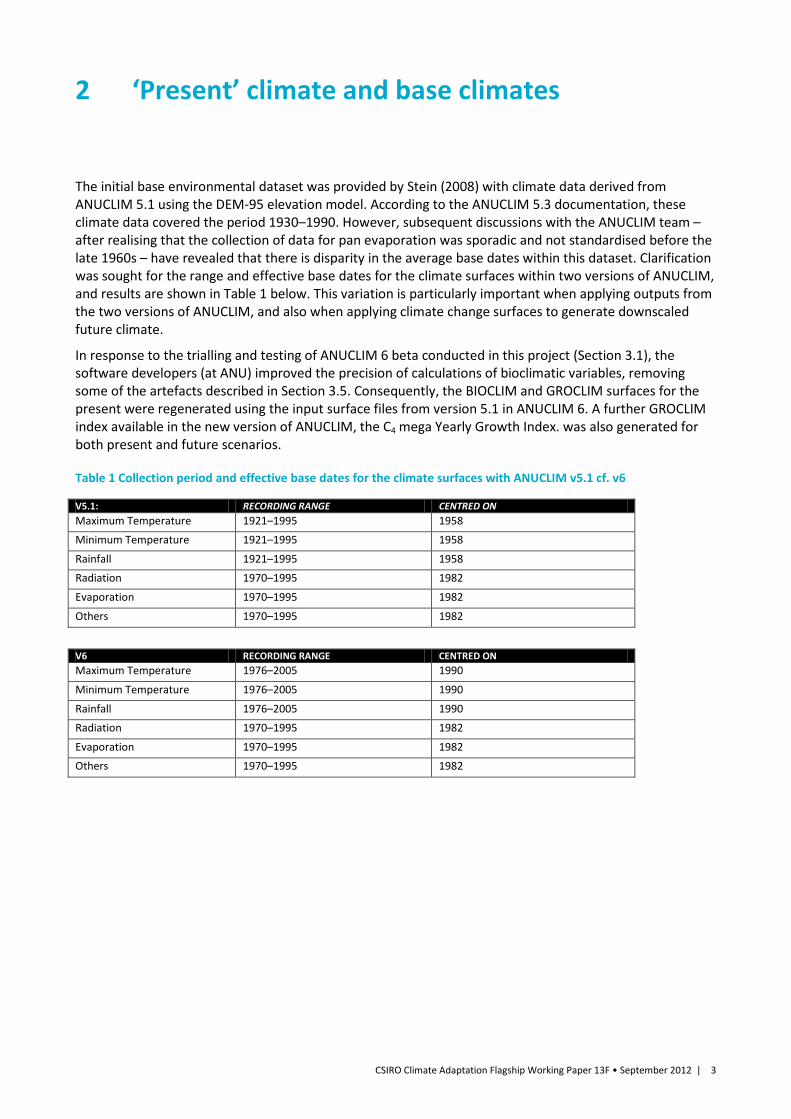
The initial base environmental dataset was provided by Stein (2008) with climate data derived from ANUCLIM 5.1 using the DEM-95 elevation model. According to the ANUCLIM 5.3 documentation, these climate data covered the period 1930–1990. However, subsequent discussions with the ANUCLIM team – after realising that the collection of data for pan evaporation was sporadic and not standardised before the late 1960s – have revealed that there is disparity in the average base dates within this dataset. Clarification was sought for the range and effective base dates for the climate surfaces within two versions of ANUCLIM, and results are shown in Table 1 below. This variation is particularly important when applying outputs from the two versions of ANUCLIM, and also when applying climate change surfaces to generate downscaled future climate.

In response to the trialling and testing of ANUCLIM 6 beta conducted in this project (Section 3.1), the software developers (at ANU) improved the precision of calculations of bioclimatic variables, removing some of the artefacts described in Section 3.5. Consequently, the BIOCLIM and GROCLIM surfaces for the present were regenerated using the input surface files from version 5.1 in ANUCLIM 6. A further GROCLIM index available in the new version of ANUCLIM, the C4 mega Yearly Growth Index. was also generated for both present and future scenarios.

Table 1 Collection period and effective base dates for the climate surfaces with ANUCLIM v5.1 cf. v6

V5.1: RECORDING RANGE CENTRED ON Maximum Temperature 1921–1995 1958

Minimum Temperature 1921–1995 1958

Rainfall 1921–1995 1958

Radiation 1970–1995 1982

Evaporation 1970–1995 1982

Others 1970–1995 1982

V6 RECORDING RANGE CENTRED ON Maximum Temperature 1976–2005 1990

Minimum Temperature 1976–2005 1990

Rainfall 1976–2005 1990

Radiation 1970–1995 1982

Evaporation 1970–1995 1982

Others 1970–1995 1982


3 Future climate surfaces

Future climate surfaces were generated at a 0.01° resolution for the whole country lying within a bounding box: -43.8°N to -9.0°N, 111.875°E to 154.5°E to ensure coverage of the mainland and coastal islands, including the Torres Strait Islands. Restrictions on other data grids subsequently reduced the areal coverage, but it was deemed appropriate to generate new data to maximise national coverage.

Figure 1 shows the spatial downscaling process as applied in ANUCLIM 6.0. After selecting a Digital Elevation model at the required output scale, the software is provided with gridded Change Grids for each month of the year.

Figure 1 Spatial downscaling of future climate scenarios using ANUCLIM 6.0

These layers are downscaled, using the historical climate surfaces within ANUCLIM 6.0 (with dates as shown Table 1). Change Grids can be provided for Maximum Temperature and Minimum Temperature in units +/- °C and for Rainfall and Evaporation in units +/- % change. Change is therefore measured relative to the appropriate base year as shown in Table 1.

Changes in monthly Radiation were generated by using the ‘Radiation with Rainfall’ option in ANUCLIM, rather than by supplying gridded Change Grids, as used for the other changing variables. This approach allows future rainfall and radiation to be better correlated and was recommended by the software developers at ANU.

0.01º DEM

Historical climate 0.25º change grid

0.01º Future climate

+


3.1 Role in ANCULIM 6.0 development cycle

ANUCLIM 6.0 was still in its pre-release beta version at the time of use, and has limited help files available. As such, the development of the approaches below required extensive product testing and debugging, and subsequent regeneration of input grids and results following discussion with the software developers. While most changes made to the software under development resulted in bug removal and the software functioning as it should, critical appraisal of the discontinuities in BIOCLIM has also led to improved precision.

3.2 Generation of Change Grids for input to ANUCLIM 6.0

Climate scenarios were downloaded from OzClim (CSIRO 2012), using the Advanced download page, which allows specification of the GCM, emissions scenario, and climate sensitivity. Two scenarios rated for their impact on the NRS were used, generated from the CSIRO Mk3.5 GCM:

• High Impact: A1FI emissions scenario, High climate sensitivity • Medium Impact: A1B emissions scenario, Medium climate sensitivity.

Monthly 0.25° grids were downloaded for two future dates, 2030 and 2070, as follows:

• Maximum Temperature: +/-°C change from 1990 base date • Minimum Temperature: +/-°C change from 1990 base date • Rainfall: +/-% change from 1990 base date • Evapotranspiration: Future climate.

While the first three variables are provided by OzClim as change from the same base date (1990) as that used in ANUCLIM 6, the Evapotranspiration variable requires explicit treatment in order to generate the appropriate change from a 1982-centred dataset (Table 1) prior to input to ANUCLIM.

The following steps were therefore taken in the development of the 0.25° Change Grids for input to ANUCLIM.

3.2.1 EXTENSION OF OZCLIM FILES TO COVER THE WHOLE COUNTRY

The 0.25° OzClim output files do not cover the whole of Australia. They leave gaps around the edges (Figure 2). They therefore required extension in order to provide a satisfactory input to ANUCLIM 6, which allows the generation of 0.01° resolution climate surfaces based on the OzClim future scenarios.

Figure 2 Typical overlay of 0.25° OzClim files over the 0.01° DEM mask, Darwin region, showing the incomplete edge coverage of the raw OzClim files. Black = no data, yellow= DEM, blues= OzClim


Approach

Step 1: A 0.25° Boolean mask file was created to cover the whole country. NO_DATA= Sea; 1= square occupied by some Australian land by overlaying 9 second DEM over a 0.25º grid with the same origin as the raw OzClim files. Using bespoke software Borland C++ Builder. Saved as ‘Australia25km.asc’.

Step 2: For each monthly file for each climate variable the raw OzClim file was interpolated to cover the whole Australia25km mask.

a) where covered in the raw OzClim file, data were copied straight across.

For all cells in Australia25km.asc which are not covered by the original OzClim file:

b) where there were one or more cells in the 8-cell Moore neighbourhood in the raw OzClim file, the value was taken as the mean of those cells.

c) where there were no local neighbours, a search was conducted outwards to find the nearest cell in the OzClim file. If more than one cell had the same distance, the mean of these nearest cells was used.

d) Output files were referenced to xllcenter /yllcenter, with carriage returns at the end of each line and, critically, at the end of the file for ANUCLIM compatibility.

Figure 3 Extension (red) of OzClim files (blue) required to cover the whole country

3.2.2 GENERATING EVAPORATION FILES

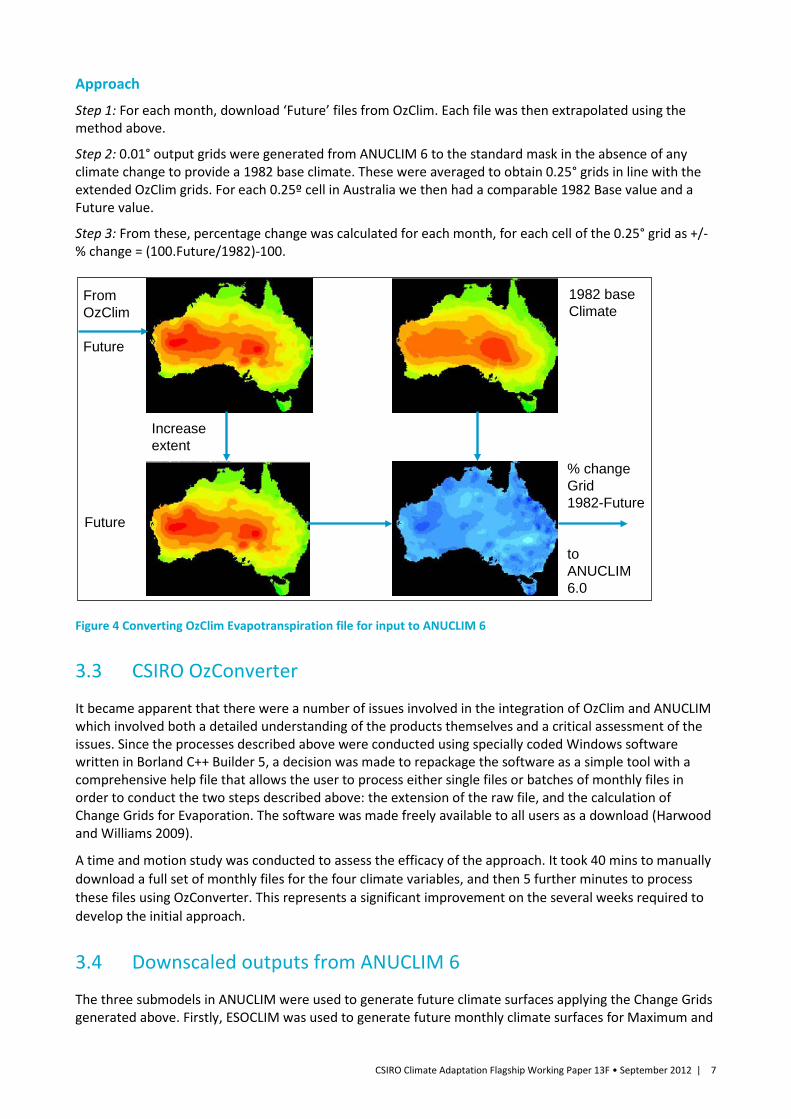
Special consideration had to be given to the treatment of evaporation surfaces, due to issues of incompatibility in the outputs from OzClim and the input requirements of ANUCLIM, which were not relevant for the other variables. The ANUCLIM 6 Pan Evaporation surface is centred on 1982, and requires inputs in units of % change from the base date. The required Change Grid is therefore +/- % change from 1982 to 2030/2070. OzClim only produces results for Areal Potential Evaporation in two formats: ‘Future’ and ‘Change from Base (1990)’, so we worked with the Future scenario and the 1982 ESOCLIM output surfaces from ANUCLIM 6 (Figure 4). It was assumed that change in Pan Evaporation was directly comparable with changes in Areal Potential Evaporation.


Approach Step 1: For each month, download ‘Future’ files from OzClim. Each file was then extrapolated using the method above.

Step 2: 0.01° output grids were generated from ANUCLIM 6 to the standard mask in the absence of any climate change to provide a 1982 base climate. These were averaged to obtain 0.25° grids in line with the extended OzClim grids. For each 0.25º cell in Australia we then had a comparable 1982 Base value and a Future value.

Step 3: From these, percentage change was calculated for each month, for each cell of the 0.25° grid as +/-% change = (100.Future/1982)-100.

Figure 4 Converting OzClim Evapotranspiration file for input to ANUCLIM 6

3.3 CSIRO OzConverter

It became apparent that there were a number of issues involved in the integration of OzClim and ANUCLIM which involved both a detailed understanding of the products themselves and a critical assessment of the issues. Since the processes described above were conducted using specially coded Windows software written in Borland C++ Builder 5, a decision was made to repackage the software as a simple tool with a comprehensive help file that allows the user to process either single files or batches of monthly files in order to conduct the two steps described above: the extension of the raw file, and the calculation of Change Grids for Evaporation. The software was made freely available to all users as a download (Harwood and Williams 2009).

A time and motion study was conducted to assess the efficacy of the approach. It took 40 mins to manually download a full set of monthly files for the four climate variables, and then 5 further minutes to process these files using OzConverter. This represents a significant improvement on the several weeks required to develop the initial approach.

3.4 Downscaled outputs from ANUCLIM 6

The three submodels in ANUCLIM were used to generate future climate surfaces applying the Change Grids generated above. Firstly, ESOCLIM was used to generate future monthly climate surfaces for Maximum and

FromOzClim

Future

Increase extent

1982 baseClimate

% changeGrid1982-Future

to ANUCLIM 6.0

Future


Minimum Temperature, Rainfall, Evaporation and Radiation (using Radiation with rainfall). BIOCLIM was used to generate the 35 standard bioclimatic variables, and GROCLIM to generate Yearly Growth Indices for C3 microtherms, mesotherms and megatherms (as in Williams et al. 2010), with the additional C4 megatherm output. Following the improvement of precision in the BIOCLIM calculations in response to our queries, the 1960 BIOCLIM variables were regenerated by loading the 1960-centred climate surfaces (ANUCLIM 5.1) into ANUCLIM 6. A 1960 base C4 megatherm surface was also generated.

3.5 Assessment of BIOCLIM surfaces for use in climate change studies

BIOCLIM’s bioclimatic variables attempt to summarise complex temporal effects of climatic conditions, distilling them to 35 parameters. These involve both the definition of extreme quarters, and the calculation of specific indices. When applied to a single point, these parameters have proved to be useful biological indicators. However, extending the application to large-scale spatial studies reveals spatial artefacts in the form of granularities and discontinuities in the outputs that are due to a number of factors, such as input and output data precision, the inherent nature of the variables (wettest and driest quarters do not change continuously across Australia), and potentially to the weekly units currently used in the definition of quarters. These may not be problematic in static studies, but when used for climate change studies, where the difference between output grids over space becomes important, any discrete patterning (such as contouring due to low data precision) is exacerbated. Critical assessment of the applicability of each parameter was carried out. ANUCLIM 6 beta (December 2009) with updated data precision was examined for discontinuities under both date bases and for several future climate scenarios (Table 2).

Table 2 BIOCLIM parameters likely to be robust for use in climate change studies

bio1 Annual Mean Temperature (°C) bio2 Mean Diurnal Range(Mean(period max-min)) (°C) bio3 Isothermality bio4 Temperature Seasonality (C of V) bio5 Max Temperature of Warmest Period (°C) bio6 Min Temperature of Coldest Period (°C) bio7 Temperature Annual Range (°C) bio10 Mean Temperature of Warmest Quarter (°C) bio11 Mean Temperature of Coldest Quarter (°C) bio12 Annual Precipitation (mm) bio13 Precipitation of Wettest Period (mm) bio14 Precipitation of Driest Period (mm) bio15 Precipitation Seasonality (C of V) bio16 Precipitation of Wettest Quarter (mm) bio20 Annual Mean Radiation (MJ.m-2day-1) bio21 Highest Period Radiation (MJ.m-2day-1) bio22 Lowest Period Radiation (MJ.m-2day-1) bio23 Radiation Seasonality (C of V) bio28 Annual Mean Moisture Index bio29 Highest Period Moisture Index bio30 The minimum moisture index value for all weeks bio31 Moisture Index Seasonality (C of V) bio32 Mean Moisture Index of Highest Quarter MI bio33 Mean Moisture Index of Lowest Quarter MI bio35 Mean Moisture Index of Coldest Quarter

Note that this is a beta version of the software and the full release may rectify some of the issues. Radiation was generated as ‘radiation from rainfall’ as recommended by the authors.


Both raw and transformed (Logarithmic, Linear stretch, Equalisation enhancement in OpenEV GIS) data were examined. The output grids which showed continuous distributions of parameters across the continent, and which are likely therefore to be useful for the examination of climate change, are listed in Table 2. It should be borne in mind that specific scenarios, uses or transformations may highlight problems with these parameters, although they are generally robust. In particular, where the differences between cells are at the limits of the precision of the data, some contouring may be generated.

The grids below (Table 3) may be considered unsuitable for climate change studies where detailed spatial analysis is required. Examples of spatial patterning under climate change are shown in Figure 5. This may be due to contouring problems due to low data precision relative to the output grids, spatial discontinuities (particularly with regards water, and consequently with regards radiation, since this is in this case derived from rainfall), and unexpected patterning, possibly due to limitations in the base algorithms.

Outputs for bio15 and bio21 are generally continuous and reasonable. However, at high rates of change (e.g. A1FI 2070) a subtle vertical and horizontal striping pattern emerges in some areas (Figure 5b). This change appears to derive from the initial downscaling in OzClim, and should not be attributed to the ANUCLIM downscaling process. We excluded these layers from our modelling analyses, but recommend them for use where the underlying data are reliable.

Table 3 BIOCLIM parameters unsuitable for use in climate change studies. Parameters are ranked: x = meaningful patterns, but likely to cause problems under climate change; xx = spatially unlikely patterns, where the wettest quarter shifts dramatically between adjacent cells; xxx = complex effects which may be due to problems in the basic definition or application of the parameters. Short descriptions are given

CODE DESCRIPTION RANK SPATIAL ARTEFACTS bio8 Mean Temperature of Wettest Quarter (°C) xx strong discontinuities bio9 Mean Temperature of Driest Quarter (°C) xxx multiple anomalies bio17 Precipitation of Driest Quarter (mm) x discontinuities when transformed bio18 Precipitation of Warmest Quarter (mm) x contouring bio19 Precipitation of Coldest Quarter (mm) x discontinuities when transformed bio24 Radiation of Wettest Quarter (MJ.m-2day-1) xx strong discontinuities bio25 Radiation of Driest Quarter (MJ.m-2day-1) xxx multiple anomalies bio26 Radiation of Warmest Quarter (MJ.m-2day-1) x contouring bio27 Radiation of Coldest Quarter (MJ.m-2day-1) x contouring bio34 Mean Moisture Index of Warmest Quarter x contouring


a)

b)

Figure 5 Examples of spatial anomalies generated in ANUCLIM 6 as seen in the variables listed in Table 3, shown for a) Bio9 2070H, multiple anomalies; and b) Bio21 2070H, XY starring under climate change present in OzClim downscaling


Conclusion

The approach described above is a repeatable transparent method, which is fit for purpose. Advances in both OzClim and ANUCLIM must be taken into account when applying this methodology in the future and care should always be taken regarding base climate dates as described here. The introduction of further terrain adjustment in terms of radiative balance and surface/groundwater flow is worthy of consideration as a next stage of downscaling, although all approaches need to be consistent with the assumptions and outputs of Global Circulation Models.


References

Busby JR (1986) Bioclimate Prediction System (BIOCLIM) User’s Manual. Version 2.0. Bureau of Flora and Fauna, Canberra.

CSIRO (2012) OzClim. Exploring climate change scenarios for Australia. http://www.csiro.au/ozclim.

Dunlop M, Hilbert DW, Ferrier S, House A, Liedloff A, Prober SM, Smyth A, Martin TG, Harwood T, Williams KJ, Fletcher C and Murphy H (2012) The Implications of Climate Change for Biodiversity Conservation and the National Reserve System: Final Synthesis. A report prepared for the Department of Sustainability, Environment, Water, Population and Communities, and the Department of Climate Change and Energy Efficiency. CSIRO Climate Adaptation Flagship, Canberra.

Ferrier S, Harwood T and Williams KJ (2012) Using Generalised Dissimilarity Modelling to assess potential impacts of climate change on biodiversity composition in Australia, and on the representativeness of the National Reserve System. CSIRO Climate Adaptation Flagship Working Paper No. 13E. http://www.csiro.au/en/Organisation-Structure/Flagships/Climate-Adaptation-Flagship/CAF-working-papers.aspx.

Harwood T and Williams KJ (2009) CSIRO OzConverter: Edit 0.25° OzClim *.asc output files. http://www.csiro.au/products/OzConverter-Software.html.

Houlder DJ, Hutchinson MF, Nix HA and McMahon JP (2000) ANUCLIM User Guide, Version 5.1. Centre for Resource and Environmental Studies, Australian National University, Canberra. http://www.fennerschool.anu.edu.au/publications/software/anuclim.php.

Hutchinson M, Stein J, Stein J, Anderson H and Tickle P (2008) GEODATA 9 Second DEM and D8 Digital Elevation Model Version 3 and Flow Direction Grid Gridded Elevation and Drainage Data Source Scale 1:250 000, User Guide. Fenner School of Environment and Society, ANU and Geoscience Australia, Canberra.

IPCC (2000) Emissions Scenarios. Special Report of the Intergovernmental Panel on Climate Change. Eds. Nakicenovic N and Swart R. Cambridge University Press. Cambridge. UK.

Stein J (2008) Metadata: Environmental attributes compiled for the continental GDM analysis. Fenner School of Environment and Society, Australian National University, Canberra.

Suppiah R, Hennessy KJ, Whetton PH, McInnes K, Macadam I, Bathols J, Ricketts J and Page CJ (2007) Australian Climate change projections derived from simulations performed for the IPCC 4th Assessment Report. Australian Meteorological Magazine 56(3), 131–152.

Williams KJ, Ferrier S, Rosauer D, Yeates D, Manion G, Harwood T, Stein J, Faith DP, Laity T and Whalen A (2010) Harnessing continent-wide biodiversity datasets for prioritising national conservation investment. A report to the Department of Environment, Water, Heritage and the Arts. CSIRO, Canberra.

http://www.csiro.au/ozclim

http://www.csiro.au/en/Organisation-Structure/Flagships/Climate-Adaptation-Flagship/CAF-working-papers.aspx

http://www.csiro.au/en/Organisation-Structure/Flagships/Climate-Adaptation-Flagship/CAF-working-papers.aspx

http://www.csiro.au/products/OzConverter-Software.html

http://www.fennerschool.anu.edu.au/publications/software/anuclim.php


CONTACT US t 1300 363 400 +61 3 9545 2176 e [email protected] w www.csiro.au

YOUR CSIRO Australia is founding its future on science and innovation. Its national science agency, CSIRO, is a powerhouse of ideas, technologies and skills for building prosperity, growth, health and sustainability. It serves governments, industries, business and communities across the nation.

FOR FURTHER INFORMATION Ecosystem Sciences Tom Harwood t +61 2 6246 4018 e [email protected] w www.csiro.au/people/Tom.Harwood

mailto:[email protected]

http://www.csiro.au/people/Tom.Harwood

climate adaptation flagship working paper #13f

Documents