click here to return to usgs publications · principle of superposition 19 metric conversion...

Click here to return to USGS publications

http://www.usgs.gov

../index.html

The Effects of Boundary Conditions onthe Steady-State Response of ThreeHypothetical Ground-Water Systems-Results and Implications of NumericalExperiments

By O . Lehn Franke and Thomas E . Reilly

U .S . GEOLOGICAL SURVEY WATER-SUPPLY PAPER 2315

DEPARTMENT OF THE INTERIOR

MANUEL LUJAN, Jr ., Secretary

U .S . GEOLOGICAL SURVEY

Dallas L . Peck, Director

Any use of trade, product, or firm names in this publication is for descriptive purposesonly and does not imply endorsement by the U.S . Government

First printing 1987Second printing 1990

UNITED STATES GOVERNMENT PRINTING OFFICE : 1987

For sale by theBooks and Open-File Reports SectionU.S . Geological SurveyFederal Center, Box 25425Denver, CO 80225

Library of Congress Cataloging in Publication Data

Franke, O . Lehn .The effects of boundary conditions on the steady-state response of threehypothetical ground-water systems-results and implications of numericalexperiments.(U .S . Geological Survey water-supply paper ; 2315)Bibliography ; p.Supt . of Docs . no . :

1 19 :13:23151 . Water, Underground-Mathematical models .

2. Water, Underground-Simulation methods.

3. Groundwater flow-Mathematical models .

4.Groundwater flow-Simulation methods .

1 . Reilly, Thomas E .

If . Title .111 . Series .

GB1001 .72.M35F73 1987 55379'0724 86-600382

CONTENTS

Metric conversion factors ivAbstract 1Introduction 1Description of three hypothetical ground-water systems

2Effects of boundary conditions on the steady-state response of the three hypo-

thetical ground-water systems 3Description of numerical experiments

3Results of numerical experiments

3Series A experiments

3Series B experiments 5Series C experiments 6

Implications of numerical experiments for simulation of ground-watersystems 8

Model calibration 8Solute transport analysis

9Effects of stress magnitude

9Summary and conclusions

11References cited

12Appendix 1 . Comparison of the governing differential equations and boundary

conditions that apply to the three hypothetical ground-water systemsanalyzed in this report

15Series A and B experiments

15Series C experiments

15Appendix 2 . Application of the principle of superposition as an aid in analyzing

the relation between boundary conditions and the response of the threeground-water systems to stress

17

FIGURES

1-2, A-2 .1 .

Graphs showing1 .

Boundary conditions and distributions of head in all ninenumerical experiments

42.

Distribution of head in a series of experiments in whichhydraulic conductivity is a constant of 2 ft/d and thesystem is stressed by a centrally placed well discharging at arate of 10 ft 3/d

10A-2 .1 .

Boundary conditions used and the drawdown patterns ob-tained from analyzing only the effect of the pumpingstress (applying the principle of superposition) on thethree hypothetical ground-water systems in series Cexperiments 18

TABLES

1 .

Information necessary for quantitative definition of a ground-water flowsystem in context of a general systems concept

2

TABLES-Continued

2.

Pertinent data and results from series A numerical experiments for thethree hypothetical ground-water flow systems 6

3 .

Pertinent data and results from series B numerical experiments for thethree hypothetical ground-water flow systems 6

4.

Pertinent data and results from series C numerical experiments for thethree hypothetical ground-water flow systems 7

5.

Water budgets for series C experiments 76.

Drawdowns resulting from three selected well-discharge rates at thepumping well in the three ground-water flow systems

9A-1.1 . Governing differential equations and boundary conditions that apply to

the hypothetical ground-water systems in the three series of numericalexperiments depicted in figure 1

16A-2.1 . Drawdowns at pumping well and water budgets for the three hypo-

thetical ground-water flow systems in series C experiments utilizing theprinciple of superposition

19

Metric Conversion Factors

For those readers who prefer to use metric units rather than inch-pound units, the conver-sion factors for terms used in this report are listed below:

To obtain SI metric unit

meter (m)

meter per day (m/d)

cubic meters per day (m'/d)

iv

Effects of Boundary Conditions on Response of Ground-Water Systems

Multiply By

foot (ft) 0.3048

foot per day (ft/d) 0.3048

cubic feet per day (ft'/d) 0.0283

The Effects of Boundary Conditions on the Steady-StateResponse of Three Hypothetical Ground-WaterSystems-Results and Implications of NumericalExperiments

By O. Lehn Franke and Thomas E . Reilly

Abstract

The most critical and difficult aspect of defining a ground-water system or problem for conceptual analysis or numericalsimulation is the selection of boundary conditions . This reportdemonstrates the effects of different boundary conditions onthe steady-state response of otherwise similar ground-watersystems to a pumping stress . Three series of numerical ex-periments illustrate the behavior of three hypothetical ground-water systems that are rectangular sand prisms with the samedimensions but with different combinations of constant-head,specified-head, no-flow, and constant-flux boundary conditions .In the first series of numerical experiments, the heads and flowsin all three systems are identical, as are the hydraulic conduc-tivity and system geometry . However, when the systems aresubjected to an equal stress by a pumping well in the thirdseries, each differs significantly in its response . The highestheads (smallest drawdowns) and flows occur in the systemsmost constrained by constant- or specified-head boundaries .These and other observations described herein are importantin steady-state calibration, which is an integral part of simulatingmany ground-water systems. Because the effects of boundaryconditions on model response often become evident only whenthe system is stressed, a close match between the potentialdistribution in the model and that in the unstressed naturalsystem does not guarantee that the model boundary conditionscorrectly represent those in the natural system . In conclusion,the boundary conditions that are selected for simulation of aground-water system are fundamentally important to ground-water systems analysis and warrant continual reevaluation andmodification as investigation proceeds and new informationand understanding are acquired .

INTRODUCTION

Flow simulation, particularly mathematical-numericalsimulation that generally relies on a digital computer tosolve the relevant numerical algorithm, is one of the mostuseful tools available to assist the hydrologist in quan-titatively analyzing and, thereby, increasing his or her

understanding of ground-water flow systems and specificproblems associated with them . Problems in ground-water flow are classed with initial- and boundary-valueproblems in applied mathematics, and solution of theseproblems entails solving the governing differential equa-tion (generally a second-order partial differential equa-tion in ground-water flow problems) for the initial andboundary conditions that apply to the problem understudy. Thus, definition of aground-water system or prob-lem for quantitative analysis involves careful identifica-tion of the appropriate boundary-value problem. The in-formation needed to define a boundary-value problemin ground-water flow is summarized in table 1 in the con-text of a simple systems diagram .The quantitative description of a ground-water flow

system (table 1) requires (1) the external boundaries andinternal geometry of the system (geologic framework),(2) the boundary conditions at the external boundariesof the flow system in terms of heads and flows, and (3)the distribution in space of the flow-mediumparameters-flow conducting (hydraulic conductivity ortransmissivity) and storage (storage coefficient or specificstorage) . In transient problems, the initial conditions(heads and flows in the system at some specified time)also must be specified . Most standard texts on ground-water hydrology provide further discussion of these topics(for example, Bear, 1979).Once the system is specified, a particular problem may

be defined by applying a stress to the system (table 1) .The solution to such a problem consists of determiningthe response of the system to the stress in terms of heads,or drawdowns, and flows.For several reasons, selection of valid boundary con-

ditions is the aspect of defining a ground-water systemthat is most crucial, most difficult, and also most sub-ject to error. At best, the model boundary conditions canonly approximate the actual boundary conditions in thenatural system . Often, the boundary conditions that are

Introduction t

Table 1 . Information necessary for quantitative definition of a ground-water flow system in context of a general systems concept

system (geologic framework) .

2

-Expressed as volumes of wateradded or withdrawn.

-Defined as function of space and

2.time .

3 .

4.

-Defined in space.

Boundary conditions-Defined with respect to heads and

flows as a function of locationand time on boundary surface.

Initial conditions

-Defined in terms of heads andflows as a function of space.

Distribution of hydraulic conductingand storage parameters .

-Defined in space.

'Flows or changes in flow within parts of the ground-water system or across its boundaries sometimes also may be regarded as a dependentvariable . However, the dependent variable in the differential equations governing ground-water flow generally is expressed in terms of head,drawdown, or pressure . Simulated flows across any reference surface can be calculated when the governing equations are solved for one of thesevariables, and flows in real systems can be measured directly or estimated from field observations .

applied in a steady-state simulation differ from those usedin a transient-state simulation of the same system . Inmany simulations of ground-water systems, the selectionof boundary conditions depends on the magnitude andlocation of the stress on the system . The complexity ofground-water systems and the large number of optionsin conceptualizing boundary conditions require extremecare and judgment by the investigator . Further discus-sion of boundary and initial conditions in ground-watersystems is provided by Franke, Reilly, and Bennett (inpress) .This report demonstrates the effects of several types

of boundary conditions on the response of similarground-water systems to a given stress . This demonstra-tion is achieved by analyzing a series of simple numericalexperiments with three hypothetical ground-water flowsystems. Because the experiments deal only with steady-state (equilibrium) conditions, the description of thesesystems is simpler (table 1) than for systems undergoingtransient-state conditions . The experiments alsodemonstrate the effect of hydraulic conductivity on headsand quantities of flow in the hypothetical ground-watersystems that differ only in their boundary conditions . Inaddition, the implications of the experimental results forsimulation of ground-water systems, particularly modelcalibration, and simulation of ground-water flow in con-nection with solute transport studies are discussed .The report contains two appendixes. Appendix 1 relates

the responses of the three hypothetical ground-watersystems to a change in hydraulic conductivity or an im-


-Defined as function of space andtime .

posed stress to the respective governing differential equa-tions and the mathematical formulation of the boundaryconditions . Appendix 2 demonstrates the conceptualvalue of considering the interaction between an imposedstress and the boundary conditions in terms ofsuperposition.

DESCRIPTION OF THREE HYPOTHETICALGROUND-WATER SYSTEMSThe geometry and boundary conditions of the three

hypothetical ground-water systems presented herein areillustrated in plan view in column 1 of figure 1 . All threeground-water systems are rectangular prisms with thesame dimensions . Their width (along the y coordinate)is 8 ft, their length (along the x coordinate) is 20 ft, andtheir thickness perpendicular to the plane of the paperis 1 ft . Thus, the two shorter lateral sides of the rec-tangular prisms in figure 1 have areas of 8 ft' (8 x 1 ft),and the two longer lateral sides have areas of 20 ftz (20x 1 ft).The boundary conditions of the three flow systems in-

dicated in figure 1 refer to the four lateral boundariesof the rectangular prisms . The top and bottom faces ofthe prisms (fig . 1) are stream surfaces (no-flow bound-aries) in all three systems .The types of lateral boundary conditions' that are

specified in the three ground-water systems include con-stant head (at least one in all three systems), specifiedhead (system 1), no-flow (systems 2and 3), and constantflux (system 3) . As an aid in differentiating these systems

Input ----------------------------------------------------- _» System ------------------------------» Output

Input or stress appliedto ground-water system

Factors that define theground-water system

Output or response ofground-water system

i . Stress to be analyzed : 1 . External and internal geometry of 1 . Heads, drawdowns, or pressures' .

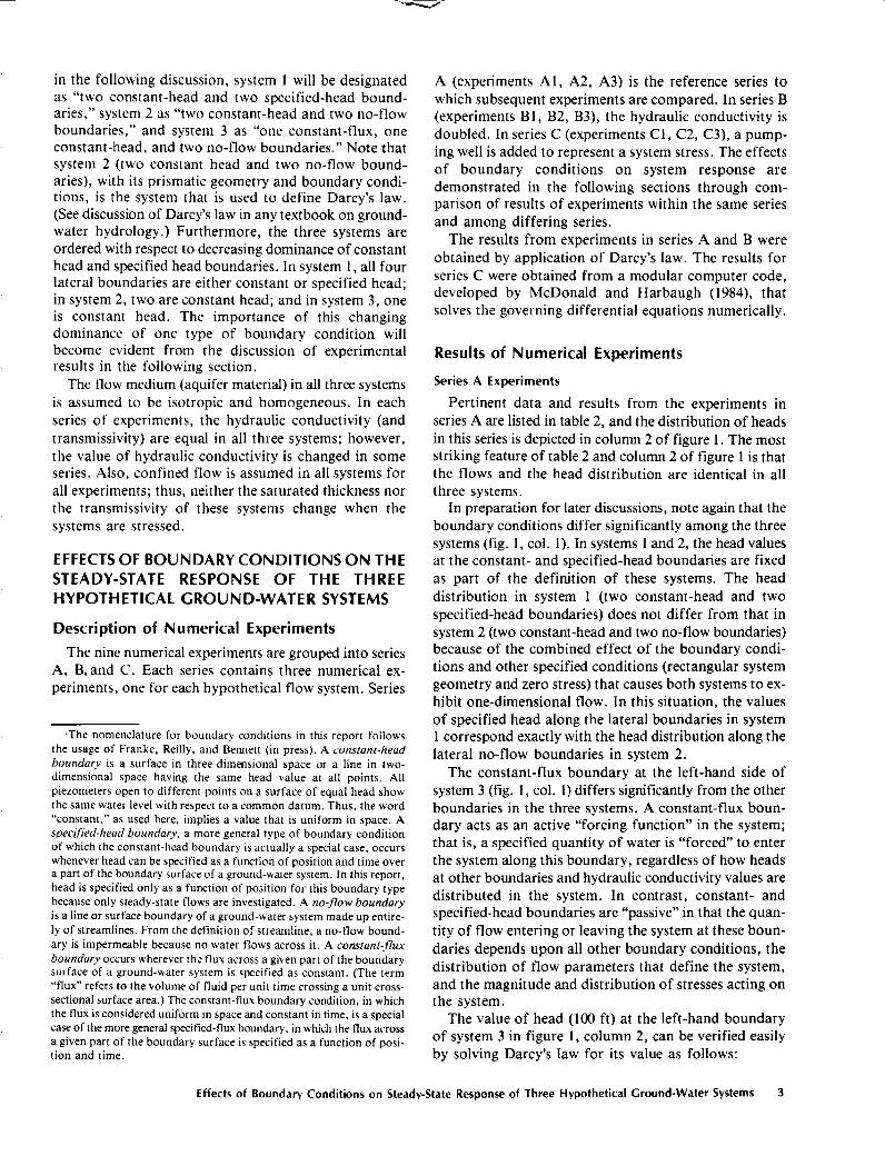
in the following discussion, system 1 will be designatedas "two constant-head and two specified-head bound-aries," system 2 as "two constant-head and two no-flowboundaries," and system 3 as "one constant-flux, oneconstant-head, and two no-flow boundaries." Note thatsystem 2 (two constant head and two no-flow bound-aries), with its prismatic geometry and boundary condi-tions, is the system that is used to define Darcy's law .(See discussion of Darcy's law in any textbook on ground-water hydrology .) Furthermore, the three systems areordered with respect to decreasing dominance of constanthead and specified head boundaries . In system 1, all fourlateral boundaries are either constant or specified head;in system 2, two are constant head ; and in system 3, oneis constant head . The importance of this changingdominance of one type of boundary condition willbecome evident from the discussion of experimentalresults in the following section .The flow medium (aquifer material) in all three systems

is assumed to be isotropic and homogeneous . In eachseries of experiments, the hydraulic conductivity (andtransmissivity) are equal in all three systems ; however,the value of hydraulic conductivity is changed in someseries . Also, confined flow is assumed in all systems forall experiments ; thus, neither the saturated thickness northe transmissivity of these systems change when thesystems are stressed .

EFFECTS OF BOUNDARY CONDITIONS ON THESTEADY-STATE RESPONSE OF THE THREEHYPOTHETICAL GROUND-WATER SYSTEMS

Description of Numerical ExperimentsThe nine numerical experiments are grouped into series

A, B, and C . Each series contains three numerical ex-periments, one for each hypothetical flow system . Series

'The nomenclature for boundary conditions in this report followsthe usage of Franke, Reilly, and Bennett (in press) . A constant-headboundary is a surface in three-dimensional space or a line in two-dimensional space having the same head value at all points . Allpiezometers open to different points on a surface of equal head showthe same water level with respect to a common datum . Thus, the word"constant," as used here, implies a value that is uniform in space . Aspecified-head boundary, a more general type of boundary conditionof which the constant-head boundary is actually a special case, occurswhenever head can be specified as a function of position and time overa part of the boundary surface of a ground-water system . In this report,head is specified only as a function of position for this boundary typebecause only steady-state flows are investigated . A noflow boundaryis a line or surface boundary of a ground-water system made up entire-ly of streamlines . From the definition of streamline, a no-flow bound-ary is impermeable because no water flows across it . A constant-fluxboundary occurs wherever the flux across a given part of the boundarysurface of a ground-water system is specified as constant . (The term"flux" refers to the volume of fluid per unit time crossing a unit cross-sectional surface area .) The constant-flux boundary condition, in whichthe flux is considered uniform in space and constant in time, is a specialcase of the more general specified-flux boundary, in which the flux acrossa given part of the boundary surface is specified as a function of posi-tion and time .

A (experiments Al, A2, A3) is the reference series towhich subsequent experiments are compared. In series B(experiments 131, B2, B3), the hydraulic conductivity isdoubled . In series C (experiments Cl, C2, C3), a pump-ing well is added to represent a system stress . The effectsof boundary conditions on system response aredemonstrated in the following sections through com-parison of results of experiments within the same seriesand among differing series .The results from experiments in series A and B were

obtained by application of Darcy's law . The results forseries C were obtained from a modular computer code,developed by McDonald and Harbaugh (1984), thatsolves the governing differential equations numerically .

Results of Numerical Experiments

Series A Experiments

Pertinent data and results from the experiments inseries A are listed in table 2, and the distribution of headsin this series is depicted in column 2 of figure 1 . The moststriking feature of table 2 and column 2 of figure 1 is thatthe flows and the head distribution are identical in allthree systems .

In preparation for later discussions, note again that theboundary conditions differ significantly among the threesystems (fig . 1, col . 1) . In systems 1 and 2, the head valuesat the constant- and specified-head boundaries are fixedas part of the definition of these systems . The headdistribution in system 1 (two constant-head and twospecified-head boundaries) does not differ from that insystem 2 (two constant-head and two no-flow boundaries)because of the combined effect of the boundary condi-tions and other specified conditions (rectangular systemgeometry and zero stress) that causes both systems to ex-hibit one-dimensional flow . In this situation, the valuesof specified head along the lateral boundaries in system1 correspond exactly with the head distribution along thelateral no-flow boundaries in system 2 .The constant-flux boundary at the left-hand side of

system 3 (fig . 1, col . 1) differs significantly from the otherboundaries in the three systems . A constant-flux boun-dary acts as an active "forcing function" in the system ;that is, a specified quantity of water is "forced" to enterthe system along this boundary, regardless of how headsat other boundaries and hydraulic conductivity values aredistributed in the system . In contrast, constant- andspecified-head boundaries are "passive" in that the quan-tity of flow entering or leaving the system at these boun-daries depends upon all other boundary conditions, thedistribution of flow parameters that define the system,and the magnitude and distribution of stresses acting onthe system .The value of head (100 ft) at the left-hand boundary

of system 3 in figure 1, column 2, can be verified easilyby solving Darcy's law for its value as follows :

Effects of Boundary Conditions on Steady-State Response of Three Hypothetical Ground-Water Systems 3

Constant-fluxboundaryq in =constant

SYSTEM GEOMETRY AND

RESULTS OF SERIES ABOUNDARY CONDITIONS

EXPERIMENTS(Head, in feet)

Constant-

, "

" *

" ' .head

" .Flow domainboundary

. " , , . " .",=constant

Streamline boundary

Streamline boundaryE

(no flow)

F

H

Same as EF

G

Experiment A2

SYSTEM 2

I

(no flow)

J

L Same as IJSYSTEM 3

Constant-headboundaryh2 = constant

Constant-headboundaryh2= constant

Constant-headboundaryh=constant

One-dimensional flow patterns

75 1",50 ~25

Experiment A1

qin=10 ft/day

100I`75 I/0 I/25 Ih=oft

1(ft3/d)/ft 2 ]

Experiment A3

Hydraulic conductivity (K)=2ft/d

0 1

i

i

+ X0 10 20

LENGTH (ft)(1)

(2)

Figure 1 . Boundary conditions and distributions of head in all nine numerical experiments .

Q =KA(h, - hr) ,L

L = distance between the two parallel equipoten-tial surfaces (feet) .

where Q = total discharge or throughflow of system

Solving for h, and substituting appropriate numerical(cubic feet per day),

values, we obtainK = hydraulic conductivity of the earth material in

QL _ 80 ft 3 /d - 20 ftthe prism (feet per day),

h,_KA

2 ft/d " 8 ft'_- 100 ft .

A = cross-sectional area of the prism perpendicularto the direction of flow (square feet),

Results of the series A experiments demonstrate thath l, h,.= heads at the left- and right-hand boundaries

the same potential distributions and flows can be obtained(feet), respectively, and

in steady-state simulations with distinctly different boun-

4


A

Specified-head boundary

hh=ht

-x2-xt ) xy

,

BConstant-head Flow "domain. 'boundary .

ht = constantD Same as AB C

SYSTEM 1

1-11h t = 100 ft

gln=10 ft/day

1(ft 3/d)/ft 2 ]

Figure 1 . Continued .

Series B Experiments

RESULTS OF SERIES BEXPERIMENTS(Head, in feet)

One-dimensional flow patterns

',75 ~50JExperiment B1

Experiment E12

Experiment B3

Hydraulic conductivity (K) = 4ft/d

dary conditions . Furthermore, as stated above, series Aexperiments provide a point of reference for the subse-quent experiments . Comparison of results from theexperiments in series B and C with those from series Aelucidates the effect of the respective boundary conditionson the response of these systems .

Pertinent data on the experiments in series B are listedin table 3, and the head distributions for this series are

1(ft 3/d)/ft 2 ]

RESULTS OF SERIES CEXPERIMENTS(Head, in feet)

Two-dimensional flow patterns

Experiment C 1

Experiment C2

1-111

-5q ;� =10 ft/day

I (110(O(n

f 5l

h2=oft

Experiment C3

Hydraulic conductivity (K) = 2ft/d" Well location

Qwell=100 ft3/d

shown in column 3 of figure 1 . The three systems in seriesB differ from those in series A only in that the hydraulicconductivity in series B has been doubled to 4 ft/d . Acomparison between tables 2 and 3 and between columns2 and 3 in figure 1 reveals several pertinent facts .The quantity of water flowing through systems 1 (two

constant-head and two specified-head boundaries) and2 (two constant-head and two no-flow boundaries) inseries B (160 ft 3/d) is double that in series A (80 ft 3/d) .Simply stated, if the heads in these two systems are the

Effects of Boundary Conditions on Steady-State Response of Three Hypothetical Ground-Water Systems

4-1h2 =0ft

5

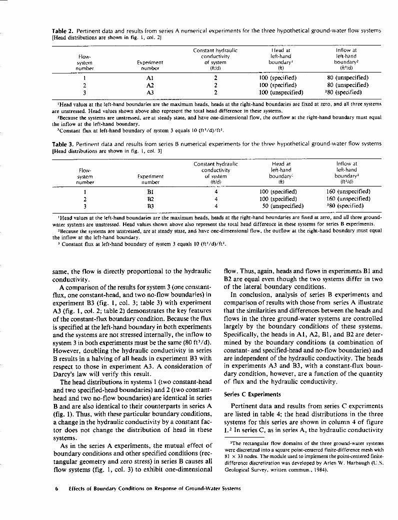
Table 2. Pertinent data and results from series A numerical experiments for the three hypothetical ground-water flow systems[Head distributions are shown in fig . 1, col . 2]

'Head values at the left-hand boundaries are the maximum heads, heads at the right-hand boundaries are fixed at zero, and all three systemsare unstressed. Head values shown above also represent the total head difference in these systems .

=Because the systems are unstressed, are at steady state, and have one-dimensional flow, the outflow at the right-hand boundary must equalthe inflow at the left-hand boundary .

'Constant flux at left-hand boundary of system

6

Table 3. Pertinent data and results from series B numerical experiments for the three hypothetical ground-water flow systems[Head distributions are shown in fig . 1, col . 3]

Flow-system

Experimentnumber

number

1

1312

1323

133

3 equals 10 (ft'/d)/ft' .

same, the flow is directly proportional to the hydraulicconductivity .A comparison of the results for system 3 (one constant-

flux, one constant-head, and two no-flow boundaries) inexperiment B3 (fig . 1, col. 3; table 3) with experimentA3 (fig . 1, col . 2; table 2) demonstrates the key featuresof the constant-flux boundary condition. Because the fluxis specified at the left-hand boundary in both experimentsand the systems are not stressed internally, the inflow tosystem 3 in both experiments must be the same (80 ft 3/d) .However, doubling the hydraulic conductivity in seriesB results in a halving of all heads in experiment B3 withrespect to those in experiment A3 . A consideration ofDarcy's law will verify this result .Thehead distributions in systems 1 (two constant-head

and two specified-head boundaries) and 2 (two constant-head and two no-flow boundaries) are identical in seriesB and are also identical to their counterparts in series A(fig . 1) . Thus, with these particular boundary conditions,a change in the hydraulic conductivity by aconstant fac-tor does not change the distribution of head in thesesystems .As in the series A experiments, the mutual effect of

boundary conditions and other specified conditions (rec-tangular geometry and zero stress) in series B causes allflow systems (fig . 1, col . 3) to exhibit one-dimensional

Constant hydraulicconductivityof system

(ft/d )

444


Series C Experiments

Head at

Inflow atleft-hand

left-handboundary'

boundary'(ft)

(ft3/d)

100 (specified)

160 (unspecified)100 (specified)

160 (unspecified)50 (unspecified)

380 (specified)

'Head values at the left-hand boundaries are the maximum heads, heads at the right-hand boundaries are fixed at zero, and all three ground-water systems are unstressed . Head values shown above also represent the total head difference in these systems for series B experiments .

2Because the systems are unstressed, are at steady state, and have one-dimensional flow, the outflow at the right-hand boundary must equalthe inflow at the left-hand boundary .

' Constant flux at left-hand boundary of system 3 equals 10 (ft'/d)/ftz .

flow . Thus, again, heads and flows in experiments B1 andB2 are equal even though the two systems differ in twoof the lateral boundary conditions .

In conclusion, analysis of series B experiments andcomparison of results with those from series A illustratethat the similarities and differences between the heads andflows in the three ground-water systems are controlledlargely by the boundary conditions of these systems .Specifically, the heads in Al, A2, B1, and B2 are deter-mined by the boundary conditions (a combination ofconstant- and specified-head and no-flow boundaries) andare independent of the hydraulic conductivity . The headsin experiments A3 and B3, with a constant-flux boun-dary condition, however, are a function of the quantityof flux and the hydraulic conductivity .

Pertinent data and results from series C experimentsare listed in table 4 ; the head distributions in the threesystems for this series are shown in column 4 of figure1 . 2 In series C, as in series A, the hydraulic conductivity

2The rectangular flow domains of the three ground-water systemswere discretized into a square point-centered finite-difference mesh with81 x 33 nodes. The module used to implement the point-centered finite-difference discretization was developed by Arlen W . Harbaugh (U .S .Geological Survey, written commun ., 1984) .

Constant hydraulic Head at Inflow atFlow- conductivity left-hand left-handsystem Experiment of system boundary' boundaryznumber number (ft/d) (ft) (ft 3/d)

1 Al 2 100 (specified) 80 (unspecified)2 A2 2 100 (specified) 80 (unspecified)3 A3 2 100 (unspecified) 380 (specified)

Table 4. Pertinent data and results from series C numerical experiments for the three hypothetical ground-water flow systems[Head distributions are shown in fig . 1, cot. 41

equals 2 ft/d in all three systems. The only difference be-tween series AandC is that series C has a centrally placedwell pumping at the rate of 100 ft 3 /d . Thus, the threeground-water systems in series C are subjected to an in-ternal stress .A comparison of the head distributions in the three

systems of series C (fig . 1, cot. 4) reveals severalqualitative facts . First, unlike the head distributions inseries A and B (fig . 1, cots . 2, 3), those in this series dif-fer significantly from one another . Second, as would beexpected in response to a point stress, flow patterns incolumn 4of figure 1 clearly are two dimensional, as evi-denced by the curved potential lines, in contrast to theone-dimensional flow patterns in series A and B. Third,the heads become progressively lower (drawdowns dueto pumping become progressively larger) in the sequencefrom system 1 through system 3 (fig . 1, cot . 4) . This isparticularly significant because it illustrates the effectsof boundary conditions on the response of systems tostress as discussed later in this section .Water budgets were developed for the three ground-

water systems in series C, the results of which are sum-marized in table 5 . In considering these water budgets,recall the unstressed water budget for the three systemsin series A (table 2) :

Inflow at left boundary = Outflow at right boundary= 80 ft 3/d .

In system 1 (two constant-head and two specified-headboundaries) of series C, significant quantities of infloware derived from the lateral specified-head boundaries (95ft'/d) . Inflow from the left-hand boundary has in-creased by only 2 .5 ft 3 /d, and outflow to the right-hand boundary has decreased by 2 .5 ft 3/d .

In system 2 (two constant-head and two no-flow boun-daries), the sources of water to the pumping well are iden-tified readily . Inflow from the left-hand constant-headboundary has increased by 50 ftl/d from 80 ftl/d in theunstressed system in series A to 130 ft 3 /d, and outflowto the right-hand constant-head boundary has decreasedby 50 ftl/d to 30 ft 3/d .

'Maximum head in ground-water system .'Constant head values of zero at right-hand boundaries are head datum in all three ground-water systems .

In system 3 (one constant-flux, one constant-head, andtwo no-flow boundaries) of series C, the only possiblesource of increased recharge to the system is the right-hand constant-head boundary . Thus, the water pumpedfrom the well (100 ft 3/d) is derived from the left-handconstant-flux boundary (80 ft 3/d) and from inducedrecharge at the right-hand constant-head boundary (20ft 3/d). In all three systems, the right-hand boundary isa constant head . Only in experiment C3 is the gradientat the right-hand boundary reversed (fig . 1, cot. 4) .The differing responses of the three ground-water

systems to the stress exerted by the pumping well in seriesC are related clearly to the boundary conditions, and thisbecomes obvious when we recall that the heads and flowsin the three systems were identical in series A, where thesystems were unstressed (fig . l, cot. 2; table 2) . A com-parison of water budgets and head distributions in seriesA with those in series C illustrates the effects of differenttypes of boundary conditions when the system is stressed .Investigating the stressed systems by superposition, asdiscussed in Appendix 2, reveals the role of the variousboundaries as sources of water to the pumping well evenmore clearly.The importance of the constant- and specified-head

boundaries as sources of water in series C experimentsis indicated by the total flow of water through the threesystems (table 5) . In system 1, with two constant- andtwo specified-head boundaries, the total flow (inflow oroutflow) is 177.5 ft 3 /d ; in system 2, with two constant-head boundaries, total flow is 130 ft 3/d; and, in system3, with one constant-head boundary (and one constant-flux boundary), total flow is 100 ft'/d . Furthermore,comparison of the head distributions in the three systems(fig . 1, cot. 4) indicates that the closer the constant- orthe specified-head boundaries are to the pumping well,the more effectively these boundaries will maintain heads.The previous discussion demonstrates the control ex-

ercised by constant- and specified-head boundaries on theheads and flows in the three systems. An importantcharacteristic of simulated constant-head boundaries isthat they are capable of providing any quantity of water

Effects of Boundary Conditions on Steady-State Response of Three Hypothetical Ground-Water Systems 7

Approximate head atpumping well

Flow-system Experiment Constant hydraulic Head at Discharge (pumping node innumber number conductivity of left-hand of pumping numerical

system boundary' well, Q simulation)'(ft/d) (ft) (ft 3 /d) (ft)

1 Cl 2 100 (specified) 100 132 C2 2 100 (specified) 100 -73 C3 2 38 (approximate) 100 -38

(unspecified)

Table 5 . Water budgets' for series C experiments[Boundary conditions and heads are shown in fig . 1 . All flows are in cubic feet per day]

' Inflow components are designated arbitrarily as positive, and outflow components, as negative (-) . Thus, to maintain continuity, the algebraicsum of the entries in any row must equal zero .

2 Constant flux at left-hand boundary of system 3 equals 10 (ft'/d)/ft' .

that is required, even though the heads in the aquifer mustdecrease and the gradients to the well must increase asmore water is pumped from the well . In real ground-watersystems, the physical limit on drawdown at the pumpingwell imposes a constraint on pumpage . This physical con-straint, however, does not exist in numerical ormathematical simulations of systems .

IMPLICATIONS OF NUMERICAL EXPERIMENTSFOR SIMULATION OF GROUND-WATERSYSTEMS

This discussion relates the results of the experimentsdepicted in figure 1 to the simulation of ground-watersystems . (The significance of the mathematical formula-tion of the experiments is discussed in Appendix 1) . Thesimplified geometry of the three flow systems helps toverify the observations and conclusions herein but doesnot restrict their validity .One of the key elements in describing or defining a

ground-water system, and probably the one most subjectto error, is the specification of appropriate boundary con-ditions . The boundary conditions for the three systemsused as examples in this study differ significantly (fig .1, col . 1) . The heads in system 1 are the most constrained,in that the four lateral boundaries are either constant heador specified head. Heads in system 2 are constrained bytwo lateral constant-head boundaries (the left- and right-hand boundaries) . The heads in system 3 are the least con-strained in that the system has only one constant-headboundary. Systems 1 and 2 are similar in that all bound-ary conditions are constant head, specified head, or noflow . System 3 differs from systems 1 and 2 in that it hasone constant-flux boundary . The observed differences insystem response in figure 1, resulting primarily fromvariations in boundary conditions, suggest importantgeneral implications for system simulation that arediscussed further in the following sections .

Model Calibration

The process of simulating natural ground-watersystems often includes a steady-state "calibration" of the

8 Effects of Boundary Conditions on Response of Ground-Water Systems

unstressed system, which involves a continuing com-parison of model heads and flows with correspondingfield measurements from the unstressed natural system,followed by adjustments in the model if these com-parisons are not sufficiently close . Hydraulic parameters(hydraulic conductivity and transmissivity) are adjustedroutinely in the calibration process . In most modelstudies, however, adjustments during calibration do notinvolve changes in boundary conditions . In series A ex-periments, the heads and flows in all three systems areidentical (table 2) despite the significant differences inboundary conditions . This suggests that the effect ofboundary conditions on system response should be con-sidered at every phase of an investigation involvingsimulation, including the calibration phase, and that theprocess of calibration might include sensitivity analyseson arbitrarily selected boundary conditions to verify thevalidity of the selected boundary types .The role of boundary conditions in the calibration

process is illustrated by the results of series B experiments(fig . 1, col . 3 ; table 3) . The heads in systems 1 and 2 arefixed, and the flow through the system is dependent onthe hydraulic conductivity . Thus, the heads in ex-periments Al, A2, B1, and B2 (fig . 1 ; tables 2, 3) remainthe same, and the flows change in proportion to thehydraulic conductivity . In experiment 133, however, theflow is specified, and the heads in the system adjust ac-cording to the quantity of flow and the distribution ofhydraulic conductivity . Thus, comparison of results ofexperiments A3 and 133 shows that the flow stays thesame, whereas the heads change inversely with thehydraulic conductivity .

Implications of these observations for the process ofcalibration are as follows :

1 .

Heads in systems that are bounded predominantlyby constant- and specified-head boundary condi-tions are insensitive to changes in hydraulic con-ductivity .

2 .

Comparison of measurements or estimates of flowin the natural ground-water system with cor-responding simulated flows is just as critically important in the calibration process as the com-parison of observed heads with simulated heads .

Flow-systemnumber

Experimentnumber

Inflow fromleft-handboundary

Inflow fromlateral

boundaries

Inflow fromright-handboundary

Outflowfrom well

Outflow toright-handboundary

1 Cl 82 .5 (unspecified) 95 (unspecified) 0 -100 -77.52 C2 130 (unspecified) 0 0 -100 -303 C3 280 (specified) 0 20 -100 0

Solute Transport Analysis

The two immediately preceding observations also arerelevant to ground-water solute transport simulation .Simulation of solute transport involves coupling aground-water flow model that calculates the spatialdistribution of ground-water velocities and a transportmodel that calculates changes in the concentration ofsolute as a function of space and time . Because transportanalysis involves a very local area of interest, one com-mon approach to solute transport simulation in twodimensions is to bound the local flow system containingthe contaminant plume with specified head boundaries,to calculate ground-water heads within the area surround-ed by the specified heads with the flow model, and todetermine a velocity distribution based on these calculatedheads.'

Because the heads calculated in this approach are con-strained by the nearby specified-head boundaries, theyusually compare well with observed heads in the realsystem . This approach, however, does not allow possiblylarge local variations in hydraulic conductivity andcoupled variations in local fluxes in the real system tobe accounted for in the calculation of the simulated headsin the neighborhood of the contaminant plume becausesystems constrained in this manner (for example, ex-periments Al, A2, B l, and 132) are insensitive to hydraulicconductivity; that is, any hydraulic conductivity valuegives almost the same head distribution . Thus, this ap-proach results in possibly large errors in simulated fluxesin the neighborhood of the contaminant plume, which,in turn, cause large errors in the calculated velocitydistribution .

In conclusion, an extension of point 2 in the previoussection, "Model Calibration," applies to transportanalysis . To insure that simulated ground-water velocitiescorrespond closely to velocities in the real system,simulated flows (in addition to simulated heads) must cor-respond to those occurring in the real system .

Effects of Stress Magnitude

A comparison of series C results with those from seriesA and B demonstrates one of the most important pointsin this discussion-that the differences between the ef-fect of different boundary conditions on system responsebecome greater when the system is under stress and in-crease with increasing stress ; for example, the stress inseries C (100 ft'/d) is relatively large compared to the flowthrough the unstressed series A and B systems (80 ft'

'The value of ground-water velocity at a point is the product of thehydraulic conductivity and hydraulic gradient at the point divided bythe average porosity of the earth material in the neighborhood of thepoint .

/d,)°, and the head distributions and flows in series C ex-periments differ significantly from one another (fig . 1,col . 4 ; tables 4, 5) . Furthermore, because the heads insystems C1, C2, and C3 are progressively less constrainedby constant- and specified-head boundaries, they declinefrom experiment Cl through C3 .

If the effects of different boundary conditions in other-wise similar systems become more evident as the stressis increased, then the effects of the stress in series C ex-periments, which is large with respect to flows in theunstressed system, should become less pronounced as thestress is decreased . To verify this point, stresses equaling1 and 10 ft'/d, in addition to 100 ft'/d, were applied tothe three ground-water systems in series C .The drawdowns for these stresses are summarized in

table 6, wherein it is assumed that the maximumdrawdowns in the stressed systems occur at the pumpingwell (pumping node in the numerical simulation) . Thedrawdown at the pumping well for a stress of 100 ft'/dcan be calculated by subtracting the head at the pump-ing well (table 4) from the original unstressed head at thatlocation, which is 50 ft ; for example, in experiment Cl,the drawdown at the pumping well equals 50 ft minus13 ft, or 37 ft . s Because the three hypothetical ground-water systems are confined and, therefore, linear systems(exhibit a linear relation between system stress and systemresponse), the drawdowns listed in table 6 are directly pro-portional to the system stress relative to the knowndrawdowns for a stress of 100 ft'/d .

Table 6. Drawdowns resulting from three selected well-discharge rates at the pumping well in the three ground-waterflow systems

Well discharge(ft ,ld)

Drawdown(ft)

Flow system

Flow system

Flow system1

2

3

1

0.37 0.57 0.88

10

3.7

5.7

8.8100 37

57

88

The data in table 6 indicate that for a stress of 1 ft'/d,the drawdowns everywhere in all three hypotheticalground-water systems are less than 1 ft . With the 10-ftcontour interval used for these hypothetical systems(similar to contour intervals used in potentiometric mapsof natural systems) and considering the natural small-scale background fluctuations in water levels ("noise") andpaucity of water-level data that probably would be en-countered if these systems were natural systems, water-

'The magnitude of a local stress is usually small relative to the totalwater budget for a regional or subregional ground-water system .'Drawdown data at the pumping well also can be obtained directly

from table A-2.1 in Appendix 2 .

Implications of Numerical Experiments for Simulation of Ground-Water Systems 9

level maps of the three systems can be regarded as vir-tually indistinguishable when a stress of 1 ftl/d is im-posed . However, the source of water to the pumping wellstill differs significantly among the three systems, and thepercentage of total water that is derived from each bound-ary is the same as the percentage for a stress of 100 ftl/d(or any other pumping rate at this location) and can becalculated easily from the data in table 5 by assuming alinear relation between pumping rate and boundary flows .

Potentiometric maps of the three hypothetical ground-water systems at a well discharge of 10 ftl/d are shown

1 0

Constant-head ~+boundaryh t = constant

Constant-flux ~+boundaryq in =constant

SYSTEM GEOMETRY ANDBOUNDARY CONDITIONS

" " Flow domain

TTI7T7/777-77H

Same as EF

G

SYSTEM 2

Streamline boundaryI

(no flow)

J

Same as IJL

Y

SYSTEM 3

8+

03 0

I-~ x0 10 20

LENGTH (ft)

Constant-headboundaryh 2 = constant

Constant-headboundaryh2 = constant

Constant-,, head

boundaryh= constant


in figure 2 . At this level of stress and a contour intervalof 10 ft, differences in head among the three systems arebarely discernible . The maps for system 1 (two constant-head and two specified-head boundaries) and system 2(two constant-head and two no-flow boundaries) arebarely distinguishable from one another and do not dif-fer significantly from maps of the unstressed systems (fig .1, col . 2) . As might be expected from previous discus-sion of the three systems, the water-level contours insystem 3 (one constant-flux, one constant-head, and twono-flow boundaries) show the greatest deviation from

qin =10 ft/day

1(f t 3/d)/ft 2 I

RESULTS OF EXPERIMENTS(Head, in feet)

Hydraulic conductivity (K) = 2ft/d" Well location

Q"'11= 10 ft3/d

h=Oft

Figure 2 . Distribution of head in a series of experiments in which hydraulic conductivity is a constant of 2 ft/d and the systemis stressed by a centrally placed well discharging at a rate of 10 ft3/d .

Specified-head boundary

h=h_~

hi _h 2 ) xA 1 x2-xt B

Constant-head Flow "domain . "boundaryh t = constant

~

CD Same as AB

SYSTEM 1

Streamline boundaryE (no flow) F

unstressed water levels, particularly in the left-hand partof the system near the constant-flux boundary . However,these differences probably would be much less apparentand more difficult to interpret if these maps were beingcompared to a potentiometric map from a "noisy" andmore complex natural system .Comparison of the three pumpage stresses (1, 10, and

100 ft 3 /d) with their associated water-level maps il-lustrates a basic tenet of ground-water systems simu-lation-that the ability of ground-water models to predictthe response of natural systems to stress generally dependson the magnitude of that stress ; for example, suppose thatone of the hypothetical ground-water systems correspondsto the natural system under study and that the boundaryconditions of this system are, in part, unknown or uncer-tain . Model calibration to measured water levels resultingfrom a pumping stress of 1 ft 3 /d easily could producea close match between simulated and measured waterlevels even if the boundary conditions used in the modelbore little resemblance to those in the natural system .Whetherthis model, when calibrated at a stress of 1 ft 3/d,would predict correctly the natural system in responseto a stress of 10 or 100 ft 3 /d would depend in largemeasure on how well the boundary conditions in themodel correspond to those in the natural system .

In conclusion, one reason why the ability of ground-water models to predict natural system response is stressdependent is that specification of boundary conditionsis uncertain . Thus, the predictive capability of a modelis most reliable when the stress to be simulated is notsignificantly greater than the stress already observed inthe natural system and used in model calibration .The concepts presented herein suggest that, during all

phases of a ground-water investigation, the hydrologist'sconcept of the natural system must be reconsidered con-tinually and the physical characteristics of the variouspostulated boundary conditions must be related con-tinually to the evolving concept of the natural system .Furthermore, an analysis of historical stress-response datacan improve the selection of boundary conditions as wellas other aspects of ground-water simulation throughmathematical-numerical models .

SUMMARY AND CONCLUSIONS

The most critical aspect in describing or definingground-water systems for purposes of simulation is thespecification of appropriate boundary conditions ; this isthe aspect most subject to error . The goal of simulationis to represent the physical system in its essential featuresas a mathematical-numerical or other appropriate typeof model . Essential features include hydraulic character-istics related to the occurrence and movement of groundwater at the boundaries of the natural ground-watersystem that is isolated for study . Boundary conditions

determine the hydraulic characteristics of the system atits boundaries; correct specification of boundary condi-tions in a model means that the boundary conditions inthe model correspond sufficiently to those in the naturalsystem to ensure that the response of model and naturalsystem to the same hydraulic stress will match acceptably .A series of numerical experiments on three hypothetical

ground-water systems is used to illustrate this criticalnature of boundary conditions . These three hypotheticalground-water systems are rectangular sand prisms withthe same dimensions but with different combinations ofconstant-head, specified-head, no-flow, and constant-fluxboundary conditions . In the first series of numerical ex-periments, the heads and flows in all three systems areidentical, as are the hydraulic conductivity and systemgeometry . However, when the systems are subjected toan equal stress by a pumping well in the third series, eachdiffers significantly in its response . The highest heads(smallest drawdowns) and flows occur in the systems mostconstrained by constant- or specified-head boundaries.These and other results indicate that -1 . The principal observation concerning the results of the

numerical experiments on the three hypotheticalground-water systems that are the same in allrespects except their boundary conditions is thatthese three systems did in fact respond very dif-ferently to an imposed stress . This observationunderscores the fact that differing boundary con-ditions define different ground-water systems, evenif the geometry and hydraulic conductivity of thesystems are identical . Stating the same idea from aslightly different viewpoint-if a simulated ground-water system has incorrect boundary conditions(conditions that do not correspond to those in thenatural system under study), then the simulation ex-ercise is solving the wrong problem and, by defini-tion, will provide the wrong solution .

2 . A close match between the head distribution in amodel and that in the natural system does notguarantee that the two systems correspond in theirphysical and hydraulic features nor in their bound-ary conditions . Model calibration with respect toheads alone is not reliable for unstressed steady-stateanalyses but tends to improve in stressed systemsand usually becomes increasingly reliable as thestress increases . In stressed and unstressed systems,however, correct boundary conditions are essentialto the representation of sources of water and pat-terns of flow within the system . This is illustratedclearly by the water budgets for the three stressedsystems (series C experiments), in which the percen-tage of water to the pumping well from the majorsources differed significantly as a result of the dif-fering boundary conditions in the systems . Thus, in-corporating measurements and estimates of ground-water flow from the natural system in the process

Summary and Conclusions

1 1

of model development and assessment of its accept-ability (the calibration process) is of utmostimportance .

3 . The effects of boundary conditions on system responseshould be considered at every phase of an investiga-

tion involving simulation, including the calibrationphase, which should include sensitivity analyses onarbitrarily selected boundary conditions .

In conclusion, the boundary conditions that areselected for simulation of a ground-water system arecritical to the success of a ground-water systems analysis .They deserve continual reevaluation and modification asinvestigation proceeds and new information and under-standing are acquired .

12 Effects of Boundary Conditions on Response of Ground-Water Systems

REFERENCES CITED

Bear, Jacob, 1979, Hydraulics of groundwater: New York,McGraw-Hill, 567 p.

Franke, O . L., Reilly, T. E., and Bennett, G. D., in press ,Definition of boundary and initial conditions in the analysisof saturated ground-water flow systems-An introduction:U.S . Geological Survey Techniques of Water Resources In-vestigations, Book 3, Chapter B5 .

McDonald, M. G., and Harbaugh, A. W., 1984, A modularthree-dimensional finite-difference ground-water flowmodel: U.S . Geological Survey Open-File Report 83-875,528 p .

Reilly, T. E ., Franke, O. L., and Bennett, G. D., in press ,The principle of superposition and its application inground-water hydraulics : U .S . Geological Survey Techniques of Water Resources Investigations, Book 3, ChapterB6.

APPENDIXES

APPENDIX 1 . Comparison of the Governing Differential Equations and Boundary Conditions ThatApply to the Three Hypothetical Ground-Water Systems Analyzed in this Report

This appendix takes a small additional step in relating thesystem responses (potential distributions and flows), which areillustrated by the nine experiments discussed in the main text,to the governing differential equations and boundary conditions .All three ground-water systems analyzed in this report areassumed to be two dimensional, and all nine numerical examplesare steady state . A general and often-used ground-water flowequation for two-dimensional, steady-state problems is

axT, ax ) + ay (TY-ay-) +W(x,Y)=0,

(A1)

where T, TY =transmissivity values in the x and y directions(square feet per day), respectively, and

W=an areal input or withdrawal of water per unittime (feet per day) .

As written, T and W can be varied as a function of location(x, Y)-

In the three systems under discussion, Tx and TY areconstant and equal; that is, the flow domains are assumed to beisotropic and homogeneous with respect to transmissivity . Thus,equation Al can be simplified further to

The ground-water flow equations and boundary conditions thatapply to the nine numerical experiments depicted in figure 1,are listed in table A-1 .1 and are expressed in formalmathematical notation.Only two different governing equations are given in table

A-1 .1,

Series A and B Experiments

_a 2h a2h Waxe + aye + T(x,Y) =0.

(A2)

which is the same as equation A2 .

Because all six experiments in series A and B use the samegoverning differential equation (table A-1 .1), it is necessary to

look beyond the equations in comparing these experiments andto consider the boundary conditions to explain the differencein response between system 3 and systems 1 and 2. The key fac-tor pertains to what is specified in the governing equations andboundary conditions . Examination of the governing differen-tial equation (eq A3) and the boundary conditions for systems1 and 2 in series Aand B reveals that the hydraulic conductiv-ity or transmissivity does not enter into the mathematical for-mulation of these four problems . Thus, any constant value ofhydraulic conductivity in an isotropic and homogeneous systemwill give the same head (or potential) distribution . In otherwords, the head distribution in these four problems is indepen-dent of the transmitting properties of the porous medium andis determined entirely by the boundary conditions . This is thereason for the previous observation that the head distributionremained unchanged in the experiments for systems 1 and 2 inseries A and B . In contrast, the specified-flux boundary condi-tion for the left-hand side of system 3 contains the hydraulicconductivity . Thus, the head (or potential) distribution in thissystem is dependent on the transmitting properties of themedium, as was shown in the numerical results for experimentsA3 and B3 .

Series C Experiments

In series C experiments, a local stress is given as part of theproblem definition . In these experiments, the dependence of thehead distribution on the value of the transmissivity that is as-signed can be easily inferred because Tappears explicitly in thegoverning equations.The reason for this comparison of the mathematical formula-

tions for the experiments described herein is to emphasize theimportance of boundary conditions in problem definition . Inseries A and B, the head distributions for systems 1 and 2 aredetermined entirely by the boundary conditions and are indepen-dent of the medium transmitting properties . In series C ex-periments (fig . 1, col. 4), the head response of the three systemsand the source of water to the pumping well differ greatly eventhough the governing differential equations are identical.

Appendix 1

15

2 2

X+aYh =0, (A3)

which is known as the Laplace equation, and

_a 2h a2h W=axe + aye +T(x,Y) 0, (A4)

Table A-1 .1 . Governing differential equations and boundary conditions that apply to the hypothetical ground-water systems

in the three series of numerical experiments depicted in figure 1

Flow-systemnumber

Series A and B'

Series C

l

Governing equation :

z zaX +ay=°

ax=+ay+-(x,y)=0

z z z zaxz+aye=0

a +a+T(x ,y) =O

Boundary conditions

h(20,y)= 0

ah(x,8) = 0

1 6


Governing equation :

Boundary conditions :ah

-_Qin

(Same as A and B series)ax

0y)

K

'Boundary conditions in the six experiments in series A and B are expressed in two dimensions (x,y); therefore, the corresponding differential

equations also must be expressed in two dimensions . However, the flow patterns in these examples are one dimensional (fig . 1) because of

the rectangular geometry and lack of internal sources or sinks .

Boundary conditions :h(O,y) =100h(20,y) = 0h(x,0) = 100-5(x)h(x,8) =100-5(x)

Boundary conditions :(Same as A and B series)

2 Governing equation : Governing equation :a z h + azh

=0 z 2

axz ay'ax= + ay=

+-(x,y) = 0

Boundary conditions : Boundary conditions :h(O,y) =100 (Same as A and B series)h(20,y) = 0

x,0)=0y

A(x,8) = 0

3 Governing equation : Governing equation :

APPENDIX 2 . Application of the Principle of Superposition as an Aid in Analyzing the RelationBetween Boundary Conditions and the Response of the Three Ground-WaterSystems to Stress

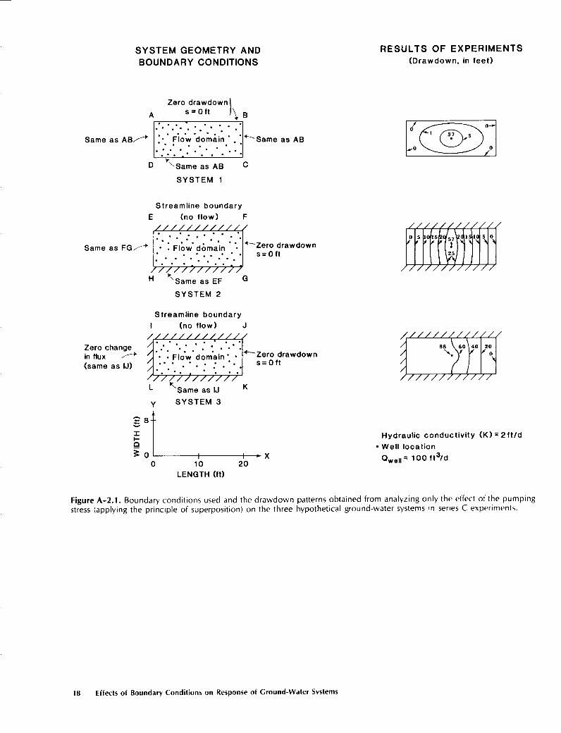
This appendix describes the application of the principle ofsuperposition in the analysis of the response of the three ground-water systems to stress in series C experiments and demonstratesthe conceptual as well as the quantitative value of analyzingthe relation between an imposed stress and the boundary con-ditions of the system in terms of superposition . The principleof superposition is defined and discussed in detail by Reilly,Franke, and Bennett (in press) .The boundary conditions used and the drawdown patterns

obtained by applying superposition to analyze only the effectof the pumping stress on the three systems in series C (fig . 1,cot. 4) are depicted in figure A-2.1 . In addition, water budgetsfor the three stressed systems in which the response to stressis analyzed by superposition are summarized in table A-2.1 .Compare figure A-2.1 and table A-2.1 with column 4 of

figure 1 and tables 4 and 5, which give information on the threestressed ground-water systems in terms of absolute heads. Whensuperposition is applied to system 1 to analyze the effect of thecentrally placed well pumping at the rate of 100 ft'/d (fig .A-2.1), the four lateral boundary conditions are all constantdrawdown (s) with s = 0. Thus, all four boundaries will con-tribute some water to the well discharge. However, because ofthe proximity of the two longest lateral boundaries to the well,it is reasonable to assume that most of the well discharge willbe obtained from them.The entries in table A-2.1 do indicate that for system 1 the

inflows from the left- and right-hand boundaries (2 .5 ft'/d) dueto the pumping well are small relative to the contributions ofthe two lateral boundaries (95 ft'/d) . By definition of super-position, if the drawdowws in figure A-2.1 for system 1 (or anyother system) are subtracted from the heads in the unstressedsystem (fig . 1, cot . 2), the result must be the distribution of ab-solute heads in column 4 of figure 1 ; for example, in system1, the absolute head at the location of the pumping well in the

unstressed system (fig . 1, cot. 2) is 50 ft, the drawdown at thepumping well in figure A-2.1 is about 37 ft, and the absolutehead at the pumping well in column 4 of figure 1 is about 13 ft .

In system 2, the two possible sources of water to the pump-ing well are the left- and right-hand constant-head boundariesat which the drawdown (s) equals zero (fig . A-2 .1) . In this sim-ple, symmetric system, we know without results from anumerical model that one-half of the well discharge (50 ft'/d)must be derived from each boundary (table A-2.1) . This in-flow of 50 ft'/d at the two constant-head boundaries in super-position represents 50 ft'/d of increased inflow at the left-handboundary and 50 ft'/d of decreased outflow at the right-handboundary in the absolute-head system (fig . 1, cot. 4) . Thus, ina water budget for the absolute head system (table 5), the in-flow at the left-hand boundary equals 80 ft'/d plus 50 ft'/dfor a total of 130 ft'/d, and the outflow at the right-hand bound-ary equals 80 ft'/d minus 50 ft'/d for a total of 30 ft'/d.

In system 3, the only possible source for the discharge of thepumping well in superposition is inflow from the right-handconstant-head boundary at which drawdown (s) equals zero (fig .A-2.1 ; table A-2 .1) . This inflow, based on superposition,represents decreased outflow to the right-hand boundary in theabsolute-head system . Thus, in the absolute-head system, theoriginal outflow of 80 ft'/d at the right-hand boundary is re-duced by 100 ft'/d, which results in a net inflow at this bound-ary of 20 ft'/d (table 5) .The advantages of using superposition to analyze systems

undergoing stress are discussed in detail by Reilly, Franke, andBennett (in press) . The principle of superposition can be ex-tremely valuable in the conceptual as well as quantitative con-sideration of how a system reacts to stress or, more specifical-ly, how the boundary conditions ultimately determine the wayin which the system will react to stress .

Appendix 2

1 7

Same as ABA

Same as FGA

Zero changein flux(same as IJ)

SYSTEM GEOMETRY AND

RESULTS OF EXPERIMENTS

BOUNDARY CONDITIONS

(Drawdown, in feet)

8

Zero drawdown'A s=Oft J

D

Flow domain ."

kSame as AB

SYSTEM 1

Streamline boundary

E (no flow) F////////////

" " Flow domain

~Same as AB

C

H

Same as EF

G

SYSTEM 2

Streamline boundary

1

(no flow)

J

~Zero drawdowns= 0ft

Zero drawdowns=Oft

18


111i[A411ill

Hydraulic conductivity (K) = 2ft/d

" Well location3

0 0

10

20

X

Qwe11 = 100 ft3/d

LENGTH (ft)

Figure A-2.1 . Boundary conditions used and the drawdown patterns obtained from analyzing only the effect of the pumping

stress (applying the principle of superposition) on the three hypothetical ground-water systems in series C experiments.

Table A-2.1 . Drawdowns at pumping well and water budgets' for the three hypothetical ground-water flow systems in seriesC experiments (fig . A-2 .1) utilizing the principle of superposition

'By using the principle of superposition, the sum of the inflows from boundaries must equal the discharge of the pumping well, which in theseexamples is 100 ft ;/d .

Appendix 2

19

Drawdown at Inflows (ft 3/d)Flow- pumping wellsystem Experiment (pumping node in Left-hand Two lateral Right-handnumber number numerical simulation) boundary boundaries boundary

(ft)

1 Cl. 37 2.5 95 2.52 C2 57 50 0 503 C3 88 0 0 100

click here to return to usgs publications · principle of superposition 19 metric conversion...

Documents