classification of non-alcoholic beer based on aftertaste sensory

Expert Systems with Applications 39 (2012) 4315–4327

Contents lists available at SciVerse ScienceDirect

Expert Systems with Applications

journal homepage: www.elsevier .com/locate /eswa

Classification of non-alcoholic beer based on aftertaste sensory evaluationby chemometric tools

Mahdi Ghasemi-Varnamkhasti a,b,⇑, Seyed Saeid Mohtasebi a, Maria Luz Rodriguez-Mendez b,Jesus Lozano c, Seyed Hadi Razavi d, Hojat Ahmadi a, Constantin Apetrei e

a Department of Agricultural Machinery Engineering, Faculty of Agricultural Engineering & Technology, University of Tehran, Karaj, Iranb Department of Inorganic Chemistry, E.T.S. Ingenieros Industriales, University of Valladolid, P� del Cauce s/n, 47011 Valladolid, Spainc Grupo de Investigación en Sistemas Sensoriales, Universidad de Extremadura, Av. Elvas s/n, 06006 Badajoz, Spaind Department of Food Science and Engineering, Faculty of Agricultural Engineering & Technology, University of Tehran, Karaj, Irane Department of Chemistry, Physics and Environment, Faculty of Sciences and Environment, ‘‘Dunarea de Jos’’ University of Galat�i, Romania

a r t i c l e i n f o a b s t r a c t

Keywords:Non-alcoholic beerSensory panelArtificial neural networkChemometrics Food quality

0957-4174/$ - see front matter � 2011 Elsevier Ltd. Adoi:10.1016/j.eswa.2011.09.101

⇑ Corresponding author at: Department of AgricultFaculty of Agricultural Engineering & Technology,Box 4111, Karaj 31587-77871, Iran. Tel.: +98 2612801

E-mail addresses: [email protected], [email protected] (M. Ghasemi-Varnamkhasti).

Sensory evaluation is the application of knowledge and skills derived from several different scientific andtechnical disciplines, physiology, chemistry, mathematics and statistics, human behavior, and knowledgeabout product preparation practices. This research was aimed to evaluate aftertaste sensory attributes ofcommercial non-alcoholic beer brands (P1, P2, P3, P4, P5, P6, P7) by several chemometric tools. Theseattributes were bitter, sour, sweet, fruity, liquorice, artificial, body, intensity and duration. The resultsshowed that the data are in a good consistency. Therefore, the brands were statistically classified in sev-eral categories. Linear techniques as Principal Component Analysis (PCA) and Linear Discriminant Anal-ysis (LDA) were performed over the data that revealed all types of beer are well separated except a partialoverlapping between zones corresponding to P4, P6 and P7. In this research, for the confirmation of thegroups observed in PCA and in order to calculate the errors in calibration and in validation, PLS-DA tech-nique was used. Based on the quantitative data of PLS-DA, the classification accuracy values were rankedwithin 49-86%. Moreover, it was found that the classification accuracy of LDA was much better than PCA.It shows that this trained sensory panel can discriminate among the samples except an overlappingbetween two types of beer. Also, two types of artificial networks were used: Probabilistic Neural Net-works (PNN) with Radial Basis Functions (RBF) and FeedForward Networks with Back Propagation (BP)learning method. The highest classification success rate (correct predicted number over total numberof measurements) of about 97% was obtained for RBF followed by 94% for BP. The results obtained in thisstudy could be used as a reference for electronic nose and electronic tongue in beer quality control.

� 2011 Elsevier Ltd. All rights reserved.

1. Introduction

The evaluation is a process that analyzes elements to achievedifferent objectives such as quality inspection, design, marketingexploitation and other fields in industrial companies. In many ofthese fields the items, products, designs, etc., are evaluated accord-ing to the knowledge acquired via human senses (sight, taste,touch, smell and hearing), in such cases, the process is calledsensory evaluation. In this type of evaluation process, an importantproblem arises as it is the modeling and management of uncertainknowledge, because the information acquired by our senses

ll rights reserved.

ural Machinery Engineering,University of Tehran, P.O.

011; fax: +98 0261 [email protected], ghasemi

throughout human perceptions involves uncertainty, vaguenessand imprecision. Sensory evaluation is a scientific discipline usedto evoke measure, analyze and interpret reactions to those charac-teristics of foods and materials as they are perceived by the sensesof sight, smell, taste, touch and hearing. This definition representsan obvious attempt to be as inclusive as is possible within theframework of food evaluation.

As the definition implies, sensory evaluation involves the mea-surement and evaluation of the sensory properties of foods andother materials. Sensory evaluation also involves the analysis andthe interpretation of the responses by the sensory professional;that is, that individual who provides the connection between theinternal world of technology and product development and theexternal world of the marketplace, within the constraints of aproduct marketing brief. This connection is essential such thatthe processing and development specialists can anticipate the im-pact of product changes in the marketplace (Haseleu, Intelmann, &

http://dx.doi.org/10.1016/j.eswa.2011.09.101

mailto:[email protected]

mailto:[email protected]

mailto:ghasemi @eis.uva.es

mailto:ghasemi @eis.uva.es

http://dx.doi.org/10.1016/j.eswa.2011.09.101

http://www.sciencedirect.com/science/journal/09574174

http://www.elsevier.com/locate/eswa

4316 M. Ghasemi-Varnamkhasti et al. / Expert Systems with Applications 39 (2012) 4315–4327

Hofmann, 2009; Yin & Ding, 2009). Similarly, the marketing andbrand specialists must be confident that the sensory propertiesare consistent with the intended target and with the communica-tion delivered to that market through advertising. They also mustbe confident that there are no sensory deficiencies that lead to amarket failure.

Although the brewing of beer has a history extending backsome 800 decades, it is only in the past 150 years that the under-lying science has been substantially unraveled (Bamforth, 2000).Brewing and aging of beer are complex processes during whichseveral parameters have to be controlled to ensure a reproduciblequality of the finished product (Rudnitskaya et al., 2009; Arrieta,Rodriguez-Mendez, de Saja, Blanco, & Nimubona, 2010). These in-clude chemical parameters that are measured instrumentally andtaste and aroma properties that are evaluated by the sensory pan-els. Sensory quality and its measurement are complex issues whichhave received a large amount of attention in the sensory literature.

Brands of non-alcoholic beer are presently being marketed andsold. It is typical that a non-alcoholic beer has a restricted finalalcohol by volume content lower than 0.5% (Porretta & Donadini,2008). Non-alcoholic beers can offer several opportunities thatcan be exploited by marketers. This is true especially in a contextwhere more strict regulations are likely to ban or restrict alcoholicproducts from classical usage situations. This is the case of whereinadministrators are enforcing a renewed battle against alcohol mis-use and abuse. A list of positivities for a beer with a zero alcohollevel is summarized as follows: (a) no restriction for sale by hoursand by places of consumption; (b) no warning on labels for sensi-tive consumer subgroups such as pregnant women; (c) health ben-efits of beer can be promoted; (d) no social judgment in the case ofheavy drinking out of the home; (e) no excise duty or a reducedone is charged (Porretta & Donadini, 2008).

The consumer’s perception of non-alcoholic beer quality is usu-ally based on a reaction to a complex mix of expectations, whichare associated with the effects of some sensory attributes such ascolor, foam, flavor and aroma, mouthfeel and aftertaste. Many ofthese perceptions are outside the control of the brewer, but forthose factors directly influenced by the brewing and packagingprocesses, the control of beer flavor and aroma are the most signif-icant. Whilst the various analytical and microbiological methodsreferred to earlier provide fairly objective tools for identificationand quantification, the very nature of the differing responses bythe senses to different flavors and aromas makes this identificationand quantification difficult. Despite this fundamental limitation,brewers and flavor analysts have developed robust procedures thatenable sensory analysis to be a valuable tool in the monitoring andcontrol of beer quality.

One of the most important sensory attributes in beer to con-sumers is known Aftertaste attributes. Although there are some re-searches on alcoholic beer sensory evaluation in the literature(Daems & Delvaux, 1997; Langstaff, Guinard, & Lewis, 1991;Mejlholm & Martens, 2006), but there is not any work on aftertastesensory evaluation of non-alcoholic beer. So, the current researchfocuses on the sensory evaluation of aftertaste attributes of com-mercial non-alcoholic beer brands.

2. Materials and methods

2.1. Samples

One-hundred and fifty samples of commercial non-alcoholicbeers of different types were provided. Samples from different pro-duction batches which were brewed within intervals of 1–2 months were available for the seven brands. Samples were keptin dark bottles of 500 mL, which were stored in a dry dark cool

room (1 �C) before the experiments. Each bottle was opened priorto the measurements and used the same day.

2.2. Panel of judges

A panel of seven judges consisting of students and staff were se-lected on the basis of interest and availability. All persons had pre-vious experience on sensory-analysis panels. All the meetings weremade in the English language (the panelists speak English fluently).The training of the panel took place in six sessions of 1 h each. Dur-ing these sessions, the panel trained on all the non-alcoholic beerof the study.

2.3. Experimental design and procedure

The judges assessed the 150 commercial beers in duplicate inthree sessions over a 3-week period. In each session, from four tosix beers were randomly presented to the panelists. The testingsessions took place in a room at a controlled temperature (25 �C).Beer was cooled down to 10 �C and served in dark glasses(Rudntskaya et al., 2009). Selection of a scale for use in a particulartest is one of the several tasks that need to be completed by thesensory professional before a test can be organized. Determiningtest objective, subject qualifications, and product characteristicswill have an impact on it and should precede method and scaleselection. Nominal scale was considered for this research. In suchscales, numbers are used to label, code, or otherwise classify itemsor responses. The only property assigned to these numbers is thatof non-equality; that is, the responses or items placed in one classcannot be placed in another class. Letters or other symbols couldbe used in place of numbers without any loss of information oralteration of permissible mathematical manipulation. In sensoryevaluation, numbers are frequently used as labels and as classifica-tion categories; for example, the three-digit numerical codes areused to keep track of products while masking their true identity.It is important that the product identified by a specific code notbe mislabeled or grouped with a different product. It is also impor-tant that the many individual servings of a specific product exhibita reasonable level of consistency if the code is used to represent agroup of servings from a single experimental treatment.

The beer samples were coded and served in a random manner.Panel members scored the beer samples for aftertaste attributes bymarking on a 9 cm line, where 0 to 9 represented poor to excellent.These attributes consisted of bitter, sour, sweet, fruity, liquorice,artificial, body, intensity and duration. For eliminating fatigueand carrying over effects of beer taste, the judges applied waterto rinse the mouth and ate a piece of bread between subsequentsamples (Rudnitskaya et al., 2009).

2.4. Data analysis

In this study, for analyzing the results obtained, several che-mometric tools were addressed. The use of chemometrics im-plies the use of multivariate data analysis that is based on thefact that complex systems need multiple parameters to be de-scribed and thus more information about the analyzed systemcan be retrieved by using a multivariate approach. One of thedrivers for the use of chemometrics is the potential of simpleobjective measurements coupled with multivariate data analysismethods to replace expensive sensory information. A criticalquestion that should be addressed is to what extent an analyti-cal method coupled with soft modeling can ever give results thatagree with sensory studies. There is a tendency for studies to of-fer optimistic views of the ultimate use of a particular method.Description and explanation of the chemometric tools used arepresented at the following text. Matlab v7.6 (The Mathworks

2

2 j

K 1

1 M

2 N 1

Decision layer

Summation layer

Pattern layer

Input layer

f1(x)

f2(x)

fK(x)

Fig. 1. Architecture of a Probabilistic Neural Network.

M. Ghasemi-Varnamkhasti et al. / Expert Systems with Applications 39 (2012) 4315–4327 4317

Inc., Natick, MA, USA) and The Unscrambler 9.2 (Camo, Norway)and SPSS 13 were the softwares used for data analysis in thisstudy.

Intensity scores (average scores of seven panelists and threereplicates) for each nine attributes was calculated from the sensorysheets for each of the beer samples. Statistical analysis was doneapplying the analysis of variance (ANOVA). The F test was usedto determine significant effects of beer brands and assessors, andthe Duncan’s multiple ranges test was used to separate means ata 5% level of significance.

Based on this statistical analysis, the seven non-alcoholic beerbrands were ranked in point of view of each attribute and the cat-egories for each attribute were developed. The polar plots for eachpanelist and each brand showing aftertaste attributes mappingwere prepared as well.

There are many possible techniques for classification of data.Principal Component Analysis (PCA) and Linear DiscriminantAnalysis (LDA) are two commonly used techniques for dimen-sionality reduction of data and allow plotting the measurementsin a graph in order to see the discrimination capability of thesensory panel. Linear Discriminant Analysis easily handles thecase where the within-class frequencies are unequal and theirperformances have been examined on randomly generated testdata. This method maximizes the ratio of between-class varianceto the within-class variance in any particular data. The use ofLinear Discriminant Analysis for data classification is applied toclassification problem in food recognition (Ghasemi-Varnamkhasti, Mohtasebi, Siadat, Ahmadi, et al., 2011).

In this study, Principal Components Analysis (PCA) is used as adata reduction methodology. The objective of PCA is to reduce thedimensionality (number of variables) of the dataset while retainingmost of the original variability (information) in the data. This isperformed through the construction of a set of principal compo-nents which act as a new reduced set of variables. Each principalcomponent is a linear combination of the original variables andthey are all orthogonal to each other. For a given data set with Nvariables, the first principal component has the highest explana-tory power (it describes as much of variability of the data as possi-ble), whereas the Nth principal component has the leastexplanatory power. Thus, the n first principal components are sup-posed to contain most of the information implicit in the attributes.

For the confirmation of the groups observed in Principal Com-ponents Analysis and in order to calculate the errors in calibrationand in validation, PLS-DA technique was used. This technique is afrequently used classification method and is based on the PLS ap-proach (Barker & Rayens, 2003). The basics of PLS-DA consist firstlyin the application of a PLS regression model on variables which areindicators of the groups. The link between this regression andother discriminant methods such as LDA has been shown. The sec-ond step of PLS-DA is to classify observations from the results ofPLS regression on indicator variables. The more common usedmethod is simply to classify the observations in the group givingthe largest predicted indicator variable.

By the way, the mean ratings of the seven beer brands for nineattributes rated were then analyzed by Principal Component Anal-ysis (PCA). PCA results are confirmed with a more powerful patternrecognition method. Then, the results were confirmed with theprediction made with Probabilistic Neural Networks (PNN) withradial basis activation function. Also, confusion matrix obtainedin validation and the success rates were included.

We decided to implement an algorithm for LDA in hopes ofproviding better classification compared to Principal ComponentsAnalysis. The prime difference between LDA and PCA is that PCAdoes more of feature classification and LDA does data classifica-tion. In PCA, the shape and location of the original data setschanges when transformed to a different space whereas LDA

does not change the location but only tries to provide more classseparability and draw a decision region between the given clas-ses. This method also helps to better understand the distributionof the feature data.

LDA results are confirmed with the prediction made with RadialBasis Function (RBF) and Back Propagation networks (BP). Also,confusion matrices obtained in validation and the success rateswere included.

2.5. Probabilistic Neural Networks (PNN)

Probabilistic Neural Networks possess the simplicity, speed andtransparency of traditional statistical classification/predictionmodels along with much of the computational power and flexibil-ity of back propagated neural networks (Dutta, Prakash, & Kaushik,2010; Hsieh & Chen, 2009; Specht, 1990). A PNN can be realized asa network of four layers (Fig. 1).

The input layer includes N nodes, each corresponding to one in-put attribute (independent variable). The inputs of the network arefully connected with the M nodes of the pattern layer. Each node ofthe pattern layer corresponds to one training object. The 1 � N in-put vector xi is processed by pattern node j through an activationfunction that produces the output of the pattern node. The mostusual form of the activation function is the exponential one:

oij ¼ exp �kxj � xik2

r2

!

where r is a smoothing parameter. The result of this activationfunction ranges between 0 and 1. As the distance ||xj � xi|| betweenthe input vector xi and the vector xj of the pattern node j increases,the output of node j will approach zero, thus designating the smallsimilarity between the two data vectors. On the other hand, as thedistance ||xj � xi|| decreases, the output of node j will approachunity, thus designating the significant similarity between the twodata vectors. If xi is identical to xj, then the output of the patternnode j will be exactly one. The parameter r controls the width ofthe activation function. As r approaches zero, even small differ-ences between xi is identical to xj will lead to oij � 0, whereas largervalues of r produce more smooth results.

The outputs of the pattern nodes are passed to the summationlayer that consists of K competitive nodes each corresponding toone class. Each summation node k is connected to the patternnodes that involve training objects that belong to class k. For an in-put vector xi, the summation node k simply takes the outputs of thepattern nodes to which it is connected with to produce an outputfk(xi) as follows:

V2

V1 ∑

W1

W2

Wn

Output

Input

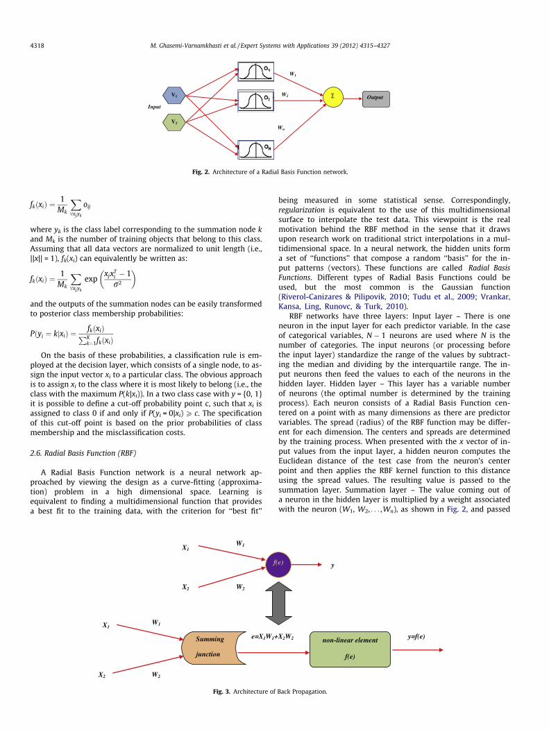
Fig. 2. Architecture of a Radial Basis Function network.


fkðxiÞ ¼1

Mk

X8xjyk

oij

where yk is the class label corresponding to the summation node kand Mk is the number of training objects that belong to this class.Assuming that all data vectors are normalized to unit length (i.e.,||x|| = 1), fk(xi) can equivalently be written as:

fkðxiÞ ¼1

Mk

X8xjyk

expxjxT

i � 1r2

� �

and the outputs of the summation nodes can be easily transformedto posterior class membership probabilities:

Pðyi ¼ kjxiÞ ¼fkðxiÞPKk¼1fkðxiÞ

On the basis of these probabilities, a classification rule is em-ployed at the decision layer, which consists of a single node, to as-sign the input vector xi to a particular class. The obvious approachis to assign xi to the class where it is most likely to belong (i.e., theclass with the maximum P(k|xi)). In a two class case with y = {0, 1}it is possible to define a cut-off probability point c, such that xi isassigned to class 0 if and only if P(yi = 0|xi) P c. The specificationof this cut-off point is based on the prior probabilities of classmembership and the misclassification costs.

2.6. Radial Basis Function (RBF)

A Radial Basis Function network is a neural network ap-proached by viewing the design as a curve-fitting (approxima-tion) problem in a high dimensional space. Learning isequivalent to finding a multidimensional function that providesa best fit to the training data, with the criterion for ‘‘best fit’’

f(

W1

W2

X1

X2

Summing

junction

W2

W1X1

X2

e=X1W1+

Fig. 3. Architecture of

being measured in some statistical sense. Correspondingly,regularization is equivalent to the use of this multidimensionalsurface to interpolate the test data. This viewpoint is the realmotivation behind the RBF method in the sense that it drawsupon research work on traditional strict interpolations in a mul-tidimensional space. In a neural network, the hidden units forma set of ‘‘functions’’ that compose a random ‘‘basis’’ for the in-put patterns (vectors). These functions are called Radial BasisFunctions. Different types of Radial Basis Functions could beused, but the most common is the Gaussian function(Riverol-Canizares & Pilipovik, 2010; Tudu et al., 2009; Vrankar,Kansa, Ling, Runovc, & Turk, 2010).

RBF networks have three layers: Input layer – There is oneneuron in the input layer for each predictor variable. In the caseof categorical variables, N � 1 neurons are used where N is thenumber of categories. The input neurons (or processing beforethe input layer) standardize the range of the values by subtract-ing the median and dividing by the interquartile range. The in-put neurons then feed the values to each of the neurons in thehidden layer. Hidden layer – This layer has a variable numberof neurons (the optimal number is determined by the trainingprocess). Each neuron consists of a Radial Basis Function cen-tered on a point with as many dimensions as there are predictorvariables. The spread (radius) of the RBF function may be differ-ent for each dimension. The centers and spreads are determinedby the training process. When presented with the x vector of in-put values from the input layer, a hidden neuron computes theEuclidean distance of the test case from the neuron’s centerpoint and then applies the RBF kernel function to this distanceusing the spread values. The resulting value is passed to thesummation layer. Summation layer – The value coming out ofa neuron in the hidden layer is multiplied by a weight associatedwith the neuron (W1, W2, . . . ,Wn), as shown in Fig. 2, and passed

e) y

non-linear element

f(e)

y=f(e) X2W2

Back Propagation.

Table 1Statistics on aftertaste attributes of non-alcoholic beer.

Attribute Non-alcoholic beer brand Mean Standard deviation*

P1 P2 P3 P4 P5 P6 P7

Bitter 2 (0.272)** 2.04 (0.23) 1.33 (0.384) 1.43 (0.417) 4.05 (0.448) 1.95 (0.23) 1.19 (0.262) 2 0.968Sour 0.19 (0.262) 0.09 (0.162) 0.67 (0.272) 0.09 (0.162) 0 (0) 0.23 (0.37) 0.33 (0.33) 0.23 0.22Sweet 0.95 (0.23) 0.19 (0.262) 0.23 (0.418) 1.9 (0.37) 1.14 (0.179) 0.14 (0.179) 0.24 (0.371) 0.69 0.671Fruity 0.95 (0.3) 0.28 (0.355) 0.86 (0.178) 0 (0) 0.95 (0.126) 0.09 (0.162) 2.09(0.252) 0.75 0.72Liquorice 0.62 (0.23) 0.09 (0.163) 0.14 (0.262) 0.09 (0.163) 0.05 (0.126) 0.19 (0.262) 0.14 (0.178) 0.19 0.194Body 4.76 (0.252) 1.43 (0.317) 4.05 (0.3) 4.14 (0.325) 5.24 (0.371) 2.28 (0.23) 4.09 (0.499) 3.71 1.362Artificial 0 (0) 0 (0) 0 (0) 0 (0) 0 (0) 0.28 (0.3) 0.24 (0.252) 0.07 0.128Duration 5.81 (0.262) 5.19 (0.378) 4.05 (0.126) 2 (0.192) 3.90 (0.163) 1.95 (0.126) 1.71 (0.356) 3.52 1.658Intensity 5.86 (0.325) 5.05 (0.23) 4.05 (0.405) 1.86 (0.262) 3.95 (0.356) 2 (0.192) 2.05 (0.405) 3.54 1.607

* Standard deviation was the square root of the error variance of ANOVA.** The numbers in parenthesis are standard deviation.

Table 2Variance analysis of the interaction effects of assessor, non-alcoholic beer brands onbitterness sensory evaluation.

Source of variations Degree offreedom

Sum ofsquare

Meansquare

F

Assessor 6 6.09 1.01 3.11b

Beer brand 6 118.09 19.68 60.27a

Assessor � beer brand 36 7.80 0.21 0.66b

Error 98 32 0.33 –

a Corresponding to confident of interval 95%.b Corresponding to no marked difference.

Table 3Classification of non-alcoholic beer brands based on Duncan’s multiple range test.

Attributes Categories (class)*

A B C D E F

Bitter P5 P1, P2, P6 P3, P4 P7Sour P3 P7 P6 P1 P2, P4 P5Sweet P4 P5 P1 P3, P7 P2 P6Fruity P7 P1, P3, P5 P2 P6 P4Liquorice P1 P6 P3, P7 P2, P4 P5Body P1, P5 P3, P4, P7 P2, P6Artificial P6 P7 P1, P2, P3, P4, P5Duration P1 P2 P3, P5 P4, P6 P7Intensity P1 P2 P3, P5 P4, P6, P7

* The classes are in descending order, i.e. Classes A and F have the greatest and thelowest values of an attribute, respectively.


to the summation which adds up the weighted values and pre-sents this sum as the output of the network. Not shown in thisfigure, it is a bias value of 1.0 that is multiplied by a weight W0

and fed into the summation layer. For classification problems,there is one output (and a separate set of weights and summa-tion unit) for each target category. The value output for a cate-gory is the probability that the case being evaluated has thatcategory. These parameters are determined by the training pro-cess: The number of neurons in the hidden layer, the coordinatesof the center of each hidden-layer RBF function, the radius(spread) of each RBF function in each dimension and the weightsapplied to the RBF function outputs as they are passed to thesummation layer (Pretty, Vega, Ochando, & Tabares, 2010).

2.7. Back Propagation (BP)

Since the real uniqueness or ‘intelligence’ of the network existsin the values of the weights between neurons, we need a method ofadjusting the weights to solve a particular problem. For this type ofnetwork, the most common learning algorithm is called Back Prop-agation (BP). As shown in Fig 3, the multiplayer perceptron (MLP)model using the Back Propagation (BP) algorithm is one of thewell-known neural network classifiers which consist of sets ofnodes arranged in multiple layers with connections only betweennodes in the adjacent layers by weights. The layer where the inputsinformation is presented is known as the input layer. The layerwhere the processed information is retrieved is called the outputlayer. All layers between the input and output layers are knownhidden layers. For all nodes in the network, except the input layernodes, the total input of each node is the sum of weighted outputsof the nodes in the previous layer. Each node is activated with theinput to the node and the activation function of the node (Chen,Chen, & Kuo, 2010).

The input and output of the node i (except for the input layer) ina MLP mode, according to the BP algorithm, is:

Input : Xi ¼X

WijOi þ bi ð1ÞOutput : Oi ¼ f ðXiÞ ð2Þ

where Wij: the weight of the connection from node i to node j, Bi:the numerical value called bias, F: the activation function.

The sum in Eq. (1) is over all nodes j in the previous layer. The out-put function is a non-linear function which allows a network to solveproblems that a linear network cannot solve. In this study the Sig-moid function given in Eq. (3) is used to determine the output state.

FðXiÞ ¼ 1=ð1þ expð�XiÞ ð3Þ

Back Propagation (BP) learning algorithm is designed to reducean error between the actual output and the desired output of the

network in a gradient descent manner. The summed squared error(SSE) is defined as:

SSE ¼ 1=2X

pi

XOpi � Tpi

!2

ð4Þ

where p index the all training patterns and i indexes the outputnodes of the network. Opi and Tpi denote the actual output and thedesired output of node, respectively when the input vector p is ap-plied to the network.

A set of representative input and output patterns is selected totrain the network. The connection weight Wij is adjusted wheneach input pattern is presented. All the patterns are repeatedly pre-sented to the network until the SSE function is minimized and thenetwork ‘‘learns’’ the input patterns (Zhu et al., 2010). An applica-tion of the gradient descent method yields the following iterativeweight update rule:

DWijðnþ 1Þ ¼ gðdiOi þ aDWijðnÞ ð5Þ

where D: the learning factor, a: the momentum factor, di: the nodeerror, for output node i is then given as


di ¼ ðti � OiÞOið1� OiÞ ð6Þ

The node error at an arbitrary hidden node is

di ¼ Oið1� OjÞX

k

dkWki

(a) (

(e) (

(g)

(c)

Fig. 4. Polar plots of the panelists response to aftertaste attributes of seven non-alcoholibrand P6, (g) brand P7.

Each neuron is composed of two units. First unit adds productsof weights coefficients and input signals. The second unit realizesnon-linear function, called neuron activation function. Signal e isadder output signal, and y = f(e) is output signal of non-linear ele-ment. Signal y is also output signal of neuron.

b)

f)

(d)

c beer brands: (a) brand P1, (b) brand P2, (c) brand P3, (d) brand P4, (e) brand P5, (f)


3. Results and discussions

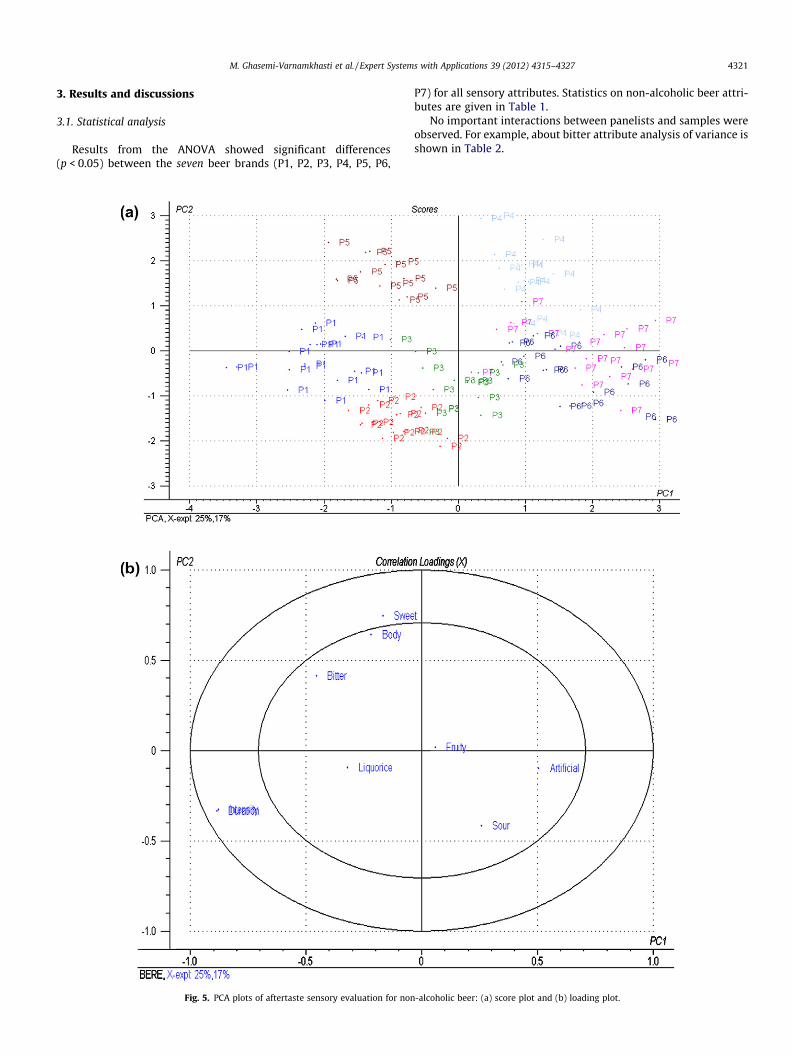
3.1. Statistical analysis

Results from the ANOVA showed significant differences(p < 0.05) between the seven beer brands (P1, P2, P3, P4, P5, P6,

Fig. 5. PCA plots of aftertaste sensory evaluation for non

P7) for all sensory attributes. Statistics on non-alcoholic beer attri-butes are given in Table 1.

No important interactions between panelists and samples wereobserved. For example, about bitter attribute analysis of variance isshown in Table 2.

-alcoholic beer: (a) score plot and (b) loading plot.


Therefore, Duncan’s multiple ranges test was performed formeans comparison among the beer brands. This statistical testwas used for all nine attributes to develop the categories. The cat-egories are given in Table 3. It is clear from this table that the prod-ucts with similar letter have not significant difference for a specificaftertaste attribute.

An awareness of these categories could be of interest to brew-ers; for example about bitter, the information obtained on bitter-ness value could give an insight into process control to brewer,since the causes of bitter taste is: content and alpha strength;length of hop boil; presence of dark malts, alkaline water and itcan be reduced by lower alpha hops, hops added at stages through

Fig. 6. PLS-DA score plot corresponding to t

boil, filtration, high temperature ferment. So, a brewer can checkthe beer production line that whether bitterness value of the beerprocessed is within the categories considered or not. Then, beerproduction manager decide about these items: How long hops areboiled, type of hop, fermentation temperature (high temperatureand quick fermentation decrease bitterness), filtration reducesbitterness.

The polar plots of the average scores of the panelists for nineaftertaste attributes in seven non-alcoholic beer brands are shownin Fig. 4, in terms of relative response changes. The contour of thesepolar plots differs from one sample to another, illustrating the dis-crimination capabilities of the panel. These contour could be com-

he classification of non-alcoholic beers.

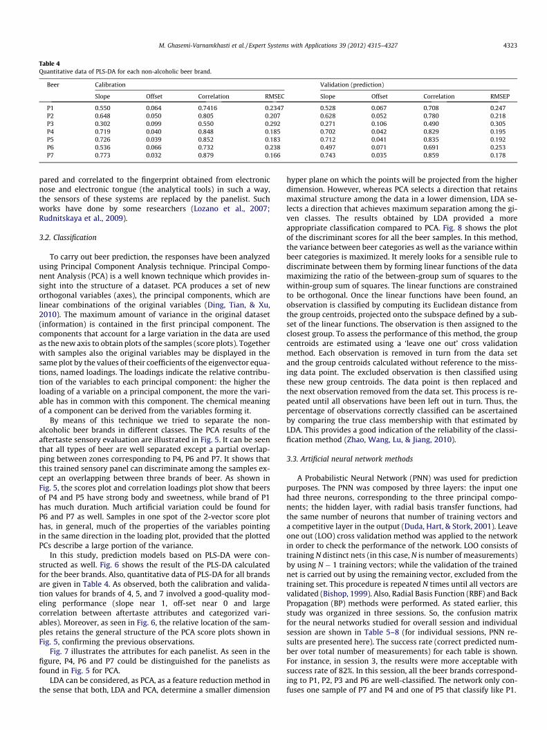
Table 4Quantitative data of PLS-DA for each non-alcoholic beer brand.

Beer Calibration Validation (prediction)

Slope Offset Correlation RMSEC Slope Offset Correlation RMSEP

P1 0.550 0.064 0.7416 0.2347 0.528 0.067 0.708 0.247P2 0.648 0.050 0.805 0.207 0.628 0.052 0.780 0.218P3 0.302 0.099 0.550 0.292 0.271 0.106 0.490 0.305P4 0.719 0.040 0.848 0.185 0.702 0.042 0.829 0.195P5 0.726 0.039 0.852 0.183 0.712 0.041 0.835 0.192P6 0.536 0.066 0.732 0.238 0.497 0.071 0.691 0.253P7 0.773 0.032 0.879 0.166 0.743 0.035 0.859 0.178


pared and correlated to the fingerprint obtained from electronicnose and electronic tongue (the analytical tools) in such a way,the sensors of these systems are replaced by the panelist. Suchworks have done by some researchers (Lozano et al., 2007;Rudnitskaya et al., 2009).

3.2. Classification

To carry out beer prediction, the responses have been analyzedusing Principal Component Analysis technique. Principal Compo-nent Analysis (PCA) is a well known technique which provides in-sight into the structure of a dataset. PCA produces a set of neworthogonal variables (axes), the principal components, which arelinear combinations of the original variables (Ding, Tian, & Xu,2010). The maximum amount of variance in the original dataset(information) is contained in the first principal component. Thecomponents that account for a large variation in the data are usedas the new axis to obtain plots of the samples (score plots). Togetherwith samples also the original variables may be displayed in thesame plot by the values of their coefficients of the eigenvector equa-tions, named loadings. The loadings indicate the relative contribu-tion of the variables to each principal component: the higher theloading of a variable on a principal component, the more the vari-able has in common with this component. The chemical meaningof a component can be derived from the variables forming it.

By means of this technique we tried to separate the non-alcoholic beer brands in different classes. The PCA results of theaftertaste sensory evaluation are illustrated in Fig. 5. It can be seenthat all types of beer are well separated except a partial overlap-ping between zones corresponding to P4, P6 and P7. It shows thatthis trained sensory panel can discriminate among the samples ex-cept an overlapping between three brands of beer. As shown inFig. 5, the scores plot and correlation loadings plot show that beersof P4 and P5 have strong body and sweetness, while brand of P1has much duration. Much artificial variation could be found forP6 and P7 as well. Samples in one spot of the 2-vector score plothas, in general, much of the properties of the variables pointingin the same direction in the loading plot, provided that the plottedPCs describe a large portion of the variance.

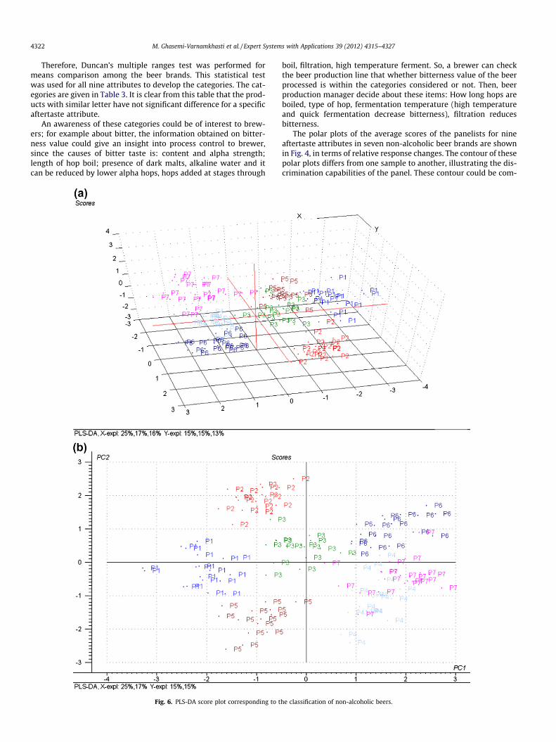
In this study, prediction models based on PLS-DA were con-structed as well. Fig. 6 shows the result of the PLS-DA calculatedfor the beer brands. Also, quantitative data of PLS-DA for all brandsare given in Table 4. As observed, both the calibration and valida-tion values for brands of 4, 5, and 7 involved a good-quality mod-eling performance (slope near 1, off-set near 0 and largecorrelation between aftertaste attributes and categorized vari-ables). Moreover, as seen in Fig. 6, the relative location of the sam-ples retains the general structure of the PCA score plots shown inFig. 5, confirming the previous observations.

Fig. 7 illustrates the attributes for each panelist. As seen in thefigure, P4, P6 and P7 could be distinguished for the panelists asfound in Fig. 5 for PCA.

LDA can be considered, as PCA, as a feature reduction method inthe sense that both, LDA and PCA, determine a smaller dimension

hyper plane on which the points will be projected from the higherdimension. However, whereas PCA selects a direction that retainsmaximal structure among the data in a lower dimension, LDA se-lects a direction that achieves maximum separation among the gi-ven classes. The results obtained by LDA provided a moreappropriate classification compared to PCA. Fig. 8 shows the plotof the discriminant scores for all the beer samples. In this method,the variance between beer categories as well as the variance withinbeer categories is maximized. It merely looks for a sensible rule todiscriminate between them by forming linear functions of the datamaximizing the ratio of the between-group sum of squares to thewithin-group sum of squares. The linear functions are constrainedto be orthogonal. Once the linear functions have been found, anobservation is classified by computing its Euclidean distance fromthe group centroids, projected onto the subspace defined by a sub-set of the linear functions. The observation is then assigned to theclosest group. To assess the performance of this method, the groupcentroids are estimated using a ‘leave one out’ cross validationmethod. Each observation is removed in turn from the data setand the group centroids calculated without reference to the miss-ing data point. The excluded observation is then classified usingthese new group centroids. The data point is then replaced andthe next observation removed from the data set. This process is re-peated until all observations have been left out in turn. Thus, thepercentage of observations correctly classified can be ascertainedby comparing the true class membership with that estimated byLDA. This provides a good indication of the reliability of the classi-fication method (Zhao, Wang, Lu, & Jiang, 2010).

3.3. Artificial neural network methods

A Probabilistic Neural Network (PNN) was used for predictionpurposes. The PNN was composed by three layers: the input onehad three neurons, corresponding to the three principal compo-nents; the hidden layer, with radial basis transfer functions, hadthe same number of neurons that number of training vectors anda competitive layer in the output (Duda, Hart, & Stork, 2001). Leaveone out (LOO) cross validation method was applied to the networkin order to check the performance of the network. LOO consists oftraining N distinct nets (in this case, N is number of measurements)by using N � 1 training vectors; while the validation of the trainednet is carried out by using the remaining vector, excluded from thetraining set. This procedure is repeated N times until all vectors arevalidated (Bishop, 1999). Also, Radial Basis Function (RBF) and BackPropagation (BP) methods were performed. As stated earlier, thisstudy was organized in three sessions. So, the confusion matrixfor the neural networks studied for overall session and individualsession are shown in Table 5–8 (for individual sessions, PNN re-sults are presented here). The success rate (correct predicted num-ber over total number of measurements) for each table is shown.For instance, in session 3, the results were more acceptable withsuccess rate of 82%. In this session, all the beer brands correspond-ing to P1, P2, P3 and P6 are well-classified. The network only con-fuses one sample of P7 and P4 and one of P5 that classify like P1.

Panelist A

0

1

2

3

4

5

6

1

2

3

45

6

7BitterSweetSourFruityLiquoriceBodyAtrificialDurationIntensity

Panelist B

0

1

2

3

4

5

6

1

2

3

45

6

7

BitterSweetSourFruityLiquoriceBodyAtrificialDurationIntensity

Panelist C

0

1

2

3

4

5

6

7

1

2

3

45

6


Panelist D

0

1

2

3

4

5

6

1

2

3

45

6


Panelist E

0

1

2

3

4

5

6

1

2

3

45

6

7


Panelist F

0

1

2

3

4

5

6

7

1

2

3

45

6

7


Panelist G

0

1

2

3

4

5

6

1

2

3

45

6


Fig. 7. Polar plots of the panelists’ response to aftertaste attributes of seven non-alcoholic (the numbers around the plots are the beer brands).


The highest success rate to classify the beer brands was ob-tained in RBF approach as 0.9727 as seen in Table 9.

The BP network topology was formed by three layers: the inputlayer has two neurons corresponding to the first two components,a variable number in hidden layer, and seven neurons in the outputlayer corresponding to the seven beer brands. The network

processes the inputs and compares its outputs against the desiredoutputs. Errors are then propagated back through the system,causing the system to adjust the weights that control the network.This process occurs over and over as the weights are continuallytweaked. During the training of a network the same set of data isprocessed many times as the connection weights are always

-0.8 -0.6 -0.4 -0.2 0 0.2 0.4 0.6 0.8-0.8

-0.6

-0.4

-0.2

0

0.2

0.4

0.6

DF1

DF2

P1

P2

P3

P4

P5

P6

P7

Fig. 8. Score plots of seven different non-alcoholic beer brands by LDA.

Table 5Confusion matrix for the PNN prediction for whole sessions.

Real/predicted P1 P2 P3 P4 P5 P6 P7

P1 18 1 1 0 1 0 0P2 0 21 0 0 0 0 0P3 0 0 20 0 0 0 1P4 0 0 0 9 0 2 10P5 1 0 0 0 20 0 0P6 0 0 0 2 0 19 0P7 0 0 0 8 0 1 12

Success rate 0.80952381

Table 6Confusion matrix for the PNN prediction for session 1.


P1 5 1 1 0 0 0 0P2 1 6 0 0 0 0 0P3 1 0 5 1 0 0 0P4 0 0 0 3 0 1 3P5 0 0 0 0 7 0 0P6 0 0 0 1 0 6 0P7 0 0 0 3 0 1 3




P1 7 0 0 0 0 0 0P2 0 7 0 0 0 0 0P3 0 0 7 0 0 0 0P4 0 0 0 2 0 1 4P5 0 0 0 0 7 0 0P6 0 0 0 0 0 5 2P7 0 0 0 4 0 1 2




P1 7 0 0 0 0 0 0P2 0 7 0 0 0 0 0P3 0 0 7 0 0 0 0P4 0 0 0 3 0 1 3P5 1 0 0 0 6 0 0P6 0 0 0 0 0 7 0P7 0 0 0 4 0 0 3


Table 9Confusion matrix for the RBF prediction for whole sessions.


P1 21 0 0 0 0 0 0P2 0 21 0 0 0 0 0P3 1 0 20 0 0 0 0P4 0 0 0 19 0 1 1P5 0 0 0 0 21 0 0P6 0 0 0 0 0 21 0P7 0 0 1 0 0 0 20


Fig. 9. Success rate values in different neurons number in hidden layer in BackPropagation method.

Table 10Confusion matrix with 14 neurons in hidden layer for the RBF prediction for wholesessions.

Classification P1 P2 P3 P4 P5 P6 P7

P1 20 0 0 0 1 0 0P2 1 20 0 0 0 0 0P3 1 0 20 0 0 0 0P4 0 1 0 20 0 0 0P5 1 0 0 1 19 0 0P6 1 0 0 0 0 20 0P7 0 0 0 0 1 0 20



refined. The samples were divided into two groups training set andthe testing set. In the training of the network, different number ofneurons in the hidden layer has been tested in two proofs. Theresult is shown in Fig 9. The optimal number turned out to be 14neurons by several times tested. The classification success is


100% for the training set in total and 97% for the testing set in total.The result of the testing set is shown in Table 10.

All together, among the methods used, Radial Basis Functions(RBF) showed the greatest accuracy in beer classification. This ap-proach has attracted a great deal of interest due to their rapidtraining, generality and simplicity. When compared with tradi-tional multilayer perceptrons, RBF networks present a much fastertraining, without having to cope with traditional Back Propagationproblems, such as network paralysis and the local minima. Theseimprovements have been achieved without compromising the gen-erality of applications.

The results obtained in the current study could be correlatedwith biomimetic-based devices such as electronic nose and tonguesystems (Ghasemi-Varnamkhasti, Mohtasebi, Rodriguez-Mendez,Lozano, et al., 2011; Ghasemi-Varnamkhasti, Mohtasebi,Rodriguez-Mendez, Siadat, et al., 2011; Ghasemi-Varnamkhasti,Mohtasebi, & Siadat, 2010; Wei, Hu, et al., 2009; Wei, Wang, & Liao,2009). Since sensory evaluation tests are time consuming andrequire complex and expensive equipment. Then, e-tongue ande-nose as innovative analytical tools could be used instead of sen-sory evaluation. It is hoped that the correlation of these resultswith e-tongue and e-nose to be promising. According to thebibliography, such works have shown a very good correlation withhuman gustatory sensation (Kovacs, Sipos, Kantor, Kokai, & Fekete,2009; Lozano et al., 2007; Uchida et al., 2001). A similar approach isthe adsorption and desorption of beer and coffee on a lipid mem-brane simulating the bitter reception of the tongue. The measure-ment of bitter intensities and durations showed good correlation tosensory experiments (Kaneda & Takashio, 2005; Kaneda, Watari,Takshio, & Okahata, 2003).

At the end of this paper, this is worth mentioning that bitter-ness is the most important organoleptic characteristic of non-alcoholic beer and not only the intensity but also the durationaffects the bitter quality of beer in a sensory evaluation. Bitternessis one of the flavor items in the matching test and a criterion for thedescriptive ability, used for selection and training of assessors. Asemphasized in the literature (Kaneda, Shinotsuka, Kobayakawa,Saito, & Okakata, 2000), the time-intensity rating of bitterness pro-vides a category scaling and additional information, including ratesof increase and decrease of bitterness, persistence of maximumintensity, changes caused by swallowing, and duration of after-taste.

The above issues are recommended to be studied in future.Since practical problems associated with the sensory assessmentof non-alcoholic beer and other foodstuffs are well known, trainingand maintaining of the professional sensory panels is necessary forensuring reproducibility of the results but expensive. Anotherproblem is a rapid saturation of the assessors meaning that onlya limited number of samples may be assessed during the sametasting session (Rudnitskaya et al., 2009). As a consequent, sensoryanalysis is notorious for being slow, expensive and sometimes suf-fering from irreproducibility even when professional panels are in-volved. It is stated that significant efforts are being directed to thedevelopment of instrumental methods for routine analysis of tasteattributes of foodstuffs and beer in particular (Rudnitskaya et al.,2009). However, sensory analysis suffers from an objective, unbi-ased, and reproducible evaluation, this necessitate the statisticalhandling of the data. Recently, taste and odor evaluations usingmembrane sensors, which are supposed to reflect olfactory andgustatory characteristics of the human nose and tongue, have beenactively studied (Ghasemi-Varnamkhasti, 2011; Ghasemi-Varnamkhasti et al., 2010; Hayashi, Chen, Ikezaki, & Ujihara,2008; Peres, Dias, Barcelos, Sa Morais, & Marchado, 2009;Rodriguez-Mendez et al., 2004; Rudnitskaya et al., 2006; Wei, Hu,et al., 2009; Wei, Wang, et al., 2009). An electronic aroma detectorhas been introduced for quality control in the brewing industry,

e.g., for differentiation between beers and for recognition of thepresence of important beer aromas and variety/quality parameters.The results obtained from the current study could be considered asa reference data in such systems (e-tongue and e-nose). There aremany reports on the correlation of the output of electronic nosesand tongues to sensory data, and in many the sensory part of thedata is implied rather than measured. However, the prospects forthese kinds of devices are very good, and we expect to see manyvariants of machine smell/taste/sight systems in the future.

4. Conclusions

The sensory evaluation of non-alcoholic beer plays a relevantrole for the quality and properties of the commercialized product.In this contribution, we did a sensory evaluation of aftertaste attri-butes for non-alcoholic beer. We used seven beer brands to evalu-ate nine attributes by a trained sensory panel. The results showedthat the data are in consistent. Therefore, the brands were statisti-cally classified in some categories. Effect of panelist was found tobe statistically insignificant. Also, neural network methods showeda promising result for prediction of beer brands in such a way thesuccess rate (correct predicted number over total number of mea-surements) was found to be acceptable. Among the methods used,Radial Basis Functions (RBF) showed the greatest accuracy in beerclassification.

It is important that a proper grounding in basic experimentaldesign and statistics is given when training sensory scientists. Thiswill encourage a wider understanding of possible manipulations ofdata, and ultimately result in better products. This study could begone on another research in which electronic nose and tonguewould be used to evaluate non-alcoholic beer quality (Ghasemi-Varnamkhasti, 2011). As found in this study, the results are suit-able as a reliable reference data to be considered in multi arraysof sensors and the results on aftertaste sensory evaluation couldbe correlated to the data obtained from electronic nose and tonguein a separate research.

Acknowledgments

The support of the Iran National Science Foundation (INSF) isgratefully appreciated regarding the finance of this research.

References

Arrieta, A. A., Rodriguez-Mendez, M. L., de Saja, J. A., Blanco, C. A., & Nimubona, D.(2010). Prediction of bitterness and alcoholic strength in beer using anelectronic tongue. Food Chemistry, 123, 642–646.

Bamforth, C. W. (2000). Brewing and brewing research: Past, present and future.Journal of the Science of Food and Agriculture, 80, 1371–1378.

Barker, M., & Rayens, W. (2003). Partial least squares for discrimination. Journal ofChemometrics, 17(3), 166–173.

Bishop, C. M. (1999). Neural networks for pattern recognition. Oxford: OxfordUniversity Press.

Chen, F., Chen, Y., & Kuo, J. (2010). Applying moving back-propagation neuralnetwork and moving fuzzy neuron network to predict the requirement ofcritical spare parts. Expert Systems with Applications, 37, 4358–4367.

Daems, V., & Delvaux, F. (1997). Multivariate analysis of descriptive sensory data on40 commercial beers. Food Quality and Preference, 8, 373–380.

Ding, M., Tian, Z., & Xu, H. (2010). Adaptive kernel principal component analysis.Signal Processing, 90, 1542–1553.

Duda, R. O., Hart, P. E., & Stork, D. G. (2001). Pattern classification (pp. 115–117).Wiley-Interscience.

Dutta, K., Prakash, N., & Kaushik, S. (2010). Probabilistic neural network approach tothe classification of demonstrative pronouns for indirect anaphora in Hindi.Expert Systems with Applications, 37, 5607–5613.

Ghasemi-Varnamkhasti, M., Mohtasebi, S. S., & Siadat, M. (2010). Biomimetic-basedodor and taste sensing systems to food quality and safety characterization: Anoverview on basic principles and recent achievements. Journal of FoodEngineering, 100, 377–387.

Ghasemi-Varnamkhasti, M. (2011). Design, development and implementation of ametal oxide semiconductor (MOS) based machine olfaction system andbioelectronic tongue to quality change detection of beers coupled with


pattern recognition analysis techniques. PhD Thesis, University of Tehran, Karaj,Iran.

Ghasemi-Varnamkhasti, M., Mohtasebi, S. S., Siadat, M., Ahmadi, H., Razavi, S. H., &Dicko, A. (2011). Aging fingerptint characterization of beer using electronicnose. Sensors and Actuators B, 159, 51–59.

Ghasemi-Varnamkhasti, M., Mohtasebi, S. S., Rodriguez-Mendez, M. L., Siadat, M.,Ahmadi, H., & Razavi, S. H. (2011). Electronic and bioelectronic tongues, twopromising analytical tools for the quality evaluation of non alcoholic beer.Trends in Food Science and Technology, 22, 245–248.

Ghasemi-Varnamkhasti, M., Mohtasebi, S. S., Rodriguez-Mendez, M. L., Lozano, J.,Razavi, S. H., & Ahmadi, H. (2011). Potential application of electronic nosetechnology in brewery. Trends in Food Science and Technology, 22, 165–174.

Haseleu, G., Intelmann, D., & Hofmann, T. (2009). Structure determination andsensory evaluation of novel bitter compounds formed from b-acids of hop(Humulus lupulus L.) upon wort boiling. Food Chemistry, 116, 71–81.

Hayashi, N., Chen, R., Ikezaki, H., & Ujihara, T. (2008). Evaluation of the umami tasteintensity of green tea by taste sensor. Journal of Agricultural and Food Chemistry,56, 7384–7387.

Hsieh, S., & Chen, C. (2009). Adaptive image interpolation using probabilistic neuralnetwork. Expert Systems with Applications, 36, 6025–6029.

Kaneda, H., Shinotsuka, K., Kobayakawa, T., Saito, S., & Okakata, Y. (2000). Evaluationof beer bitterness by measuring the adsorption on a lipid-coated quartz-crystalmicrobalance. Journal of the Institute of Brewing, 106(5), 305–309.

Kaneda, H., & Takashio, M. (2005). Development of beer taste sensor using a lipid-coated quartz-crystal microbalance. Journal of American Society of BrewingChemist, 63(3), 89–95.

Kaneda, H., Watari, J., Takshio, M., & Okahata, Y. (2003). Adsorption and desorptionof beer and coffee on an lipid membrane as related to sensory bitterness. Journalof the Institute of Brewing, 109, 127–133.

Kovacs, Z., Sipos, L., Kantor, D. B., Kokai, Z., & Fekete, A. (2009). Mineral water tasteattributes evaluated by sensory panel and electronic tongue. In Olfaction andelectronic nosed, proceedings of the 13th international symposium 15–17 April,2009, Brescia, Italy.

Langstaff, S. A., Guinard, J. X., & Lewis, M. J. (1991). Sensory evaluation of themouthfeel of beer. American Society of Brewing Chemists Journal, 49(2), 54–59.

Lozano, J., Santos, J. P., Arroyo, T., Aznar, M., Cabellos, J. M., Gil, M., et al. (2007).Correlating e-nose response to wine sensorial descriptors and gaschromatography-mass spectrometry profiles using partial least squareregression analysis. Sensors and Actuators B: Chemical, 127, 267–276.

Mejlholm, O., & Martens, M. (2006). Beer identity in Denmark. Food Quality andPreference, 17, 108–115.

Peres, A. M., Dias, L. G., Barcelos, T. P., Sa Morais, J., & Marchado, A. A. S. C. (2009). Anelectronic tongue for juice level evaluation in non-alcoholic beverage. ProcediaChemistry, 1, 1023–1026.

Porretta, S., & Donadini, G. (2008). A preference study for no alcoholic beer in Italyusing quantitative concept analysis. Journal of the Institute of Brewing, 114(4),315–321.

Pretty, D. G., Vega, J., Ochando, M. A., & Tabares, F. L. (2010). Empirically derivedbasis functions for unsupervised classification of radial profile data. FusionEngineering and Design, 85, 423–424.

Riverol-Canizares, C., & Pilipovik, V. (2010). The use of radial basis functionnetworks (RBFN) to predict critical water parameters in desalination plants.Expert Systems with Applications, 37, 7285–7287.

Rodriguez-Mendez, M. L., Arrieta, A. A., Parra, V., Bernal, A., Vegas, A., Villanueva, S.,et al. (2004). Fusion of three sensory modalities for the multimodalcharacterization of red wines. IEEE Sensors Journal, 4(3), 348–354.

Rudnitskaya, A., Kirsanov, D., Legin, A., Beullens, K., Lammertyn, J., Nicolai, B. M.,et al. (2006). Analysis of apples varieties-comparison of electronic tongue withdifferent analytical techniques. Sensors and Actuators B: Chemical, 116, 23–28.

Rudnitskaya, A., Polshin, E., Kirsanov, D., Lammertyn, J., Nicolai, B., Saison, D., et al.(2009). Instrumental measurement of beer taste attributes using an electronictongue. Analytica Chemica Acta, 646, 111–118.

Specht, D. F. (1990). Probabilistic neural networks. Neural Networks, 3(1), 109–118.Tudu, B., Jana, A., Metla, A., Ghosh, D., Bhattacharyya, N., & Bandyopadhyay, R.

(2009). Electronic nose for black tea quality evaluation by an incremental RBFnetwork. Sensors and Actuators B: Chemical, 138, 90–95.

Uchida, T., Kobayashi, Y., Miyanaga, Y., Toukubo, R., Ikezaki, H., Taniguchi, A., et al.(2001). A new method for evaluating the bitterness of medicines by semi-continuous measurement of adsorption using a taste sensor. Chemical andPharmaceutical Bulletin, 49(10), 1336–1339.

Vrankar, L., Kansa, E. J., Ling, L., Runovc, F., & Turk, G. (2010). Moving-boundaryproblems solved by adaptive radial basis functions. Computers and Fluids, 39,1480–1490.

Wei, H., Hu, X., Zhao, L., Liao, X., Zhang, Y., Zhang, M., et al. (2009). Evaluation ofChinese tea by the electronic tongue: Correlation with sensory properties andclassification according to geographical origin and grade level. Food ResearchInternational, 42, 1462–1467.

Wei, Z., Wang, J., & Liao, W. (2009). Technique potential for classification of honeyby electronic tongue. Journal of Food Engineering, 94(3–4), 260–266.

Yin, Y., & Ding, Y. (2009). A close to real-time prediction method of total coliformbacteria in foods based on image identification technology and artificial neuralnetwork. Food Research International, 42, 191–199.

Zhao, Y., Wang, J., Lu, Q., & Jiang, R. (2010). Pattern recognition of eggshell crackusing PCA and LDA. Innovative Food Science and Emerging Technologies, 11,520–525.

Zhu, X., Li, S., Shan, Y., Zhang, Z., Li, G., Su, D., et al. (2010). Detection of adulterantssuch as sweeteners materials in honey using near-infrared spectroscopy andchemometrics. Journal of Food Engineering, 101, 92–97.

classification of non-alcoholic beer based on aftertaste sensory

Documents