RESEARCH REPORT October 2002 RR-02-20

Classical Test Theory as a First-Order Item Response Theory: Application to True-Score Prediction From a Possibly Nonparallel Test

Paul W. Holland Machteld Hoskens

Research & Development Division Princeton, NJ 08541

Classical Test Theory as a First-Order Item Response Theory:

Application to True-Score Prediction From a Possibly Nonparallel Test

Paul W. Holland, Educational Testing Service

Machteld Hoskens, CTB-McGraw Hill

October 2002

Research Reports provide preliminary and limited dissemination of ETS research prior to publication. They are available without charge from:

Research Publications Office Mail Stop 10-R Educational Testing Service Princeton, NJ 08541

i

Abstract

We give an account of classical test theory (CTT) in terms of the more fundamental ideas of item

response theory (IRT). This approach views CTT as a very general version of IRT, and the

commonly used IRT models as detailed elaborations of CTT for special purposes. We then use

this approach to CTT to derive some general results regarding the prediction of the true score of

a test from an observed score on that test as well from an observed score on a different test. This

leads us to a new view of linking tests that were not developed to be linked to each other. In

addition we propose true-score prediction analogues of the Dorans and Holland measures of the

population sensitivity of test linking functions. We illustrate the accuracy of the first-order theory

using simulated data from the Rasch model and illustrate the effect of population differences

using a set of real data.

Key words: test theory, true scores, best linear predictors, test linking, nonparallel tests,

simulation, Rasch Model

ii

Acknowledgements

We would like to thank Neil Dorans, Skip Livingston, and two anonymous referees for many

suggestions that have greatly improved this paper. The work reported here is collaborative in

every respect and the order of authorship is alphabetical. It was begun while both authors were

on the faculty at the Graduate School of Education, University of California, Berkeley.

1

1. Introduction

This paper has two tasks. The first is to show how classical test theory (CTT) can be

viewed as a mean and variance (i.e., first-order) approximation to a very general version of item

response theory (IRT). This task connects CTT more closely to IRT and provides simplified

ways of making calculations relevant to IRT models using the easier mean and variance

calculations of CTT. It is often hard to see the structure of a full IRT model through the forest of

item response functions, their numerous parameters, prior ability distributions, complex

estimation techniques, the computation of plausible values drawn from posterior distributions of

ability, etc. This is not a call for the return to the simpler ideas of CTT, but rather a suggestion to

use them when they can give insight into the more complex IRT calculations.

Our second task is to show that this approach can bear fruit. We demonstrate how it gives

insight into the problem of predicting (a) the true score of a given test (i.e., direct true-score

prediction) and (b) the true scores of tests that are not necessarily parallel to the given test (i.e.,

indirect true-score prediction).

We organized the rest of this paper as follows. In the remainder of this section we

develop our notation and discuss the basic assumptions that underlie the general IRT model we

assume throughout the rest of this paper. The focus of the Section 2, “CTT as a First and Second

Moment Approximation to IRT,” is on showing how CTT can be derived from our general IRT

model, with the main result being Theorem 4. In Section 3, “Direct and Indirect Prediction of

True Scores From Observed Scores,” we give definitions of what we call direct and indirect true-

score prediction in terms of our general IRT model. We also introduce the idea of replacing the

posterior distribution of a true score by the best linear predictor (BLP) of the true score from the

manifest data. In addition, we discuss the relationship between the posterior variance of the true

score and the average prediction error of the BLP of the true score. Section 4, “Further Uses of

the First-Order IRT,” applies the results of the previous sections to two related problems. In

Section 5, “Examples Using Real and Simulated Data,” we examine real and simulated data to

show how these ideas work out in the case of the Rasch model. Finally, Section 6, “Discussion,”

contains suggestions for future research.

2

Basic Notation

Let X and Y denote the raw test information collected using two testing instruments that

we also call X and Y. For us, X and Y denote two random vectors, each realization of which is

associated with a single examinee. Underlying it all is a population P of examinees, which will

not play a major role in our analysis. Instead, G will denote a subgroup or subpopulation defining

variable so that G = g indicates membership in a particular subpopulation of P denoted by g. For

instance, G could denote gender, so that the possible values of G would be G = male or G =

female. The subpopulations defined by G will be ubiquitous throughout our analysis, while P

will stay in the background. In almost all of our analyses, we will be conditioning probabilities

and expectations on the event that G = g and will use |G to denote this.

This paper is closely related to the work discussed in Dorans and Holland (2000) in that

this paper is partly concerned with the effects of subgroup membership on various aspects of

linking the scores from different tests. This is why we have kept the subgroup membership

function, G, in the notation.

It was our intent to cover only the simple case of fixed-length, nonadaptive tests. At this

point we are not sure if our development is sufficiently rich to include adaptive tests or other

cases where item responses of certain types are missing. This is a problem for future

consideration.

Once we have test data, we need to score it, so we assume that there are two real-valued

scoring functions, sX (.) for X and sY (.) for Y, with the resulting scores denoted by capital letters,

i.e., SX = sX (X) and SY = sY (Y). In practice, sX might be “number-right,” formula scores, or some

weighted combination of item scores. The same holds for sY. We regard the definition of the

scoring functions as external to our analyses. The only property of the scoring functions that we

assume is that the scoring functions assign a unique score to each vector of test performance

data, X or Y. In our notation, SX and SY denote random variables over P that give the scores

obtained from the tests X and Y, respectively, for an examinee randomly sampled from P.

The IRT Assumptions

We have specified a notation for two tests, their test data, and their scores. Now we bring

unobservables or latent variables into the picture. As usual, we let �X and �Y denote two latent or

inherently unobservable variables that govern or lie behind the tests, X and Y. The thetas are

3

sometimes viewed as what the two tests measure, and they need not be the same thing in our

analysis.

Over the population P, we presume that sampling an examinee at random from P induces

a joint distribution of the variables X, Y, SX, SY, �X, �Y, and G. We use this joint distribution to

define the distributions of these variables as well as their means, variances, and covariances.

Thus, this joint distribution on P gives meaning to the equations such as (1) – (4) below. We use

P{} to denote the probability function for these random variables and to define the IRT model.

We make four very general assumptions about the IRT model:

1-DIM: �X and �Y are real numbers (not vectors of real numbers).

NO DIF: For any G, P{X, Y |�X, �Y, G} = P{X, Y |�X, �Y}. (1)

COND IND: P{X, Y |�X, �Y} = P{X |�X, �Y} P{Y |�X, �Y}. (2)

SIMP: P{X |�X, �Y} = P{X |�X} and P{Y |�X, �Y} = P{Y |�Y}. (3)

1-DIM. Initially, the latent variables �X and �Y are abstract quantities with no assumed

numerical properties. We clarify this by assuming the thetas are real numbers rather than vectors

or abstract categories. The assumption, 1-DIM, is restricting and eliminates all multidimensional

IRT models for each of the tests, but it is widely assumed in practice, so we use it in this

analysis. We have not explored the extent to which 1-DIM can be relaxed in the results we report

below, but we recognize that this is a task for further research.

The other three assumptions are often implicitly assumed to operationalize what it means

for X and Y to measure �X and �Y. We believe it is useful to make them explicit.

NO DIF. This assumption is intended to apply for any G, which we will always interpret

as any function on P (a) that involves only observable data and (b) that is not determined by the

observed test data in either X or Y but might involve some other test data as well as examinee

characteristics. The observable and nonreflexive nature of the “legitimate” Gs are important

restrictions that need to be kept in mind when applying our results. We will not mention it again,

but it is tacitly assumed that whenever we use the phrase, “for any G,” we actually mean “for any

legitimate G.”

The assumption in (1) is that �X and �Y are the only things that affect the performance

recorded in X and Y. The NO DIF assumption means no differential item functioning in the very

general sense that given �X and �Y , membership in the groups indicated by G has no additional

influence on the performance of an examinee on these tests. Because X and Y will usually

4

contain item-level responses, this use of the term NO DIF is compatible with other uses of DIF in

the literature. The NO DIF assumption is an unstated part of many IRT analyses. Within certain

IRT models, it can be tested in various ways. We do not consider testing it here but assume NO

DIF and use it in many of our calculations. We have not examined what changes in our analysis

would take place if we modified this assumption to allow DIF.

The roles of X and Y cannot be reversed with those of �X and �Y in the NO DIF

assumption. Later we will consider the reversed, or posterior, probability, P{�X, �Y | X, Y, G },

for which the effect of G can rarely be ignored in the way that it is in (1).

COND IND. Mathematically this assumption states that given �X and �Y, X and Y are

conditionally independent of each other. It means that information from Test X is useless for

predicting performance on Test Y given the two theta values for an examinee. Usually this

assumption is stated in terms of local independence of test items within a test once the theta

values are given, but we use this version of the assumption because we never look within X or Y

beyond the scores SX and SY.

SIMP. This assumption is related to COND IND because it involves conditional

independence as well. The first part assumes that X is independent of �Y given �X (i.e., �X is

specific to X). The second part assumes that �Y is specific to Y in the same sense. Relative to �X

and �Y, the SIMP assumption asserts that X and Y exhibit simple structure in the sense often used

in factor analysis.

For some, it helps to think of the thetas as what the observed test data measure and that

the three assumptions, NO DIF, COND IND, and SIMP, merely follow from what it ought to

mean for a test to measure something. For us, these assumptions together define what it means

for the thetas to govern or lie behind the observed test data.

Because SX and SY are functions of X and Y, respectively, they may be substituted for X and

Y in (1) – (4), and the resulting equations will hold as well.

The combined effect of NO DIF, COND IND, and SIMP is the following basic equation

that we state as a theorem to identify it. This result does not depend on the dimensionality

assumption, 1-DIM.

Theorem 1. Under assumptions NO DIF, COND IND, and SIMP, the conditional

distribution of X and Y given �X, �Y, and G is simplified as follows:

5

P{X, Y |�X, �Y, G} = P{X |�X} P{Y |�Y}. (4)

Equation (4) is often implicit in the particular forms of likelihood functions and other

important elements of IRT models applied to testing problems.

These four assumptions are made time and again in the application of IRT to testing

problems. Throughout this analysis, we will avoid making any additional functional form

assumptions (i.e., Rasch model, 3PL, Partial Credit, Graded Response, etc.) that are the usual

fare of IRT applications. The one exception that we make is a very mild restriction on the

functional form of the IRT model that is satisfied by every IRT model in common use. We will

show that CTT can be viewed as a mean-and-variance approximation to this very general class of

IRT models.

In Appendices A and B, we summarize two other mathematical results that we also need

for the derivations in this paper—one on using conditioning to calculate first and second

moments and the other on BLPs. The results in these two appendices are well-known and, along

with our IRT assumptions, are the only tools we use here.

Reparameterizing the Thetas in Terms of True Scores

Because the abstract nature of �X and �Y makes them somewhat difficult to discuss, we

wish to avoid that in this paper, and instead we introduce the true-score reparameterization of the

thetas. This reparameterization makes it easier to think about what the latent variables are and

will lead us to connect the general IRT model described above to CTT. We define the true

scores, �X and �Y, in the usual way by:

�X = �X (�X) = E(SX |�X), (5)

and

�Y = �Y (�Y) = E(SY |�Y). (6)

We note that due to the NO DIF assumption we also have

�X = E(SX |�X, G), and �Y = E(SY |�Y, G), (7)

for any choice of G.

The functions �X = �X (�X) and �Y = �Y (�Y) reparameterize the abstract latent quantities �X

and �Y into new latent quantities that are in the range of the values assigned by the scoring

functions SX = sX (X) and SY = sY (Y). Thus, the �s are equivalent one-dimensional

reparameterizations of the �s and have units (i.e., X- or Y-score points) that are, in some ways,

6

more understandable than the logits or probits of the theta scales. In special cases, the functions

�X = �X (�X) and �Y = �Y (�Y) are called the “test characteristic functions” of X and Y, respectively.

In order for this reparameterization from the �s to the �s to be useful, we need to make

one further assumption about the IRT model.

CSI. The functions �X (�X) and �Y (�Y) in (5) and (6) are continuous and strictly increasing

(CSI) functions of �X and �Y. The CSI assumption allows �X and �Y to be reparameterizations of

�X and �Y with no loss of information between the �s and �s. The CSI condition always holds for

the scoring functions and the IRT models that are widely used in practice. CSI is the mild

restriction on the functional form of the IRT models that was mentioned earlier.

In our development of CTT, we will reduce the joint distribution of X, Y, SX, SY, �X, �Y,

and G to the joint distribution of SX, SY, �X, �Y, and G. For example, (1) – (4) may be replaced,

without change, by the same equations where �X and �Y are replaced by �X and �Y and X and Y

are replaced by SX and SY. In what follows, we will assume that we have reparameterized the

latent quantities into the corresponding true scores (i.e., the �s) and will ignore the �s in the rest

of this paper.

2. CTT as a First and Second Moment Approximation to IRT

In this section, we show how to relate the general IRT model discussed in the previous

section to CTT. As discussed, we do this by showing in some detail that CTT gives an

approximation of the more detailed results of IRT modeling that is accurate up to the first and

second moments of the score distributions. CTT is a first-order theory because it is primarily

concerned with means and variances. As such, it applies widely to any IRT model satisfying our

basic assumptions—that is, to all of the models in routine use.

The Basics of CTT

In CTT, the data are reduced to the scores SX, SY, and G, and the IRT model is reduced to

the true scores �Y and �X and their distribution over the relevant subpopulations of P. In the

course of our development, we repeatedly use the assumptions NO DIF, COND IND, and SIMP.

The error term. The most basic equation of CTT is the equation:

SX = �X + eX. (8)

7

Equation (8) will automatically hold in our development because we define the error

term, eX, by

eX = SX - �X. (9)

We begin our analysis with an examination of the conditional mean and variance of SX

given �X and G. Because of the NO DIF assumption, we can drop the conditioning on G, so we

examine the moments of SX given its true score, �X. By definition we have

E(SX |�X) = �X, (10)

and we define the conditional variance of SX to be

Var(SX |�X) = 2

XS� (�X). (11)

Once we have these two conditional moments of SX, we can study the corresponding

moments of eX both conditionally given the true score, �X, and marginally, where �X is averaged

out. The basic results are summarized in Theorem 2.

Theorem 2: (a) E(eX |�X) = 0, (12)

so that

E(eX |G) = 0, for any G. (13)

In addition,

(b) Var(eX |�X) = 2

XS� (�X) = Var(SX |�X), (14)

(note that (14) shows 2

XS� (�X) is the conditional standard error of measurement of SX)

and

(c) 2|Xe G� = Var(eX |G) = E[ 2

XS� (�X) |G] = E[Var(SX |�X)|G]. (15)

We outline the proof of Theorem 2 to show how the definitions and assumptions we have

made work together. Part (a) follows from: E(eX |�X) = E(SX � �X |�X) = E(SX |�X) – E(�X |�X) =�X �

�X = 0. Then (b) follows from Var(eX |�X) = Var(SX � �X |�X) = Var(SX |�X) = 2

XS� (�X) and the fact

that Var(eX |G) = E[Var(eX |G, �X) |G] + Var[E(eX |G, �X) |G] = E[ 2

XS� (�X) |G] + Var[0 |G] =

E[ 2

XS� (�X) |G]. Similar reasoning gives (c). QED.

In this derivation, we used Theorem A, parts (b) and (c), which is in Appendix A, as well

as the NO DIF assumption. Theorem 2 shows that in this first-order IRT, the conditional mean of

8

the error given the true score is constant and = 0 for any value of �X, but that, in general, the

conditional variance of the error term given the true score is not constant.

Equation (14) shows that the conditional variance (given �X) of the error term, eX, and the

of observed score, SX, are the same. In addition, it is a truism that Var(�X |�X) = 0, so that we have

Var(SX |�X) = Var(�X |�X) + Var(eX |�X) (16)

However, the important formula relating the observed score variance to the sum of the

true-score variance and the error variance is actually a statement about the marginal (given G)

variances of SX, �X, and eX. Theorem 3 summarizes the basic results for the marginal variances

and covariances of SX, �X, and eX.

Theorem 3: The error term and true score are uncorrelated, such as

(a) Cov(eX, �X |G) = 0,

from which it follows that

(b) Cov(eX, SX |G) = Cov(eX, eX |G) = Var(eX |G) = 2|Xe G� ,

(c) Cov(SX, �X |G) = Cov(�X, �X |G) = Var(�X |G) = 2|X G�

� ,

and

(d) 2|XS G� = 2

|Xe G� + 2|X G�

� . (17)

Part (a) is the key result, and the rest follows from it. Part (a) follows from

Cov(eX, �X |G) = E(eX �X |G) – E(eX |G)E(�X |G) = E[E(eX �X |�X, G) |G] – 0 = E[�X E(eX |�X, G) |G]

= E[�X 0 |G] = 0. QED.

In CTT, the unconditional standard error of measurement is |Xe G� , and, from (14), the

conditional standard error of measurement is Xe� (�X) =

XS� (�X). These are not the same

things—the former is a summary average of the latter, as we see in (15).

Using (17), we may define the usual CTT form of the reliability as the ratio of (marginal)

true-score variance to the (marginal) total variance, except that because we condition on G, it is a

conditional reliability that depends, in general, on the subpopulation defined by G. Reliability is,

as usual,

9

2|XS G� =

2|

2|

X

X

G

GS

��

�

= 2 2

| |2

|

X X

X

S G G

S G

e� �

�

�

= 1 � 2

|2

|

X

X

e G

GS

�

�

. (18)

In the following development we will see that this formula for the reliability of SX,

�S GX |2 , plays its usual role in our version of CTT.

A First-Order Item Response Theory

The first-order IRT that we will discuss involves only the joint distribution (SX, SY, �X, �Y)

conditional on G up to its first and second moments. All of the other details of this distribution

are suppressed in this first-order theory. Theorem 4 gives all of the first and second moments that

are relevant to any IRT model that involves two tests, X and Y, satisfying the five IRT

assumptions defined in Section 1.

Theorem 4: If X and Y are two tests satisfying the five IRT assumptions (1-DIM, NO

DIF, COND IND, SIMP, and CSI) then

(a) the mean vector of (SX, SY, �X, �Y) given G is:

E[(SX, SY, �X, �Y) |G] = ( |XS G� , |YS G� , |XS G� , |YS G� ), (19)

and (b) the variances, correlations, and covariances of (SX, SY, �X, �Y) given G are shown in Table

1, where the covariances are above the diagonal and the correlations below it.

Table 1

Variances, Covariances, and Correlations of (SX, SY, �X, �Y) Given G

SX SY �X �Y SX 2

|XS G� �� �X Y G| 2

|X G�� �

� �X Y G|

SY � � �� �S G S G GX Y X Y| | | 2

|YS G� �� �X Y G| 2

|Y G��

�X �S GX | � �� �S G GY X Y| | �

� X G|2 �

� �X Y G|

�Y � �� �S G GX X Y| | �S GY | �

� �X Y G| �� Y G|2

10

The argument for the means is easy, i.e., |XS G� = E(SX |G) = E[E(SX |G, �X) |G] = E[�X

|G] = |X G�� , and |YS G� = E(SY |G) = E[E(SY |G, �Y) |G] = E[�Y |G) = |Y G�

� . Thus the

conditional mean vector of (SX, SY, �X, �Y), E[(SX, SY, �X, �Y) |G] is ( |X G�� , |Y G�

� , |X G�� , |Y G�

� )

= ( |XS G� , |YS G� , |XS G� , |YS G� ).

We also show how two of the covariance-matrix expressions are derived to illustrate our

analysis. The covariance between SX and SY is a good case in point:

Cov(SX, SY |G) = E[Cov(SX, SY |G, �X, �Y) |G] +

Cov[E(SX |G, �X, �Y), E(SY |G, �X, �Y) |G] = E[0 |G] + Cov[�X, �Y |G] = �� �X Y G| . In this

derivation, we used Theorem A, part (d) in Appendix A and all three of the IRT assumptions,

NO DIF, COND IND, and SIMP. The corresponding correlation computation is

Correl(SX, SY |G) = �

� �

� �X Y

X Y

G

S G S G

|

| | =

�

� �

�

�

�

�

� � �

�

�

�

X Y

X Y

X

X

Y

Y

G

S G S G

G

G

G

G

|

| |

|

|

|

|

= �

� �

�

�

�

�

� �

� �

� �X Y

X Y

X

X

Y

Y

G

G G

G

S G

G

S G

|

| |

|

|

|

| = � � �

� �S G S G GX Y X Y| | | ,

using the definition of the reliabilities given earlier.

Another interesting case is the covariance between SY and �X:

Cov(�X, SY |G) = E[Cov(�X, SY |G, �X, �Y) |G] +

Cov[E(�X |G, �X, �Y), E(SY |G, �X, �Y) |G] = E[0 |G] + Cov[�X,��Y |G] = �� �X Y G| .

In this derivation, we also made use of the fact that a random variable given itself (i.e., �X

given �X) is a constant and has zero covariance with any other variable. We hope this is enough

detail to clarify how to calculate the entries in the covariance matrix of Theorem 4. QED.

Theorem 4 summarizes all the means, correlations, and covariances we need to compute

all of the quantities of interest to us in our first-order IRT. We first want to illustrate how

Theorem 4 can be used to give all of the usual results of CTT. We do this by considering three

examples—the disattenuation formula, the interpretation of reliability as the correlation between

11

parallel tests, and the Spearman-Brown formula for predicting the reliability of a whole test from

half-tests.

Disattenuation. This is the relationship between the correlation of the two observed

scores, SX and SY, and the correlation of the two true scores, �X and �Y. From the covariance

matrix in Theorem 4, we have:

�S S GX Y | = � � �� �S G S G GX Y X Y| | | , (20)

and the usual disattenuation formula is easy to derive from (20), i.e.,

�� �X Y G| =

�

� �

S S G

S G S G

X Y

X Y

|

| |. (21)

Reliability and Parallel Tests. Suppose SX and SY are such that their true scores are

perfectly correlated (i.e., congeneric), so that

�� �X Y G| = 1, (22)

and furthermore, suppose that SX and SY are equally reliable in the sense that

�S GX |2 = �S GY |

2 . (23)

Then (21) is easily rearranged to show that

�S GX |2 = �S S GX Y | . (24)

Thus, the reliability of SX is the correlation between SX and a “parallel” (i.e., congeneric

and equally reliable) measure, SY.

The Spearman-Brown Formula: In this case the score for the whole test is the sum SX +

SY where X and Y are congeneric and equal reliability (i.e., (22) and (23).) In addition, we

assume that X and Y are given equal weight in the sense that their standard deviations are equal,

that is

X YS S�� � . (25)

When (23) holds, (25) is equivalent to the assumption of equal errors of measurement,

X Ye e�� � . When (22), (23), and (25) are satisfied, the familiar Spearman-Brown formula

holds:

2

22( )

||

|

2

1X

X YX

S GS S G

S G�

�

�

�

��

. (26)

12

Estimating Error Variances. One of the great triumphs of early psychometric theory was

the discovery of ways to estimate the parallel forms reliability of a test from a single

administration of the test rather than the administration of two tests. An early approach used the

split-halves method to correlate the scores on parallel half-forms of the test and then used the

Spearman-Brown formula to step up the correlation between the half-forms to that of parallel

full-forms. This can be interpreted as an attempt to implement (26) directly. However, from the

IRT perspective taken here, the natural approach to estimating the reliability of a test is through

model-based estimates of the error variance, Var(eX |G), using the relationship � e GX |2 =

E[� S X2 (�X)|G]. Once an estimate of � e GX |

2 is in hand, it can be combined with the sample

estimate of the total score variance and (18) to estimate �S GX |2 without any direct reference to

parallel forms of the test.

One might take various routes to estimate the error variance. A simple one that we use in

our example section estimates the function � S X2 (�X) = Var(SX |�X) by using a specific IRT

model. This variance function will depend on the form of the IRT model assumed and the form

of the scoring function. In our case, we used the sum of the individual item conditional

variances. In addition, the distribution of �X for the subgroup defined by G will need to be

estimated. Existing computer programs for IRT analyses can provide both of these estimates.

The error-term variance, � e GX |2 , is then computed by averaging the estimate of � S X

2 (�X) over

the estimated distribution of �X.

3. Direct and Indirect Prediction of True Scores From Observed Scores

Many constituencies want to link the scores on tests that were not designed to be linked.

For example, they want to link the scores from a state’s standardized assessment to the National

Assessment of Educational Progress (NAEP) scale in order to be able to interpret the state’s

testing results more widely. Or, they want to link scores from a state’s high-school exit exam to

the M and V scores on the College Board’s SAT I so that students can avoid taking the real SAT

I. One of us (PWH) chaired a National Research Council (NRC) committee that made

recommendations about the feasibility of linking tests in this more general setting (Feuer,

Holland, Green, Bertenthal, & Hemphill, 1999). It is partly the result of this experience that led

13

to the research reported here. The NRC committee’s findings were pessimistic, but the

committee also concluded that quantitative knowledge was lacking about the tradeoffs that

linking different types of tests would entail. We hope that this paper and related research, such as

Dorans and Holland (2000), will help to clarify some of the technical considerations that must be

faced in providing such information.

Direct True-Score Prediction

If we start with SX, an examinee’s score on X, and his or her group membership as

indexed by the value of G, and we then want to make an inference about �X, the unobserved true

score for that examinee, the standard way to proceed is to report the posterior probability

distribution of �X, given by:

P{�X |SX, G} = P{ | }

P{ | }P{ | }

X XX

X

SG

S G�

� . (27)

In (27), we have invoked the NO DIF assumption, which simplifies the numerator of the

ratio from P{SX |�X, G} to P{SX |�X}. The posterior distribution in (27) summarizes what is known

about the latent true score given the observed test performance (summarized by SX) and whatever

else we known about the examinee (summarized here by the examinee’s value of G). We note

that the score, SX, can be replaced by the entire set of test data, X, in (27), but for our purposes

here we will reduce all the test data to the scores.

We will call this summarization “direct true-score prediction” to reflect the direct

connection between a latent true score and its corresponding observed scores. Later we will

consider “indirect true-score prediction.”

The posterior distribution P{�X | SX, G} in (27) can be very complex and hard to calculate.

In the form specified by (27), the posterior distribution also gives little insight into its detailed

structure. Therefore, summarizing the full posterior distribution by its first and second moments

is sometimes useful. For example:

E(�X | SX, G) and Var(�X | SX, G). (28)

The posterior mean in (28) is a prediction of �X based on the information that is available

from the examinee. The posterior variance (or better yet, its square root, the posterior standard

14

deviation) in (28) is a measure of the error of this prediction. In terms of true-score prediction, an

inference about an examinee is a prediction of his or her value of �X along with a measure of the

prediction error. Some authors call these considerations true-score estimation, but we follow

Holland (1990) and call it true-score prediction.

The posterior mean and variance in (28) can also be difficult to calculate even though

they are simplified summaries of the full posterior distribution in (27). They can be

approximated by using the BLP of �X from SX and G and the average prediction error of the BLP,

which is more carefully described in Appendix B. We denote the BLP of �X from SX and G by:

L(�X |SX, G) = �G + �GSX, (29)

where �G and �G may be calculated using Theorem B in Appendix B. We use the notation L(�X |SX,

G) in order to make the best linear predictor appear formally like the conditional mean that it

approximates. Using the results of Theorem B we see that

L(�X | SX, G ) = |X G�� + |X XS G�

�|

|

X

X

G

S G

��

�

(SX � |XS G� ), (30)

and then, using the formulas in Theorem 4, (30) becomes

L(�X | SX, G ) = |XS G� + �S GX |2 (SX � |XS G� ). (31)

Thus, the BLP of �X from SX, and G is just the Kelley (1923) true-score estimation

formula. Lord and Novick (1968, pp. 64–65) give some of the same analysis in their discussion

of the linear minimum mean squared error regression functions and their relation to the Kelley

formula for estimating true scores as a function of observed scores.

Prediction also includes measures of the prediction error. When we use the posterior mean

to predict �X, then the posterior variance or its square root can be used for this purpose. When the

posterior variance is too complicated to compute, it can sometimes be roughly summarized by its

average value over the conditional distribution of SX given G:

E[Var(�X |SX, G) |G]. (32)

Even the calculation in (32) may be difficult to make, but we can always use the results

of Theorem B in Appendix B, part (e2) to show that the average prediction error of the BLP

provides an upper bound on (32) that is easy to calculate and that is close to (32) when the

posterior mean E(�X | SX, G ) is close to being linear in SX. Specifically we have:

15

E[Var(�X |SX, G) |G] = 2| ,X XS G�

� � Var[E(�X |SX, G ) � L(�X |SX, G ) |G]

= �� X G|2 (1 � 2

|X XS G�� ) � �

� X G|2 2

DGk , (33)

where 2

|

E( | , ) L( | , )Var[( ) | ]X X X X

X

DGG

S G S G Gk�

� ��

�

�

. (34)

We can use Theorem 4 to simplify (33) to

E[Var(�X |SX, G) |G] = |2X G�

� (1 � 2|XS G� ) � |

2X G�

�2DGk , (35)

or

E[Var(�X |SX, G) |G] = |2S GX

�2

|XS G� (1 � 2|XS G� ) � |

2X G�

�2DGk . (36)

If we use the BLP to predict �X, then the average prediction error, 2| ,X XS G�

� , is the proper

measure of the average uncertainty of this prediction. The first terms on the right sides of (35) or

(36) give us easily calculated measures of this uncertainty in the BLPs prediction of �X. We will

use these ideas in Section 4.

Conditioning on Nontest Information

Before we leave direct true-score prediction, we will comment on a mathematical detail

that has some important consequences. From Theorem A, part (b) in Appendix A, it follows that

E{E(�X |SX, G) |G} = E(�X |G), (37)

and furthermore that (38)

E{E(�X | SX) |G} = E(�X |G), (38)

does not hold, in general. The relevance of this last statement is that conditioning on both the test

data SX and the nontest data G is necessary if the system of predictions of �X, E(�X | SX, G) is to

produce the average value of �X over the group defined by G when the predictions are themselves

averaged over the distribution of observed scores in the group defined by G—which is the

content of (37). If G is left out of the prediction, as it is in E(�X | SX), then its average over the

distribution of observed scores in the group defined by G will not, in general, equal the average

true score, E(�X |G). The less reliable the test and the more strongly associated G is with test

performance, the larger will be the discrepancy between the average of E(�X | SX) over the group

16

determined by G and E(�X |G). This is discussed extensively in Mislevy, Beaton, Kaplan, and

Sheehan (1992) and is one of the reasons for the use of conditioning in NAEP.

The estimate a posteriori of theta, the EAP (Bock & Mislevy, 1982), is an example of a

prediction of a latent variable that does not include nontest data (i.e., G) in the conditioning.

Wainer et al. (2001) consider the prediction of what we would call �X from both SX and SY, using,

in our notation, L(�X |SX, SY), which is the BLP of �X from SX and SY. This is also an example of

not including nontest information in the prediction of �X. Wainer and his colleagues call this

scoring rather than predicting and perhaps that is a good distinction to make. When scoring a test

rather than predicting �X from available information, it is usually thought proper to exclude

anything about the test taker from the conditioning other than his or her test data. The result is

that averaging the scores over subgroups of examinees produces discrepancies between this

average and the average value of �X over the subgroups of examinees of interest. On the other

hand, averaging predictions that do include the relevant nontest information will not exhibit such

discrepancies. From this we deduce that what we are calling predicting is not the same thing as

scoring a test, no matter how similar they might seem to be.

Indirect True-Score Prediction

Suppose now that we are interested in the true score, �X, but what is available to us is the

observed score from a different test, SY, as well as the information from G. This is the setting

when talk turns to linking tests that are not assumed to be parallel. Thus, the test information is

only indirectly related to the true score that is the target of our prediction, which is why we call

this the problem of indirect true-score prediction. Following the previous discussion, we are

naturally led to consider the posterior distribution, P{�X |SY, G}. This conditional distribution has

a little more complexity than what is in (27). We have

P{�X |SY, G} = P{ | , }

P{ | }P{ | }

Y XX

Y

S GG

S G�

� . (39)

The numerator of the ratio can be reexpressed as

P{SY |�X, G} = E[P{SY |�Y } |�X, G]. (40)

In (40), we use both NO DIF and SIMP to rid the inner conditional probability of its

dependence on both G and �X. The inner conditional probability in (40) is the usual likelihood

17

function for SY, while the outer expectation is over the conditional distribution of �Y given both �X

and G.

Comparing (27) to (39) and (40), we see that indirect true-score prediction has a new

place for dependence on G to emerge. It is in the conditional distribution of �Y given �X and G,

which is used in (40) to average the likelihood function of SY, which does not depend on G. In

our real data example, we will show that this does occur.

Again, the posterior distribution in (39) can be complicated and in some cases it may be

useful to reduce it to its posterior mean and variance:

E(�X |SY, G) and Var(�X |SY, G). (41)

In turn, we can approximate the elements of (41) by the corresponding BLP, L(�X |SY, G),

and its average prediction error, 2| ,X YS G�

� .

Using Theorem B in Appendix B, the formula for the BLP L(�X |SY, G) is

L(�X |SY, G) = |X G�� + |X YS G�

�|

|

X

Y

G

S G

��

�

(SY � |YS G� ), (42)

and applying Theorem 4 to this reduces it to

L(�X |SY, G ) = |XS G� + � �� �S G GY X Y| |

|

|

X

X

G

S G

��

�

|

|

X

Y

S G

S G

�

�

(SY � |YS G� ), (43)

or

L(�X |SY, G ) = |XS G� + | |X Y YG S G� �� � |XS G�

|

|

X

Y

S G

S G

�

�

(SY � |YS G� ), (44)

or

L(�X |SY, G ) = |XS G� + |X YS S G�|

|

X

Y

S G

S G

�

�

(SY � |YS G� ). (45)

(45) shows that the BLP L(�X |SY, G ) is, in fact, the population linear regression function

of SX on SY, given G, that is, L(SX |SY, G). At first, we were surprised by this result, but on

reflection it seems intuitively plausible or perhaps even obvious.

Applying the average prediction error of the BLP to approximate the average posterior

variance, using the results of Appendix B again, we get:

18

E[Var(�X |SY, G) |G] = 2| ,X YS G�

� � Var[E(�X |SY, G ) � L(�X |SY, G ) |G]

= �� X G|2 (1 � 2

|X YS G�� ) � �

� X G|2 2

IGk , (46)

where 2IGk =

|

E( | , ) L( | , )Var[( ) | ]X Y X Y

X G

S G S G G�

� ��

�

. (47)

Again, applying the results of Theorem 4 to (46), we get:

E[Var(�X |SY, G) |G] = �� X G|2 (1 � 2

|YS G�2

|X Y G� �� ) � �

� X G|2 2

IGk , (48)

or

E[Var(�X |SY, G) |G] = �� X G|2 (1 � 2

|YS G�

2|

2 2| |

X Y

X Y

S S G

S G S G

�

� �) � �

� X G|2 2

IGk , (49)

or

E[Var(�X |SY, G) |G] = |2

GXS� ( 2|YS G� � 2

|X YS S G� ) � �� X G|2 2

IGk . (50)

Note that the leading term of (50) is smaller than the average residual variance in linear

regression because the prediction error for true scores is smaller than for their observed scores.

Again, the leading terms of (49) and (50) give the average prediction errors of this indirect BLP

of �X. We will use them again in the next section.

Using these results, we see that the practice of using linear regression to predict one

observed test score from another, as in Pashley and Phillips (1993) has a clear meaning in terms

of indirect true-score prediction as defined here—namely, that it is the same as the BLP L(�X |SY,

G). The coefficients of the BLP all depend, in general, on G, however. In the use of the BLP to

project the scores of SY onto the scale of SX, care must be given to include as predictors of SX the

main effect of and interactions of G with the test score SY. The precision measure of the BLP

given by (50) does not come out of the usual regression analysis programs and involves the

reliability of SX.

4. Further Uses of the First-Order IRT

In this section, we will examine two further applications of the material developed in the

previous two sections. First, we consider the increase in prediction error that arises as we move

19

from direct to indirect prediction. Second, we develop analogues to the measure of the

population dependence of equating functions introduced by Dorans and Holland (2000).

The Price of Indirection

We can use our results to get a measure of the increase in average prediction error that

occurs when we predict the true score of SX from scores on a test that need not be parallel or

closely related to X. We propose to use the ratio of the square roots of the average prediction

errors (either the average posterior variances given in (35) and (49) or their leading terms, the

prediction errors of the BLPs). This gives us the prediction error inflation factor given by

H = [ ( | , ) | ][ ( | , ) | ]

X Y

X X

E Var S G GE Var S G G

�

�

=

2| 2

2|

2 2|

1

1

X Y

X

X

S S GIG

S G

DGS G

k

k

�

�

�

� �

� �

. (51)

H is a measure of the amount by which the average prediction error of the prediction of

�X is inflated when we use SY rather than SX to make the prediction. Indirect prediction is always

worse, and H is a measure of how much worse on average. Using the square root puts the

inflation factor into units that are similar to a percentage increase in the standard deviation. In

Section 5, we examine how much the 2Gk -factors matter in a real application.

Analogues of Measures of the Population Dependence of Linking Functions

Dorans and Holland (2000) propose measures of the influence of subgroup membership

on observed-score linking functions. There are natural analogues of that work to true-score

prediction. Because our aim is to use the BLPs as approximations to the posterior means, we will

concentrate on the BLPs in this discussion.

In the Dorans and Holland approach, the linking functions computed on each

subpopulation are compared to the linking function that is computed on the whole population. In

our situation, this corresponds to comparing

Direct Prediction: L(�X | SX, G = g) and L(�X | SX), (52)

or

20

Indirect Prediction: L(�X | SY, G = g) and L(�X | SY). (53)

The analogues to the Dorans and Holland root-mean-square-deviation (RMSD) measure

are the predicted difference functions given by:

Direct Prediction: PDD(s) =

2[ ( | , ) ( | )]X X X X gg

X

L S s G g L S s w

�

� �� � � �

�

�, (54)

or

Indirect Prediction: PDI(s) =

2[ ( | , ) ( | )]X Y X Y gg

X

L S s G g L S s w

�

� �� � � �

�

�, (55)

where wg is the proportion of the whole population that is in the subpopulation denoted by G = g.

These measures show the average amount, in true-score standard deviation units, that the

subpopulations indicated by G affect the BLP for each value of SX.

Dorans and Holland also propose single number summaries of the RMSD functions. The

analogues here are the expected predicted difference values given by:

Direct Prediction: EPDD =

2

,

[ ( | , ) ( | )] ( | )X X X X X gs g

X

L S s G g L S s P S s G g w

�

� �� � � � � �

�

�, (56)

or

Indirect Prediction: EPDI =

2

,

[ ( | , ) ( | )] ( | )X Y X Y Y gs g

X

L S s G g L S s P S s G g w

�

� �� � � � � �

�

�. (57)

However, the numerator of (56) can be expressed as the square root of the following

quantity,

2E{[( ( | , ) ( | )] }X X X XL S G L S�� � = Var[( ( | , ) ( | )]X X X XL S G L S�� � .

The equality of the second moment and the variance follows from the equality of the

unconditional expectations of the BLPs of �X. Similar expressions hold for indirect prediction.

Hence, we obtain the following alternative representation of EPD values in (56) and (57):

21

Direct Prediction: EPDD = SD[( ( | , ) ( | )]X X X X

X

L S G L S

�

� �

�

� , (58)

and

Indirect Prediction: EPDI = SD[( ( | , ) ( | )]X Y X Y

X

L S G L S

�

� �

�

� . (59)

The measures for indirect prediction are more analogous to those of Dorans and Holland

than are those for direct prediction because they involve linking Y to the true score scale of X.

We have not investigated the utility of finding analogues to the parallel-linear linking functions

used in Dorans and Holland to simplify their measures. In the next section, we evaluate these

measures for a real data example.

5. Examples Using Real and Simulated Data

In this section we report some preliminary results using the ideas developed in this paper.

These results make use of simulated data using a simple IRT model as well as an example using

real data.

The Simulation Study

In order to see how well the first order analysis approximates the posterior mean and

variance in a real IRT model, we carried out a small simulation study using the software

ConQuest (Wu, Adams, & Wilson, 1997). In the study, the two tests, called X and Y, had 40

items each—except in Cases 5 and 6, explained below in Table 2. In all of our analyses, the Y

scores were linked to the �X scale. Because our interest was in the accuracy of the first order

theory, we did not investigate the effects of multiple groups of examinees in the simulation, so

this part of our study had no G.

All of the item responses were simulated using a one-dimensional Rasch model with b

parameters that we varied to mimic several interesting differences between X and Y. The model

had four basic sets of b parameters called “spread,” “spread low,” “spread high,” and “peaked,”

respectively. In all four conditions, the bs were on the logit scale.

In the spread condition, the bs were randomly sampled from the uniform distribution on

[-1.75, 1.75]. For the spread-low condition, they were also sampled from this uniform

distribution, and then 0.25 logits were subtracted from all of them. For the spread-high condition,

22

the bs were again randomly drawn from the uniform distribution on [–1.75, 1.75], and then 0.75

logits were added to all of them. For the peaked condition, the bs were randomly drawn from the

normal distribution with mean 0 and standard deviation 0.1 logits.

With these definitions, we created six cases or six pairs of test conditions for tests X and

Y with the item parameters described in Table 2.

Table 2

The Sets of Item Parameters Describing Each Pair of Test Conditions Used in the Simulation Study

Case Test X Test Y

1 Spread Spread 2 Peaked Peaked 3 Peaked Spread 4 Spread low Spread high 5 Spread, 20 items Spread, 20 items 6 Spread, 40 items Spread, 20 items

These six cases encompass the following conditions that might arise in linking two tests:

�� Case 1: The two tests have difficulty parameters spread out over similar large

ranges of values.

�� Case 2: The two tests have difficulty parameters concentrated in about the same

small range of values.

�� Case 3: The two tests have similar average difficulty, but Y has a wide range of

difficulty parameters and X has a narrow range of difficulty parameters.

�� Case 4: The two tests both have wide ranges of difficulty parameters, but they

have very different average difficulty, with X being the easier test.

�� Case 5: The same as the condition in Case 1 but with both tests half as long, and

therefore both X and Y are less reliable than in Case 1.

�� Case 6: The same as the condition in Case 1 except that X is twice a long as Y, so

that a less reliable test is being linked to the scale of a more reliable test.

23

The thetas for the two tests were assumed to be distributed as bivariate normal with

means 0 and standard deviations 1 and with one of two correlations between �X and �Y, either � =

.8 or � = .5. In each simulation, we used N = 2000 simulated examinees (i.e., “simulees”)

The structure of the simulation consisted of 12 = 2 × 6 combinations of a choice of one of

the two correlations for the bivariate ability distribution of (�X, �Y) and a choice of one of the six

sets of pairs of item parameters as specified in Table 2. In each simulation, a sample of 2000

simulees with (�X, �Y)-values were generated from the selected bivariate ability distribution, and

values of their dichotomous item responses from X and Y were then simulated using the selected

value of (�X, �Y) and the pair of Rasch models with item parameters indicated by the appropriate

case in Table 2. The raw scores on X and Y were taken to be the number-right scores on each

test, i.e.,

SX = sX (X) = jj

X� , and SY = sY (Y) = jj

Y� . (60)

When necessary, we transformed all the theta values to the corresponding true-score scale

using the transformations in (5) and (6) that now take the form

�X� = jj

XP� (�X), and �Y� = jj

YP� (�Y), (61)

where the item response functions in (61) are the Rasch type, i.e., they are given by

logit[PjX(��X)] = ��X – b jX , and logit[PjY(��Y)] = ��Y – b jY. (62)

In the transformations defined by (61) and (62), the true bs were used rather than estimates of

them based on the sample data. Thus, in this study, the theta-to-true-score transformation was the

correct population transformation, rather than an approximation estimated from sample data.

An important part of our simulation was to obtain estimates of the posterior means and

variances: E(�X |SX) and Var(�X |SX) for direct prediction and E(�X |SY) and Var(�X |SY) for indirect

prediction. The program ConQuest can produce plausible values (i.e., sample draws) from the

posterior distributions of �X |SX, so we exploited this facility in our simulation. In calculating the

posterior distributions, we again used the population values for the bs and the appropriate normal

distribution for the priors. When we were concerned with direct prediction, we drew from the

posterior distribution P{�X |SX}, and, when we were concerned with indirect prediction, we first

drew from the posterior distribution P{�Y |SY} and then used the conditional distribution P{�X |�Y,

SY} = P{�X |�Y} to make the final draws from the posterior distribution P{�X |SY} (Gelman,

24

Carlin, Stern, & Rubin, 1995). For each simulee, we generated 100 plausible values from the

conditional distribution of �X given either SX (for direct prediction) or SY (for indirect prediction).

We then used the true-score transformation for X in (61) to transform the theta plausible values

to true-score or tau-plausible values. Simulees were grouped on the basis of SX or of SY, and then

means and variances were computed for all of the true-score plausible values represented by each

of these groups of simulees with identical values of SX or SY. For each condition of the simulation

design, we generated 10 replicate data sets and averaged the results. The means and sds across

the 10 replications are given in Tables 3, 4, and 5.

These means and variances of the plausible values of �X then formed our estimates of the

posterior means and variances for direct and indirect prediction. They are to be compared to the

values obtained from the first-order BLP theory outlined in Section 3.

In order to implement our first-order IRT analysis, we needed estimates of the tests’

reliabilities, which we obtained by using the approach outlined in Section 2. We operationalized

the error variance as the integration specified by:

� eX2 = E[� S X

2 (�X)] = E[� S X2 (�X)] =

{ ( )[ ( )]} ( )P PjX Xj

jX X X� � � ��z��

�

�1 d�X. (63)

In (63), � (.) denotes the standard normal density function, and we used the true b-values in

the IRFs within the integral rather than estimated values. The integration was carried out

numerically. Table 3 shows the resulting reliabilities for the five different sets of item parameters

used in our study averaged across the various conditions in which they appeared, along with the

standard deviations.

25

Table 3

Average Reliability Values for Five Sets of Item Parameters

Pattern of item difficulties

Average reliability (standard deviation)

Spread .88 (.005) Peaked .89 (.002) Spread low .88 (.003) Spread high .87 (.002) Spread 20 items .79 (.008)

From Table 3, it is evident that the only factor that strongly affects the reliability of the

tests used in the simulation is the number of items in the test, i.e., 20 versus 40. These reliability

values indicate that the test used in our study was not unrealistic in terms of the usual measures

of test reliability.

Simulation Results

How good an approximation to the posterior expectation is the posterior BLP? We

answer this question in two ways. First, by using the overall measure of the discrepancy between

the posterior means and the BLP given by 2DGk and 2

IGk . Table 4 shows the values of 1,000 × the

k2 factors for the various conditions of the simulation design. The values in Table 4 are means

across the 10 replications of each simulation condition. All of these values are very small,

indicating that the BLP is a good approximation to the posterior means for the cases covered in

our simulation. In addition, it suggests that in many cases the k2 factors can be ignored in the

computation of H. The square root of each k2 factor is a percentage of a standard deviation of the

true-score distribution. This measure of the average squared difference between the BLP and the

conditional expectation ranges from 3% to 5% for direct and from 7% to 10% for indirect

prediction.

Examining Table 4 more closely, Cases 1, 4, and 6 are essentially the same for direct

prediction and the values of 2DGk reflect this. For direct prediction, Cases 2 and 3 are also the

same and have identical values of 2DGk . Case 5 is the only case of direct prediction that involves

a 20-item test, and its value of 2DGk is the largest. The values of 2

DGk are all much smaller than

26

the corresponding values of 2IGk . For indirect prediction, the biggest differences in 2

IGk are

between the two values of the theta correlations, �. The differences in 2IGk between the six cases

are much smaller than the differences due to the theta correlation. We interpret this to mean that

the details of the differences in the item parameters and number of items are not as important as

the lack of parallelism indicated by the different thetas for the two tests. In the case of � = .0.5,

the tests are measuring very different things.

Table 4

Values of 1,000 × k2 for Each Condition in the Simulation Study

Case Test X Test Y Direct Indirect ��� = 0.8

Indirect ���� = 0.5

5 Spread 20 Spread 20 2.6 (0.7) 5.7 (1.1) 7.8 (1.7) 6 Spread 40 Spread 20 1.6 (0.5) 6.2 (1.8) 9.0 (2.9) 1 Spread Spread 1.5 (0.4) 6.0 (1.3) 9.9 (3.8) 4 Spread low Spread high 1.5 (0.3) 14.1 (3.4) 11.5 (2.1) 2 Peaked Peaked 1.2 (0.3) 5.5 (1.4) 9.7 (2.0) 3 Peaked Spread 1.2 (0.4) 5.2 (1.7) 10.0 (2.7)

Note: Rows are sorted by the value of k2 for the case of direct prediction. (Values in parentheses are standard errors based on 10 replications of each simulation condition.)

Case 4 is interesting in that it is the only one in which the two tests are differentially

targeted for the underlying population. X is a bit too easy for the population and Y is a bit too

hard for them. This is roughly what can happen in vertical equating studies. We note that the

values of 2IGk are the biggest for these two cases and that they get larger as � increases. At first,

we thought this was an error in the simulation. We were convinced, however, that it was not after

we did three more versions of Case 4 where � was .90, .99, and 1.00 and the values of 1,000 2IGk

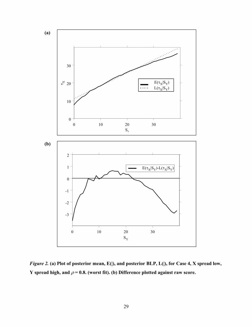
were 13.2, 14.8, and 14.9, respectively. Figure 2 shows both the conditional expectation and the

BLP for Case 4 � = 0.80, and we see substantial curvilinearity in the conditional expectation.

The “bend” gets stronger the more correlated the two tests become, and it is related to the

difference in the levels of difficulty of the two tests and not to the lack of a perfect correlation

27

between the abilities they measure. For comparison, we also did Case 1 (X spread and Y spread)

for � = 0.99, and instead of going up, 1,000 2IGk went down to 1.8 from 6.0 for � = 0.80.

While the values of the k2 factors indicate that, for these examples at least, the linear

approximation to the posterior mean by the BLP is quite good, our second approach includes two

graphs (see Figures 1 and 2) that show what the posterior means and the BLP look like as

functions of the conditioning score value. We only show the graphs that correspond to the largest

and smallest values of the k2-factors in our original study design.

The BLP is an approximation to the conditional expectation because Theorem A, part (b)

and Theorem B, part (d) in the appendices show that, averaged over the score distribution, both

L(�X |SX) and E(�X |SX) have the same value (this is also true for L(�X |SY) and E(�X |SY)). Hence,

there can be no constant bias between the approximation and the target—they must cross as we

see in Figures 1 and 2. Our conclusion is that the BLP is a remarkably good linear approximation

to the posterior mean in the IRT model studied here. This suggests the need for future analyses

along these lines for more complicated IRT models.

How good is H as an approximation to the loss of precision that arises through the use of

indirect prediction? First of all, there were, to two decimal values, virtually no differences

between the values of H computed using (51) and one where the value of k2 is set to 0. This

finding is not surprising in light of the small values of k2 that emerged in our study, and it

suggests analyses of H that ignore k2 probably give useful results in many situations. This is a

useful topic for future research.

Figure 3 gives typical examples of the posterior variances for direct and indirect

prediction. It shows a curvilinear relationship between the posterior variance and the

conditioning test score. This curvilinear relationship is predicted from the simple beta-binomial

model (Gelman et al. 1995, p. 477), which is a special case of the Rasch IRT models used here.

Comparing the two graphs, we see that the posterior standard deviations for direct prediction are

smaller than those for indirect prediction, which is exactly what the inflation factor H is

attempting to measure. To see how well H does this, we computed the average ratios of the

posterior standard deviations at each conditioning score point, indirect divided by direct, and

then averaged the results over the score points. If H is to be a useful average measure, it needs to

reflect the average amount by which the posterior standard deviation is increased when we move

from direct to indirect prediction.

28

(a)

(b)

Figure 1. (a) Plot of posterior mean, E(|), and posterior BLP, L(|), for Case 3, X peaked, Y

spread, with � = 0.8. (best fit). (b) Difference plotted against raw score.

0

10

20

30

40�

X

0 10 20 30 40SY

E(�X|SY)L(�X|SY)

0 10 20 30SY

-3

-2

-1

0

1

2

E(�X|SY)-L(�X|SY)

29

(a)

(b)

Figure 2. (a) Plot of posterior mean, E(|), and posterior BLP, L(|), for Case 4, X spread low,

Y spread high, and � = 0.8. (worst fit). (b) Difference plotted against raw score.

0 10 20 30SY

0

10

20

30�

X

L(�X|SY)E(�X|SY)

0 10 20 30SY

-3

-2

-1

0

1

2

E(�X|SY)-L(�X|SY)

30

(a) (b)

Figure 3. Comparison of conditional standard deviations and their average with the

average predicted by the BLP, for both direct and indirect prediction. (a) Case 1, X spread,

Y spread, � = 0.8. (b) Case 2, X peaked, Y peaked, � = 0.8.

0 10 20 30Observed Test Score

1

2

3

4

5

6

7

8

9

Poste

rior S

D

SD(�X|SY)

E[SD(�X|SY)]SD(�X|SX)

obs M[SD(�X|SY)]

E[SD(�X|SX)]obs M[SD(�X|SX)

0 10 20 30Observed Test Score

1

2

3

4

5

6

7

8

9

Post

erio

r SD

SD(�X|SY)

E[SD(�X|SY)]SD(�X|SX)

obs M[SD(�X|SY)]

E[SD(�X|SX)]obs M[SD(�X|SX)

31

When the two tests are not of the same length (i.e., Case 6), some means of connecting

their score values needs to be worked out to form these ratios of posterior standard deviations.

We simply scored the two tests by the percentage correct and pooled values of the standard

deviations associated with the neighboring scores of the test with the larger number of score

values. We used (64) to form the target ratios.

Target ratios = Var( | ) { }Var( | )

X YX

s X X

S s P S sS s

�

�

�

��

�

. (64)

The values of the target ratios and the values of H are given in Table 5.

Table 5

Average Values of Target Ratios and H

Case X Y H � = .8

H � = .5

Mean Ratio � = .8

Mean Ratio � = .5

5 Spread 20 Spread 20 1.49 (.04) 1.95 (.05) 1.51 (.04) 1.99 (.02) 1 Spread Spread 1.86 (.03) 2.53 (.03) 1.89 (.03) 2.58 (.04) 6 Spread 40 Spread 20 1.99 (.04) 2.60 (.05) 2.04 (.03) 2.64 (.08) 4 Spread

Low Spread High

1.92 (.03) 2.55 (.03) 1.77 (.03) 2.48 (.03)

2 Peaked Peaked 2.02 (.02) 2.70 (.02) 2.07 (.03) 2.81 (.07) 3 Peaked Spread 2.03 (.02) 2.71 (.03) 2.03 (.03) 2.77 (.06)

Note: Table shows the average values of H and of the average ratios of the target posterior standard deviations for the several simulation conditions in the study. (Standard deviations across the 10 replications are in parentheses.)

Table 5 shows that the H values, while usually smaller than the target values, are quite

close and give exactly the same general type of information about the effect of indirect

prediction relative to direct prediction for the 12 conditions of the simulation study. We regard

this finding as a clear support for further work on the BLP tools we have developed here.

How does indirect prediction increase the imprecision of the prediction of the true score

of the target test, X. Using the H values, we get a clear picture as to what happens when we link a

test that measures a different construct in a different way to a target test in terms of degrading the

accuracy of the prediction of the target true score. For example, in this study the posterior

32

standard deviation is inflated by factors ranging from 49% to 171%, depending on the simulation

condition. As the correlation between the constructs lessens, the inflation factor increases.

Interestingly, the smallest inflation factors arise for the case of the least reliable tests, Case 6.

This may be due to the fact that the least reliable tests have poorer direct prediction to begin with

and thus the least to lose from using indirect test data to predict their true scores. This finding is

worth more investigation than we have reported here.

A Real Data Example. We also examined an example using test data from an

administration of a fifth grade Science assessment in two states in 1998. This assessment

involved both a multiple choice test (MC) with 29 items and a performance task test (PT) that

had a performance task followed by nine questions asking the students to record their

observations and explain them. The PT questions were scored dichotomously using expert

judgement. We will use these two different testing formats as the two tests in our study and use

the PT scores to indirectly predict the true scores on the MC.

Data were available for 1,202 girls and 1,096 boys, and we will use gender as the

subgroup-defining variable, G.

Table 6 shows some raw score (number right) means. According to the raw score means,

the two tests, MC versus PT, reverse the order of the two groups—boys perform better on the

MC (by 1.6% of a standard deviation) and girls better on the PT (by 9.9% of a standard

deviation). We used the Dorans-Holland root-expected-mean-square-difference measure

(REMSD)(Doran & Holland, 2000) to measure the average boy-girl difference between parallel-

linear equating functions linking these two tests. The REMSD is 5.6%, which is of moderate size

compared to the examples in their paper.

We used ConQuest to estimate IRT models for these data. In particular, we wanted to

estimate two different thetas, one for the MC and another one for the PT. We also wanted to

obtain separate bivariate normal ability distributions for boys and girls. In all cases, we fit Rasch

models for the items and bivariate normal distributions for the thetas. We did not want to add an

investigation of DIF to this study, so we estimated common item parameters for both genders.

33

Table 6

Raw Means of Number Right Scores

All Girls Boys Difference Standardized differencea

Multiple choice

16.17 (4.96)

16.13 16.21 -0.08 -1.6%

Performance task

4.73 (2.03)

4.83 4.63 0.20 9.9%

Note: Means of number right scores for the MC and PT for all students and separately for boys and girls. (Standard deviations in parentheses.) a Difference divided by the standard deviation for all, expressed as a percentage.

We did this estimation in two ways. First, we estimated a model for the girls only,

anchored the item parameters for boys to the values obtained for girls, and estimated the boys’

bivariate theta distribution subject to this constraint. Second, we reversed the process and

anchored the item parameters to the values estimated for the boys. The results for both

approaches are given separately and show minor differences. Some evidence showed that the

item parameters were slightly different for the two groups, but we do not think these differences

are large enough to affect the conclusions we reached in this example. Table 7 summarizes

various quantities of interest when the IRT analyses are performed separately for boys and girls

and for the total group. We see very little difference between the two methods of anchoring the

items, so we will comment on it no further. The reliabilities of both tests, the MC and PT, are

slightly higher for boys than for girls. However, the average posterior variances (shown here in

the square root scale) show the opposite trend, with the girls having slightly smaller average

posterior variances for either direct or indirect prediction. The values of k2 are all small and have

virtually no effect on H, the inflation factor. H is larger for boys than for girls, indicating that the

indirect prediction of the true score for the MC from the PT scores inflates the prediction error

more for the boys than it does for the girls.

34

Table 7

IRT Results for the Science Assessment Test Data

Item parameters anchored at values for Girls

Item parameters anchored at values for Boys

Girls Boys All Girls Boys Reliability (MC) .74 .77 .75 .73 .77 Reliability (PT) .56 .61 .58 .55 .60 Square root of E[Var(�X|SX, G)| G]

2.11 2.14 2.13 2.13 2.16

Square root of E[Var(�X|SY, G)| G]

3.41 3.75 3.57 3.38 3.74

2DGk .002 .002 .003 .003 .002

2IGk .006 .007 .005 .012 .004

H (setting k2 = 0) 1.62 1.76 1.67 1.60 1.74 H 1.62 1.76 1.68 1.60 1.74

The values of the EPDD and EPDI values are respectively .023 (2.3%) and .038 (3.8%).

These values indicate that subgroup differences have bigger effects on indirect prediction than

they have for direct prediction. The values of the EPDD and EPDI measures are smaller than the

Dorans-Holland REMSD value of 5.6% given earlier. Since the connection between the two

calculations is mostly by analogy, there is no reason for their values to be equal.

6. Discussion

The general IRT model we have developed here reproduces the main results of CTT in

considerable detail, including CTT models that involve more than one test. In addition, we see

that using the concept of BLP provides us with a version of CTT that does not need to assume

the form of the conditional means and variances is linear or constant and that does not really hold

for test data. Furthermore, our simulation study suggests that BLPs are useful alternatives to the

posterior means of the true scores, at least for the simple model we have examined.

In addition to these general considerations, this approach allows us to successfully

distinguish between direct and indirect true-score prediction in a simple but useful way. For

example, it allows us to compute an index of the loss of information that accompanies the linking

35

of nonparallel tests using true score prediction as the criterion. This is expressed in our index, H,

which can be computed from quantities that are usually available in test-linking studies. In

addition, we can generalize the Kelley formula for predicting a true score from an observed score

so that the formula predicts the true score from a nonparallel test. Our analysis shows that linear

regression gives an appropriate linking function (viewed as a BLP approximation to the posterior

expectation) but that the proper residual standard deviation is not that given by the usual

regression results. This justifies the use of multiple regression to link tests in studies such as

Pashley and Phillips (1993) and Williams, Billeaud, Davis, Thissen, and Sanford (1995).

The oft-stated assertion that “regression is not equating” immediately comes to mind

when we talk about linking in the manner that we have in this paper. We think that our approach

is a useful starting point, but it is not directly about test equating per se. For example, the

symmetry requirement of equating cannot hold for true score prediction as we have defined it

here.

This research suggests several topics that might be worth future investigations. First, it

seems useful to investigate the improvements that could be garnered by use of the best quadratic

predictor rather than the BLP. The departures from linearity shown in Figure 2 suggest that a

quadratic term will fit most of the departure from linearity that the conditional expectation

exhibits there. Since we have only looked at the simplest IRT model, however, it also would be

worthwhile to investigate the value of these ideas in more complex models for which the total

score is not a sufficient statistic. In addition, instead of the constant average variance formula in

computing H, it may be worthwhile to find a quadratic version of this using the beta-binomial as

a starting point.

Another possible use for the BLP and the other quantities is to provide “targets” for the

convergence of complex estimation procedures such as those exploiting Markov Chain Monte

Carlo methods. It is possible that having an easily computed target quantity like the BLP

available could indicate when the samples from the posterior distributions have converged to

reasonable values.

36

References

Bock, R. D., & Mislevy, R. J. (1982). Adaptive EAP estimation in a microcomputer

environment. Applied Psychological Measurement, 6, 431–444.

Dorans, N.,& Holland, P. W. (2000). Population invariance and the equatability of tests: Basic

theory and the linear case. Journal of Educational Measurement, 37, 281–306.

Feuer, M. J., Holland, P. W., Green, B. F., Bertenthal, M. W., & Hemphill, F. C. (1999).

Uncommon measures. Washington, DC: National Academy Press.

Gelman, A., Carlin, J. B., Stern, H. S., & Rubin, D. B. (1995). Bayesian data analysis. London:

Chapman and Hall.

Holland, P. W. (1990). On the sampling theory foundations of item response theory models.

Psychometrika, 55, 577–601.

Kelley, T. L. (1923). Statistical methods. New York: Macmillan.

Lord, F. M., & Novick, M. R. (1968). Statistical theories of mental test scores. Reading, MA:

Addison-Wesley.

Mislevy, R. J., Beaton, A. E., Kaplan, B., & Sheehan, K. M. (1992). Estimating population

characteristics from sparse matrix samples of item responses. Journal of Educational

Measurement, 29, 133–161.

Pashley, P. J., & Phillips, G. W. (1993). Toward world-class standards: A research study linking

national and international assessments. Princeton NJ: Educational Testing Service.

Wainer, H., Vevea, J.L., Camacho, F., Reeve, B.B. III, Rosa, K., Nelson, L., et al. (2001).

Augmented scores—“borrowing strength” to compute scores based on small numbers of

items. In D. Thissen & H. Wainer (Eds.), Test scoring, pp. 343-387. Mahwah, NJ:

Erlbaum.

Williams, V., Billeaud, K., Davis, L. A., Thissen, D., & Sanford, E. E. (1995). Projecting to the

NAEP scale: Results from the North Carolina End-of-Grade testing program (Technical

Report No. 34). Chapel Hill, NC: National Institute of Statistical Science, University of

North Carolina, Chapel Hill.

Wu, M., Adams, R.,& Wilson, M. (1997). ConQuest [Computer software]. Melbourne, Australia:

Australian Council for Educational Research.

37

Appendix A

Some Facts About Conditional Distributions, Means, Variances, and Covariances

We will use U, V, and W to denote random variables defined over P so that we can state

these results more generally than the specific notation we developed in Section 1 for testing

applications. We will also, whenever possible, state results conditionally given a subpopulation,

defined in terms of G, as in Section 1. We will use the notation, E(U| V, G), to denote the

conditional expectation, or mean, of U given the values of V and G, and the notation, Var(U| V,

G), for the corresponding conditional variance. Finally, Cov(U, V |W, G) denotes the conditional

covariance of U and V given W and G. We use P{U = u |V, G} to denote the conditional

probability distribution of U given V and G.

Theorem A: If U, V, and W denote random variables for which all of the following

conditional means, variances, and covariances are well-defined, then the following relationships

always hold:

(a) P{U = u | G} = E[ P{U = u | V, G}|G],

where the outer expectation is averaging P{U = u | V, G} over the conditional distribution

of V given G; this is repeated in parts (b)–(d).

(b) E(U | G) = E[E(U | V, G)| G],

i.e., the appropriate mean of conditional expectation is a (less) conditional expectation.

(c) Var(U | G) = E[Var(U | V, G)| G] + Var[E(U | V, G)| G],

i.e., the mean of the conditional variance plus the variance of the conditional mean, which

is the basis of all “within plus between” decompositions of a variance.

(d) Cov(U, V | G) =

E[Cov(U, V | W, G)| G] + Cov[E(U | W, G), E(V | W, G) | G],

i.e., this is a generalization of partc to covariances.

38

Appendix B

Best Linear Predictors

In this paper we use the idea of a BLP of one random variable by another as a way

around doing the more difficult computations of conditional means and variances. Suppose U

and V are two random variables, then the BLP of U from V is denoted by

L(U| V) = � + �V,

where � and ��are chosen to minimize

E(U – � – �V)2.

Hence a BLP is “best” only in the sense of minimizing the average prediction error. The

BLP may also be put into a form that is similar to the “everything is conditional on G form” used

in Theorem A, by having �G and �G chosen to minimize the quantity: E[(U – � – �V)2| G]. In

this case, we will denote the BLP by L(U |V, G).

The value of the minimized E[(U – � – �V)2 |G] is called the “average prediction error”

and it may be expressed as the average, over V given G, of the “conditional prediction error,”

E[(U – � – �V)2 |V, G]. Below we use a somewhat evocative, but nonstandard, notation for these

prediction error measures. 2

| ,UV G� (V) = E[(U – L(U|V, G))2|V, G], and

2| ,UV G� = E{ 2

| ,UV G� (V)|G} = E{E[(U – L(U|V, G))2|V, G]|G}

= E{[(U – L(U|V, G))2|G}.

Thus, 2| ,UV G� (V) measures how poorly L(U |V, G) predicts U for a given value of V,

while 2| ,UV G� is an average of this prediction error measure over the distribution of V given G. In

this sense, 2| ,UV G� (V) is analogous to the conditional variance of U given V and G while 2

| ,UV G�

is analogous to the (conditional given G) mean of the conditional variance of U given V and G.

It is important to point out that when the conditional expectation function, E(U |V, G) is

linear in V, it is identical to the BLP, L(U |V, G) because the conditional expectation is the best

predictor of any form, linear or nonlinear. In this case, 2| ,UV G� (V) is the conditional variance of

39

U given V and G and 2| ,UV G� is the (conditional given G) mean of the conditional variance of U

given V and G.

Theorem B summarizes some well-known and easily derived facts about the BLP.

Theorem B: If L(U |V, G) = �G��+ �GV is the BLP of U from V, in the sense of

minimizing E[(U – �G � �GV)2 |G], then �G� �G and the average squared prediction error 2| ,UV G�

have these values:

(a) �G = | |GU G V G� � �� ,

(b) �G = ||

|

U GUV G

V G

��

�,

and

(c) 2| ,UV G� = 2 2

| |(1 )U G UV G� �� .

In addition, the BLP has these relationships to the conditional moments of U given V:

(d) E[L(U| V, G)| G] = E[U| G],

i.e., the mean of the BLP is the mean of the predicted variable, U. This parallels Theorem

A, part (b).

(e1) 2| ,UV G� = E[Var(U| V, G)| G] + E[(E(U| V, G) – L(U| V, G))2| G],

= E[Var(U| V, G)| G] + Var[E(U| V, G) – L(U| V, G)| G],

or

(e2) E[Var(U| V, G)| G] = 2| ,UV G� – Var[E(U| V, G) – L(U| V, G)| G].

Part (e1) parallels Theorem A, part (c) in that it is like a “between and within” variance

decomposition. Part (e2) shows how the mean of the conditional variance of U can be expressed

in terms of the average squared prediction error and the variance of the difference between the

BLP and the corresponding conditional expectation.

The quantities given in Theorem B, parts (a) to (c), are exactly the same as the formulas

for the intercept, slope, and residual variance formulas that hold when the conditional

distribution of U given V has a linear conditional expectation function and constant conditional

variance. These conditions hold, for example, when U and V have a joint bivariate normal

distribution. However, the BLP is useful even when the conditional mean function is not linear

40

or when the conditional variance function is not constant, as is the case in most of the IRT

applications we consider here. Parts (d), (e1), and (e2) of Theorem B show the connection

between the BLP and the conditional mean and variance of the joint distribution of U and V.

These last three results motivate our notation of L(U| V, G) to mimic the conditional expectation

notation, E(U| V, G).