classical latent variable models for medical research · classical latent variable models for...
TRANSCRIPT
Statistical Methods in Medical Research 2008; 17: 5–32
Classical latent variable modelsfor medical researchSophia Rabe-Hesketh Graduate School of Education and Graduate Group in Biostatistics,University of California, Berkeley, USA and Institute of Education, University of London,London, UK and Anders Skrondal Department of Statistics and The Methodology Institute,London School of Economics, London, UK and Division of Epidemiology, Norwegian Instituteof Public Health, Oslo, Norway
Latent variable models are commonly used in medical statistics, although often not referred to under thisname. In this paper we describe classical latent variable models such as factor analysis, item responsetheory, latent class models and structural equation models. Their usefulness in medical research is demon-strated using real data. Examples include measurement of forced expiratory flow, measurement of physicaldisability, diagnosis of myocardial infarction and modelling the determinants of clients’ satisfaction withcounsellors’ interviews.
1 Introduction
Latent variable modelling has become increasingly popular in medical research. By latentvariable model we mean any model that includes unobserved random variables whichcan alternatively be thought of as random parameters. Examples include factor, itemresponse, latent class, structural equation, mixed effects and frailty models.
Areas of application include longitudinal analysis1, survival analysis2, meta-analysis3,disease mapping4, biometrical genetics5, measurement of constructs such as qualityof life6, diagnostic testing7, capture–recapture models8, covariate measurement errormodels9 and joint models for longitudinal data and dropout.10
Starting at the beginning of the 20th century, ground breaking work on latent vari-able modelling took place in psychometrics.11–13 The utility of these models in medicalresearch has only quite recently been recognized and it is perhaps not surprising that med-ical statisticians tend to be unaware of the early, and indeed contemporary, psychometricliterature.
In this paper we review classical latent variable models, namely common factor mod-els and structural equation models (with continuous observed and continuous latent
Address for correspondence: Sophia Rabe-Hesketh, 3659 Tolman Hall, University of California, Berkeley,CA 94720-1670, USA. E-mail: [email protected]
© 2008 SAGE Publications 10.1177/0962280207081236Los Angeles, London, New Delhi and Singapore
© 2008 SAGE Publications. All rights reserved. Not for commercial use or unauthorized distribution. at UNIV CALIFORNIA BERKELEY LIB on June 5, 2008 http://smm.sagepub.comDownloaded from
6 S Rabe-Hesketh and A Skrondal
variables), item response models (with categorical observed and continuous latent vari-ables) and latent class models (with categorical observed and categorical latent variables)and demonstrate their usefulness in medical research using real data. We focus on clas-sical latent variable models for several reasons: 1) the classical models can be fruitfullyapplied in medical research without modifications, 2) familiarity with classical latentvariable models can help standardize terminology and thereby facilitate communica-tion and perhaps more importantly, prevent misguided applications, 3) familiarity canreduce the risk of ‘reinventing the wheel’ and wasting resources on developing programsfor problems that can be readily handled by standard software and 4) the classical modelsare important because they typically serve as building blocks for more advanced latentvariable models. Although we consider mixed effects models14,15 to be latent variablemodels, we do not include them here since they are so well known in medical statistics.
The plan of the paper is as follows. In Sections 2–5, we introduce classical latentvariable models. In each of these sections we present examples using real data, mentioncommon uses of the models in medical research and recommend further reading. Finally,we close the paper with some remarks regarding recent developments. A brief overviewof useful software for latent variable modelling is given in an appendix.
2 Common factor models
2.1 Unidimensional factor modelsConsider j = 1, . . . , N independent subjects. The classical measurement model from
psychometric test theory,16 also called the parallel measurement model, assumes thatrepeated measurements yij of the same true score β + ηj for subject j are conditionallyindependent given ηj with conditional expectation β + ηj,
yij = β + ηj + εij, E(ηj) = 0, E(εij) = 0, Cov(ηj, εij) = 0,
where β is the population mean true score, ηj are independently distributed randomdeviations of subjects’ true scores from the population mean with variance ψ andεij are independently distributed measurement errors with constant variance θ . Thecorresponding standard deviation
√θ is called the standard error of measurement.
This model is appropriate if the repeated measurements are exchangeable. However,if yij are not merely replicates, but measurements using different instruments or ratersi, it is likely that the instruments or raters use different scale origins and units. Thissituation is accommodated by the so-called congeneric measurement model17
yij = βi + λiηj + εij, (1)
where the measure-specific mean, scale and measurement error variance are given byβi, λi and θii, respectively. The reliability ρi, the fraction of true score variance to total
© 2008 SAGE Publications. All rights reserved. Not for commercial use or unauthorized distribution. at UNIV CALIFORNIA BERKELEY LIB on June 5, 2008 http://smm.sagepub.comDownloaded from
Classical latent variable models 7
variance, for a particular instrument i becomes
ρi ≡ (λi)2ψ
(λi)2ψ + θii
Without any parameter constraints the model is not identified (several sets of param-eter values can produce the same probability distribution) because multiplying thestandard deviation
√ψ of the common factor by an arbitrary positive constant can
be counteracted by dividing all factor loadings by the same constant. Identification isachieved either by anchoring, where the first factor loading is fixed to one, λ1 = 1, or byfactor standardization, where the factor variance is set to one, ψ = 1.
There are several important special cases of the congeneric measurement model. Theessentially tau-equivalent measurement model is obtained if the scales of the instrumentsare identical λi = 1, the tau-equivalent measurement model if λi = 1 and the originsare identical βi = β, and the parallel measurement model if λi = 1, βi = β and themeasurement error variances are identical θii = θ .
It should be noted that the congeneric measurement model is a unidimensional factormodel with factor loading λi, common factor ηj and unique factors εij for indicatorsyij. Spearman11 introduced this model, arguing that intelligence is composed of a gen-eral factor, common to all subdomains such as mathematics, music, etc., and specificfactors for each of the subdomains. The common factor can represent any hypotheti-cal construct, a concept that cannot even in principle be directly observed, intelligenceand depression18 being prominent examples. In this case the measures i are typicallyquestions or items of a questionnaire or structured interview.
The expectation of the vector of responses yj = (y1j, . . . , ynj)′ for subject j is
β = (β1, . . . , βn)′ and the model-implied covariance matrix, called the factor structure,
becomes� ≡ Cov(yj) = �ψ�′ + �, (2)
where � = (λ1, . . . , λn)′ and � is a diagonal matrix with the θii on the diagonal.
2.1.1 Estimation, goodness-of-fit and factor scoringFor maximum likelihood estimation, it is invariably assumed that the common and
unique factors are normally distributed, implying a multivariate normal distribution foryj. Replacing the β in the likelihood by their maximum likelihood estimates, the samplemeans y·, gives a profile likelihood
lM(�, ψ , �) = |2π�|− n2 exp(−1
2
N∑
j=1
(yj − y·)′�−1(yj − y·)
In the case of complete data, the empirical covariance matrix S of yj is the sufficientstatistic for the parameters. It can be shown19 that instead of maximizing the likelihood
© 2008 SAGE Publications. All rights reserved. Not for commercial use or unauthorized distribution. at UNIV CALIFORNIA BERKELEY LIB on June 5, 2008 http://smm.sagepub.comDownloaded from

8 S Rabe-Hesketh and A Skrondal
we can equivalently minimize the fitting function
FML = log |�| + tr(S�−1) − log |S| − n, (3)
with respect to the unknown free parameters. The fitting function is non-negative andzero only if there is a perfect fit in the sense that the fitted � equals S. When there aremissing data, the ‘case-wise’ likelihood is maximized giving consistent estimates if dataare missing at random (MAR).20
Treating the unstructured covariance matrix as the saturated model, a likelihood ratiogoodness-of-fit test can be used. Under the null hypothesis that the restricted model ofinterest is correct (and suitable regularity conditions), the likelihood ratio statistic ordeviance has a chi-square distribution with n(n + 1)/2 − p degrees of freedom, wherep is the number of parameters in the restricted model (after eliminating the intercepts),equal to 2n in the congeneric measurement model. Since most parsimonious and henceappealing models are rejected in large samples, more than a hundred goodness-of-fitindices21 have been proposed that are relatively insensitive to sample size. Some of theseindices (e.g., root mean square error of approximation (RMSEA)22) are based on acomparison with the saturated model, but most (e.g., comparative fit index (CFI)23,Tucker-Lewis index (TLI)24) are based on a comparison with the unrealistic null modelof uncorrelated items, and are thus analogous to the coefficient of determination inlinear regression. Arbitrarily, fit is typically considered ‘good’ if the RMSEA is below0.05 and the CFI and TLI are above 0.90.
Often the purpose of factor modelling is to investigate the measurement properties ofdifferent raters, instruments or items i by comparing the fit of congeneric, tau-equivalentand parallel models and estimating reliabilities. Another purpose is measurement itself,that is assigning factor scores to individual subjects j after estimating the model. Themost common approach is the so-called regression method,
ηj = ψ�′�
−1( yj − β).
This can motivated as the expectation of the posterior distribution of the commonfactor given the observed responses with parameter estimates plugged in, known as theempirical Bayes predictor or shrinkage estimator in statistics. An alternative approachis the Bartlett method,
ηj = (�′�
−1�)−1�
′�
−1( yj − β),
which maximizes the likelihood of the responses given the common factor withparameter estimates plugged in.
In the classical measurement model, factor scores using either the regression or Bartlettmethod are perfectly correlated with the simple sum score
∑i yij. For this model, Cron-
bach’s α, a commonly used measure of internal consistency of a scale, can be interpretedas the reliability of the sum score.
2.1.2 Example: Forced expiratory flowIn the Health Survey of England 2004 (National Centre for Social Research and
University College London, Department of Epidemiology and Public Health25), a sam-ple of children between 7 and 15 years of age had their lung function assessed using a
© 2008 SAGE Publications. All rights reserved. Not for commercial use or unauthorized distribution. at UNIV CALIFORNIA BERKELEY LIB on June 5, 2008 http://smm.sagepub.comDownloaded from

Classical latent variable models 9
Vitalograph Micro Spirometer. Here, we consider forced expiratory flow which was mea-sured five times for 89 of the children. The nurse also recorded at each occasion whetheror not the technique used was satisfactory. If not satisfactory, we treat the measurementas missing.
Table 1 shows maximum likelihood estimates for the classical, essentially tau-equivalent, tau-equivalent and congeneric measurement models. Using likelihood ratiotests at the 5% level, the essentially tau-equivalent measurement model is selected. Thismodel also has the best fit indices, but the RMSEA is larger than the desired 0.05. Notethat the estimated mean increases over time are consistent with a practice effect and thatthe estimated measurement error variance is very low at the third measurement. Theestimated reliabilities range between 0.82 at the first measurement and 0.96 at the third.
2.2 Multidimensional factor modelsHypothetical constructs are often multidimensional, comprising several related
aspects. An example is fatigue, for which Nisenbaum et al.26 argue that, there are threecorrelated aspects or common factors defined as ‘fatigue-mood-cognition’, ‘flu-type’,and ‘visual-impairment’.
Table 1 Forced expiratory flow–Maximum likelihood estimates for measurement models
Parallel/ EssentiallyClassical Tau-equivalent Tau-equivalent Congeneric
Est (SE) Est (SE) Est (SE) Est (SE)
Interceptsβ1 257 (11) 261 (11) 231 (12) 232 (12)β2 257 (11) 261 (11) 250 (12) 250 (12)β3 257 (11) 261 (11) 262 (11) 263 (11)β4 257 (11) 261 (11) 271 (12) 271 (12)β5 257 (11) 261 (11) 272 (12) 272 (12)
Factor loadingsλ1 1 1 1 1λ2 1 1 1 1.1 (0.08)λ3 1 1 1 1.1 (0.07)λ4 1 1 1 1.2 (0.08)λ5 1 1 1 1.1 (0.08)
Factor varianceψ 10500 (1638) 10773 (1660) 10934 (1685) 9024 (1711)
Meas. errorvariances
θ11 1772 (143) 3519 (616) 2429 (440) 2372 (423)θ22 1772 (143) 1743 (325) 1527 (289) 1548 (295)θ33 1772 (143) 386 (144) 435 (141) 445 (142)θ44 1772 (143) 1302 (259) 1193 (239) 1125 (237)θ55 1772 (143) 1958 (364) 1818 (336) 1783 (335)
Goodness-of-fitstatistics
Log-likelihood −2182.7 −2162.8 −2142.7 −2140.4Deviance (d.f.) 106.97 (17) 67.05 (13) 26.95 (9) 22.35 (5)CFI 0.85 0.91 0.97 0.97TLI 0.91 0.93 0.97 0.94RMSEA 0.24 0.22 0.15 0.20
© 2008 SAGE Publications. All rights reserved. Not for commercial use or unauthorized distribution. at UNIV CALIFORNIA BERKELEY LIB on June 5, 2008 http://smm.sagepub.comDownloaded from

10 S Rabe-Hesketh and A Skrondal
Denoting the common factors as ηj = (η1j, η2j, . . . , ηmj)′, the multidimensional
common factor model can be written as
yj = β + �ηj + εj, (4)
where � is now a n × m matrix of factor loadings with element pertaining to item i andlatent variable l denoted λil and εj a vector of unique factors. We define � ≡ Cov(ηj) andassume that E(ηj) = 0, E(εj) = 0, and Cov(ηj, εj) = 0. Note that the structure of themodel is similar to a linear mixed model where � is replaced by a covariate matrix Zj.27
The results presented in Section 2.1 from Equation (2) apply also to the multidimensionalfactor model after substituting � for ψ .
It is important to distinguish between two approaches to common factor modelling;exploratory factor analysis and confirmatory factor analysis (CFA).
Exploratory factor analysisExploratory factor analysis (EFA)12,13 is an inductive approach for ‘discovering’ the
number of common factors and estimating the model parameters, imposing a mini-mal number of constraints for identification. The standard identifying constraints arethat � = I, and that � and �′�−1� are both diagonal. Although mathematicallyconvenient, the one-size-fits-all parameter restrictions imposed in EFA, particularly thespecification of uncorrelated common factors, are often not meaningful from a subjectmatter point of view.
Methods of estimation include maximum likelihood using the fitting function in (3)and principal axis factoring. However, due to confusion between factor analysis andprincipal component analysis, the latter is often used. In a second step, the restrictionsimposed for identification are relaxed by rotating the factors to achieve equivalent modelsthat are more interpretable by different criteria, such as varimax.28
Confirmatory factor analysisIn CFA,17,29 restrictions are imposed based on substantive theory or research design.
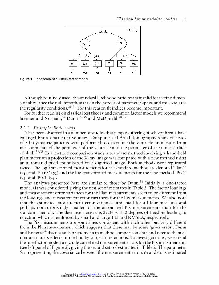
This approach was illustrated for the unidimensional factor model in Section 2.1.2. Inthe multidimensional case an important example of a restricted model is the indepen-dent clusters or sets of congeneric measures model where � has many elements set tozero such that each indicator measures one and only one factor. Such a configurationmakes sense if one set of indicators is designed to measure one factor and another setof indicators to measure another factor. A path diagram of a two-factor independentclusters model with three variables measuring each factor is given in Figure 1. Circlesrepresent latent variables, rectangles represent observed variables, arrows connectingcircles and/or rectangles represent regressions and short arrows pointing at circles orrectangles represent residuals. Curved double-headed arrows connecting two variablesindicate that they are correlated.
For identification the scales of the common factors are fixed either by factor stan-dardization or by anchoring. Elements of εj may be correlated, but special care mustbe exercised in this case to ensure that the model is identified. It is typically assumedthat the common and unique factors have multivariate normal distributions to allowmaximum likelihood estimation as outlined in Section 2.1.
© 2008 SAGE Publications. All rights reserved. Not for commercial use or unauthorized distribution. at UNIV CALIFORNIA BERKELEY LIB on June 5, 2008 http://smm.sagepub.comDownloaded from
Classical latent variable models 11
Figure 1 Independent clusters factor model.
Although routinely used, the standard likelihood ratio test is invalid for testing dimen-sionality since the null hypothesis is on the border of parameter space and thus violatesthe regularity conditions.30,31 For this reason fit indices become important.
For further reading on classical test theory and common factor models we recommendStreiner and Norman,32 Dunn33–36 and McDonald.28,37
2.2.1 Example: Brain scansIt has been observed in a number of studies that people suffering of schizophrenia have
enlarged brain ventricular volumes. Computerized Axial Tomography scans of headsof 50 psychiatric patients were performed to determine the ventricle-brain ratio frommeasurements of the perimeter of the ventricle and the perimeter of the inner surfaceof skull.36,38 In a method comparison study a standard method involving a hand-heldplanimeter on a projection of the X-ray image was compared with a new method usingan automated pixel count based on a digitized image. Both methods were replicatedtwice. The log-transformed measurements for the standard method are denoted ‘Plan1’(y1) and ‘Plan3’ (y2) and the log-transformed measurements for the new method ‘Pix1’(y3) and ‘Pix3’ (y4).
The analyses presented here are similar to those by Dunn.36 Initially, a one-factormodel (1) was considered giving the first set of estimates in Table 2. The factor loadingsand measurement error variances for the Plan measurements seem to be different fromthe loadings and measurement error variances for the Pix measurements. We also notethat the estimated measurement error variances are small for all four measures andperhaps not surprisingly, smaller for the automated Pix measurements than for thestandard method. The deviance statistic is 29.36 with 2 degrees of freedom leading torejection which is reinforced by small and large TLI and RMSEA, respectively.
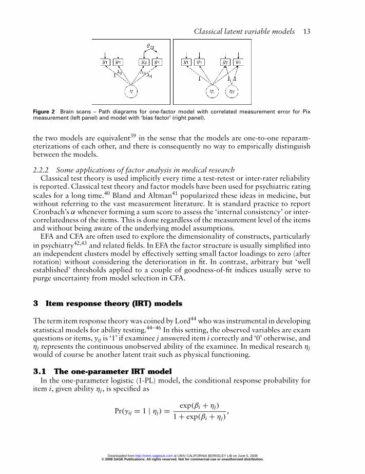
The Pix measurements are sometimes consistent with each other but very differentfrom the Plan measurement which suggests that there may be some ‘gross error’. Dunnand Roberts34 discuss such phenomena in method comparison data and refer to them asrandom matrix effects or method by subject interactions. To investigate this, we extendthe one-factor model to include correlated measurement errors for the Pix measurements(see left panel of Figure 2), giving the second sets of estimates in Table 2. The parameterθ43, representing the covariance between the measurement errors ε3 and ε4, is estimated
© 2008 SAGE Publications. All rights reserved. Not for commercial use or unauthorized distribution. at UNIV CALIFORNIA BERKELEY LIB on June 5, 2008 http://smm.sagepub.comDownloaded from

12 S Rabe-Hesketh and A Skrondal
Table 2 Brain scans – Maximum likelihood estimates (with standard errors) for common factor models
One-factor
One-factor Corr. meas. errors Two-factor
Intercepts
β1 [Plan1] 1.862 (0.056) 1.862 (0.056) 1.862 (0.056)β2 [Plan3] 1.711 (0.061) 1.711 (0.061) 1.711 (0.061)β3 [Pix1] 1.402 (0.073) 1.402 (0.073) 1.402 (0.073)β4 [Pix3] 1.413 (0.074) 1.413 (0.074) 1.413 (0.074)
Factor loadings Factor 1 Factor 2
λ1 [Plan1] 1 – 1 – 0 – 0 –λ2 [Plan3] 1.349 (0.315) 1.377 (0.208) 1.377 (0.208) 0 –λ3 [Pix1] 2.186 (0.423) 1.213 (0.208) 1.213 (0.208) 1 –λ4 [Pix3] 2.197 (0.425) 1.209 (0.210) 1.209 (0.210) 1 –
Factor variances
ψ11 0.056 (0.024) 0.098 (0.031) 0.098 (0.031)ψ22 0.123 (0.029)ψ21 0 –
Measurement error variance
θ11 [Plan1] 0.103 (0.021) 0.060 (0.016) 0.060 (0.016)θ22 [Plan3] 0.086 (0.017) 0.001 (0.019) 0.001 (0.019)θ33 [Pix1] 0.001 (0.003) 0.122 (0.029) a−0.001 (0.003)θ44 [Pix3] 0.002 (0.003) 0.127 (0.029) 0.004 (0.003)
Measurement error covariance
θ43 [Pix1], [Pix3] 0.123 (0.029)
Goodness-of-fit statistics
Log-likelihood 11.56 24.95 24.95Deviance (d.f.) 29.36 (2) 2.57 (1) 2.57 (1)CFI 0.91 1.00 1.00TLI 0.73 0.97 0.97RMSEA 0.52 0.18 0.18
aHeywood case
as 0.123, corresponding to an extremely high measurement error correlation of 0.988.Interestingly, the measurement error variances are now much larger for the Pix measure-ments than for the Plan measurements. The deviance statistic for this model is 2.57 with1 degree of freedom, giving a P-value of 0.10. Although the RMSEA remains somewhathigh, the CFI and TLI are now very satisfactory. Thus, it seems reasonable to retain themeasurement model with correlated measurement errors for the Pix measurements.
Another way of capturing the notion of gross error is to introduce a ‘bias factor’ η2jwhich induces extra dependence among the Pix measurements. The bias factor has factorloadings of one for the two Pix measurements and zero for the two Plan measurementsand is uncorrelated with the original factor (see right panel of Figure 2). Maximum like-lihood estimates with standard errors for this model are presented in the last columns ofTable 2. Note that the estimated measurement error variance for [Pix1] is inadmissiblesince it is negative, a so-called Heywood case, which casts some doubt on the validity ofthis specification. Interestingly, the deviance statistic for this model is identical to thatfor the measurement model with correlated measurement errors. It can be shown that
© 2008 SAGE Publications. All rights reserved. Not for commercial use or unauthorized distribution. at UNIV CALIFORNIA BERKELEY LIB on June 5, 2008 http://smm.sagepub.comDownloaded from
Classical latent variable models 13
Figure 2 Brain scans – Path diagrams for one-factor model with correlated measurement error for Pixmeasurement (left panel) and model with ‘bias factor’ (right panel).
the two models are equivalent39 in the sense that the models are one-to-one reparam-eterizations of each other, and there is consequently no way to empirically distinguishbetween the models.
2.2.2 Some applications of factor analysis in medical researchClassical test theory is used implicitly every time a test-retest or inter-rater reliability
is reported. Classical test theory and factor models have been used for psychiatric ratingscales for a long time.40 Bland and Altman41 popularized these ideas in medicine, butwithout referring to the vast measurement literature. It is standard practice to reportCronbach’s α whenever forming a sum score to assess the ‘internal consistency’ or inter-correlatedness of the items. This is done regardless of the measurement level of the itemsand without being aware of the underlying model assumptions.
EFA and CFA are often used to explore the dimensionality of constructs, particularlyin psychiatry42,43 and related fields. In EFA the factor structure is usually simplified intoan independent clusters model by effectively setting small factor loadings to zero (afterrotation) without considering the deterioration in fit. In contrast, arbitrary but ‘wellestablished’ thresholds applied to a couple of goodness-of-fit indices usually serve topurge uncertainty from model selection in CFA.
3 Item response theory (IRT) models
The term item response theory was coined by Lord44 who was instrumental in developingstatistical models for ability testing.44–46 In this setting, the observed variables are examquestions or items, yij is ‘1’ if examinee j answered item i correctly and ‘0’ otherwise, andηj represents the continuous unobserved ability of the examinee. In medical research ηjwould of course be another latent trait such as physical functioning.
3.1 The one-parameter IRT modelIn the one-parameter logistic (1-PL) model, the conditional response probability for
item i, given ability ηj, is specified as
Pr(yij = 1 | ηj) = exp(βi + ηj)
1 + exp(βi + ηj),
© 2008 SAGE Publications. All rights reserved. Not for commercial use or unauthorized distribution. at UNIV CALIFORNIA BERKELEY LIB on June 5, 2008 http://smm.sagepub.comDownloaded from

14 S Rabe-Hesketh and A Skrondal
where the responses are assumed to be conditionally independent given ability ηj, aproperty often called local independence. This model is called a one–parameter modelbecause there is one parameter, the item difficulty −βi, for each item.
Ability ηj can either be treated as a latent random variable or as an unknown fixedparameter, giving the so-called Rasch model.47 However, estimating the ‘incidentalparameters’ ηj jointly with the ‘structural parameters’ β produces inconsistent estima-tors for β, known as the incidental parameter problem.48 Inference can instead be basedon the conditional likelihood49,50 constructed by conditioning on the sufficient statisticfor ηj, which is the sum score
∑ni=1 yij. This conditional logistic regression approach is
also commonly used in matched case control studies.51
Alternatively, if ηj is viewed as a random variable, typically with ηj ∼ N(0, ψ), infer-ence can be based on the marginal likelihood obtained by integrating out the latentvariable
lM(β, ψ) =N∏
j=1
Pr(yj; β, ψ) =N∏
j=1
∫ ∞
−∞
n∏
i=1
Pr(yij | ηj) g(ηj; ψ) dηj
=N∏
j=1
∫ ∞
−∞
n∏
i=1
exp(βi + ηj)yij
1 + exp(βi + ηj)g(ηj; ψ) dηj,
where − β is the vector of item difficulties and g(·; ψ) is the normal density with zeromean and variance ψ .
An appealing feature of one-parameter models is that items and examinees can beplaced on a common scale (according to the difficulty and ability parameters) so thatthe probability of a correct response depends only on the amount ηj − (−βi) by whichthe examinee’s position exceeds the item’s position. Differences in difficulty betweenitems are the same for all examinees, and differences in abilities of two examinees arethe same for all items, a property called specific objectivity by Rasch.
One of the main purposes of item response modelling is to derive scores from the itemresponses. The most common approach is to use the expectation of the posterior distri-bution of ηj given yj with parameter estimates plugged in. This empirical Bayes approachis analogous to the regression method for common factor models and is referred to asexpected a posterior (EAP) scoring in IRT.
3.1.1 Example: Physical functioningThe 1996 Health Survey for England (Joint Health Surveys Unit of Social and Com-
munity Planning Research and University College London52) administered the PhysicalFunctioning PF-10 subscale of the SF-36 Health Survey53 to adults aged 16 and above.The 15592 respondents were asked:
‘The following items are about activities you might do during a typical day. Does yourhealth now limit you in these activities? If so, how much?’
1) Vigorous activities: Vigorous activities, such as running, lifting heavy objects,participating in strenuous sports
© 2008 SAGE Publications. All rights reserved. Not for commercial use or unauthorized distribution. at UNIV CALIFORNIA BERKELEY LIB on June 5, 2008 http://smm.sagepub.comDownloaded from
Classical latent variable models 15
2) Moderate activities: Moderate activities, such as moving a table, pushing avacuum cleaner, bowling or playing golf
3) Lift/Carry: Lifting or carrying groceries4) Several stairs: Climbing several flights of stairs5) One flight stairs: Climbing one flight of stairs6) Bend/Kneel/Stoop: Bending, kneeling, or stooping7) Walk more mile: Walking more than a mile8) Walk several blocks: Walking several blocks9) Walk one block: Walking one block
10) Bathing/Dressing: Bathing or dressing yourself
The possible responses to these questions are ‘yes, limited a lot’, ‘yes, limited a little’ and‘no, not limited at all’. Here we analyse the dichotomous indicator for not being limitedat all. Then −βi can be interpreted as the difficulty of activity i and ηj as the physicalfunctioning of subject j.
The ten most frequent response patterns and their frequencies are shown in the firsttwo columns of Table 3. Note that about a third of subjects are not limited at all in anyof the activities whereas 6% are limited in all activities. Using conditional maximumlikelihood (CML) estimation with the identifying constraint β1 = 0 gives the difficultyestimates shown under ‘CML’ in Table 4.
For marginal maximum likelihood estimation it seems unrealistic to assume a normaldistribution for physical functioning since such a large proportion of people is not limitedat all on any of the items. We therefore leave the physical functioning distribution unspec-ified using so-called nonparametric maximum likelihood (NPML) estimation.54–58 TheNPML estimator of the latent variable distribution is discrete with number of mass-points determined to maximize the marginal likelihood. Here six points appeared to beneeded but convergence was not achieved, so we present the discrete five-point solutioninstead.
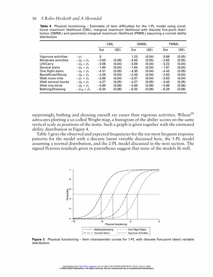
Figure 3 shows the item characteristic curves, the probabilities of not being limitedat all as a function of physical functioning, for four of the items. The value of physi-cal functioning corresponding to a probability of 0.5 is the difficulty of the task. Not
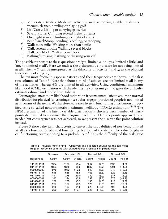
Table 3 Physical functioning – Observed and expected counts for the ten mostfrequent response patterns with signed Pearson residuals in parentheses
Observed Discrete 1-PL Normal 1-PL Normal 2-PL
Responses Count Count (Resid) Count (Resid) Count (Resid)
1111111111 5384 5137 (3.4) 5217 (2.3) 5036 (4.9)0111111111 1884 1670 (5.2) 1632 (6.2) 2091 (−4.5)0000000000 970 1052 (−2.5) 813 (5.5) 978 (−0.3)0110111111 646 518 (5.6) 463 (8.5) 529 (5.1)0111101111 441 275 (10.0) 240 (13.0) 347 (5.0)0000000001 343 294 (2.9) 298 (2.6) 376 (−1.7)0110101111 252 205 (3.3) 190 (4.5) 218 (2.3)0110110111 237 137 (8.5) 126 (9.9) 123 (10.3)0000000011 220 197 (1.6) 229 (−0.6) 193 (1.9)1110111111 209 264 (−3.4) 228 (−1.3) 309 (−5.7)
© 2008 SAGE Publications. All rights reserved. Not for commercial use or unauthorized distribution. at UNIV CALIFORNIA BERKELEY LIB on June 5, 2008 http://smm.sagepub.comDownloaded from
16 S Rabe-Hesketh and A Skrondal
Table 4 Physical functioning – Estimates of item difficulties for the 1-PL model using condi-tional maximum likelihood (CML), marginal maximum likelihood with discrete five-point distri-bution (DMML) and parametric marginal maximum likelihood (PMML) assuming a normal abilitydistribution
CML DMML PMML
Est (SE) Est (SE) Est (SE)
Vigorous activities −β1 0 1.23 (0.04) 0.86 (0.05)Moderate activities −β2 + β1 −3.50 (0.06) −3.50 (0.05) −3.65 (0.05)Lift/Carry −β3 + β1 −3.06 (0.04) −3.06 (0.04) −3.22 (0.04)Several stairs −β4 + β1 −1.85 (0.04) −1.84 (0.04) −1.97 (0.04)One flight stairs −β5 + β1 −4.31 (0.05) −4.30 (0.04) −4.43 (0.05)Bend/Kneel/Stoop −β6 + β1 −2.48 (0.04) −2.48 (0.04) −2.63 (0.04)Walk more mile −β7 + β1 −2.88 (0.04) −2.87 (0.04) −3.03 (0.04)Walk several blocks −β8 + β1 −4.27 (0.05) −4.27 (0.05) −4.40 (0.05)Walk one block −β9 + β1 −5.68 (0.06) −5.68 (0.06) −5.69 (0.06)Bathing/Dressing −β10 + β1 −6.34 (0.06) −6.35 (0.06) −6.28 (0.06)
surprisingly, bathing and dressing oneself are easier than vigorous activities. Wilson59
advocates plotting a so-called Wright map, a histogram of the ability scores on the samevertical scale as positions of the items. Such a graph is given together with the estimatedability distribution in Figure 4.
Table 3 gives the observed and expected frequencies for the ten most frequent responsepatterns for the model with a discrete latent variable discussed here, the 1-PL modelassuming a normal distribution, and the 2-PL model discussed in the next section. Thesigned Pearson residuals given in parentheses suggest that none of the models fit well.
Figure 3 Physical functioning – Item characteristic curves for 1-PL with discrete five-point latent variabledistribution.
© 2008 SAGE Publications. All rights reserved. Not for commercial use or unauthorized distribution. at UNIV CALIFORNIA BERKELEY LIB on June 5, 2008 http://smm.sagepub.comDownloaded from

Classical latent variable models 17
Figure 4 Physical functioning – Estimated distribution (1-PL with five masspoints), distribution of empiricalBayes scores and difficulties of items.
3.2 Two-parameter IRT modelAlthough the 1-PL model is parsimonious and elegant it often does not fit the data.
A more general model is the two-parameter logistic (2-PL) model
Pr(yij = 1 | ηj) = exp(βi + λiηj)
1 + exp(βi + λiηj),
where the factor loading λi is referred to as the discrimination parameter because itemswith a large λi are better at discriminating between subjects with different abilities.The traditional parametrization of the conditional log-odds βi + λiηj is λi(ηj − bi),where bi = −βi/λi is called the difficulty parameter because the probability of a correctresponse is 0.5 if ηj = bi as in the one-parameter model. The model is called a two-parameter model because there are two parameters for each item, the discriminationand difficulty parameter.
Importantly, a conditional likelihood can no longer be constructed since there is nosufficient statistic for ηj and the marginal likelihood assuming that ηj ∼ N(0, 1) is henceused. Since there is no closed form of the marginal likelihood, Bock and Lieberman60
introduced the use of numerical integration by Gauss–Hermite quadrature. Here, weuse a refinement of this approach called adaptive quadrature.61
For the PF-10 example, item characteristic curves for the 2-PL model, assuming a nor-mal distribution for physical functioning, are shown in Figure 5 for the same four itemsas in Figure 3. For the items shown here, Vigorous Activities is the least discriminating
© 2008 SAGE Publications. All rights reserved. Not for commercial use or unauthorized distribution. at UNIV CALIFORNIA BERKELEY LIB on June 5, 2008 http://smm.sagepub.comDownloaded from

18 S Rabe-Hesketh and A Skrondal
Figure 5 Physical functioning – Item characteristic curves for 2–PL.
whereas One Flight Stairs is the most discriminating. Note that the 2-PL model doesnot share the specific objectivity property of the 1-PL model. An item can be easier thananother item for low abilities but more difficult than the other item for higher abilitiesdue to the item-subject interaction λiηj. This property has caused some psychometri-cians to reject the use of discrimination parameters because they ‘wreak havoc with thelogic and practice of measurement’.62
For dichotomous responses, it is often instructive to formulate models using a latentcontinuous response y∗
ij underlying the dichotomous response with
yij ={
1 if y∗ij > 0
0 otherwise.
Specifying a unidimensional factor model for y∗ij
y∗ij = βi + λiηj + εij, ηj ∼ N(0, ψ), εij ∼ N(0, 1), Cov(ηj, εij) = 0,
leads to the so-called normal-ogive model45,63 for the observed yij,
�−1[Pr(yij = 1 | ηj)] = βi + λiηj
Here �(·) is the cumulative standard normal distribution function and �−1(·) is theprobit link. Replacing the probit link by a logit link yields the 2-PL model which canalso be derived by specifying logistic distributions for the specific factors εij in the latentresponse formulation.
© 2008 SAGE Publications. All rights reserved. Not for commercial use or unauthorized distribution. at UNIV CALIFORNIA BERKELEY LIB on June 5, 2008 http://smm.sagepub.comDownloaded from

Classical latent variable models 19
For ordinal responses, proportional odds and adjacent category logit versions of theIRT models described above have been proposed under the names graded responsemodel64 and partial credit model,65 respectively.
We recommend the books by Hambleton et al. 66 and Embretson and Reise67 forfurther reading on IRT.
3.2.1 Some applications of IRT in medical researchIRT is sometimes used in psychiatry for investigating the measurement properties of
rating scales, for instance for affective disorder68 and depression.69,70 More recentlythere has been a surge of interest in IRT for quality of life and related constructs. Forexample, the 2004 Conference on Outcome Research organized by the US NationalCancer Institute was dedicated to IRT. In 2003 there was a special issue of Quality ofLife Research on the measurement of headache which was dominated by papers usingthe Rasch model.
Papers advocating the use of IRT in health outcome measurement include Revicki andCella71 and Hays et al.72 in Quality of Life Research and Medical Care, respectively,journals that regularly publish papers using IRT. However, the use of IRT for qualityof life has been criticized because items, such as those concerning impairment, may bebetter construed as ‘causing’ quality of life than ‘reflecting’ quality of life.6
Item response models have also been used for other purposes than measurement suchas capture–recapture modelling73 for estimation of prevalences, typical examples beingdiabetes or drug use.
4 Latent class models
4.1 Exploratory latent class modelIn latent class models74,75 both the latent and observed variables are categorical. The
C categories of the latent variable can be thought of as labels c = 1, . . . , C classifyingsubjects into distinct sub-populations. For simplicity, we consider binary response vari-ables yij, i = 1, . . . , n. The conditional response probability for variable i, given latentclass membership c, is given by
Pr(yij = 1 | c) = πi|c, (5)
where πi|c are free parameters and different responses yij and yi′j for the same subject areconditionally independent given class membership. The probability that subject j belongsto latent class c is also a free parameter, denoted πc. The model is called exploratorybecause no restrictions are imposed on either the πi|c or the πc.
The marginal likelihood becomes
lM(π) =N∏
j = 1
Pr(yj; π) =N∏
j = 1
C∑
c = 1
πc
n∏
i = 1
Pr(yij | c) =N∏
j = 1
C∑
c = 1
πc
n∏
i = 1
πyiji|c (1 − πi|c)1−yij ,
where π ′ = (π1, π1|1, . . . , πn|1, . . . , πC, π1|C, . . . , πn|C). It is evident that the latent classmodel is a multivariate finite mixture model with C components.
© 2008 SAGE Publications. All rights reserved. Not for commercial use or unauthorized distribution. at UNIV CALIFORNIA BERKELEY LIB on June 5, 2008 http://smm.sagepub.comDownloaded from

20 S Rabe-Hesketh and A Skrondal
For further reading on latent class models we recommend the book by McCutcheon76
and the survey papers by Clogg77 and Formann and Kohlmann,78 the latter with specialemphasis on applications in medicine.
4.1.1 Example: Diagnosis of myocardial infarctionRindskopf and Rindskopf7 analyse data from a coronary care unit in New York City
where patients were admitted to rule out myocardial infarction (MI) or ‘heart attack’.Each of 94 patients was assessed on four diagnostic criteria rated as 1 = present and0 = abscent:
• [Q-wave]–Q-wave in the ECG• [History]–Classical clinical history• [LDH]–Having a flipped LDH• [CPK]–CPK-MB
The data are shown in Table 5. For clarity we label the classes c = 1 for MI and c = 0for no MI. Then π0 is the probability or ‘prevalence’ of not having MI, which can beparameterized as
logit(π0) = �0,
and π1 = 1 − π0. The conditional response probabilities can be specified as
logit[Pr(yij = 1|c)] = eic
The probabilities Pr(yij = 1|c = 1) represent the sensitivities of the diagnostic tests (theprobabilities of a correct diagnosis for subjects with the illness), whereas 1 − Pr(yij =1|c = 0) represent the specificities (the probabilities of a correct diagnosis for subjectswithout the illness).
Table 5 Diagnosis of myocardial infarction data
[Q-wave] [History] [LDH] [CPK] Observed Expected Probability of MI(i = 1) (i = 2) (i = 3) (i = 4) count count (c = 1)
1 1 1 1 24 21.62 1.0000 1 1 1 5 6.63 0.9921 0 1 1 4 5.70 1.0000 0 1 1 3 1.95 0.8891 1 0 1 3 4.50 1.0000 1 0 1 5 3.26 0.4201 0 0 1 2 1.19 1.0000 0 0 1 7 8.16 0.0441 1 1 0 0 0.00 0.0170 1 1 0 0 0.22 0.0001 0 1 0 0 0.00 0.0010 0 1 0 1 0.89 0.0001 1 0 0 0 0.00 0.0000 1 0 0 7 7.78 0.0001 0 0 0 0 0.00 0.0000 0 0 0 33 32.11 0.000
Source: Rindskopf and Rindskopf (1986).7
© 2008 SAGE Publications. All rights reserved. Not for commercial use or unauthorized distribution. at UNIV CALIFORNIA BERKELEY LIB on June 5, 2008 http://smm.sagepub.comDownloaded from
Classical latent variable models 21
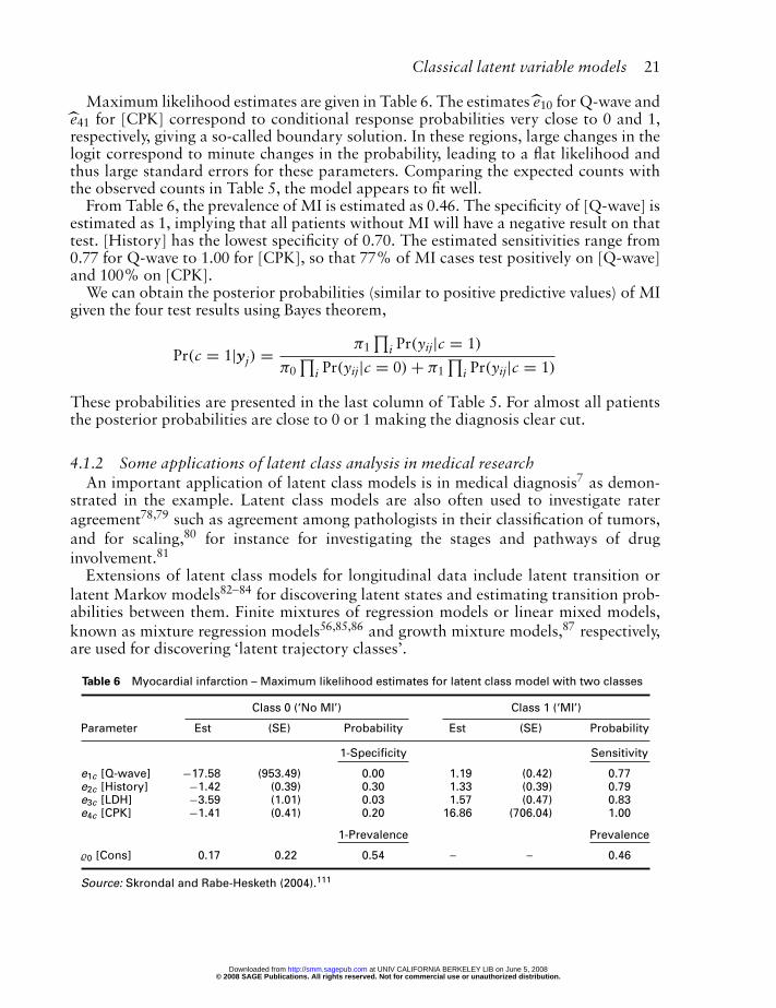
Maximum likelihood estimates are given in Table 6. The estimates e10 for Q-wave ande41 for [CPK] correspond to conditional response probabilities very close to 0 and 1,respectively, giving a so-called boundary solution. In these regions, large changes in thelogit correspond to minute changes in the probability, leading to a flat likelihood andthus large standard errors for these parameters. Comparing the expected counts withthe observed counts in Table 5, the model appears to fit well.
From Table 6, the prevalence of MI is estimated as 0.46. The specificity of [Q-wave] isestimated as 1, implying that all patients without MI will have a negative result on thattest. [History] has the lowest specificity of 0.70. The estimated sensitivities range from0.77 for Q-wave to 1.00 for [CPK], so that 77% of MI cases test positively on [Q-wave]and 100% on [CPK].
We can obtain the posterior probabilities (similar to positive predictive values) of MIgiven the four test results using Bayes theorem,
Pr(c = 1|yj) = π1∏
i Pr(yij|c = 1)
π0∏
i Pr(yij|c = 0) + π1∏
i Pr(yij|c = 1)
These probabilities are presented in the last column of Table 5. For almost all patientsthe posterior probabilities are close to 0 or 1 making the diagnosis clear cut.
4.1.2 Some applications of latent class analysis in medical researchAn important application of latent class models is in medical diagnosis7 as demon-
strated in the example. Latent class models are also often used to investigate rateragreement78,79 such as agreement among pathologists in their classification of tumors,and for scaling,80 for instance for investigating the stages and pathways of druginvolvement.81
Extensions of latent class models for longitudinal data include latent transition orlatent Markov models82–84 for discovering latent states and estimating transition prob-abilities between them. Finite mixtures of regression models or linear mixed models,known as mixture regression models56,85,86 and growth mixture models,87 respectively,are used for discovering ‘latent trajectory classes’.
Table 6 Myocardial infarction – Maximum likelihood estimates for latent class model with two classes
Class 0 (‘No MI’) Class 1 (‘MI’)
Parameter Est (SE) Probability Est (SE) Probability
1-Specificity Sensitivity
e1c [Q-wave] −17.58 (953.49) 0.00 1.19 (0.42) 0.77e2c [History] −1.42 (0.39) 0.30 1.33 (0.39) 0.79e3c [LDH] −3.59 (1.01) 0.03 1.57 (0.47) 0.83e4c [CPK] −1.41 (0.41) 0.20 16.86 (706.04) 1.00
1-Prevalence Prevalence
�0 [Cons] 0.17 0.22 0.54 – – 0.46
Source: Skrondal and Rabe-Hesketh (2004).111
© 2008 SAGE Publications. All rights reserved. Not for commercial use or unauthorized distribution. at UNIV CALIFORNIA BERKELEY LIB on June 5, 2008 http://smm.sagepub.comDownloaded from

22 S Rabe-Hesketh and A Skrondal
5 Structural equation models (SEM) with latent variables
The geneticist Wright88 introduced path analysis for observed variables andJöreskog89–91 combined such models with common factor models to form structuralequation models with latent variables.
There are several ways of parameterizing SEMs with latent variables. The most com-mon is the LISREL parametrization89–91 but we will use a parametrization suggested byMuthén92 here because it turns out to be more convenient for the subsequent application.
The measurement part of the model is the confirmatory factor model (4) specified inSection 2.2. The structural part of the model specifies regressions for the latent variableson other latent and observed variables
ηj = α + Bηj + �xj + ζ j (6)
Here ηj is a vector of latent variables with corresponding lower-triangular parametermatrix B governing the relationships among them, α is a vector of intercepts, � a regres-sion parameter matrix for the regression of the latent variables on the vector of observedcovariates xj, and ζ j is a vector of disturbances. We define � ≡ Cov(ζ j) and assume thatE(ζ j)=0, Cov(xj, ζ j) = 0 and Cov(εj, ζ j) = 0.
Substituting from the structural model into the measurement model, we obtain thereduced form,
yj = β + �(I − B)−1(α + �xj+ζ j) + εj (7)
The mean structure for yj, conditional on the covariates xj, becomes
μj ≡ E( yj|xj) = β + �(I − B)−1(α + �xj),
and the covariance structure of yj, conditional on the covariates, becomes
� ≡ Cov( yj|xj) = �(I − B)−1�[(I − B)−1]′�′ + � (8)
An important special case is the Multiple-Indicator-MultIple-Cause (MIMIC)model93 which imposes the restriction B = I in the structural model (6),
ηj = α + �xj + ζ j
As for common factor models, the marginal likelihood of a SEM can be expressed inclosed form if we assume that ζ j and εj and hence yj, are multivariate normal. Insteadof maximizing the marginal likelihood, we can minimize a fitting function similar to (3),with respect to the unknown free parameters of the SEM.
For further reading on structural equation modelling we recommend the books byLoehlin,94 Bollen95 and Kaplan.96
© 2008 SAGE Publications. All rights reserved. Not for commercial use or unauthorized distribution. at UNIV CALIFORNIA BERKELEY LIB on June 5, 2008 http://smm.sagepub.comDownloaded from

Classical latent variable models 23
5.1 Example: Clients’ satisfaction with counsellors’ interviewsAlwin and Tessler97 and Tessler98 described and analysed data from an experiment to
investigate the determinants of clients’ satisfaction with counsellors’ initial interviews.Three experimental factors were manipulated: 1) ‘Experience (E)’ x1j, clients’ infor-
mation regarding the length of time the counsellor has acted in his professional capacity(no experience versus full-fledged counsellor), 2) ‘Value similarity (VS)’ x2j, the degreeto which the client perceives the counsellor as similar in values and life-style preferences(sharply different philosophy of life versus high communality), and 3) ‘Formality (F)’ x3j,the extent to which the counsellor exercises the maximum level of social distance permit-ted by norms governing a counselling relationship (informal versus formal). Ninety-sixfemale subjects were randomly assigned to the two levels of each of the experimentalfactors in a full factorial design. All subjects were exposed to the same male counsellor.
It was important to assess the degree to which the experimental manipulations hadbeen accurately perceived by the clients. In the measurement part of model, three latentvariables, each corresponding to an experimental factor, were thus considered as ‘manip-ulation checks’: ‘Perceived experience (P-E)’ η1j, measured by the items y1j, y2j and y3j;‘Perceived value similarity (P-VS)’ η2j, measured by the items y4j, y5j and y6j; and ‘Per-ceived formality (P-F)’ η3j, measured by the items y7j, y8j and y9j. An independent clustersconfirmatory factor model (akin to that shown in Figure 1 but with three latent variables)was thus specified for the items, only allowing the items to measure the latent variablesthey were supposed to measure.
Clients’ satisfaction was construed as a two-dimensional latent variable:
• ‘Relationship-centered satisfaction (RS)’ η4j, representing the client’s sense ofcloseness to the counsellor, measured by four items each scored from 0 to 6:– ‘Personalism’ y10,j: A likert item (from ‘agree strongly’ to ‘disagree strongly’)
with question wording ‘I think that the counsellor is one of the nicest personsI’ve ever met’
– ‘Warmth’ y11,j: A semantic differential format (from ‘cold’ to ‘warm’)– ‘Friendliness’ y12,j: A semantic differential format (from ‘friendly’ to
‘unfriendly’)– ‘Concern’ y13,j: A semantic differential format (from ‘unconcerned’ to ‘con-
cerned’)
• ‘Problem-centered satisfaction (PS)’ η5j, representing the client’s perception of thecounsellor’s ability to help, measured by four items each scored from 0 to 6:– ‘Thoroughness’ y14,j: A Likert item (from ‘agree strongly’ to ‘disagree strongly’)
with question wording “The counsellor was very thorough. I was left with thefeeling that nothing important had been overlooked”
– ‘Skillfulness’ y15,j: A semantic differential format (from ‘unskilled’ to ‘skilled’)– ‘Impressiveness’ y16,j: A semantic differential format (from ‘impressive’ to
‘unimpressive’)– ‘Success in bringing clarity to the problem’ y17,j: A Likert item (from ‘agree
strongly’ to ‘disagree strongly’) with question wording ‘I felt that the natureof my problem had been clarified, that is that the counsellor had helped me tounderstand exactly what was troubling me’
© 2008 SAGE Publications. All rights reserved. Not for commercial use or unauthorized distribution. at UNIV CALIFORNIA BERKELEY LIB on June 5, 2008 http://smm.sagepub.comDownloaded from
24 S Rabe-Hesketh and A Skrondal
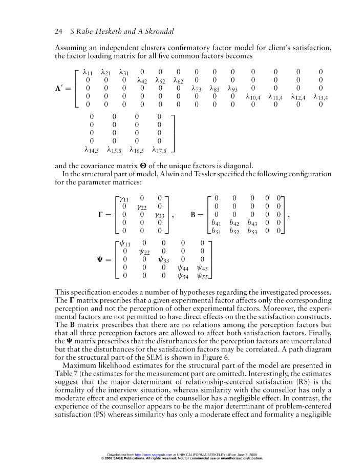
Assuming an independent clusters confirmatory factor model for client’s satisfaction,the factor loading matrix for all five common factors becomes
�′ =
⎡
⎢⎢⎣
λ11 λ21 λ31 0 0 0 0 0 0 0 0 0 00 0 0 λ42 λ52 λ62 0 0 0 0 0 0 00 0 0 0 0 0 λ73 λ83 λ93 0 0 0 00 0 0 0 0 0 0 0 0 λ10,4 λ11,4 λ12,4 λ13,40 0 0 0 0 0 0 0 0 0 0 0 0
0 0 0 00 0 0 00 0 0 00 0 0 0
λ14,5 λ15,5 λ16,5 λ17,5
⎤
⎥⎥⎦
and the covariance matrix � of the unique factors is diagonal.In the structural part of model, Alwin and Tessler specified the following configuration
for the parameter matrices:
� =
⎡
⎢⎢⎣
γ11 0 00 γ22 00 0 γ330 0 00 0 0
⎤
⎥⎥⎦ , B =
⎡
⎢⎢⎣
0 0 0 0 00 0 0 0 00 0 0 0 0
b41 b42 b43 0 0b51 b52 b53 0 0
⎤
⎥⎥⎦ ,
� =
⎡
⎢⎢⎣
ψ11 0 0 0 00 ψ22 0 0 00 0 ψ33 0 00 0 0 ψ44 ψ450 0 0 ψ54 ψ55
⎤
⎥⎥⎦
This specification encodes a number of hypotheses regarding the investigated processes.The � matrix prescribes that a given experimental factor affects only the correspondingperception and not the perception of other experimental factors. Moreover, the experi-mental factors are not permitted to have direct effects on the the satisfaction constructs.The B matrix prescribes that there are no relations among the perception factors butthat all three perception factors are allowed to affect both satisfaction factors. Finally,the � matrix prescribes that the disturbances for the perception factors are uncorrelatedbut that the disturbances for the satisfaction factors may be correlated. A path diagramfor the structural part of the SEM is shown in Figure 6.
Maximum likelihood estimates for the structural part of the model are presented inTable 7 (the estimates for the measurement part are omitted). Interestingly, the estimatessuggest that the major determinant of relationship-centered satisfaction (RS) is theformality of the interview situation, whereas similarity with the counsellor has only amoderate effect and experience of the counsellor has a negligible effect. In contrast, theexperience of the counsellor appears to be the major determinant of problem-centeredsatisfaction (PS) whereas similarity has only a moderate effect and formality a negligible
© 2008 SAGE Publications. All rights reserved. Not for commercial use or unauthorized distribution. at UNIV CALIFORNIA BERKELEY LIB on June 5, 2008 http://smm.sagepub.comDownloaded from

Classical latent variable models 25
Figure 6 Clients’ satisfaction with counsellors’ interviews – Path diagram for structural part of model(measurement part omitted).
effect. The estimates thus indicate that there are two distinct kinds of client centeredsatisfaction in initial interviews and that they depend on the features of the interviewsituation.
The maximized log-likelihood is −1674.09 and the deviance is 285.22 with 160 degreesof freedom, suggesting rejection of the model. However, the CFI is 0.94, the TLI is 0.93and the RMSEA is 0.09, indicating reasonable fit. The validity of the restrictions imposedby Alwin and Tessler can be investigated by assessing the improvement in fit obtainedby relaxing them.
5.2 Some applications of SEM in medical researchAn important application of SEM is for covariate measurement error.58,99,100 Unfor-
tunately, covariate measurement error models are usually not recognized as SEM and arestrictive classical measurement model is implicitly assumed.
More complex SEM with paths between several latent variables are commonly used inareas such as psychiatry,101 addiction102 and social medicine103 and sometimes in public
Table 7 Clients’ satisfaction with counsellors’ interviews – Maximum likeli-hood estimates for structural part of SEM. Estimated regression parameterswith standard errors in left panel and estimated residual (co)variances withstandard errors in right panel
Path Parameter Est (SE) Parameter Est (SE)
E → P-E γ11 0.98 (0.02) ψ11 0.03 (0.01)VS → P-VS γ22 0.99 (0.01) ψ22 0.02 (0.01)
F → P-F γ33 0.98 (0.02) ψ33 0.01 (0.00)P-E → RS b41 0.00 (0.07) ψ44 0.39 (0.11)
P-VS → RS b42 0.11 (0.07) ψ55 0.19 (0.08)P-F → RS b43 −0.19 (0.07) ψ54 0.13 (0.05)P-E → PS b51 0.31 (0.08)
P-VS → PS b52 0.06 (0.06)P-F → PS b53 0.01 (0.06)
© 2008 SAGE Publications. All rights reserved. Not for commercial use or unauthorized distribution. at UNIV CALIFORNIA BERKELEY LIB on June 5, 2008 http://smm.sagepub.comDownloaded from

26 S Rabe-Hesketh and A Skrondal
health and epidemiology.104 Structural equation modelling is also a standard tool inbiometrical genetics.5 Here, common factors represent additive and dominant geneticand shared environment effects on observed characteristics or phenotypes and producethe covariance structure predicated by Mendelian genetics. The models become morecomplex when the phenotypes are latent.105 Latent growth curve models for multivariatelongitudinal data are used in areas such as child development106 and ageing.107
6 Concluding remarks
We have reviewed classical latent variable models and demonstrated how they can usedto address research problems in medicine.
There has recently been considerable work on unifying and extending the classicalmodels within a general framework.108–112 We have not discussed generalizations such asSEM for categorical and mixed responses,92,113 multilevel latent variable models,110,114
models with nonlinear functions among latent variables,115 latent class structural equa-tion models116,117 and models including both continuous and discrete latent variables.109
Such complex models are useful for estimating complier average causal effects in clinicaltrials,118 joint modelling of longitudinal data and dropout or survival,10 multiprocesssurvival models,119,120 and many other problems. Skrondal and Rabe-Hesketh27 providea recent survey of advanced latent variable modelling.
Acknowledgements
We wish to thank The Research Council of Norway for a grant supporting our collabo-ration. We also thank the UK Data Archive for making the Health Survey for England,1996 and 2004 data available. The original data creators, depositors, copyright holders,or funders of the Data Collections and the UK Data Archive bear no responsibility forour analysis or interpretation.
We appreciate the information provided by Richard C. Tessler regarding our SEMexample.
References
1 Laird NM, Ware JH. Random effectsmodels for longitudinal data. Biometrics1982; 38: 963–74.
2 Aalen OO. Heterogeneity in survivalanalysis. Statistics in Medicine 1988; 7:1121–37.
3 DerSimonian R, Laird NM. Meta-analysisin clinical trials. Controlled Clinical Trials1986; 7: 1777–88.
4 Clayton DG, Kaldor J. Empirical Bayesestimates of age-standardized relative risksfor use in disease mapping. Biometrics 1987;43: 671–81.
5 Neale MC, Cardon LR. Methodology forGenetic Studies of Twins and Families.Kluwer, 1992.
6 Fayers PM, Hand DJ. Causal variables,indicator variables, and measurement scales.
© 2008 SAGE Publications. All rights reserved. Not for commercial use or unauthorized distribution. at UNIV CALIFORNIA BERKELEY LIB on June 5, 2008 http://smm.sagepub.comDownloaded from

Classical latent variable models 27
Journal of the Royal Statistical Society,Series A 2002; 165: 233–61.
7 Rindskopf D, Rindskopf W. The value oflatent class analysis in medical diagnosis.Statistics in Medicine 1986; 5: 21–7.
8 Chao A, Tsay PK, Lin SH, Shau WY, ChaoDU. Tutorial in biostatistics: Theapplications of capture-recapture models toepidemiological data. Statistics in Medicine2001; 20: 3123–57.
9 Rosner B, Spiegelman D, Willett WC.Correction of logistic regression relative riskestimates and confidence intervals formeasurement error: The case of multiplecovariates measured with error. AmericanJournal of Epidemiology 1990; 132: 734–45.
10 Hogan JW, Laird NM. Model-basedapproaches to analyzing incompleterepeated measures and failure time data.Statistics in Medicine 1997; 16: 259–71.
11 Spearman C. General intelligence,objectively determined and measured.American Journal of Psychology 1904; 15:201–93.
12 Thurstone LL. The vectors of mind.University of Chicago Press, 1935.
13 Thomson GH. The factorial analysis ofhuman ability. University of London Press,1938.
14 Verbeke G, Molenberghs G. Linear mixedmodels for longitudinal data. Springer, 2000.
15 Rabe-Hesketh S, Skrondal A. Generalizedlinear mixed effects models. In FitzmauriceG, Davidian M, Molenberghs G, Verbeke Geds. Advances in longitudinal data analysis:a handbook of modern statistical methods.Chapman & Hall/CRC, 2007.
16 Gulliksen H. Theory of mental tests. Wiley,1950.
17 Jöreskog KG. Statistical analysis of sets ofcongeneric tests. Psychometrika 1971; 36:109–33.
18 Dunn G, Sham PC, Hand DJ. Statistics andthe nature of depression. Journal of theRoyal Statistical Society, Series A 1993; 156:63–87.
19 Jöreskog KG. Some contributions tomaximum likelihood factor analysis.Psychometrika 1967; 32: 443–82.
20 Rubin DB. Inference and missing data.Biometrika 1976; 63: 581–92.
21 Tanaka JS. Multifaceted conceptions of fitin structural equation models. In Bollen KA,Long JS eds. Testing structural equationmodels. Sage, 1993; 10–39.
22 Browne MW, Cudeck R. Alternative ways ofassessing model fit. In Bollen KA, Long JSeds. Testing structural equation models.Sage, 1993; 136–62.
23 Bentler PM. Comparative fit indices instructural models. Psychological Bulletin1990; 107: 238–46.
24 Tucker LR, Lewis C. A reliability coefficientfor maximum likelihood factor analysis.Psychometrika 1973; 38: 1–10.
25 National Centre for Social Research andUniversity College London, Department ofEpidemiology and Public Health. HealthSurvey for England, 2004 [computer file].UK Data Archive [Distributor], 2006.
26 Nisenbaum R, Reyes M, Mawle AC, ReevesWC. Factor analysis of unexplained severefatigue and interrelated symptoms: overlapwith criteria for chronic fatigue syndrome.American Journal of Epidemiology 1998;148: 72–7.
27 Skrondal A, Rabe-Hesketh S. Latent variablemodelling: a survey. Scandinavian Journal ofStatistics, in press.
28 McDonald RP. Factor analysis and relatedmethods. Erlbaum, 1985.
29 Jöreskog KG. A general approach toconfirmatory maximum likelihood factoranalysis. Psychometrika 1969; 34: 183–202.
30 Stram DO, Lee JW. Variance componentstesting in the longitudinal mixed effectsmodel. Biometrics 1994; 50: 1171–7.
31 Dominicus A, Skrondal A, Gjessing HK,Pedersen N, Palmgren J. Likelihood ratiotests in behavioral genetics: Problems andsolutions. Behavior Genetics 2006; 36:331–40.
32 Streiner DL, Norman GR. Healthmeasurement scales: a practical guide totheir development and use. OxfordUniversity Press, 2003.
33 Dunn G. Design and analysis of reliabilitystudies. Statistical Methods in MedicalResearch 1992; 1: 123–57.
34 Dunn G, Roberts C. Modelling methodcomparison data. Statistical Methods inMedical Research 1999; 8: 161–79.
35 Dunn G. Statistics in psychiatry. Arnold,2000.
36 Dunn G. Statistical evaluation ofmeasurement errors: design and analysis ofreliability studies, Second edition. Arnold,2004.
37 McDonald RP. Test theory: a unifiedtreatment. Erlbaum, 1999.
© 2008 SAGE Publications. All rights reserved. Not for commercial use or unauthorized distribution. at UNIV CALIFORNIA BERKELEY LIB on June 5, 2008 http://smm.sagepub.comDownloaded from
28 S Rabe-Hesketh and A Skrondal
38 Turner SW, Toone BK, Brett-Jones JR.Computerized tomographic scan changes inearly schizophrenia. Psychological Medicine1986; 16: 219–5.
39 Rabe-Hesketh S, Skrondal A.Parameterization of multivariate randomeffects models for categorical data.Biometrics 2001; 57: 1256–64.
40 Jasper HH. The measurement ofdepression–elation and relation to ameasure of extraversion–introversion.Journal of Abnormal Social Psychology1930; 25: 307–18.
41 Bland JM, Altman DG. Statistical methodsfor assessing agreement between twomethods of clinical measurement. Lancet1986; 1: 307–10.
42 McKay D, Danyko S, Neziroglu F,Yaryuratobias JA. Factor structure of theYale-Brown obsessive-compulsive scale – A2-dimensional measure. Behaviour Researchand Therapy 1995; 33: 865–69.
43 Jacob KS, Everitt BS, Patel V, Weich S,Araya R, Lewis GH. The comparison oflatent variable models of nonpsychoticpsychiatric morbidity in four culturallydiverse populations. Psychological Medicine1998; 28: 145–52.
44 Lord FM. Applications of item responsetheory to practical testing problems.Erlbaum, 1980.
45 Lord FM. A theory of test scores.Psychometric Monograph 7, PsychometricSociety, 1952.
46 Lord FM, Novick MR. Statistical theories ofmental test scores. Addison-Wesley, 1968.
47 Rasch G. Probabilistic models for someintelligence and attainment tests. DanmarksPædagogiske Institut, 1960.
48 Neyman J, Scott EL. Consistent estimatesbased on partially consistent observations.Econometrica 1948; 16: 1–32.
49 Andersen EB. Asymptotic properties ofconditional maximum likelihood estimators.Journal of the Royal Statistical Society,Series B 1970; 32: 283–301.
50 Andersen EB. The numerical solution of aset of conditional estimation equations.Journal of the Royal Statistical Society,Series B 1972; 34: 42–54.
51 Breslow NE, Day N. Statistical methods incancer research. Volume I – The analysis ofcase-control studies. IARC, 1980.
52 Joint Health Surveys Unit of Social andCommunity Planning Research and
University College London. Health Surveyfor England, 1996 [computer file] (ThirdEdition). Colchester, Essex: UK DataArchive [Distributor], 2001.
53 Ware JE, Snow KK, Kosinski M, Gandek B.SF-36 Health survey. Manual andinterpretation guide. The Health Institute,New England Medical Center, 1993.
54 Laird NM. Nonparametric maximumlikelihood estimation of a mixingdistribution. Journal of the AmericanStatistical Association 1978; 73: 805–11.
55 Lindsay BG. Mixture models: theory,geometry and applications, volume 5 ofNSF-CBMS regional conference series inprobability and statistics. Institute ofMathematical Statistics, 1995.
56 Aitkin M. A general maximum likelihoodanalysis of variance components ingeneralized linear models. Biometrics 1999;55: 117–28.
57 Böhning D. Computer-assisted analysis ofmixtures and applications. Meta-Analysis,disease mapping and others. Chapman &Hall, 2000.
58 Rabe-Hesketh S, Pickles A, Skrondal A.Correcting for covariate measurement errorin logistic regression using nonparametricmaximum likelihood estimation. StatisticalModelling 2003; 3: 215–32.
59 Wilson M. Constructing measures. An itemresponse modeling approach. Erlbaum,2005.
60 Bock RD, Lieberman M. Fitting a responsemodel for n dichotomously scored items.Psychometrika 1970; 33: 179–97.
61 Rabe-Hesketh S, Skrondal A, Pickles A.Maximum likelihood estimation of limitedand discrete dependent variable models withnested random effects. Journal ofEconometrics 2005; 128: 301–23.
62 Wright BD. Solving measurement problemswith the Rasch model. Journal ofEducational Measurement 1977; 14: 97–116.
63 Lawley DN. On problems connected withitem selection and test construction. InProceedings of the Royal Society ofEdinburgh, Volume 61. 1943; 273–87.
64 Samejima F. Estimation of latent trait abilityusing a response pattern of graded scores.Psychometric Monograph 17, PsychometricSociety, 1969.
65 Andrich D. A rating formulation for orderedresponse categories. Psychometrika 1978;43: 561–73.
© 2008 SAGE Publications. All rights reserved. Not for commercial use or unauthorized distribution. at UNIV CALIFORNIA BERKELEY LIB on June 5, 2008 http://smm.sagepub.comDownloaded from

Classical latent variable models 29
66 Hambleton RK, Swaminathan H,Rogers HJ. Fundamentals of item responsetheory. Sage, 1991.
67 Embretson SE, Reise SP. Item responsetheory for psychologists. Erlbaum, 2000.
68 Bech P. Rating scales for affective disorders.Their validity and consistency. ActaPsychiatrica Scandinavica 1981; 64: 1–101.
69 Bech P, Allerup P, Gram IF, Reisby N,Rosenberg R, Jacobsen O, Nagy A. TheHamilton depression scale. Evaluation ofobjectivity using logistic models. ActaPsychiatrica Scandinavica 1981; 63: 290–9.
70 Licht RW, Qvitzau S, Allerup P, Bech P.Validation of the Bech-Rafaelsenmelancholia scale and the Hamiltondepression scale in patients with majordepression; is the total score a valid measureof illness severity? Acta PsychiatricaScandinavica 2005; 111: 144–9.
71 Revicki DA, Cella DF. Health statusassessment for the twenty-first century. Itemresponse theory, item banking and computeradaptive testing. Quality of Life Research1997; 6: 595–600.
72 Hays RD, Morales LS, Reise SP. Itemresponse theory and health outcomesmeasurement in the 21st century. MedicalCare 2000; 38: 28–42.
73 Bartolucci F, Forcina A. Analysis ofcapture-recapture data with a Rasch-typemodel allowing for conditional dependenceand multidimensionality. Biometrics 2001;57: 714–9.
74 Lazarsfeld PF. The logical and mathematicalfoundation of latent structure analysis. InStouffer SA, Guttmann L, Suchman EA,Lazarsfeld PF, Star SA, Clausen JA eds.Studies in social psychology in world war II,Volume 4, measurement and prediction.Princeton University Press, 1950; 362–412.
75 Goodman LA. The analysis of systems ofqualitative variables when some of thevariables are unobservable. Part I – Amodified latent structure approach.American Journal of Sociology 1974; 79:1179–1259.
76 McCutcheon AL. Latent class analysis. SageUniversity Paper Series on QuantitativeApplications in the Social Sciences. Sage,1987.
77 Clogg CC. Latent class models. In ArmingerG, Clogg CC, Sobel ME eds., Handbook ofStatistical Modelling for the Social and
Behavioral Sciences. Plenum Press, 1995;311–59.
78 Formann AK, Kohlmann T. Latent classanalysis in medical research. StatisticalMethods in Medical Research 1996; 5:179–211.
79 Agresti A. Categorical data analysis, SecondEdition. Wiley, 2002.
80 Clogg CC, Sawyer DO. A comparison ofalternative models for analyzing thescalability of response patterns. In:Leinhardt S ed., Sociological Methodology1981. Jossey-Bass, 1981: 240–80.
81 Pedersen W, Skrondal A. Alcohol and sexualvictimization: A longitudinal study ofNorwegian girls. Addiction 1996; 91:565–81.
82 Collins LM, Wugalter SE. Latent classmodels for stage-sequential dynamiclatent-variables. Multivariate BehavioralResearch 1992; 27: 131–57.
83 Langeheine R. Latent variable Markovmodels. In von Eye A, Clogg CC eds., Latentvariable analysis. Applications todevelopmental research. Sage, 1994; 373–98.
84 Vermunt JK, Langeheine R, Böckenholt U.Discrete-time discrete-state latent markovmodels with time-constant and time-varyingcovariates. Journal of Educational andBehavioral Statistics 1999; 24: 179–207.
85 Wedel M, DeSarbo W. Mixture regressionmodels. In Applied latent class analysis.Cambridge University Press, 2002; 366–82.
86 Vermunt JK. An EM algorithm for theestimation of parametric and nonparametrichierarchical nonlinear models. StatisticaNeerlandica 2004; 58: 220–33.
87 Muthén BO, Brown CH, Masyn K, Jo B,Khoo ST, Yang CC, Wang CP, Kellam SG,Carlin JB, Liao J. General growth mixturemodeling for randomized preventiveinterventions. Biostatistics 2002; 3:459–75.
88 Wright S. On the nature of size factors.Genetics 1918; 3: 367–74.
89 Jöreskog KG. A general method forestimating a linear structural equationsystem. In Goldberger AS, Duncan OD eds.,Structural equation models in the socialsciences. Seminar, 1973; 85–112.
90 Jöreskog KG. Analysis of covariancestructures. In Krishnaiah PR ed.Multivariate analysis, Volume III.Academic, 1973; 263–85.
© 2008 SAGE Publications. All rights reserved. Not for commercial use or unauthorized distribution. at UNIV CALIFORNIA BERKELEY LIB on June 5, 2008 http://smm.sagepub.comDownloaded from

30 S Rabe-Hesketh and A Skrondal
91 Jöreskog KG. Structural equation models inthe social sciences. Specification, estimationand testing. In Krishnaiah PR ed.Applications of Statistics. North-Holland,1977; 265–87.
92 Muthén BO. A general structural equationmodel with dichotomous, orderedcategorical and continuous latent indicators.Psychometrika 1984; 49: 115–32.
93 Jöreskog KG, Goldberger AS. Estimation ofa model with multiple indicators andmultiple causes of a single latent variable.Journal of the American StatisticalAssociation 1975; 70: 631–39.
94 Loehlin JC. Latent variable models. Anintroduction to factor, path, and structuralequation analysis. Erlbaum, 2003.
95 Bollen KA. Structural equations with latentvariables. Wiley, 1989.
96 Kaplan D. Structural equation modeling.Foundations and extensions. Sage, 2000.
97 Alwin DF, Tessler RC. Causal models,unobserved variables, and experimentaldata. American Journal of Sociology 1974;80: 58–86.
98 Tessler RC. Clients’ reactions to initialinterviews. Determinants ofrelationship-centered and problem-centeredsatisfaction. Journal of CounselingPsychology 1975; 22: 187–191.
99 Plummer M, Clayton DG. Measurementerror in dietary assessment. An investigationusing covariance structure models. Part I.Statistics in Medicine 1993; 12: 925–35.
100 Plummer M, Clayton DG. Measurementerror in dietary assessment. An investigationusing covariance structure models. Part II.Statistics in Medicine 1993; 12: 937–48.
101 Drake RJ, Pickles A, Bentall RP, KindermanP, Haddock G, Tarrier N, Lewis SW. Theevolution of insight, paranoia anddepression during early schizophrenia.Psychological Medicine 2004; 34: 285–92.
102 Newcombe MD, Bentler PM. Consequencesof adolescent drug use: Impact on the livesof young adults. Sage, 1988.
103 Johnson RJ, Wolinsky FD. The structure ofhealth status among older adults: disease,disability, functional limitation, andperceived health. Journal of Health andSocial Behavior 1993; 34: 105–21.
104 De Stavola BLD, Nitsch D, dos Santos SilvaI, McCormack V, Hardy R, Mann V, ColeTJ, Morton S, Leon DA. Statistical issues in
life course epidemiology. American Journalof Epidemiology 2006; 163: 84–96.
105 Simonoff E, Pickles A, Hervas A, Silberg JL,Rutter M, Eaves L. Genetic influences onchildhood hyperactivity: contrast effectsimply parental rating bias, not siblinginteraction. Psychological Medicine 1998;28: 825–37.
106 McArdle JJ, Epstein D. Latent growth curveswithin developmental structural equationmodels. Child Development 1987; 58:110–33.
107 McArdle JJ, Hamgami F, Jones K, Jolesz F,Kikinis R, Spiro A, Albert MS. Structuralmodeling of dynamic changes in memoryand brain structure using longitudinal datafrom the normative aging study. Journals ofGerontology Series B – PsychologicalSciences and Social Sciences 2004; 59:294–304.
108 Bartholomew DJ, Knott M. Latent variablemodels and factor analysis. Arnold, 1999.
109 Muthén BO. Beyond SEM: general latentvariable modeling. Behaviormetrika 2002;29: 81–117.
110 Rabe-Hesketh S, Skrondal A, Pickles A.Generalized multilevel structural equationmodeling. Psychometrika 2004; 69: 167–90.
111 Skrondal A, Rabe-Hesketh S. Generalizedlatent variable modeling: multilevel,longitudinal, and structural equationmodels. Chapman & Hall/CRC, 2004.
112 Rabe-Hesketh S, Skrondal A. Multilevel andlatent variable modeling with compositelinks and exploded likelihoods.Psychometrika 2007; 72: 123–140.
113 Skrondal A, Rabe-Hesketh S. Multilevellogistic regression for polytomous data andrankings. Psychometrika 2003; 68: 267–87.
114 Vermunt JK. Multilevel latent class models.In Stolzenberg RM ed. SociologicalMethodology 2003, Volume 33. Blackwell,2003; 213–39.
115 Arminger G, Muthén BO. A Bayesianapproach to nonlinear latent variablemodels using the Gibbs sampler and theMetropolis-Hastings algorithm.Psychometrika 1998; 63: 271–300.
116 Dayton CM, MacReady GB. Concomitantvariable latent class models. Journal of theAmerican Statistical Association 1988; 83:173–78.
117 Hagenaars JAP. Loglinear Models withLatent Variables. Sage University Paper
© 2008 SAGE Publications. All rights reserved. Not for commercial use or unauthorized distribution. at UNIV CALIFORNIA BERKELEY LIB on June 5, 2008 http://smm.sagepub.comDownloaded from

Classical latent variable models 31
Series on Quantitative Applications in theSocial Sciences. Sage, 1993.
118 Jo B. Model misspecification sensitivity inestimating causal effects of interventionswith noncompliance. Statistics in Medicine2002; 21: 3161–81.
119 Lillard LA. Simultaneous-equations forhazards-marriage duration and fertilitytiming. Journal of Econometrics 1993; 56:189–217.
120 Steele F, Goldstein H, Browne W. A generalmultilevel multistate competing risks modelfor event history data, with an applicationto a study of contraceptive use dynamics.Statistical Modelling 2004; 4:145–59.
121 Rabe-Hesketh S, Skrondal A, Pickles A.Gllamm manual. Technical Report 160, U.C.Berkeley Division of Biostatistics WorkingPaper Series, 2004. Downloadable fromhttp://www.bepress.com/ucbbiostat/paper160/.
122 Rabe-Hesketh S, Skrondal A. Multilevel andlongitudinal modeling using stata. StataPress, 2005.
123 Muthén LK, Muthén BO. Mplus user’s guideThird edition). Muthén & Muthén,2004.
124 Spiegelhalter DJ, Thomas A, Best NG,Gilks WR. BUGS 0.5 Examples, Volume 1.MRC-Biostatistics Unit, 1996.
125 Spiegelhalter DJ, Thomas A, Best NG,Gilks WR. BUGS 0.5 Examples, Volume 2.MRC-Biostatistics Unit, 1996.
126 Congdon P. Bayesian statistical modelling,Second Edition. Wiley, 2006.
127 Hardouin JB. Rasch analysis: Estimationand tests with raschtest. The Stata Journal2007; 7: 22–44.
128 Fox J. Structural equation modeling with thesem package in R. Structural EquationModeling 2006; 13: 465–86.
129 Rizopoulos D. ltm: An R package for latentvariable modeling and item response theoryanalyses. Journal of Statistical Software2006; 17: 1–25.
130 Waller NG. LCA 1.1: an R package forexploratory latent class analysis. AppliedPsychological Measurement 2004; 28: 141–2.
131 Hatcher L. A step-by-step approach to usingSAS for factor analysis and structuralequation modeling. SAS Press, 1994.
132 Wolfinger RD. Fitting non-linear mixedmodels with the new NLMIXED procedure.Technical report, SAS Institute, Cary, NC,1999.
133 Vermunt JK, Magidson J. Technical guidefor latent GOLD 4.0: basic and advanced.Statistical Innovations, 2005.
134 Jöreskog KG, Sörbom D, Du Toit SHC, DuToit M. LISREL 8: new statistical features.Lincolnwood, IL: Scientific International,2001.
135 Bentler PM. EQS structural equationprogram manual. Multivariate Software,1995.
136 Neale MC, Boker SM, Xie G, Maes HH.Mx: statistical modeling, sixth edition.Virginia Commonwealth University,Department of Psychiatry, 2002.Downloadable from http://www.vipbg.vcu.edu/mxgui/.
137 Arbuckle JL, Wothke W. Amos 5.0 update tothe Amos user’s guide. SmallWatersCorporation, 2003.
138 Du Toit M ed. IRT from SSI. ScientificSoftware International, 2003.
139 Linacre JM ed. A User’s Guide to theWINSTEPS and MIMISTEP Masch-modelcomputer programs. winsteps.com, 2006.
140 Wu ML, Adams RJ, Wilson MR. ConQuest[Computer software and manual].Australian Council for EducationalResearch, 1998.
Appendix
Some software for classical latent variable modelling
The examples in this paper were estimated using gllamm121,122 (Tables 3–6) and Mplus123
(Tables 1,2,7).Table A1 lists some software packages and indicates whether each can be used to
fit CFA, IRT models, latent class (LC) models and structural equation models (SEM).WinBUGS124,125 can be used for Markov chain Monte Carlo estimation of all thesemodels,126 but requires expertise for setting up the models and monitoring convergence.
© 2008 SAGE Publications. All rights reserved. Not for commercial use or unauthorized distribution. at UNIV CALIFORNIA BERKELEY LIB on June 5, 2008 http://smm.sagepub.comDownloaded from
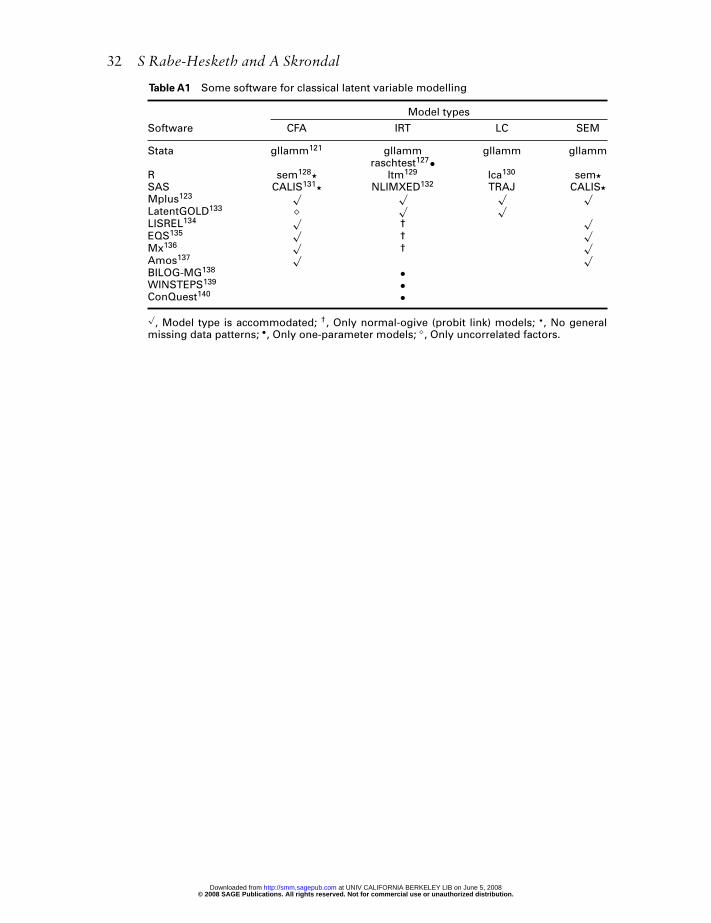
32 S Rabe-Hesketh and A Skrondal
Table A1 Some software for classical latent variable modelling
Model types
Software CFA IRT LC SEM
Stata gllamm121 gllamm gllamm gllammraschtest127•
R sem128� ltm129 lca130 sem�
SAS CALIS131� NLIMXED132 TRAJ CALIS�
Mplus123 √ √ √ √LatentGOLD133 √ √LISREL134 √
†√
EQS135 à
√Mx136 √
†√
Amos137 √ √BILOG-MG138 •WINSTEPS139 •ConQuest140 •√
, Model type is accommodated; †, Only normal-ogive (probit link) models; �, No generalmissing data patterns; •, Only one-parameter models; , Only uncorrelated factors.
© 2008 SAGE Publications. All rights reserved. Not for commercial use or unauthorized distribution. at UNIV CALIFORNIA BERKELEY LIB on June 5, 2008 http://smm.sagepub.comDownloaded from