topologically-constrained latent variable...

Topologically-Constrained Latent Variable Models

Raquel Urtasun [email protected]

UC Berkeley EECS & ICSI; CSAIL MIT

David J. Fleet [email protected]

University of Toronto

Andreas Geiger [email protected]

Karlsruhe Institute of Technology

Jovan Popovic [email protected]

CSAIL MIT

Trevor J. Darrell [email protected]

UC Berkeley EECS & ICSI; CSAIL MIT

Neil D. Lawrence [email protected]

University of Manchester

Abstract

In dimensionality reduction approaches, thedata are typically embedded in a Euclideanlatent space. However for some data sets thisis inappropriate. For example, in human mo-tion data we expect latent spaces that arecylindrical or a toroidal, that are poorly cap-tured with a Euclidean space. In this paper,we present a range of approaches for embed-ding data in a non-Euclidean latent space.Our focus is the Gaussian Process latent vari-able model. In the context of human motionmodeling this allows us to (a) learn modelswith interpretable latent directions enabling,for example, style/content separation, and(b) generalise beyond the data set enablingus to learn transitions between motion styleseven though such transitions are not presentin the data.

1. Introduction

Dimensionality reduction is a popular approach todealing with high dimensional data sets. It is of-ten the case that linear dimensionality reduction, suchas principal component analysis (PCA) does not ad-equately capture the structure of the data. For this

Appearing in Proceedings of the 25 th International Confer-ence on Machine Learning, Helsinki, Finland, 2008. Copy-right 2008 by the author(s)/owner(s).

reason there has been considerable interest in the ma-chine learning community in non-linear dimensionalityreduction. Approaches such as locally linear embed-ding (LLE), Isomap and maximum variance unfold-ing (MVU) (Roweis & Saul, 2000; Tenenbaum et al.,2000; Weinberger et al., 2004) all define a topologythrough interconnections between points in the dataspace. However, if a given data set is relatively sparseor particularly noisy, these interconnections can straybeyond the ‘true’ local neighbourhood and the result-ing embedding can be poor.

Probabilistic formulations of latent variable models donot usually include explicit constraints on the embed-ding and therefore the natural topology of the datamanifold is not always respected 1. Even with the cor-rect topology and dimension of the latent space, thelearning might get stuck in local minima if the initial-ization of the model is poor. Moreover, the maximumlikelihood solution may not be a good model, due e.g.,to the sparseness of the data. To get better models insuch cases, more constraints on the model are needed.

This paper shows how explicit topological constraintscan be imposed within the context of probabilistic la-tent variable models. We describe two approaches,both within the context of the Gaussian process la-tent variable model (GP-LVM) (Lawrence, 2005). The

1An exception is the back-constrained GP-LVM(Lawrence & Quinonero-Candela, 2006) where a con-strained maximum likelihood algorithm is used to enforcethese constraints.


first uses prior distributions on the latent space thatencourage a given topology. The second influencesthe latent space and optimisation through constrainedmaximum likelihood.

Our approach is motivated by the problem of model-ing human pose and motion for character animation.Human motion is an interesting domain because, whilethere is an increasing amount of motion capture dataavailable, the diversity of human motion means thatwe will necessarily have to incorporate a large amountof prior knowledge to learn probabilistic models thatcan accurately reconstruct a wide range of motions.Despite this, most existing methods for learning poseand motion models (Elgammal & Lee, 2004; Grochowet al., 2004; Urtasun et al., 2006) do not fully exploituseful prior information, and many are limited to mod-eling a single human activity (e.g., walking with a par-ticular style).

This paper describes how prior information can beused effectively to learn models with specific topologiesthat reflect the nature of human motion. Importantly,with this information we can also model multiple ac-tivities, including transitions between them (e.g. fromwalking to running), even when such transitions arenot present in the training data. As a consequence,we can now learn latent variable models with trainingmotions comprising multiple subjects with stylistic di-versity, as well as multiple activities, such as runningand walking. We demonstrate the effectiveness of ourapproach in a character animation application, wherethe user specifies a set of constraints (e.g., foot loca-tions), and the remaining kinematic degrees of freedomare infered.

2. Gaussian Process Latent VariableModels (GP-LVM)

We begin with a brief review of the GP-LVM(Lawrence, 2005). The GP-LVM represents a high-dimensional data set, Y, through a low dimensionallatent space, X, and a Gaussian process mappingfrom the latent space to the data space. Let Y =[y1, ...,yN ]T be a matrix in which each row is a singletraining datum, yi ∈ ℜD. Let X = [x1, ...,xN ]T de-note the matrix whose rows represent the correspond-ing positions in latent space, xi ∈ ℜd. Given a covari-ance function for the Gaussian process, kY (x,x′), thelikelihood of the data given the latent positions is,

p(Y |X, β) =1

Z1exp

(

−1

2tr

(

K−1Y YYT

)

)

, (1)

where Z1 is a normalization factor, KY is known asthe kernel matrix, and β denotes the kernel hyperpa-rameters. The elements of the kernel matrix are de-

fined by the covariance function, (KY )i,j = kY (xi,xj).A common choice is the radial basis function (RBF),

kY (x,x′) = β1 exp(−β2

2 ||x− x′||2) +δx,x′

β3

, where the

kernel hyperparameters β = {β1, β2, β3} determine theoutput variance, the RBF support width, and the vari-ance of the additive noise. Learning in the GP-LVMconsists of maximizing (1) with respect to the latentpositions, X, and the hyperparameters, β.

When one has time-series data, Y represents a se-quence of observations, and it is natural to aug-ment the GP-LVM with an explicit dynamical model.For example, the Gaussian Process Dynamical Model(GPDM) models the sequence as a latent stochasticprocess with a Gaussian process prior (Wang et al.,2008) , i.e.,

p(X | α) =p(x1)

Z2exp

(

−1

2tr

(

K−1X XoutX

Tout

)

)

(2)

where Z2 is a normalization factor, Xout =[x2, ...,xN ]T , KX ∈ ℜ(N−1)×(N−1) is the kernel matrixconstructed from Xin = [x1, ...,xN−1], x1 is given anisotropic Gaussian prior and α are the kernel hyper-parameters for KX ; below we use an RBF kernel forKX . Like the GP-LVM the GPDM provides a gen-erative model for the data, but additionally it pro-vides one for the dynamics. One can therefore predictfuture observation sequences given past observations,and simulate new sequences.

3. Top Down Imposition of Topology

The smooth mapping in the GP-LVM ensures thatdistant points in data space remain distant in la-tent space. However, as discussed in (Lawrence &Quinonero-Candela, 2006), the mapping in the oppo-site direction is not required to be smooth. Whilethe GPDM may mitigate this effect, it often producesmodels that are neither smooth nor generalize well(Urtasun et al., 2006; Wang et al., 2008).

To help ensure smoother, well-behaved models,(Lawrence & Quinonero-Candela, 2006) suggested theuse of back-constraints, where each point in the latentspace is a smooth function of its corresponding pointin data space, xij = gj (yi;aj), where {aj}1≤j≤d isthe set of parameters of the mappings. One possiblemapping is a kernel-based regression model, where re-gression on a kernel induced feature space provides themapping,

xij =N

∑

m=1

ajmk(yi,ym) . (3)

This approach is known as the back-constrained GP-LVM. When learning the back-constrained GP-LVM,


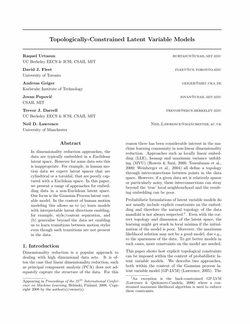
(a) (b) (c) (d)Figure 1. When training data contain large stylistic variations and multiple motions, the generic GPDM (a) and theback-constrained GPDM (b) do not produce useful models. Simulations of both models here do not look realistic. (c,d)Hybrid model learned using local linearities for smoothness (i.e., style) and backconstraints for topologies (i.e., content).The training data is composed of 9 walks and 10 runs performed by different subjects and speeds. (c) Likelihood for thereconstruction of the latent points (d) 3D view of the latent trajectories for the training data in blue, and the automaticallygenerated motions of Figs. 3 and 4 in green and red respectively.

one needs to determine the hyperparameters of the ker-nel matrices (for the back-constraints and the covari-ance of the GP), as well as the mapping weights, {aj}.(Lawrence & Quinonero-Candela, 2006) fixed the hy-perparameters of the back-constraint’s kernel matrix,optimizing over the remaining parameters.

Nevertheless, when learning human motion data withlarge stylistic variations or different motions, nei-ther GPDM nor back-constrained GP-LVM producesmooth models that generalize well. Fig. 1 depictsthree 3–D models learned from 9 walks and 10 runs.The GPDM (Fig. 1(a)) and the back-constraintedGPDM2 (Fig. 1 (b)) do not generalize well to new runsand walks, nor do they produce realistic animations.

In this paper we show that with a well designedset of back-constraints good models can be learned(Fig. 1(c)). We also consider an alternative approachto the hard constraints on the latent space arisingfrom gj (yi;aj). We introduce topological constraintsthrough a prior distribution in the latent space, basedon a neighborhood structure learned through a gener-alized local linear embedding (LLE) (Roweis & Saul,2000). We then show how to incorporate domain-specific prior knowledge, which allows us to developmotion models with specific topologies that incorpo-rate different activities within a single latent space andtransitions between them.

3.1. Locally Linear GP-LVM

The locally linear embedding (LLE) (Roweis & Saul,2000) preserves topological constraints by finding arepresentation based on reconstruction in a low dimen-sional space with an optimized set of local weightings.Here we show how the LLE objective can be combinedwith the GP-LVM, yielding a locally linear GP-LVM

(LL-GPLVM).

2We use an RBF kernel for the inverse mapping in (3).

The locally linear embedding assumes that each datapoint and its neighbors lie on, or close to, a locallylinear patch on the data manifold. The local geome-try of these patches can then be characterized by lin-ear coefficients that reconstruct each data point fromits neighbors. This is done in a three step proce-dure: (1) the K nearest neighbors, {yj}j∈ηi

, of eachpoint, yi, are computed using Euclidean distance inthe input space, dij = ||yi − yj ||

2; (2) the weightsw = {wij} that best reconstruct each data pointfrom its neighbors are obtained by minimizing Φ(w) =∑Ni=1 ||yi−

∑

j∈ηiwijyj ||

2; and (3) the latent positionsxi best reconstructed by the weights wij are computed

by minimizing Φ(X) =∑Ni=1 ||xi −

∑

j∈ηiwijxj ||

2.

In the LLE, the weight matrix w is sparse (only a smallnumber of neighbors is used), and the two minimiza-tions can be computed in closed form. In particular,computing the weights can be done by solving, ∀j ∈ ηi,the following system,

∑

k

Csimkj wsimij = 1 , (4)

where Csimkj = (yi − yk)T (yi − yj) if j, k ∈ ηi, and 0

otherwise. Once the weights are computed, they arerescaled so that

∑

j wij = 1.

The LLE energy function can be interpreted, for agiven set of weights w, as a prior that forces eachlatent point to be locally reconstructed by its neigh-bors,i.e., p(X|w) = 1

Zexp

{

− 1σ2 Φ(X)

}

, where Z isa normalization constant, and σ2 represents a globalscaling of the prior. Note that strictly speaking this isnot a proper prior as it is conditioned on the weightswhich depend on the training data. Following (Roweis& Saul, 2000), we first compute the neighbors basedon the Euclidean distance. For each training point yi,we then compute the weights solving Eq. (4).

Learning the LL-GPLVM is then equivalent to mini-


mizing the negative log posterior of the model, 3 i.e.,

LS = log p(Y|X, β) p(β) p(X|w)

=D

2ln |KY | +

1

2tr

(

K−1Y YYT

)

+∑

i

lnβi

+1

σ2

d∑

k=1

N∑

i=1

‖xki −N

∑

j=1

wkijxkj ‖

2 + C , (5)

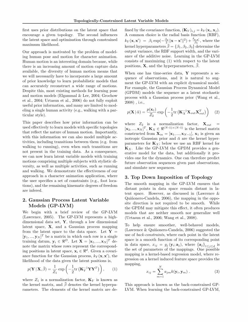
where C is a constant, and xki is the k-th componentof xi. Note that we have extended the LLE to havea different prior for each dimension. This will be use-ful below as we incorporate different sources of priorknowledge. Fig. 2 (a) shows a model of 2 walks and 2runs learned with the locally linear GPDM. Note howsmooth the latent trajectories are.

We now have general tools to influence the structureof the models. In what follows we generalize the top-down imposition of topology strategies (i.e. back-constraints and locally linear GP-LVM) to incorporatedomain specific prior knowledge.

4. Reflecting Knowledge in LatentSpace Structure

A problem for modeling human motion data is thesparsity of the data relative to the diversity of natu-rally plausible motions. For example, while we mighthave a data set comprising different motions, such asruns, walks etc., the data may not contain transitionsbetween motions. In practice however, we know thatthese motions will be approximately cyclic and thattransitions can only physically occur at specific pointsin the cycle. How can we encourage a model to re-spect such topological constraints which arise fromprior knowledge?

We consider two alternatives to solve this problem.First, we show how one can adjust the distance metricused in the locally linear embedding to better reflectdifferent types of prior knowledge. We then show howone can define similarity measures for use with theback-constrained GP-LVM. Both these approaches en-courage the latent space to construct a representationthat reflects our prior knowledge. They are comple-mentary and can be combined to learn better models.

3When learning a locally linear GPDM, the dynamicsand the locally linear prior are combined as a product of po-tentials. The objective function becomes LS + d

2ln |KX |+

1

2tr

`

K−1

XXoutX

T

out

´

+P

iln αi, with LS defined as in (5).

(a) (d)

(b) (e)

(c) (f)Figure 2. First two dimensions of 3–D models learnedusing (a) LL-GPDM (b) LL-GPDM with topology (c)LL-GPDM with topology and transitions. (d) Back-constrained GPDM with an RBF mapping. (e) GPDMwith topology through backconstraints. (f) GPDM withbackconstraints for the topology and transitions. For themodels using topology, the cyclic structure is imposed inthe last 2 dimensions. The two types of transition points(left and right leg contact points) are shown in red andgreen, and are used as prior knowledge in (c,f).

4.1. Prior Knowledge through Local

Linearities

We now turn to consider how one might incorporateprior knowledge in the LL-GPLVM framework. This isaccomplished by replacing the local Euclidean distancemeasures used in Section 3.1 with other similarity mea-sures. That is, we can modify the covariance used tocompute the weights in Eq. (4) to reflect our priorknowledge in the latent space. We consider two exam-ples: the first involves transitions between activities;with the second we show how topological constraintscan be placed on the form of the latent space.

Covariance for Transitions Modeling transitionsbetween motions is important in character animation.Transitions can be infered automatically based on sim-ilarity between poses (Kovar et al., 2002) or at pointsof non-linearity of the dynamics (Bissacco, 2005), andthey can be used for learning. For example, for mo-tions as walking or running, two types of transitionscan be identified: left and right foot ground contacts.


To model such transitions, we define an index on theframes of the motion sequence, {ti}

Ni=1. We then define

subsets of this set, {ti}Mi=1, which represents frames

where transitions are possible. To capture transitionsin the latent model we define the elements for the co-variance matrix as follows,

Ctranskj = 1 −[

δkj exp(−ζ(tk − tj)2)

]

(6)

with ζ a constant, and δij = 1 if ti and tj are in thesame set {tk}

Mk=1, and otherwise δij = 0. This covari-

ance encourages the latent points at which transitionsare physically possible to be close together.

Covariance for Topologies We now consider co-variances that encourage the latent space to have aparticular topology. Specifically we are interested insuitable topologies for walking and running data. Be-cause the data are approximately periodic, it seemsappropriate to have a non-Cartesian topology. To thisend one can extract the phase of the motion4, φ, anduse it with a covariance to encourage the latent pointsto exhibit a periodic topological structure within aCartesian space. As an example we consider a cylindri-cal topology within a 3–D latent space by constrainingtwo of the latent dimensions with the phase. In partic-ular, to represent the cyclic motion we construct a dis-tance function on the unit circle, where a latent pointcorresponding to phase φ is represented with coordi-nates (cos(φ), sin(φ)). To force a cylindrical topologyon the latent space, we specify different covariances foreach latent dimension

Ccosk,j = (cos(φi) − cos(φk)) (cos(φi) − cos(φj)) (7)

Csink,j = (sin(φi) − sin(φk)) (sin(φi) − sin(φj)) , (8)

with k, j ∈ ηi. The covariance for the remaining di-mension is constructed as usual, based on Euclideandistance in the data space. Fig. 2 (b) shows a GPDMconstrained in this way, and in Fig. 2 (c) the covari-ance is augmented with transitions.

Note that the use of different distance measures foreach dimension of the latent space implies that theneighborhood and the weights in the locally linearprior will also be different for each dimension. Here,three different locally linear embeddings form the priordistribution.

4.2. Prior Knowledge with Back Constraints

As explained above, we can also design back-constraints to influence the topology and learn useful

4The phase can be easily extracted from the data byFourier analysis or by detecting key postures and interpo-lating the phases between them. Another idea, not furtherexplored here, would be to optimize the GP-LVM with re-spect to the phase.

transitions. This can be done by replacing the ker-nel of Eq. (3). Many kernels have interpretations assimilarity measures. In particular, any similarity mea-sure that leads to a positive semi-definite matrix canbe interpreted as a kernel. Here, just as we definecovariance matrices above, we extend the original for-mulation of back constraints by constructing similaritymeasures (i.e., kernels) to reflect prior knowledge.

Similarity for Transitions To capture transitionsbetween two motions, we wish to design a kernel thatexpresses strong similarity between points in the re-spective motions where transitions may occur. We canencourage transition points of different sequences tobe proximal with the following kernel matrix for theback-constraint mapping:

ktrans(ti, tj) =∑

m

∑

l

δmlk(ti, tm)k(tj , tl) (9)

where k(ti, tl) is an RBF centered at tl, and δml = 1if tm and tl are in the same set. The influence of theback-constraints is controlled by the support width ofthe RBF kernel.

Topologically Constrained Latent Spaces Wenow consider kernels that force the latent space to havea particular topology. To force a cylindrical topologyon the latent space, we can introduce similarity mea-sures based on the phase, specifying different similaritymeasures for each latent dimension. As before we con-struct a distance function in the unit circle, that takesinto account the phase. A periodic mapping can beconstructed from a kernel matrix as follows,

xn,1 =

N∑

m=1

acosm k(cos(φn), cos(φm)) + acos0 δn,m,

xn,2 =

N∑

m=1

asinm k(sin(φn), sin(φm)) + asin0 δn,m,

where k is an RBF kernel function, and xn,i is the ith

coordinate of the nth latent point. These two map-pings project onto two dimensions of the latent space,forcing them to have a periodic structure (which comesabout through the sinusoidal dependence of the kernelon phase). Fig. 2 (e) shows a model learned usingGPDM with the last two dimensions constrained inthis way (the third dimension is out of plane). Thefirst dimension is constrained by an RBF mapping onthe input space. Each dimension’s kernel matrix canthen be augmented by adding the transition similarityof Eq.(9), resulting in the model shown in Fig. 2 (f).

4.3. Model Combination

One advantage of our framework is that covariance ma-trices can be combined in a principled manner to form


new covariance matrices. Covariances can be multi-plied (on an element by element basis) or added to-gether. Similarly, similarities can be combined. Mul-tiplication has, loosely speaking, an ‘AND gate effect’,i.e. both similarity measures must agree that an ob-ject is similar for their product to express similarity.Adding them produces more of an ‘OR gate effect’, i.e.if either representation expresses similarity the result-ing measure will also express similarity.

The two sections above have shown how to incorpo-rate prior knowledge in the GP-LVM by means of 1)local linearities and 2) back-constraints. In general,the latter should be used when the manifold has awell-defined topology, since it has more influence onthe learning. When the topology is not so well defined(e.g., due to noise) one should use local linearities.Both techniques are complementary and can be com-bined straightforwardly by including priors over somedimensions, and constraining the others through back-constraint mappings. Fig. 1 shows a model learnedwith LL-GPDM for smoothness and back-constraintsfor topology.

4.4. Multiple Activities and Transitions

Once we know how to ensure that transition points areclose together and that the latent structure has thedesired topology, we still need to address two issues.How do we learn models that have very different dy-namics? How can we simulate dynamical models thatlie somewhere between the different training motions?Our goal in this section is to show how latent mod-els for different motions can be learned independently,but in a shared latent space that facilitates transitionsbetween activities with different dynamics.

Let Y = [YT1 , ..., Y

TM ]T denote training data for M

different activities. Each Ym comprises several differ-ent motions. Let X = [XT

1 , ..., XTM ]T denote the corre-

sponding latent positions. When dealing with multipleactivities, a single dynamical model cannot cope withthe complexity of the different dynamics. Instead, weconsider a model where the dynamics of each activityare modeled independently5. This has the advantagethat a different kernel can be used for each activity.

To enable interpolation between motions with differentdynamics, we combined these independent dynamicalmodels in the form of a mixture model. This allows usto produce motions that gracefully transition betweendifferent styles and motion types (Figs. 3 and 4).

5Another interpretation is that we have a block diagonalkernel matrix for the GP that governs the dynamics.

5. Results

We demonstrate the effectiveness of our approach withtwo applications. First we show how models of multi-ple activities can be learned, and realistic animationscan be produced by drawing samples from the model.We then show an interactive character animation ap-plication, where the user specifies a set of sparse con-straints and the remaining kinematic degrees of free-dom are infered.

5.1. Learning multiple activities

We first considered a small training set comprised of4 gait cycles (2 walks and 2 runs) performed by onesubject at different speeds. Fig. 2 shows the latentspaces learned under different prior constraints. Allthe models are learned using two independent dynam-ical models, one for walking and one for running. Notehow the phases are aligned when imposing a cylindricaltopology, and how the LL-GPDM is smooth. Noticethe difference between the LL-GPDM (Fig. 2 (c)) andthe backconstrained GPDM (Fig. 2 (f)) when transi-tion constraints are included. Neverthess, both mod-els ensure that the transition points (shown in red andgreen) are proximal.

Fig. 1 (c) shows a hybrid model learned using LL-GPDM for smoothness, and back-constraints for topol-ogy. The larger training set comprises approximatelyone gait cycle from each of 9 walking and 10 runningmotions performed by different subjects at differentspeeds (3 km/h for walking, 6–12 km/h for running).Colors in Fig. 1 (a) represent the variance of the GPas a function of latent position. Only points close tothe surface of the cylinder produce poses with highcertainty.

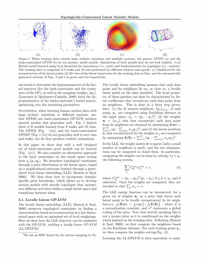
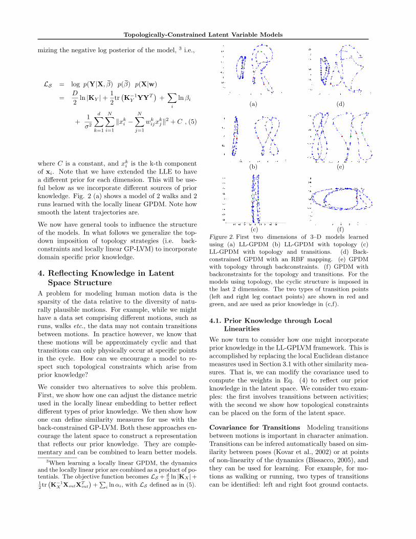
We now illustrate the model’s ability to simulate dif-ferent motions and transitions. Given an initial la-tent position x0, we generate new motions by sam-pling the mixture model, and using mean predictionfor the reconstruction. Choosing different initial con-ditions results in very different simulations (Fig. 1 (d)).The training data are shown in blue. For the firstsimulation (depicted in green), the model is initial-ized to a running pose with a latent position not farfrom walking data. The system transitions to walkingquite naturally. The resulting animation is depicted inFig. 3. For the second example (in red), we initializethe simulation to a latent position far from walkingdata. The system evolves to different running stylesand speeds (Fig. 4). Note how the dynamics, and thestrike length, change considerably during simulation.


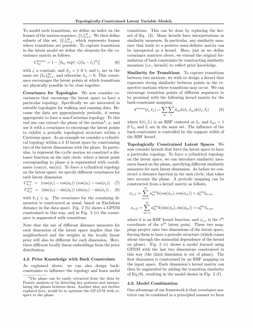
Figure 3. Transition from running to walking: The system transitions from running to walking in a smooth andrealistic way. The transition is encouraged by incorporating prior knowledge in the model. The latent trajectories areshown in green in Fig. 1 (d).

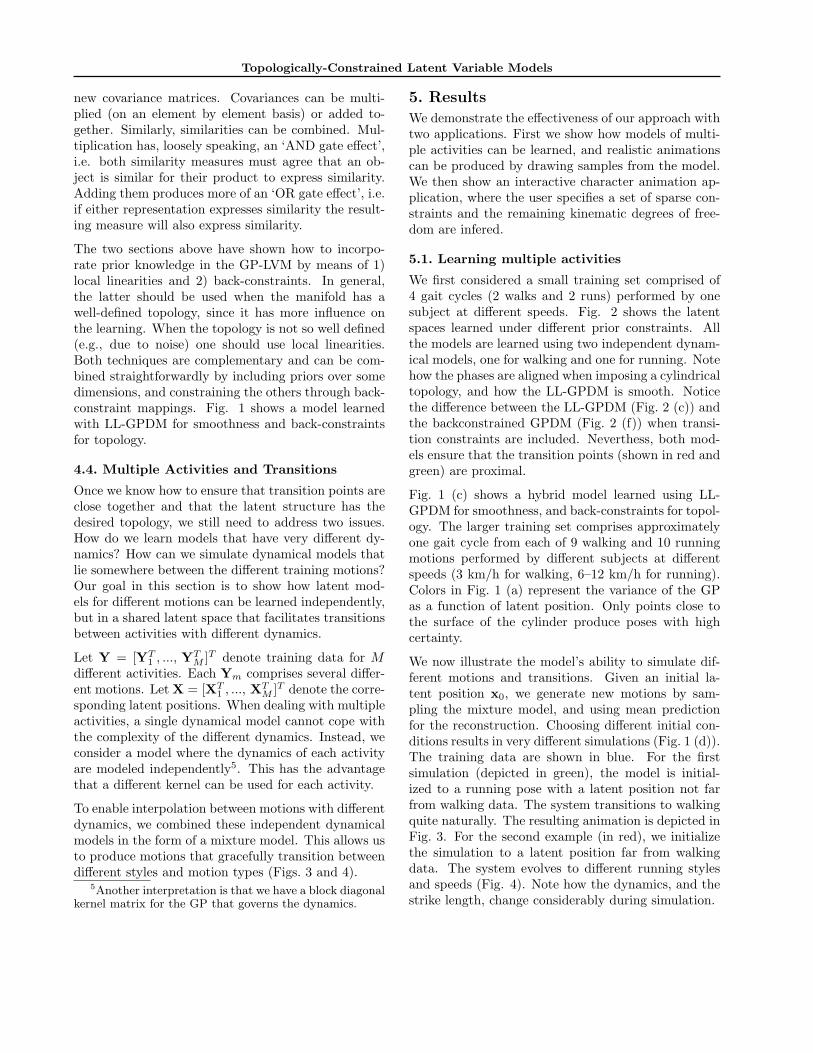
Figure 4. Different running styles and speeds: The system is able to simulate a motion with considerably changesin speed and style. The latent trajectories are shown in red in Fig. 1 (d).

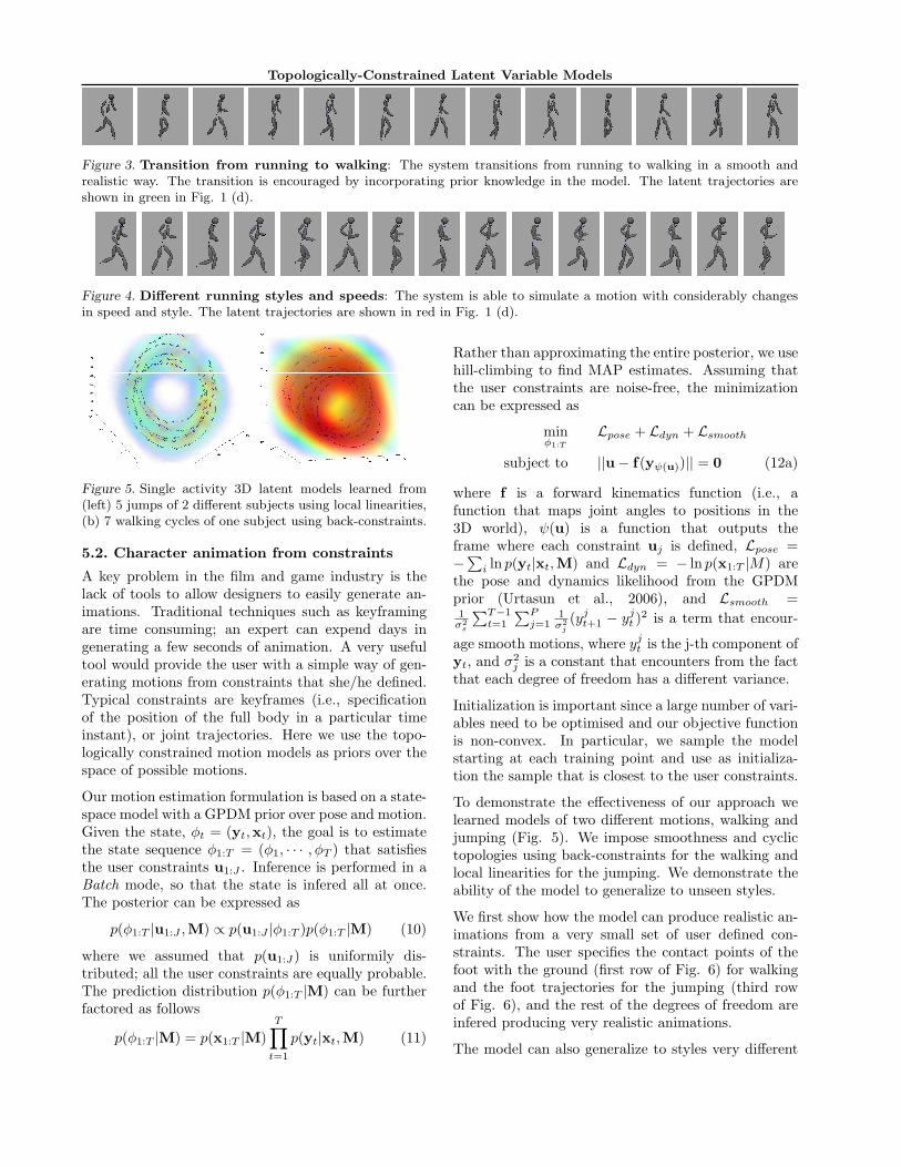
Figure 5. Single activity 3D latent models learned from(left) 5 jumps of 2 different subjects using local linearities,(b) 7 walking cycles of one subject using back-constraints.

5.2. Character animation from constraints

A key problem in the film and game industry is thelack of tools to allow designers to easily generate an-imations. Traditional techniques such as keyframingare time consuming; an expert can expend days ingenerating a few seconds of animation. A very usefultool would provide the user with a simple way of gen-erating motions from constraints that she/he defined.Typical constraints are keyframes (i.e., specificationof the position of the full body in a particular timeinstant), or joint trajectories. Here we use the topo-logically constrained motion models as priors over thespace of possible motions.

Our motion estimation formulation is based on a state-space model with a GPDM prior over pose and motion.Given the state, φt = (yt,xt), the goal is to estimatethe state sequence φ1:T = (φ1, · · · , φT ) that satisfiesthe user constraints u1:J . Inference is performed in aBatch mode, so that the state is infered all at once.The posterior can be expressed as

p(φ1:T |u1:J ,M) ∝ p(u1:J |φ1:T )p(φ1:T |M) (10)

where we assumed that p(u1:J ) is uniformily dis-tributed; all the user constraints are equally probable.The prediction distribution p(φ1:T |M) can be furtherfactored as follows

p(φ1:T |M) = p(x1:T |M)T

∏

t=1

p(yt|xt,M) (11)

Rather than approximating the entire posterior, we usehill-climbing to find MAP estimates. Assuming thatthe user constraints are noise-free, the minimizationcan be expressed as

minφ1:T

Lpose + Ldyn + Lsmooth

subject to ||u − f(yψ(u))|| = 0 (12a)

where f is a forward kinematics function (i.e., afunction that maps joint angles to positions in the3D world), ψ(u) is a function that outputs theframe where each constraint uj is defined, Lpose =−

∑

i ln p(yt|xt,M) and Ldyn = − ln p(x1:T |M) arethe pose and dynamics likelihood from the GPDMprior (Urtasun et al., 2006), and Lsmooth =1σ2

s

∑T−1t=1

∑Pj=1

1σ2

j

(yjt+1 − yjt )

2 is a term that encour-

age smooth motions, where yjt is the j-th component ofyt, and σ2

j is a constant that encounters from the factthat each degree of freedom has a different variance.

Initialization is important since a large number of vari-ables need to be optimised and our objective functionis non-convex. In particular, we sample the modelstarting at each training point and use as initializa-tion the sample that is closest to the user constraints.

To demonstrate the effectiveness of our approach welearned models of two different motions, walking andjumping (Fig. 5). We impose smoothness and cyclictopologies using back-constraints for the walking andlocal linearities for the jumping. We demonstrate theability of the model to generalize to unseen styles.

We first show how the model can produce realistic an-imations from a very small set of user defined con-straints. The user specifies the contact points of thefoot with the ground (first row of Fig. 6) for walkingand the foot trajectories for the jumping (third rowof Fig. 6), and the rest of the degrees of freedom areinfered producing very realistic animations.

The model can also generalize to styles very different


510

15

−35−30

−25−20

−15−10

−50

510

15

0

5

10

15

20

25

x

z

y

510

15

−35−30

−25−20

−15−10

−50

510

15

0

5

10

15

20

25

x

z

y

510

15

−35−30

−25−20

−15−10

−50

510

15

0

5

10

15

20

25

x

z

y

510

15

−35−30

−25−20

−15−10

−50

510

15

0

5

10

15

20

25

x

z

y

510

15

−35−30

−25−20

−15−10

−50

510

15

0

5

10

15

20

25

x

z

y

510

15

−40

−30

−20

−10

0

10

0

5

10

15

20

25

x

z

y

510

15

−40

−30

−20

−10

0

10

0

5

10

15

20

25

x

z

y

510

15

−40

−30

−20

−10

0

10

0

5

10

15

20

25

x

z

y

510

15

−40

−30

−20

−10

0

10

0

5

10

15

20

25

x

z

y

510

15

−40

−30

−20

−10

0

10

0

5

10

15

20

25

x

z

y

−30 −25 −20 −15 −10 −50

5

10

15

20

25

30

35

z

y

−30 −25 −20 −15 −10 −50

5

10

15

20

25

30

35

z

y

−30 −25 −20 −15 −10 −50

5

10

15

20

25

30

35

z

y

−30 −25 −20 −15 −10 −50

5

10

15

20

25

30

35

z

y

−30 −25 −20 −15 −10 −50

5

10

15

20

25

30

35

z

y

−30 −25 −20 −15 −10 −50

5

10

15

20

25

30

35

z

y

−30 −25 −20 −15 −10 −50

5

10

15

20

25

30

35

z

y

−30 −25 −20 −15 −10 −50

5

10

15

20

25

30

35

z

y

−35 −30 −25 −20 −15 −10 −5 0

0

5

10

15

20

25

30

z

y

−35 −30 −25 −20 −15 −10 −5 0

0

5

10

15

20

25

30

z

y

−35 −30 −25 −20 −15 −10 −5 0

0

5

10

15

20

25

30

z

y

−35 −30 −25 −20 −15 −10 −5 0

0

5

10

15

20

25

30

z

y

−35 −30 −25 −20 −15 −10 −5 0

0

5

10

15

20

25

30

zy

−35 −30 −25 −20 −15 −10 −5 0

0

5

10

15

20

25

30

z

y

−35 −30 −25 −20 −15 −10 −5 0

0

5

10

15

20

25

30

z

y

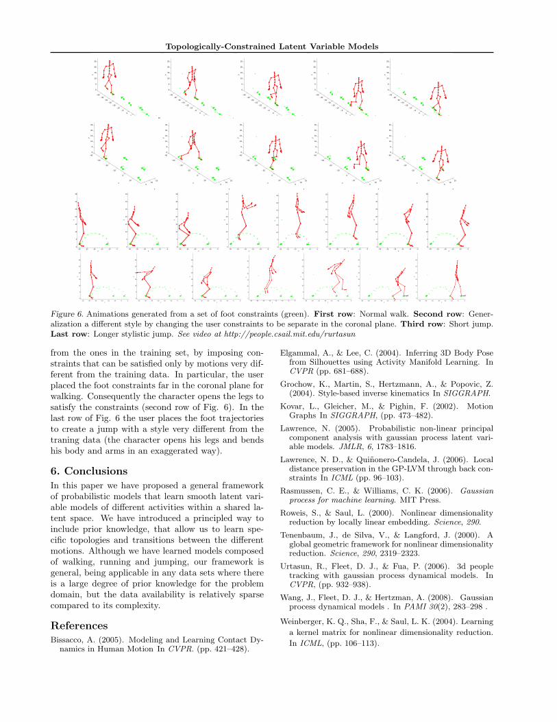
Figure 6. Animations generated from a set of foot constraints (green). First row: Normal walk. Second row: Gener-alization a different style by changing the user constraints to be separate in the coronal plane. Third row: Short jump.Last row: Longer stylistic jump. See video at http://people.csail.mit.edu/rurtasun

from the ones in the training set, by imposing con-straints that can be satisfied only by motions very dif-ferent from the training data. In particular, the userplaced the foot constraints far in the coronal plane forwalking. Consequently the character opens the legs tosatisfy the constraints (second row of Fig. 6). In thelast row of Fig. 6 the user places the foot trajectoriesto create a jump with a style very different from thetraning data (the character opens his legs and bendshis body and arms in an exaggerated way).

6. Conclusions

In this paper we have proposed a general frameworkof probabilistic models that learn smooth latent vari-able models of different activities within a shared la-tent space. We have introduced a principled way toinclude prior knowledge, that allow us to learn spe-cific topologies and transitions between the differentmotions. Although we have learned models composedof walking, running and jumping, our framework isgeneral, being applicable in any data sets where thereis a large degree of prior knowledge for the problemdomain, but the data availability is relatively sparsecompared to its complexity.

ReferencesBissacco, A. (2005). Modeling and Learning Contact Dy-

namics in Human Motion In CVPR. (pp. 421–428).

Elgammal, A., & Lee, C. (2004). Inferring 3D Body Posefrom Silhouettes using Activity Manifold Learning. InCVPR (pp. 681–688).

Grochow, K., Martin, S., Hertzmann, A., & Popovic, Z.(2004). Style-based inverse kinematics In SIGGRAPH.

Kovar, L., Gleicher, M., & Pighin, F. (2002). MotionGraphs In SIGGRAPH, (pp. 473–482).

Lawrence, N. (2005). Probabilistic non-linear principalcomponent analysis with gaussian process latent vari-able models. JMLR, 6, 1783–1816.

Lawrence, N. D., & Quinonero-Candela, J. (2006). Localdistance preservation in the GP-LVM through back con-straints In ICML (pp. 96–103).

Rasmussen, C. E., & Williams, C. K. (2006). Gaussianprocess for machine learning. MIT Press.

Roweis, S., & Saul, L. (2000). Nonlinear dimensionalityreduction by locally linear embedding. Science, 290.

Tenenbaum, J., de Silva, V., & Langford, J. (2000). Aglobal geometric framework for nonlinear dimensionalityreduction. Science, 290, 2319–2323.

Urtasun, R., Fleet, D. J., & Fua, P. (2006). 3d peopletracking with gaussian process dynamical models. InCVPR, (pp. 932–938).

Wang, J., Fleet, D. J., & Hertzman, A. (2008). Gaussianprocess dynamical models . In PAMI 30(2), 283–298 .

Weinberger, K. Q., Sha, F., & Saul, L. K. (2004). Learning

a kernel matrix for nonlinear dimensionality reduction.

In ICML, (pp. 106–113).

topologically-constrained latent variable...

Documents